Electron transfer dynamics using projected modes

Abstract

For electron-phonon Hamiltonians with the couplings linear in the phonon operators we construct a class of unitary transformations that separate the normal modes into two groups. The modes in the first group interact with the electronic degrees of freedom directly. The modes in the second group interact directly only with the modes in the first group but not with the electronic system. We show that for the $n$-level electronic system the minimum number of modes in the first group is $n_{s}=(n^{2}+n-2)/2$. The separation of the normal modes into two groups allows one to develop new approximation schemes. We apply one of such schemes to study exitonic relaxation in a model semiconducting molecular heterojuction.

I Introduction

One of the central assumptions in formulating the relaxation dynamics of a quantum system embedded in a condensed media is the partitioning between degrees of freedom treated explicitly and implicitly. Often, we are guided by our “physical intuition” in separating the system (explicit degrees of freedom) from the bath (implicit degrees of freedom). This intuitive approach breaks-down severely when the coupling between system and bath degrees of freedom become too strong. This situation is exasperated when one attempts to treat some of the degrees of freedom using quantum mechanics and the remaining degrees of freedom using classical mechanics. What is clearly lacking is a unambiguous approach for formally partitioning a system with both discrete and continuous degrees of freedom into interacting sub-spaces such that the motions that are most strongly coupled are given explicit treatment while the remainder serve as auxiliary degrees of freedom (quantum or classical), as a thermal bath, or are ignored completely. Clearly, such a partitioning is dependent upon the specific system at hand. However, the prescription for making the partitioning should be universal and depend only upon the form of the original Hamiltonian.

In many respects, we anticipate the presence of “special” degrees of freedom. One of the central tenants of modern chemical physics is that of the reaction coordinate, espectially in the Marcus-Hush model of charge-transfer between donor and acceptor species. The reaction coordinate that parameterizes the free-energy parabolas in this classic model are not explicitly defined in terms of actual nuclear motions. The driving force, electronic coupling, and reorganization energy terms appearing in the Marcus-Hush expression for the electron-transfer rate are all experimentally derived quantities. Nuclear motion enters into the description when we make the connection between the polarization field and the reorganization and relaxation of the donor and acceptor molecules and their surroundings.

In this paper we present a procedure for deducing the reaction coordinate for a multidimensional electron transfer process. By using a series of canonical transformations we can uniquely decompose the fully-coupled problem into a subset of strongly correlated vibronic motions that have clear dynamical and structural meaning and carry all of the electron/phonon couplings. This subspace is coupled to the remaining vibrational degrees of freedom which in turn are completely decoupled from the electron transfer dynamics, but serve as a dissipative subsystem.

II Projected modes

A wide class of the electron-phonon systems is described by the following Hamiltonian

$$H=\sum_{a=1}^{n}\epsilon_{a}|a\rangle\langle a|+\sum_{a=b=1}^{n}\sum_{i=1}^{N}g_{abi}x_{i}|a\rangle\langle b|+\sum_{i=1}^{N}\frac{p_{i}^{2}}{2}+\sum_{i=1}^{N}\frac{\omega_{i}^{2}x_{i}^{2}}{2}.$$ (1)

Here $|a\rangle$’s denote electronic states with energies $\epsilon_{a}$, $x_{i}$ and $p_{i}$ are coordinate and momentum operators for the normal mode $i$ with frequency $\omega_{i}$, and $g_{abi}$ are the coupling parameters of the electron-phonon interaction. $N$ is the number of normal modes and $n$ is the number of electronic states. We seek to rewrite $H$ in terms of the new coordinate $X_{i}$ and momentum $P_{i}$ operators so that it has the following form

$$H=\sum_{a=1}^{n}\epsilon_{a}|a\rangle\langle a|+\sum_{a=b=1}^{n}\sum_{i=1}^{n_{s}}g^{\prime}_{abi}X_{i}|a\rangle\langle b|+\sum_{i=1}^{n_{s}}\sum_{j=n_{s}+1}^{N}\gamma^{\prime}_{ij}X_{i}X_{j}+\sum_{i=1}^{N}\frac{{P}_{i}^{2}}{2}+\sum_{i=1}^{N}\frac{{\omega^{\prime}}_{i}^{2}{X}_{i}^{2}}{2}.$$ (2)

where $n_{s}=\frac{n(n+1)}{2}$ and $\omega^{\prime}_{i}$ are the new oscillator frequencies. In the new Hamiltonian only $n_{s}$ modes are directly coupled to the electronic degrees of freedom with $g^{\prime}_{abi}$ being the new coupling parameters. We will refer to these modes as the system modes Gindensperger et al. (2006a, b). These $n_{s}$ modes are also coupled to the $N-n_{s}$ remaining normal modes (that are not directly coupled to the electronic degrees of freedom). We will call these $N-n_{s}$ modes the bath modes. Coefficients $\gamma^{\prime}_{ij}$ give the couplings between the system modes and the bath modes. The transition form Eq. (1) to Eq. (2) can be achieved by a suitable linear transformation of the coordinate and momentum operators.

Consider the following linear transformations

$$X_{i} = \sum_{j}M_{ij}x_{j},$$ (3)

$$P_{i} = \sum_{j}(\widetilde{M}^{-1})_{ij}p_{j}.$$ (4)

Here $M_{ij}$ are the elements of an arbitrary real matrix ${\bf M}$. We will assume that ${\bf M}$ has an inverse, ${\bf M}^{-1}$. ${\bf\widetilde{M}^{-1}}$ denotes the transpose of ${\bf M}^{-1}$. It can be shown that transformations (3) and (4) are canonical, i. e., $X_{i}$ and $P_{i}$ satisfy the usual commutation relations for coordinates and momenta. Since matrix ${\bf M}$ is real the new operators $X_{i}$ and $P_{i}$ are Hermitian. The inverse transformations are given by

$$x_{i} = \sum_{j}M^{-1}_{ij}X_{j},$$ (5)

$$p_{i} = \sum_{j}\widetilde{{M}}_{ij}P_{j}.$$ (6)

In Appendix A we show that transformations (3) and (4) can always be viewed as unitary transformations of operators $x_{i}$ and $p_{i}$.

Our goal of going to the new coordinates can be achieved with orthogonal matrices ${\bf M}$. Therefore, in this section we will assume that ${\bf M}$ is orthogonal, i. e., $\widetilde{\bf M}={\bf M}^{-1}$. We will discuss the possible uses of the non-orthogonal matrices below.

In order to obtain the explicit form of ${\bf M}$ we substitute expressions (5) and (6) for $x_{i}$ and $p_{i}$ into Eq. (1). This gives

$$H=\sum_{a=1}^{n}\epsilon_{a}|a\rangle\langle a|+\sum_{a=b=1}^{n}\sum_{i=1}^{N}\sum_{j=1}^{N}g_{abi}M^{-1}_{ij}X_{j}|a\rangle\langle b|+\sum_{i=1}^{N}\frac{P_{i}^{2}}{2}+\sum_{i=j=1}^{N}\frac{w_{ij}X_{i}X_{j}}{2}.$$ (7)

Here

$$w_{ij}=\sum_{k}M_{ik}\omega^{2}_{k}M^{-1}_{kj}.$$ (8)

Note that the momentum operators remain uncoupled for any orthogonal ${\bf M}$ in Eq. (6) because the matrix associated with the quadratic form $\sum_{i}p_{i}^{2}$ is the unit matrix and is invariant under the orthogonal transformations.

Hamiltonian (7) will have the form (2) if the following requirements are satisfied. First, the summation over $j$ in the second term has to extend only from $1$ to $n_{s}$. Second, the mode-mode interaction part for the coordinate operators must be such that there is no interaction within the group of the $n_{s}$ system modes and no interaction within the group of the $N-n_{s}$ bath modes while the interaction between these to groups remains.

Consider the second term of Eq. (7). It contains the sum $\sum_{ij}g_{abi}M^{-1}_{ij}X_{j}$. This expression involves multiplications from the left of the row vector ${\bf g}_{ab}$ with elements $g_{abi}$ on the $N\times N$ matrix ${\bf M}^{-1}$. Since $g_{abi}=g_{bai}$ there are $n_{s}=n(n-1)/2$ linearly independent vectors ${\bf g}_{ab}$ for the $n$ level electronic system. To simplify the notation we will denote these $n_{s}$ independent vectors ${\bf g}_{\alpha}$ where $\alpha$ can run from $1$ to $n_{s}$. Recall that the columns of any orthogonal matrix form a complete set of orthonormal vectors. Then, our first requirement of the reduction of the number of operators $X_{i}$ appearing in the electron-phonon interaction to $n_{s}$ can be viewed as the search for orthogonal matrices ${\bf M}^{-1}$ whose $N-n_{s}$ columns are orthogonal to $n_{s}$ vectors ${\bf g}_{\alpha}$. Obviously these matrices are not unique. To obtain the columns of such matrices we construct $n_{s}$ arbitrary orthonormal vectors in the subspace of $n_{s}$ vectors ${\bf g}_{\alpha}$ and $N-n_{s}$ arbitrary orthonormal vectors in the subspace that is orthogonal to all ${\bf g}_{\alpha}$’s. We will call these two groups ${\bf k}^{s}_{\alpha}$ and ${\bf k}^{b}_{\alpha}$, respectively.

The unique choice of matrix ${\bf M}^{-1}$ is achieved by satisfying our second requirement. Explicitly, vectors ${\bf k}^{s}_{\alpha}$ and ${\bf k}^{b}_{\alpha}$ must be such that the $n_{s}\times n_{s}$ Hessian matrix for the system oscillators

$$W^{s}_{\alpha\alpha^{\prime}}=\sum_{i}^{N}k^{s}_{\alpha i}\omega_{i}^{2}k^{s}_{\alpha^{\prime}i}$$ (9)

and $(N-n_{s})\times(N-n_{s})$ Hessian matrix for the bath oscillators

$$W^{b}_{\alpha\alpha^{\prime}}=\sum_{i}^{N}k^{b}_{\alpha i}\omega_{i}^{2}k^{b}_{\alpha^{\prime}i}$$ (10)

are both diagonal. The eigenvalues of these matrices will give the squares of the new oscillator frequencies. The coupling coefficients $\gamma^{\prime}_{\alpha\alpha^{\prime}}$ in Eq. (2) are given by

$$\gamma^{\prime}_{\alpha\alpha^{\prime}}=\sum_{i}^{N}k^{s}_{\alpha i}\omega_{i}^{2}k^{b}_{\alpha^{\prime}i}.$$ (11)

The first subscript in $\gamma_{\alpha\alpha^{\prime}}$ refers to the system modes and the second one to the bath modes. Coefficients $g^{\prime}_{ab\alpha}$ for the electron-phonon coupling in Eq. (2) are

$$g^{\prime}_{ab\alpha}=\sum_{i}g_{abi}k^{s}_{\alpha i}.$$ (12)

An alternative view on the above derivation can be obtained if we introduce a projection matrix onto the subspace of vectors ${\bf g}_{\alpha}$. We do so by defining the projection operator

$${\bf P}=\sum_{\alpha\beta}^{\prime}S^{-1}_{\alpha\beta}{\bf g}_{\alpha}\otimes{\bf g}_{\beta}$$ (13)

with $S_{\alpha\beta}={\bf g}_{\alpha}\cdot{\bf g}_{\beta}$ and $\otimes$ denotes the outer product. The summation is restricted to only linearly-independent vectors. This is an $N\times N$ matrix projects out all primitive modes that are directly coupled to the electronic degrees of freedom and its complement ${\bf Q}={\bf I}-{\bf P}$ projects out all motions not drectly coupled. It is simple to show that ${\bf P}\cdot{\bf Q}={\bf Q}\cdot{\bf P}$.

We can now form the matrix ${\bf M}^{-1}$ that transforms between the primitive and projected coordinates by finding the eigenvectors of the block-diagonal elements of the $N\times N$ Hessian matrix for the primitive modes following the projection

$${\bf K}={\bf P}{\bf\omega}^{2}{\bf P}+{\bf Q}{\bf\omega}^{2}{\bf Q}.$$ (14)

Both ${\bf P}{\bf\omega}^{2}{\bf P}$ and ${\bf Q}{\bf\omega}^{2}{\bf Q}$ are $N\times N$ matrices. However, the first will only have $n_{p}$ non-zero eigenvalues $\{\omega_{s}^{2}\}$ with corresponding eigenvectors $\{M_{s}\}$ while the second (residual set) will have $N-n_{s}$ non-zero eigenvalues $\{\omega_{r}^{2}\}$ with corresponding eigenvectors $\{M_{r}\}$. Thus the full $N\times N$ transformation matrix is formed by joining the non-trivial vectors from the $P$ subspace to the $N-2$ vectors from the $Q$ subspace $M=\{M_{s},M_{r}\}$.

The coupling between the ${\cal P}$ and ${\cal Q}$ subspaces, $\gamma^{\prime}_{\alpha\alpha^{\prime}}$, are then given by the non-diagonal blocks of the hessian

$${\bf L}={\bf P}{\bf\omega}^{2}{\bf Q}+{\bf Q}{\bf\omega}^{2}{\bf P}$$ (15)

transformed into the eigenbasis of $K$.

$${\bf\gamma^{\prime}}=({\bf M}_{s}\cdot{\bf L}\cdot\widetilde{\bf M}_{r}),$$ (16)

where ${\bf M}_{s}$ is a $n_{s}\times N$ matrix whose rows are vectors $\{M_{s}\}$ and ${\bf M}_{r}$ is a $N-n_{s}\times N$ matrix whose rows are vectors $\{M_{r}\}$ Finally, the electron/phonon coupling coefficients $g^{\prime}_{abi}$ are obtained as

$${\bf g}^{\prime}_{ab}={\bf g}_{ab}\cdot{\bf M}_{s}.$$ (17)

In short, the projection scheme based upon the linear coupling coefficients provides a robust and efficient way to extract a subset of motions that are strongly coupled to the electronic degrees of freedom.

The final hessian matrix now has the form:

$$\tilde{K}=\left[\begin{array}[]{cc}\omega_{s}^{2}&\gamma\\ \gamma&\omega_{r}^{2}\end{array}\right],$$ (20)

where $\omega_{s}$ are the frequencies of the $n_{s}$ coupling modes, $\omega_{r}$ are the frequencies of the residual $N-n_{r}$ modes. The two types of modes are coupled via $\gamma$. One can easily verify that this new hessian is related by orthogonal transformation to the original (diagonal) hessian matrix and obtain two sets of Boson operators $A_{i}\in{\cal P}$ with $[A_{s},A_{c^{\prime}}^{\dagger}]=\delta_{cc^{\prime}}$ and $B_{r}\in{\cal Q}$ with $[B_{r},B_{r^{\prime}}^{\dagger}]=\delta_{rr^{\prime}}$ which separately act in the ${\cal P}$ and ${\cal Q}$ subspaces respectively so that $[A_{s},B_{r^{\prime}}]=0$. Clearly, modes in ${\cal Q}$ are orthogonal but coupled to the modes in ${\cal P}$.

Several generalizations of the transformations considered above are possible. Any Hamiltonian in which the electron-phonon coupling involves $n_{s}$ sums of the form $\sum_{i}a_{i}x_{i}$ or $\sum_{i}b_{i}p_{i}$ where $a_{i}$ and $b_{i}$ are constants can be transformed in such a way that only $n_{s}$ modes are directly coupled to the electronic degrees of freedom. An example of such Hamiltonian can be found in Ref. Pereverzev and Bittner (2006). Note that it is also possible to further reduce the number of the system modes by one, if the completeness relationship for the electronic degrees of freedom is used. So far we considered the unitary transformation that isolates the minimum number of modes coupled to the electronic system. Imposing different requirements on the unitary transformation we can obtain different decompositions of the phonons into groups. Certain schemes may be better suited to a particular problem than others. For example, in Ref. Cederbaum et al. (2005); Gindensperger et al. (2006a, b) the so-called Mori chain transformation was applied in the case of two electronic states. Here, the primitive Hamiltonian is first transformed as above so that only three normal modes are coupled to the two-level system and the bath contains $N-3$ modes. However, at the next stage a new transformation is applied to the bath modes so that the three system modes are coupled directly to only three other bath modes while the new bath consists of $N-6$ modes. The procedure is iterated until all the modes are arranged into a hierarchy whereby each level contains three modes coupled to the three modes in the previous level and three modes in the next level. Note that the modes within each level of the hierarchy are not coupled direct to each other but only indirectly via the neighboring levels of the chain. We recently applied this type of transformation to study exciton relaxation in a conjugated polymers heterojunction Refs. Tamura et al. (2007, 2008, 2006) and in the photoreactive yellow proteinGromov et al. (2007). Alternative form of the Mori chain can be constructed. It is possible to develop a hierarchy in which modes within each level are coupled to each other but each of them is coupled to only one mode from the previous level and one mode from the next. Without going into details we note that to construct such a chain requires using non-orthogonal matrices whose rows involve vectors formed from coupling coefficients without preliminary orthogonalization as above. Note, however, that the new operators are still related to the old ones through a unitary transformation as shown in Appendix A.

In Appendix B, we show that that it is possible to transform the Hamiltonian in Eq. 2 to the form in which there are still $n_{s}$ system modes but each of the operators $|\alpha\rangle\langle\beta|+|\beta\rangle\langle\alpha|$ (for $\alpha\neq\beta$) and $|\alpha\rangle\langle\alpha|$ interacts with its own single mode. In particular, for the two-level system only one mode is directly responsible for the electronic transitions.

III Electronic relaxation in a molecular heterojunction dimer

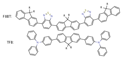
Figure 1: Chemical structures of F8BT and TFB oligomers.

As an application of our approach we consider the decay of an excitonic state into a charge-separated state at the interface between two semiconducting polymer phases (TFB) and (F8BT). The chemical structures of these are given in Fig. 1. Such materials have been extensively studied for their potential in organic light-emitting diodes and organic photovoltaics Morteani et al. (2003); Morteani et al. (2005a); Dhoot et al. (2004); Morteani et al. (2004); Morteani et al. (2005b); Sreearunothai et al. (2006). At the phase boundary, the material forms a type-II semiconductor heterojunction with the off-set between the valence bands of the two materials being only slightly more than the binding energy of an exciton placed on either the TFB or F8BT polymer. As a result, an exciton on the F8BT side will dissociate to form a charge-separated (exciplex) state at the interface. Morteani et al. (2005b); Morteani et al. (2003, 2004); Silva et al. (2001); Stevens et al. (2001)

$${\rm F8BT}^{*}:{\rm TFB}\longrightarrow{\rm F8BT}^{-}:{\rm TFB}^{+}.$$

Ordinarily, such type II systems are best suited for photovoltaic rather than LED applications However, LEDs fabricated from phase-segregated 50:50 blends of TFB:F8BT give remarkably efficient electroluminescence efficiency due to secondary exciton formation due the back-reaction

$${\rm F8BT}^{-}:{\rm TFB}^{+}\longrightarrow{\rm F8BT}^{*}:{\rm TFB}.$$

as thermal equilbrium between the excitonic and charge-transfer states is established. This is evidenced by long-time emission, red-shifted relative to the emission from the exciplex, accounting for nearly 90% of the integrated photo-emission.

Here we consider only two electronic levels corresponding to

$$|XT\rangle={\rm F8BT}^{*}:{\rm TFB}\,\,\&\,\,|CT\rangle={\rm F8BT}^{-}:{\rm TFB}^{+}.$$

We take the vertical energies for these two states as $\epsilon_{CT}=2.019$eV and $\epsilon_{XT}=2.306$ eV. As was shown in Ref. Khan et al. (2004); Bittner et al. (2005); Karabunarliev et al. (2001, 2000), in poly-fluorene based systems, there are essentially two phonon bands that are coupled strongly to the electronic degrees of freedom as evidenced by their presence as vibronic features in the vibronic emission spectra. Within our model these are represented by two narrow sine-shaped bands. The first, centered about 97.40 cm^-1 with a width of 10.16 cm^-1, accounts for the low-frequency torsional motions while the second, higher frequency band centered at 1561.64 cm^-1 with width 156.30 cm^-1 accounts for the C=C ring-stretching modes. These primitive modes are entirely localized on one chain or the other. The vibronic couplings within the model were determined by comparison between the Franck-Condon peaks of the predicted and observed spectra of the system Khan et al. (2004). We studied this model system before using several different approachesRamon and Bittner (2007, 2006); Tamura et al. (2008); Pereverzev and Bittner (2006). As before, we consider the initial excitonic state as being prepared in the $|XT\rangle$ state corresponding to the photoexcitation of the F8BT polymer. The full set of parameters for the model may be obtained as the supplemental material of Ref. Pereverzev and Bittner (2006).

III.1 Contributions from Coupling Modes

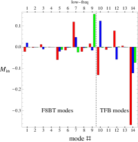
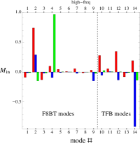
Figure 2: Projection of the three coupling modes onto the primitive modes for the model heterojunction system. (a) Projection onto low frequency torsional modes and (b) projection on to the higher frequency C=C modes included in the model. Red, Blue, and Green indicate the contributions from coupling modes 1,2, and 3 respectively.

First, we examine the effect of mode-projection on the model Hamiltonian describing the heterojunction. Following the mode-projection, the 28 primitive modes reduce to three coupling modes with frequencies $\omega_{s}=1587.61$cm^-1, 1625.07 cm^-1, and 1637.22 cm^-1 respectively. The projection of these modes onto the primitive basis is shown in Fig. 2. These projected modes involve contributions from both the high and low frequency phonon bands, although the dominant contributions come from the higher frequency phonon band. Furthermore, since the primitive modes are localized to the individual molecular units, we can comment that the first coupling mode $\omega_{1}=1587.61$ cm^-1 (shown in red in Fig. 2) involves contributions from both molecules, while the other two modes (shown in blue and green, in Fig. 2 respectively) are dominated by local contributions coming from either the F8BT chain or the TFB chain.

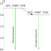
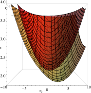
Figure 3: a.) Energy level diagram showing relevant electronic states and corresponding vertical excitation energies. b.) A slices through the 3-dimensional Born-Oppenheimer potential energy surface for the model heterojunction dimer. Here, $x_{3}$ is fixed at the global minima (corresponding to the CT diabatic curve),

In Fig. 3 we show some details of the potential energy surface generated by our model Hamiltonian. Fig. 3a shows the position of the two relevant electronic states corresponding to the emissive excitonic state and the weakly emissive exciplex state. Within the model, there does exist an intermediate charge-transfer state that is energetically close to the XT state. We recently explored the and energetics Ramon and Bittner (2007) and dynamical Tamura et al. (2008) implications of such dark exciplex states using quantum chemical and numerically exact quantum propagation. In the initial transfer, the intermediate state (for this system at least) plays a minimal role with most of the population being transferred directly from the XT to CT. However, it does play a role in the back transfer process. In Fig. 3b we give a slice along along one of the projected mode coordinates ($x_{2}$) keeping $x_{3}$ fixed at the energy minimum of the CT state. The slice where $x_{1}$ is at the CT energy minimum indicates that the system is nearly in the “barrierless” regime for electron transfer as suggested by the experimental observations.Morteani et al. (2003)

III.2 Population Relaxation

We now examine the dynamical ramifications of the mode projection scheme for the system following excitation to the XT state. In Ref. Pereverzev and Bittner (2006) we showed that to second-order in the electron/phonon couplings, non-Markovian contributions to the population decay can be included within a time-convolutionless form of the master equation (TCLME)

$$\frac{dP_{\alpha}(t)}{dt}=\sum_{\beta}W_{\alpha\beta}(t)P_{\beta}(t)-\sum_{\beta}W_{\beta\alpha}(t)P_{\alpha}(t).$$ (21)

in which the time dependent rates $W_{\alpha\beta}(t)$ are given by

$$W_{\beta\alpha}(t)=2Re\int_{0}^{t}d\tau\langle M_{\alpha\beta}M_{\beta\alpha}(\tau)\rangle e^{-i(\tilde{\epsilon}_{\alpha}-\tilde{\epsilon}_{\beta})\tau},$$ (22)

where

$$\langle M_{\alpha\beta}M_{\beta\alpha}(\tau)\rangle={\rm Tr}\left(M_{\alpha\beta}M_{\beta\alpha}(\tau)\rho_{eq}\right).$$ (23)

is the autocorrelation of the off-diagonal coupling operator in the Heisenberg representation for the canonical ensemble $\rho_{eq}$. The explicit form of $C_{\alpha\beta}(\tau)=\langle M_{\alpha\beta}M_{\beta\alpha}(\tau)\rangle$ is complicated and lengthy and the reader is referred to the original work for its details. Provided that the correlation function $C_{\alpha\beta}(t)\rightarrow 0$ at long times, the golden-rule rate is given by

$$W_{\beta\alpha}^{g.r.}=\lim_{t\rightarrow\infty}W_{\beta\alpha}(t).$$ (24)

At long times when the rates become constant the TCLME preserves both positivity and detailed balance. However, at intermediate times one can obtain negative rates depending upon the spectral density of the couplingPereverzev and Bittner (2006).

In Fig. 4 and Fig. 5 we compare the results of various approximate decoupling scheme with results obtained without using the decoupling. As a first approximation, we disregard all the bath modes and their couplings to the system modes. Thus, only the terms describing electronic degrees of freedom and the three $c$-modes are kept. Clearly, this can only be a good approximation if in the transformed Hamiltonian (Eq. 2) the coupling between the system modes and bath modes is weak. For the case at hand, this proves to be a reasonable approximation for a short time dynamics but a poor approximation for longer times as the population never relaxes from the initial state. This indicates that the coupling between the $c$-modes and residual $r$ modes is sufficiently strong and cannot be ignored.

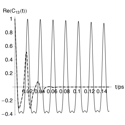
Figure 4: The real part of the correlation function $C_{13}(t)$ for the fully-coupled 28 modes model (solid gray) and reduced 3 (solid black) and 6 (dashes) mode decoupled models. Here we use a temperature of $T=298$K.

The picture is completely different if we perform independent unitary transformations within each of the two phonon bands of our model. In this case the electronic degrees of freedom are coupled to a total of six $c$-modes, three for each phonon band. Within the TCLME formalism, the computed population decay is virtually indistinguishable from the fully coupled (28-mode) case even out to long times.

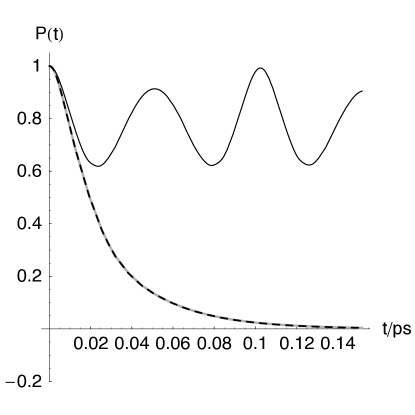
Figure 5: The TCLME population of the excited state as a function of time for the fully-coupled 28 modes model (solid gray) and reduced 3 (solid black) and 6 (dashes) mode decoupled models. $T=298$K.

In Ref. Tamura et al. (2007, 2006) the same model was investigated by using different truncations of the Mori chain with the time evolution of the multi-dimensional electron/phonon wavefunction was propagated using the numerically exact multi-configuration time-dependent Hartree (MCTDH) methodWorth et al. ; Beck et al. (2000). The results obtained there are qualitatively similar to ours in that too severe of a truncation produces no relaxation and that both high and low frequency contributions are needed to affect the fission of the exciton.

IV Discussion

Here we have presented one very straightforward and essentially universal procedure for reducing the complexity of a quantum dynamical simulation of a multi-dimensional multi-state system by reducing the number of normal modes directly interacting with the electronic system. Splitting all the normal modes into two groups allows one to apply different levels of theory to each of these groups. In particular, one can expect that as far as the electronic dynamics goes that the modes that are directly coupled to the electronic degrees of freedom are more important and showed be treated by more exact methods while the residual modes can be treated semi-classically as a bath. Such approximations should certainly be justified if the system modes are weakly coupled to the bath modes. We showed that rather then using the minimum number of system modes it is possible to adjust the number of the system modes to reduce their coupling the bath modes. It would be desirable to develop an unambiguous procedure for choosing the optimum number of modes that are still few in number and at the same time weakly coupled to the residual modes. So far the only unambiguous criteria that we have is that doing transformations of the type of Eq. (3) within the groups of modes with near-degenerate frequencies generally leads to the weak system-bath mode coupling. In particular, in case of complete degeneracy, the system and bath modes are completely decoupled.

Appendix A

Consider the linear transformations

$$X_{i} = \sum_{j}M_{ij}x_{j},$$ (25)

$$P_{i} = \sum_{j}(\widetilde{M}^{-1})_{ij}p_{j},$$ (26)

where $M_{ij}$ are the elements of an arbitrary real invertible matrix ${\bf M}$. In this appendix we will show that these transformations are equivalent to the following unitary transformations of operators $x_{i}$ and $p_{i}$

$$X_{i}=U^{-1}x_{i}U,\qquad P_{i}=U^{-1}p_{i}U,$$ (27)

and, therefore, transformations in Eqs. (26) are canonical even though they are not orthogonal.

By virtue of the singular value decomposition theorem any invertible real matrix $\bf M$ can be written as

$${\bf M}={\bf O}_{1}{\bf D}\widetilde{{\bf O}}_{2},$$ (28)

where ${\bf O}_{1}$ and ${\bf O}_{2}$ are orthogonal matrices and ${\bf D}$ is a positive definite diagonal matrix. It is sufficient to show that that there is a unitary transformation corresponding to each of these matrices. Then the unitary transformation corresponding to ${\bf M}$ will be a product of these transformations. Consider the orthogonal matrices first. They can have a determinant of either $1$ or $-1$. If the determinant of an orthogonal matrix is positive it corresponds rotations in the multi-dimensional coordinate space. Let us show that in can be represented by the following unitary transformation of $x_{i}$ and $p_{i}$

$$X_{i}=U_{o}^{-1}x_{i}U_{o},\qquad P_{i}=U_{o}^{-1}p_{i}U_{o},$$ (29)

where

$$U_{o}=\exp\bigg{(}-\frac{i}{2}\sum_{ij}A_{ij}(p_{i}x_{j}+x_{j}p_{i})\bigg{)}$$ (30)

and ${\bf A}$ is a real anti-symmetric matrix. The explicit effect of the unitary transformation 29 can be calculated by introducing an auxiliary operator

$$U_{o}(\xi)=\exp\bigg{(}-\frac{i}{2}\sum_{ij}A_{ij}(p_{i}x_{j}+x_{j}p_{i})\xi\bigg{)}.$$ (31)

Consider the auxiliary coordinate and momentum operators

$$X_{i}(\xi)=U_{o}^{-1}(\xi)x_{i}U_{o}(\xi),\qquad P_{i}(\xi)=U_{o}^{-1}(\xi)p_{i}U_{o}(\xi).$$ (32)

Differentiating $X_{i}(\xi)$ and $P_{i}(\xi)$ with respect to $\xi$ and using the commutations relations between coordinates and momenta we obtain

$$\frac{dX_{i}(\xi)}{d\xi}=\sum_{j}A_{ij}X_{j}(\xi),\qquad\frac{dP_{i}(\xi)}{d\xi}=\sum_{j}A_{ij}P_{j}(\xi).$$ (33)

Solving the last two equations subject to the initial conditions $X_{i}(0)=x_{i}$ and $P_{i}(0)=p_{i}$ and bearing in mind that $X_{i}=X_{i}(1)$, $P_{i}=P_{i}(1)$ we have

$$X_{i}=\sum_{j}\left(e^{A}\right)_{ij}x_{j},\qquad P_{i}=\sum_{j}\left(e^{A}\right)_{ij}p_{j}.$$ (34)

Since any orthogonal matrix with determinant $1$ can be written as an exponential of an anti-symmetric matrix we can reproduce any orthogonal matrix in Eq. 34 by a suitable choice of $\bf A$. Thus, any orthogonal transformation with determinant $1$ can be represented by a unitary transformation of the form of Eq. (29). Let us now show that there exists a suitable unitary transformation of $x_{i}$ and $p_{i}$ if the determinant of either of the orthogonal matrices in Eq. 28 is negative. Any orthogonal matrix with the determinant of $-1$ can be written as a product of an arbitrary orthogonal matrix with the determinant of $-1$ and an orthogonal matrix with the determinant of $1$

$$O_{-1}=O_{-1}\widetilde{O^{\prime}}_{-1}{O^{\prime}}_{-1}=O^{\prime\prime}_{1}{O^{\prime}}_{-1}.$$ (35)

The case of the positive determinant orthogonal matrix was considered above. Therefore, we can choose a simple orthogonal matrix with determinant $-1$ for ${O^{\prime}}_{-1}$ and show that there is a corresponding unitary transformation. A simple choice is a diagonal matrix one of whose diagonal elements is equal to $-1$ and the rest are equal to $1$. Its action corresponds to the space inversion for one of the oscillators and has the following unitary realization

$$X_{i}=U_{q}^{-1}x_{i}U_{q},\qquad P_{i}=U_{q}^{-1}p_{i}U_{q}$$ (36)

with

$$U_{q}=\exp\left(i\pi\left(\frac{p^{2}_{i}}{2}+\frac{x^{2}_{i}}{2}\right)\right).$$ (37)

Finally matrix ${\bf D}$ being a positive definite diagonal matrix corresponds to the rescaling of the coordinate and momentum operators of the following form

$$X_{i}=e^{B_{i}}x_{i},\qquad P_{i}=e^{-B_{i}}p_{i}$$ (38)

and also has a unitary realization as

$$X_{i}=U_{s}^{-1}x_{i}U_{s},\qquad P_{i}=U_{s}^{-1}p_{i}U_{s},$$ (39)

where

$$U_{s}=\exp\left(-i\sum_{i}\frac{B_{i}}{2}\left(x_{i}p_{i}+p_{i}x_{i}\right)\right)$$ (40)

Thus , we showed that transformations in Eqs. (26) can be viewed as unitary transformations of operators $x_{i}$ and $p_{i}$.

Appendix B

In this appendix we will show that it is possible to transform Eq. (2) to the form in which there are still $n_{s}$ system modes but each of the operators $|a\rangle\langle b|+|b\rangle\langle a|$ (for $a\neq b$) and $|a\rangle\langle a|$ interacts with its own single mode. We consider the case of a two-level system, generalizations to higher-level systems are trivial. Consider the case of two-level electronic system and, therefore, three system modes ($n_{s}=3$). Let us show that it can be transformed into

$$H = \sum_{a=1}^{2}\epsilon_{a}|a\rangle\langle a|+Y_{1}|1\rangle\langle 1|+Y_{2}|2\rangle\langle 2|+Y_{3}\Big{(}|1\rangle\langle 2|+|2\rangle\langle 1|\Big{)}$$ (41)

$$+\sum_{i=1}^{3}\sum_{j=4}^{N}G_{ij}Y_{i}X_{j}+\sum_{i,j=1}^{3}\frac{U_{ij}{\Pi}_{i}{\Pi}_{j}}{2}+\sum_{i,j=1}^{3}\frac{V_{ij}{Y}_{i}{Y}_{j}}{2}$$

$$+ \sum_{i=4}^{N}\frac{{P}_{i}^{2}}{2}+\sum_{i=4}^{N}\frac{{\omega^{\prime}}_{i}^{2}{X}_{i}^{2}}{2},$$

where we have written the electron-phonon interaction part explicitly. Thus, only one mode is directly responsible for the electronic transitions. Eq. 41 can be obtained from Eq. 2 by the following non-orthogonal transformation of coordinate and momentum operators in the space of system modes

$$Y_{i}=\sum_{i=j=1}^{3}L_{ij}X_{j},\qquad\Pi_{i}=\sum_{i=j=1}^{3}(\widetilde{L}^{-1})_{ij}P_{j}.$$ (42)

This is a special case of the coordinate transformations we used earlier. Here $L_{ij}$ are elements of the following $3\times 3$ matrix ${\bf L}$

$${\bf L}=\pmatrix{g_{111}&g_{112}&g_{113}\cr g_{221}&g_{222}&g_{223}\cr g_{121}&g_{122}&g_{123}\cr}$$ (43)

and $(\widetilde{M}^{-1})_{ij}$ denote matrix elements of the inverse of the transpose of ${\bf L}$. Matrix elements $U_{ij}$ and $V_{ij}$ in Eq. 41 are given by

$$U_{ij}=\sum_{k=1}^{3}\widetilde{L}_{ki}\widetilde{L}_{kj},\qquad V_{ij}=\sum_{k=1}^{3}{\omega^{\prime}_{k}}^{2}(L^{-1})_{ki}(L^{-1})_{kj},$$ (44)

and

$$G_{ij}=\sum_{k=1}^{3}\gamma^{\prime}_{kj}(L^{-1})_{ki}.$$ (45)

We would like to stress again here that even though matrix ${\bf L}$ is non-orthogonal operators $Y_{i}$ and $\Pi_{i}$ are unitarily equivalent to, respectively, $X_{i}$ and $P_{i}$, and therefore, Hamiltonian (41) is unitarily equivalent to Hamiltonian (2).