LPTENS-08/27

FOLLOWING THE PATH OF CHARM:
NEW PHYSICS AT THE LHC

JOHN ILIOPOULOS

Laboratoire de Physique Théorique

de L’Ecole Normale Supérieure

75231 Paris Cedex 05, France

Talk presented at the ICTP on the occasion of the Dirac medal award ceremony
Trieste, 27/03/08

It is a great honour for me to speak on this occasion and I want to express my gratitude to the Abdus Salam International Centre for Theoretical Physics as well as the Selection Committee of the Dirac Medal. It is also a great pleasure to be here with Luciano Maiani and discuss the consequences of our common work with Sheldon Glashow on charmed particles [1]. I will argue in this talk that the same kind of reasoning, which led us to predict the opening of a new chapter in hadron physics, may shed some light on the existence of new physics at the as yet unexplored energy scales of LHC.

The argument is based on the observation that precision measurements at a given energy scale allow us to make predictions concerning the next energy scale. It is remarkable that the origin of this observation can be traced back to 1927, the two fundamental papers on the interaction of atoms with the electromagnetic field written by Dirac, which are among the cornerstones of quantum field theory. In the second of these papers [2] Dirac computes the scattering of light quanta by an atom $\gamma(k_{1})+A_{i}\rightarrow\gamma(k_{2})+A_{f}$, where $A_{i}$ and $A_{f}$ are the initial and final atomic states, respectively. He obtains the perturbation theory result:

$$H_{fi}=\Sigma_{j}\frac{H^{1}_{fj}H^{1}_{ji}}{E_{i}-E_{j}}$$ (1)

where $H$ are the amplitudes. For the significance of the rhs, Dirac notes: “…The scattered radiation thus appears as a result of the two processes $i\rightarrow j$ and $j\rightarrow f$, one of which must be an absorption, the other an emission, in neither of which the total proper energy is even approximately conserved.” This is the crux of the matter: In the calculation of a transition amplitude we find contributions from states whose energy may put them beyond our reach. The size of their contribution decreases with their energy, see (1), so, the highest the precision of our measurements, the further away we can see.

Let me illustrate the argument with two examples, one with a non-renormalisable theory and one with a renormalisable one. A quantum field theory, whether renormalisable or not, should be viewed as an effective theory valid up to a given scale $\Lambda$. It makes no sense to assume a theory for all energies, because we know already that at very high energies entirely new physical phenomena appear (example: quantum gravity at the Planck scale). The first example is the Fermi four-fermion theory with a coupling constant $G_{F}\sim 10^{-5}GeV^{-2}$. It is a non-renormalisable theory and, at the $n$th order of perturbation, the $\Lambda$ dependence of a given quantity $A$ is given by:

$$A^{(n)}=C_{0}^{(n)}(G_{F}\Lambda^{2})^{n}+C_{1}^{(n)}G_{F}(G_{F}\Lambda^{2})^{n-1}+C_{2}^{(n)}G_{F}^{2}(G_{F}\Lambda^{2})^{n-2}+....$$ (2)

where the $C_{i}$’s are functions of the masses and external momenta, but their dependence on $\Lambda$ is, at most, logarithmic. Perturbation theory breaks down obviously when $A^{(n)}\sim A^{(n+1)}$ and this happens when $G_{F}\Lambda^{2}\sim 1$. This gives a scale of $\Lambda\sim 300$GeV as an upper bound for the validity of the Fermi theory. Indeed, we know today that at 100GeV the $W$ and $Z$ bosons change the structure of the theory. But, in fact, we can do much better than that [3]. Weak interactions violate some of the conservation laws of strong interactions, such as parity and strangeness. The absence of such violations in precision measurements will tell us that $G_{F}\Lambda^{2}\sim\epsilon$ with $\epsilon$ being the experimental precision. The resulting limit depends on the value of the $C$ coefficient for the quantity under consideration. In this particular case it turned out that, under the assumption that the chiral symmetry of strong interactions is broken only by terms transforming like the quark mass terms, the coefficient $C_{0}^{(n)}$ for parity and/or strangeness violating amplitudes vanishes and no new limit is obtained [4]. However, the second order coefficient $C_{1}^{(n)}$ contributes to flavour changing neutral current transitions and the smallness of the $K_{1}-K_{2}$ mass difference, or the $K^{0}_{L}\rightarrow\mu^{+}+\mu^{-}$ decay amplitude, give a limit of $\Lambda\sim 3$GeV before new physics should appear. The new physics in this case turned out to be the charmed particles [1]. We see in this example that the scale $\Lambda$ turned out to be rather low and this is due to the non-renormalisable nature of the effective theory which implies a power-law behaviour of the radiative corrections on $\Lambda$.

The second example in which new physics has been discovered through its effects in radiative corrections is the well-known “discovery” of the $t$ quark at LEP, before its actual production at Fermilab. The effective theory is now the Standard Model, which is renormalisable. In this case the dependence of the radiative corrections on the scale $\Lambda$ is, generically, logarithmic and the sensitivity of the low energy effective theory on the high scale is weak (there is an important exception to this rule for the Standard Model which we shall see presently). In spite of that, the discovery was made possible because of the special property of the Yukawa coupling constants in the Standard Model to be proportional to the fermion mass. Therefore, the effects of the top quark in the radiative corrections are quadratic in $m_{t}$. The LEP precision measurements were able to extract a very accurate prediction for the top mass.

I claim that we are in a similar situation with the precision measurements of the Standard Model. Our confidence in this model is amply justified on the basis of its ability to accurately describe the bulk of our present day data and, especially, of its enormous success in predicting new phenomena. All these spectacular successes are in fact successes of renormalised perturbation theory. Indeed what we have learnt was how to apply the methods which had been proven so powerful in quantum electrodynamics, to other elementary particle interactions. The remarkable quality of modern High Energy Physics experiments, mostly at LEP, but also elsewhere, has provided us with a large amount of data of unprecedented accuracy. All can be fit using the Standard Model with the Higgs mass as the only free parameter. Let me show some examples: Figure 1 indicates the overall quality of such a fit. There are a couple of measurements which lay between 2 and 3 standard deviations away from the theoretical predictions, but it is too early to say whether this is accidental, a manifestation of new physics, or the result of incorrectly combining incompatible experiments.

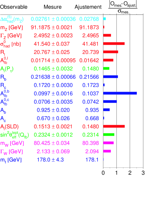
Figure 1: Various physical quantities measured and computed.

Another impressive fit concerns the strong interaction effective coupling constant as a function of the momentum scale (Figure 2). This fit already shows the importance of taking into account the radiative corrections, since, in the tree approximation, $\alpha_{s}$ is obviously a constant. Similarly, Figure 3 shows the importance of the weak radiative corrections in the framework of the Standard Model. Because of the special Yukawa couplings, the dependence of these corrections on the fermion masses is quadratic, while it is only logarithmic in the Higgs mass. The $\epsilon$ parameters are designed to disentangle the two. The ones we use in Figure 3 are defined by:

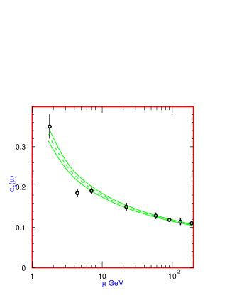
Figure 2: The variation of $\alpha_{s}$ with the momentum scale. The renormalisation group prediction and the experimental points.

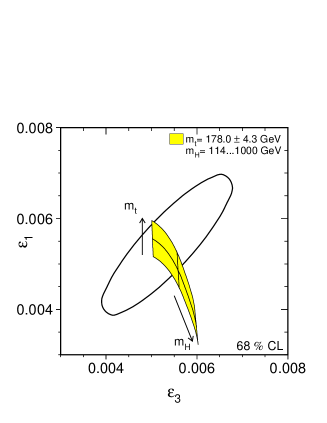
Figure 3: The importance of the Standard Model radiative corrections. The arrows show how the prediction moves when we vary $m_{t}$ and $m_{H}$, in particular if we use the most recent lower value for $m_{t}$.

$$\epsilon_{1}=\frac{3G_{F}m_{t}^{2}}{8\sqrt{2}\pi^{2}}-\frac{3G_{F}m_{W}^{2}}{4\sqrt{2}\pi^{2}}\tan^{2}\theta_{W}\ln\frac{m_{H}}{m_{Z}}+...$$ (3)

$$\epsilon_{3}=\frac{G_{F}m_{W}^{2}}{12\sqrt{2}\pi^{2}}\ln\frac{m_{H}}{m_{Z}}-\frac{G_{F}m_{W}^{2}}{6\sqrt{2}\pi^{2}}\ln\frac{m_{t}}{m_{Z}}+...$$ (4)

where the dots stand for subleading corrections. As you can see, the $\epsilon$ s vanish in the absence of weak interaction radiative corrections, in other words, $\epsilon_{1}=\epsilon_{3}=0$ are the values we get in the tree approximation of the Standard Model but after having included the purely QED and QCD radiative corrections. We see clearly in Figure 3 that this point is excluded by the data. The latest values for these parameters are $\epsilon_{1}=5.4\pm 1.0$ and $\epsilon_{3}=5.34\pm 0.94$ [5].

Using all combined data we can extract the predicted values for the Standard Model Higgs mass which are given in Figure 4. The data clearly favour a low mass ($\leq 200$ GeV) Higgs, although, this prediction may be less solid than what Figure 4 seems to indicate.

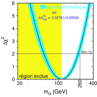
Figure 4: The predicted values for the Standard Model Higgs mass using all available data. The shaded region is excluded by direct searches.

The main conclusion I want to draw from this comparison can be stated as follows:

Looking at all the data, from low energies to the Tevatron, we have learnt that perturbation theory is remarkably successful, outside the specific regions where strong interactions are important.

Let me explain this point better: At any given model with a coupling constant $g$ we expect to have a weak coupling region $g\ll 1$, in which weak coupling expansions, such as perturbation theory, are reliable, a strong coupling region with $g\gg 1$, in which strong coupling expansions may be relevant, and a more or less large gray region $g\sim 1$, in which no expansion is applicable. The remarkable conclusion is that this gray area appears to be extremely narrow. And this is achieved by an enlargement of the area in which weak coupling expansion applies. The perturbation expansion is reliable, not only for very small couplings, such as $\alpha_{em}\sim 1/137$, but also for moderate QCD couplings $\alpha_{s}\sim 1/3$, as shown in Figure 2. This is extremely important because without this property no calculation would have been possible. If we had to wait until $\alpha_{s}$ drops to values as low as $\alpha_{em}$ we could not use any available accelerator. Uncalculable QCD backgrounds would have washed out any signal. And this applies, not only to the Tevatron and LHC, but also to LEP. We can illustrate this observation using a qualitative argument first introduced by F. Dyson. He noted that in a field theory like QED, the contribution of the $2n$-th order perturbation term to a physical amplitude $A^{(2n)}$ grows with $n$ roughly as

$$A^{(2n)}\sim\alpha^{n}(2n-1)!!$$ (5)

where $\alpha$ is (the square of) the coupling constant. Again, perturbation theory will break down when $A^{(2n)}\sim A^{(2n+2)}$ which gives

$$2n+1\sim\alpha^{-1}$$ (6)

This leaves a comfortable margin for QED but leaves totally unexplained the successes of QCD at moderate energies.

A global view of the weak and strong coupling regions is given in Figure 5 which shows the $R$-ratio, i.e. the $e^{+}+e^{-}$ total cross section to hadrons normalised to that of $e^{+}+e^{-}\rightarrow\mu^{+}+\mu^{-}$ as a function of the centre-of-mass energy. The lowest order perturbation value for this ratio is a constant, equal to $\Sigma Q_{i}^{2}$, the sum of the squares of the quark charges accessible at this energy. We see clearly in this Figure the areas of applicability of perturbation theory: At very low energies, below 1 GeV, we are in the strong coupling regime characterised by resonance production. The strong interaction effective coupling constant becomes of order one (we can extrapolate from Figure 2), and perturbation breaks down. However, as soon as we go slightly above 1 GeV, $R$ settles to a constant value and it remains such except for very narrow regions when new thresholds open. In these regions the cross section is again dominated by resonances and perturbation breaks down. But these areas are extremely well localised and threshold effects do not spread outside these small regions.

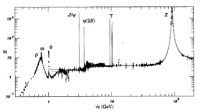
Figure 5: The ratio $R$ of $e^{+}+e^{-}$ total cross section to hadrons normalised to that of $e^{+}+e^{-}\rightarrow\mu^{+}+\mu^{-}$ as a function of the centre-of-mass energy.

In this talk I want to exploit this observational fact and argue that the available precision tests of the Standard Model allow us to claim with confidence that new physics will be unravelled at the LHC, although we have no unique answer on the nature of this new physics. The argument assumes the validity of perturbation theory and it will fail if the latter fails. But, as we just saw, perturbation theory breaks down only when strong interactions become important. But new strong interactions do imply new physics.

The key is again the Higgs boson. As we explained above, the data favour a low mass Higgs. However, the opposite cannot be excluded, first because it depends on the subset of the data one is looking at, and, second, because the analysis is done taking the minimal Standard Model.

Given this result, let us see what, if any, are the theoretical constraints. The Standard Model Higgs mass is given, at the classical level, by $m_{H}^{2}=2\lambda v^{2}$, with $v$ the vacuum expectation value of the Higgs field. $v$ is fixed by the value of the Fermi coupling constant $G_{F}/\sqrt{2}=1/(2v^{2})$ which implies $v\approx$246 GeV. Therefore, any constraints will come from the allowed values of $\lambda$. A first set of such constraints is given by the classical requirement:

$$1>\lambda>0~{}~{}~{}~{}\Rightarrow~{}~{}~{}~{}m_{H}<400-500GeV$$ (7)

The lower limit for $\lambda$ comes from the classical stability of the theory. If $\lambda$ is negative the Higgs potential is unbounded from below and there is no ground state. The upper limit comes from the requirement of keeping the theory in the weak coupling regime. If $\lambda\geq 1$ the Higgs sector of the theory becomes strongly interacting and we expect to see plenty of resonances and bound states rather than a single elementary particle.

Going to higher orders is straightforward, using the renormalisation group equations. The running of the effective mass is determined by that of $\lambda$. Keeping only the dominant terms and assuming $t=\log(v^{2}/\mu^{2})$ is small ($\mu\sim v$), we find

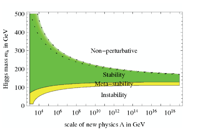
Figure 6: Bounds on the Higgs mass.

$$\frac{d\lambda}{dt}=\frac{3}{4\pi^{2}}[\lambda^{2}+3\lambda h_{t}^{2}-9h_{t}^{4}+...]$$ (8)

where $h_{t}$ is the coupling of the Higgs boson to the top quark. The dots stand for less important terms, such as the other Yukawa couplings to the fermions and the couplings with the gauge bosons. This equation is correct as long as all couplings remain smaller than one, so that perturbation theory is valid, and no new physics beyond the standard model becomes important. Now we can repeat the argument on the upper and lower bounds for $\lambda$ but this time taking into account the full scale dependence $\lambda(\mu)$. We thus obtain for the Higgs mass an upper bound given by the requirement of weak coupling regime ($\lambda(\mu)<1$) all the way up to the scale $\mu$, and a lower bound by the requirement of vacuum stability ($\lambda(\mu)>0$), again up to $\mu$. Obviously, the bounds will be more stringent the larger the assumed value of $\mu$. Figure 6 gives the allowed region for the Higgs mass as a function of the scale for scales up to the Planck mass. We see that for small $\mu\sim 1$TeV, the limits are, essentially, those of the tree approximation equation (7), while for $\mu\sim M_{P}$ we obtain only a narrow window of allowed masses 130GeV$<m_{H}<$200GeV, remarkably similar to the experimental results.

This analysis gives the first conclusion: If perturbation theory remains valid, in other words, if we have no new strong interactions, there exists at least one, relatively light, Higgs boson:

Conclusion 1: The absence of a light Higgs boson implies New Physics.

Here “heavy Higgs” is not clearly distinguished from “no-Higgs”, because a very heavy Higgs, above 1 TeV, is not expected to appear as an elementary particle. As we explained above, this will be accompanied by new strong interactions. A particular version of this possibility is the “Technicolor” model, which assumes the existence of a new type of fermions with strong interactions at the multi-hundred-GeV scale. The role of the Higgs is played by a fermion-antifermion bound state. “New Physics” is precisely the discovery of a completely new sector of elementary particles. Other strongly interacting models can and have been constructed. The general conclusion is that a heavy Higgs always implies new forces whose effects are expected to be visible at the LHC.

The possibility which seems to be favoured by the data is the presence of a “light” Higgs particle. In this case new strong interactions are not needed and, therefore, we can assume that perturbation theory remains valid. But then we are faced with a new problem. The Standard Model is a renormalisable theory and the dependence on the high energy scale is expected to be only logarithmic. This is almost true, but with one notable exception: The radiative corrections to the Higgs mass are quadratic in whichever scale $\Lambda$ we are using. The technical reason is that $m_{H}$ is the only parameter of the Standard Model which requires, by power counting, a quadratically divergent counterterm. The gauge bosons require no mass counterterm at all because they are protected by gauge invariance and the fermions need only a logarithmic one. The physical reason is that, if we put a fermion mass to zero we increase the symmetry of the model because now we can perform chiral transformations on this fermion field. Therefore the massless theory will require no counterterm, so the one needed for the massive theory will be proportional to the fermion mass and not the cut-off. In contrast, putting $m_{H}=0$ does not increase the symmetry of the model. As a result the effective mass of the Higgs boson will be given by

$$(m_{H}^{2})_{eff}=m_{H}^{2}+C\alpha_{eff}\Lambda^{2}$$ (9)

where $C$ is a calculable numerical coefficient of order one and $\alpha_{eff}$ some effective coupling constant. In practice it is dominated by the large coupling to the top quark. The moral of the story is that the Higgs particle cannot remain light unless there is a precise mechanism to cancel this quadratic dependence on the high scale. This is a particular aspect of a general problem called “scale hierarchy”. The only known mechanism which reconciles a light Higgs and a high value of the scale $\Lambda$ with the validity of perturbation theory is supersymmetry. In this case the Higgs mass is protected against the quadratic corrections of eq. (9) because it behaves like the mass of the companion fermion which, as we just said, receives only logarithmic corrections. It is closest in spirit to the charm mechanism, in the sense that a heavy effective cut-off is made compatible with the low energy data by the presence of new particles. The alternative is to have a low value of $\Lambda$, i.e. new physics, at a low scale. The models with large compact extra dimensions enter into this category. This brings us to our second conclusion:

Conclusion 2: A light Higgs boson is unstable without new physics.

Both conclusions are good news for LHC. But the time for speculations is coming to an end. The LHC is coming. Never before a new experimental facility had such a rich discovery potential and never before was it loaded with so high expectations.

References

- [1] S.L. Glashow, J. Iliopoulos and L. Maiani, Phys. Rev. D2 (1970) 1285.
- [2] P.A.M. Dirac, Proc. Roy. Soc. A114 (1927) 710.
- [3] B.L. Joffe and E.P. Shabalin, Yadern Fiz. 6 (1967) 828 (Soviet J. Nucl. Phys. 6 (1968) 603); Z. Eksp. i Teor. Fiz. Pis’ma U Red. 6 (1967) 978 (Soviet. Phys. JETP Lett. 6 (1967) 390).
- [4] C. Bouchiat, J. Iliopoulos and J. Prentki, Nuov. Cim. 56A (1968) 1150; J. Iliopoulos, Nuov. Cim. 62A (1969) 209.
- [5] G. Altarelli, Private Communication.