Bound states in $N=2$ Liouville theory with boundary
and
Deep throat D-branes

Abstract

We exhibit bound states in the spectrum of non-compact D-branes in $N=2$ Liouville conformal field theory. We interpret these states in the study of D-branes in the near-horizon limit of Neveu-Schwarz five-branes spread on a topologically trivial circle. We match semi-classical di-electric and repulsion effects with exact conformal field theory results and describe the fate of D-branes hitting NS5-branes. We also show that the bound states can give rise to massless vector and hyper multiplets in a low-energy gauge theory on D-branes deep inside the throat.

Laboratoire de Physique Théorique , Ecole Normale Supérieure,
24 rue Lhomond, F–75231 Paris Cedex 05, France

1 Introduction

Liouville conformal field theory plays a central role in two-dimensional gravity and string theory as well as in our present understanding of conformal field theories with continuous spectrum. When rendered $N=2$ supersymmetric, it becomes a building block for supersymmetric string backgrounds. We further study $N=2$ superconformal Liouville theory with boundary in this paper, and concentrate in particular on exhibiting bound states on non-compact branes.

In a separate development, an intuitive description of large parts of gauge theory physics has been given in terms of brane set-ups (see e.g. [1][2][3]). We believe it is an interesting task to study descriptions of brane set-ups that are valid at all energy scales. It further brings to bare string theory techniques in gauge theory physics and vice versa. For instance, one may suspect that world-sheet $N=2$ holomorphy will turn out to be a useful alternative tool to analyze space-time physics.

The analysis of D-branes in Neveu-Schwarz five-brane backgrounds [4] was revisited in [5] using the tools developed to solve non-rational conformal field theories. It was argued how to realize brane set-ups [1] in terms of boundary conformal field theories (see also [6][7]).

In this paper we wish to analyze in more detail than in [5] how a D-brane behaves in the close neighborhood of NS5-branes. We will study a particular set-up where the NS5-branes are evenly arranged on a topologically trivial circle. We will see how target space physics is coded in intricate properties of $N=2$ Liouville theory with boundary. In section 2 we lay bare the relevant properties of $N=2$ Liouville theory with boundary, which include new relations between formal boundary states as well as the appearance of bound states in boundary spectra. In section 3 we review briefly the bulk conformal field theory. We construct D-branes in the full superstring theory in section 4, and analyze their spectrum. In section 5 we give a space-time interpretation of the conformal field theory results of section 2. In particular we show the appearance of light bound states on the world-volume of non-compact D-branes as they approach NS5-branes. We also describe the cutting of D-branes as they hit NS5-branes. We analyze the gauge theory excitations living deep inside the triply scaled throat in section 6. In section 7 we discuss a special case with more symmetry allowing us to make a crosscheck, and we conclude with a summary and suggestions for further developments in section 8. Various detailed calculations are gathered in the appendices for the benefit of the indefatigable reader.

2 Addition relations and bound states on the boundary

We first analyze aspects of $N=2$ Liouville theory with boundary (see e.g. [7][8][9][10][11]). We will derive new addition relations between boundary states, and show the appearance of normalizable boundary vertex operators as bound states on non-compact branes.

2.1 Unitary representations of the $N=2$ superconformal algebra

We take the central charge of our $N=2$ Liouville model to be

$$c=3+\frac{6}{k}$$ (1)

where $k$ is a strictly positive integer. States in $N=2$ Liouville theory can be organized in representations of the $N=2$ superconformal algebra. The characters of the representations can be obtained as coset characters from the $N=1$ superconformal extension of an $SL(2,\mathbb{R})$ current algebra [12] after gauging a compact $U(1)$ subalgebra. In the following we use the $SL(2,\mathbb{R})$ quantum numbers to label the representations of the $N=2$ superconformal algebra. After descent in the NS-sector, the primary state with Casimir and $U(1)$ labels $(J,m)$ has conformal dimension $h$ and $U(1)_{R}$ charge $Q$ determined by the formulas:

$$h=-\frac{J(J-1)}{k}+\frac{m^{2}}{k},\qquad Q=\frac{2m}{k}$$ (2)

We take the R-charge $Q$ to be quantized such that $2m\in\mathbb{Z}$.

We have different families of unitary representations:

• Continuous characters ($0\leq J\leq\frac{1}{2}$ or $J=\frac{1}{2}+iP$, $P\in\mathbb{R}^{+}$; $m$ generic):

  $$ch_{c}(J,m;\tau,z)=q^{-\frac{J(J-1)}{k}+\frac{m^{2}}{k}-\frac{1}{4k}}y^{\frac{2m}{k}}\frac{\theta_{3}(\tau,z)}{\eta^{3}(\tau)}$$ (3)

  These representations have no null vectors. The parent $SL(2,\mathbb{R})$ representation has a spectrum for a compact generator which is doubly infinite.

• Discrete representations ($J=\frac{1}{2},1,\dots,\frac{k+1}{2}$ ; $m=J+r$, $r\in\mathbb{Z}$ ):

  $$ch_{d}(J,r;\tau,z)=q^{-\frac{(J-1/2)^{2}}{k}+\frac{(J+r)^{2}}{k}}y^{\frac{2(J+r)}{k}}\frac{1}{1+yq^{1/2+r}}\frac{\theta_{3}(\tau,z)}{\eta^{3}(\tau)}$$ (4)

  These have one null vector and are inherited from a representation of $SL(2,\mathbb{R})$ with semi-infinite spectrum. When $r$ is negative, the conformal dimension and R-charge of the primary are given by formulae (2) with $\tilde{m}=J+r-k/2$ and $\tilde{J}=(k+2)/2-J$ (see [9]).

• Identity representation ($J=0$; $m\in\mathbb{Z}$):

  $$ch_{\mathbb{I}}(m;\tau,z)=q^{-\frac{1}{4k}+\frac{m^{2}}{k}}y^{\frac{2m}{k}}\frac{1-q}{(1+yq^{\frac{1}{2}+m})(1+y^{-1}q^{\frac{1}{2}-m})}\frac{\theta_{3}(\tau,z)}{\eta^{3}(\tau)}$$ (5)

  This representation has two null vectors. It descends from the trivial representation of the $SL(2,\mathbb{R})$ algebra.

We hope the notations are sufficiently intuitive and refer to [12] and [9] for further details.

The chiral and anti-chiral rings of the $N=2$ superconformal field theory form interesting subsectors of the theory. The chiral ring is generated by the operators that satisfy $h=\frac{Q}{2}$. In the anti-chiral ring, the relation $h=-\frac{Q}{2}$ is satisfied. We find a chiral primary state in the discrete character when $r=0$, and an anti-chiral primary state in the discrete character when $r=-1$ (see [9]). The identity character with $m=0$ contains the identity operator ($h=Q=0$) which is both chiral and anti-chiral.

Interpreted as a $\sigma$-model, $N=2$ Liouville theory has a curved non-compact target space. States in continuous representations with $J=\frac{1}{2}+iP$ propagate to infinity. The momentum in the curved non-compact direction is denoted by $P$. States in discrete or identity representations are bound states.

The characters of the ${N}=2$ superconformal algebra satisfy the following identity [7]:

$$ch_{c}(J=0,m=0)=ch_{I}(m=0)+ch_{d}(J=\frac{k}{2},r=0)+ch_{d}(J=1,r=-1).$$ (6)

as well as the identity

$$ch_{c}(J=\frac{1}{2},m=\frac{1}{2})=ch_{d}(J=\frac{1}{2},r=0)+ch_{d}(J=\frac{k+1}{2},r=0).$$ (7)

These identities can be viewed as generalizations of the identities between discrete, continuous and the trivial representations of $SL(2,\mathbb{R})$. One can write down such an identity for any continuous character, if there exists a discrete or a finite dimensional representation with the same quantum numbers. These additional addition relations are either spectral flowed from (6) and (7) (see later), or involve non-unitary characters.

Note that the case $k=1$ is special. In that case, we can combine the two relations (6) and (7) to obtain an identity involving only the identity and continuous characters:

$$ch_{c}^{k=1}(J=0,m=0)=ch_{I}^{k=1}(m=0)+ch_{c}^{k=1}(J=\frac{1}{2},m=\frac{1}{2}).$$ (8)

2.2 Spectral flow and extended characters

When we simultaneously change boundary conditions on all fermionic operators of the $N=2$ superconformal algebra (such that they pick up a phase as one goes around a world-sheet circle), we spectral flow the $N=2$ algebra. After one unit of spectral flow, we recuperate the original boundary conditions. This operation acts on the quantum numbers $(J,m)$ of a given state as $(J,m)\to(J,m+1)$.

We define the extended ${N}=2$ superconformal algebra as being generated by the usual ${N}=2$ generators together with the operator implementing $k$ units of spectral flow. For applications in superstring theory and to simplify the modular properties of the characters, it is convenient to classify the states in representations of the extended algebra. We define the following extended characters:

$$Ch_{c}(J,m;\tau,z)=\sum_{n\in\mathbb{Z}}ch_{c}(J,m+kn;\tau,z)$$ (9)

$$Ch_{d}(J,r;\tau,z)=\sum_{n\in\mathbb{Z}}ch_{d}(J,r+kn;\tau,z)$$ (10)

$$Ch_{I}(m;\tau,z)=\sum_{n\in\mathbb{Z}}ch_{\mathbb{I}}(m+kn;\tau,z)$$ (11)

The quantum numbers $m$ and $r$ labeling the extended characters are defined modulo $k$. The behavior of these extended characters under modular transformations is given in appendix A. We can perform spectral flow on both sides of the identities (6) and (7) (by any amount) and obtain new identities. In particular, the character identities (6) and (7) are valid for the extended characters as well:

$$Ch_{c}(J=0,m=r)=Ch_{\mathbb{I}}(m=r)+Ch_{d}(J=\frac{k}{2},r)+Ch_{d}(J=1,r-1).$$ (12)

$$Ch_{c}(J=\frac{1}{2},m=\frac{1}{2}+r)=Ch_{d}(J=\frac{1}{2},r)+Ch_{d}(J=\frac{k+1}{2},r).$$ (13)

2.3 Boundary states

We consider A-type branes in ${N}=2$ Liouville theory (see e.g. [7][9][11]). The boundary state associated to a brane $B$ is written as:

$$|B\rangle=\int_{P=0}^{\infty}\sum_{2m=0}^{2k-1}\psi^{B}_{c}(P,m)|P,m\rangle\rangle_{c}+\sum_{2J=2}^{k}\sum_{2m=0}^{2k-1}\psi^{B}_{d}(J,m)|J,m\rangle\rangle_{d}$$ (14)

The definition of the continuous and discrete Ishibashi states $|P,m\rangle\rangle_{c}$ and $|J,m\rangle\rangle_{d}$, as well as the one-point couplings to the discrete operators $\psi^{B}_{d}(J,m)$, are given in appendix A. In the bulk of the paper, we focus on the one-point functions of the continuous operators $\psi^{B}_{c}(P,m)$.

The identity brane $|0\rangle_{\mathbb{I}}$ whose self-overlap is the extended identity character $Ch_{\mathbb{I}}(m=0)$ (in the boundary channel) has the following one-point function:

$$\Psi^{\mathbb{I}}_{0}(P,m) = \nu^{iP}\frac{\Gamma(\frac{1}{2}+iP+m)\Gamma(\frac{1}{2}+iP-m)}{\Gamma(1+2iP)\Gamma(\frac{2iP}{k})}.$$ (15)

The parameter $\nu$ is related to the coefficient $\mu$ of the bulk Liouville potential as $\nu=\mu^{2/k}$ (see [8][11]). The branes whose overlap with the identity brane $|0\rangle_{\mathbb{I}}$ are one of the extended characters (9), (10) or (11) are specified by the one-point functions:

• Continuous brane $|\hat{P},\hat{m}\rangle_{c}$ :

  $$\psi_{\hat{P},\hat{m}}^{c}(P,m) = \nu^{iP}\frac{2}{k}e^{-2\pi i\frac{2m.2\hat{m}}{2k}}\cos(4\pi P\hat{P}/k)\frac{\Gamma(1-2iP)\Gamma(\frac{-2iP}{k})}{\Gamma(\frac{1}{2}-iP+m)\Gamma(\frac{1}{2}-iP-m)}.$$ (16)

  We can take the definition to apply to boundary states with $\hat{P}$ purely imaginary as well. As long as we stay within the bounds $0\leq i\hat{P}\leq\frac{1}{2}$ the overlap with the identity brane $|0\rangle_{\mathbb{I}}$ is the continuous character with real $\hat{J}=\frac{1}{2}+i\hat{P}$, $0\leq\hat{J}\leq 1/2$, which remains a unitary representation of the superconformal algebra.

• Discrete brane $|\hat{J},\hat{r}\rangle_{d}$ :

  $$\psi^{d}_{\hat{J},\hat{r}}(P,m) = \nu^{iP}\frac{1}{2k}e^{-2\pi i\frac{2(\hat{J}+\hat{r}).2m}{2k}}\frac{\Gamma(1-2iP)\Gamma(-2i\frac{P}{k})}{\Gamma(\frac{1}{2}-iP+m)\Gamma(\frac{1}{2}-iP-m)}$$ (17)

  $$\times\frac{\cosh\left(2\pi\frac{P(2\hat{J}-1)}{k}\right)+(-1)^{2m}\cosh\left(2\pi\frac{P(k-2\hat{J}+1)}{k}\right)}{|\cosh\pi(P+im)|^{2}}.$$

• Identity brane $|\hat{m}\rangle_{\mathbb{I}}$ :

  $$\Psi^{\mathbb{I}}_{\hat{m}}(P,m)=\nu^{iP}e^{-2\pi i\frac{2m.2\hat{m}}{2k}}\frac{\Gamma(\frac{1}{2}+iP+m)\Gamma(\frac{1}{2}+iP-m)}{\Gamma(1+2iP)\Gamma(\frac{2iP}{k})}.$$ (19)

The Cardy condition has been checked for the continuous and identity branes. For the discrete branes, this condition is not satisfied in general [7][9][13]. We show in appendix A that discrete characters generically appear with non-integer and/or negative multiplicity in the overlap of two discrete branes. That indicates that the discrete boundary states are inconsistent.

2.4 Brane addition relations

The modular bootstrap approach suggests that the characters identities (12) and (13) can be extended to the full boundary states. That is the case for example in bosonic Liouville theory (see [14][16]). There is also a known example in supersymmetric Liouville theory at level $k=1$ (see [17]). We propose the relations ($\hat{r}\in\mathbb{Z}$):

$$|\hat{J}=0,\hat{r}\rangle_{c} = |\hat{r}\rangle_{\mathbb{I}}+|k/2,\hat{r}\rangle_{d}+|1,-1+\hat{r}\rangle_{d}$$ (20)

$$|\hat{P}=0,1/2+\hat{r}\rangle_{c} = |1/2,\hat{r}\rangle_{d}+|k/2+1/2,\hat{r}\rangle_{d}.$$ (21)

The labels of the brane correspond to the extended character that appears when computing the annulus partition function for boundary operators between the brane and the identity brane $|0\rangle_{\mathbb{I}}$. After some $\Gamma$-function and trigonometric gymnastics, it can be shown that the one-point functions for these branes indeed satisfy the corresponding addition relations. Moreover, the identities hold for the discrete part of the Cardy states as well.

Since the boundary states for individual discrete branes do not pass the Cardy check, we cannot view these addition relations as identities between consistent boundary states. Nevertheless, we will see in section 5 that these relations code semi-classical properties of D-branes in string theory.

As a side-remark we note that in the special case $k=1$, we get the brane addition relations of [17]:

$$|\hat{J}=0,\hat{r}\rangle_{c}^{k=1} = |\hat{J}=1/2,1/2+\hat{r}\rangle_{c}^{k=1}+|\hat{r}\rangle_{\mathbb{I}}^{k=1}.$$ (22)

In this case, the addition relation is one between boundary states that pass the Cardy check individually.

2.5 Bound states on non-compact branes

We will now investigate more closely the first addition relation (20). If one computes the self overlap of the right-hand side of the relation (20), one will obtain states in discrete and in the identity representations. These states are bound states, localized on the world-volume of the brane. Their conformal dimension can lie below the continuum of boundary vertex operators. In this section we wish to understand the appearance of these bound states in the self overlap of the continuous brane on the left-hand side of (20). To that end, we will compute the overlap of two continuous branes ${}_{c}\langle\hat{P}_{1},\hat{m}_{1}|\mathrm{prop}|\hat{P}_{2},\hat{m}_{2}\rangle_{c}$, where “prop” represents the bulk (cylinder) propagator. Then we will study what happens when we continue $\hat{P}_{1}$ and $\hat{P}_{2}$ to $\frac{i}{2}$ (i.e. $\hat{J}_{1}$ and $\hat{J}_{2}$ to zero). This analysis is inspired by similar analyses in bosonic Liouville theory [15][16], and in supersymmetric Liouville theory at level $k=1$ [17].

We start from the definition of the continuous branes (14), (16). The continuous branes do not couple to discrete bulk operators. The overlap of the two branes gives in the bulk channel:

$$Z_{1,2} = {}_{c}\langle\hat{P}_{1},\hat{m}_{1}|\mathrm{prop}|\hat{P}_{2},\hat{m}_{2}\rangle_{c}=\int_{0}^{\infty}dP\sum_{2m\in Z_{2k}}\frac{4}{k^{2}}e^{2\pi i\frac{2m(2\hat{m}_{1}-2\hat{m}_{2})}{2k}}\cos\left(\frac{4\pi P\hat{P}_{1}}{k}\right)\cos\left(\frac{4\pi P\hat{P}_{2}}{k}\right)$$ (23)

$$\frac{\cos\pi(-iP+m)\cos\pi(iP+m)}{\sinh(2\pi P)\sinh(\frac{2\pi P}{k})}Ch_{c}^{closed}(P,m)$$

We obtain the partition function in the loop channel via a modular transformation:

$$Z_{1,2} = \int_{0}^{\infty}dP\frac{1}{k}\sum_{\epsilon_{1},\epsilon_{2}=\pm 1}\cosh\left(2\pi P\left(1+2i\epsilon_{1}\frac{\hat{P}_{1}}{k}+2i\epsilon_{2}\frac{\hat{P}_{2}}{k}\right)\right)\frac{1}{\sinh(2\pi P)\sinh(\frac{2\pi P}{k})}$$ (24)

$$\int_{-\infty}^{\infty}dP^{\prime}e^{\frac{4\pi iPP^{\prime}}{k}}Ch^{open}_{c}(P^{\prime},\hat{m}_{1}-\hat{m}_{2})$$

$$+ \int_{0}^{\infty}dP\frac{2}{k}\sum_{\epsilon_{2}=\pm 1}\cosh\left(2\pi P\left(2i\frac{\hat{P}_{1}}{k}+2i\epsilon_{2}\frac{\hat{P}_{2}}{k}\right)\right)\frac{1}{\sinh(2\pi P)\sinh(\frac{2\pi P}{k})}$$

$$\int_{-\infty}^{\infty}dP^{\prime}e^{\frac{4\pi iPP^{\prime}}{k}}Ch^{open}_{c}\left(P^{\prime},\hat{m}_{1}-\hat{m}_{2}+\frac{k}{2}\right)$$

Now we would like to write the boundary partition function $Z_{1,2}$ in a more explicit form as an integral over boundary operators with a given spectral density:

$$Z_{1,2} = \int_{P^{\prime}=-\infty+i\Delta}^{\infty+i\Delta}\rho_{1}(P^{\prime};\hat{P}_{1},\hat{P}_{2})Ch_{c}^{open}(P^{\prime},\hat{m}_{1}-\hat{m}_{2})$$ (25)

$$+\int_{P^{\prime}=-\infty+i\Delta}^{\infty+i\Delta}\rho_{2}(P^{\prime};\hat{P}_{1},\hat{P}_{2})Ch_{c}^{open}\left(P^{\prime},\hat{m}_{1}-\hat{m}_{2}+\frac{k}{2}\right).$$

Notice the imaginary shift $\Delta$ in the integration contour. This shift is needed for the following reason: in order to make the necessary exchange of the bulk and boundary momentum integrals, we need the integral over the bulk momentum $P$ at fixed boundary momentum $P^{\prime}$ to be convergent. Looking at the integrand in (24), we identify two possible divergences at $P=0$ and $P\to\infty$. Firstly, the integral is always divergent when the bulk momentum $P$ goes to zero. Notice that the behavior of the integrand close to $P=0$ is universal: it does not depend on the brane parameters $\hat{P}_{1}$, $\hat{P}_{2}$. It is an infrared divergence due to the non-compactness of the target space. We can cure the divergence either by considering a relative spectral density (subtracting a reference spectral density with fixed value of the brane parameters), or by removing the pole by hand. Secondly, the bulk momentum integral may still diverge due to the ultraviolet integration region. A prescription to cure this divergence [15] is to lift the integration contour for the boundary momentum $P^{\prime}$ by giving it a sufficient imaginary part $\Delta$. Then the integrand will decay exponentially at large momentum $P$, and we will be able to exchange the order of integration.

Let’s compute the necessary shift of the contour $\Delta$. At large momentum $P$, the integrand in the first two lines of equation (24) behaves as: $\exp\left(\frac{2\pi P}{k}(2i\epsilon_{1}\hat{P}_{1}+2i\epsilon_{2}\hat{P}_{2}-1+2iP^{\prime})\right)$. The integrand in the last two lines of equation (24) is always less divergent. We deduce that we need to shift the integration contour when $2Im(\hat{P}_{1})+2Im(\hat{P}_{2})\geq 1$. We recall that we took the imaginary parts of $\hat{P}_{1,2}$ to be positive. The imaginary part we give to the boundary momentum $P^{\prime}$ is:

$$\Delta=\max\left(0\,,\,Im(\hat{P}_{1})+Im(\hat{P}_{2})-\frac{1}{2}+\epsilon\right)$$ (26)

with $0<\epsilon\ll 1$. Since we have the inequality $0\leq Im(\hat{P}_{1}),Im(\hat{P}_{2})\leq\frac{1}{2}$, we need both $\hat{P}_{1}$ and $\hat{P}_{2}$ imaginary to have a non-zero shift (or one of them equal to $i/2$, in which case $\Delta=\epsilon$).

After giving a sufficiently large imaginary part to the boundary momentum (which breaks parity symmetry in $P^{\prime}$), we find the following densities of boundary operators:

$$\rho_{1}(P^{\prime};\hat{P}_{1},\hat{P}_{2}) = \int_{0}^{\infty}dP\frac{1}{k}\sum_{\epsilon_{1},\epsilon_{2}=\pm 1}\frac{\cosh\left(2\pi P\left(1+2i\epsilon_{1}\frac{\hat{P}_{1}}{k}+2i\epsilon_{2}\frac{\hat{P}_{2}}{k}\right)\right)}{\sinh(2\pi P)\sinh(\frac{2\pi P}{k})}e^{\frac{4\pi iPP^{\prime}}{k}}$$

$$\rho_{2}(P^{\prime};\hat{P}_{1},\hat{P}_{2}) = \int_{0}^{\infty}dP\frac{2}{k}\sum_{\epsilon_{2}=\pm 1}\frac{\cosh\left(2\pi P\left(2i\frac{\hat{P}_{1}}{k}+2i\epsilon_{2}\frac{\hat{P}_{2}}{k}\right)\right)}{\sinh(2\pi P)\sinh(\frac{2\pi P}{k})}e^{\frac{4\pi iPP^{\prime}}{k}}.$$ (27)

The densities $\rho_{1}$ and $\rho_{2}$ are functions of the boundary momentum $P^{\prime}$ as well as the two brane parameters $\hat{P}_{1}$ and $\hat{P}_{2}$. For given brane parameters, one can extend these functions over the whole complex plane in $P^{\prime}$, and identify their poles. One can then bring the $P^{\prime}$ integral back to the real line (in order for the continuous part of the spectrum to correspond to continuous characters), pick up the poles crossed in the process, and identify them as isolated contributions to the partition function.

To analyze the pole structure of the densities of states $\rho_{1}$ and $\rho_{2}$, we can rewrite these densities as the derivatives of phase shifts. We can perform the rewriting in terms of the q-gamma function $\Gamma_{b}(x)$. It is defined as (see e.g. [18]):

$$\log\Gamma_{b}(x) = \int_{0}^{\infty}\frac{dt}{t}\frac{e^{-xt}-e^{Qt/2}}{(1-e^{-bt})(1-e^{-t/b})}-\frac{(Q-2x)^{2}}{8e^{t}}-\frac{Q-2x}{t}$$ (28)

where $Q=b+b^{-1}$. This function has poles at $x=-mb-nb^{-1}$, where $m$ and $n$ are positive integers. With $b=\sqrt{k}$ and $t=2\pi p$, we can write $\rho_{1}$ and $\rho_{2}$ in terms of q-gamma functions as :

$$\rho_{1}(P^{\prime};\hat{P}_{1},\hat{P}_{2}) = \frac{1}{2\pi i}\sum_{\epsilon_{1},\epsilon_{2}=\pm 1}\frac{\partial}{\partial P^{\prime}}\left[\log\Gamma_{\sqrt{k}}\left(\frac{-iP^{\prime}+\frac{1}{2}+i\epsilon_{1}\hat{P}_{1}+i\epsilon_{2}\hat{P}_{2}}{\sqrt{k}}\right)\right.$$ (29)

$$\left.+\log\Gamma_{\sqrt{k}}\left(\frac{-iP^{\prime}+\frac{1}{2}+k+i\epsilon_{1}\hat{P}_{1}+i\epsilon_{2}\hat{P}_{2}}{\sqrt{k}}\right)\right]$$

$$\rho_{2}(P^{\prime};\hat{P}_{1},\hat{P}_{2}) = \frac{2}{2\pi i}\sum_{\epsilon_{1},\epsilon_{2}=\pm 1}\frac{\partial}{\partial P^{\prime}}\left[\log\Gamma_{\sqrt{k}}\left(\frac{-iP^{\prime}+\frac{1}{2}+\frac{k}{2}+i\epsilon_{1}\hat{P}_{1}+i\epsilon_{2}\hat{P}_{2}}{\sqrt{k}}\right)\right].$$ (30)

We note that we subtracted a universal part in the densities that does not depend on the parameters of the branes $\hat{P}_{1}$ and $\hat{P}_{2}$. The subtraction regularizes the bulk infrared divergence due to the infinite volume of the target space.

We can identify which poles are met when we bring back the $P^{\prime}$ integration contour to the real axis (cf. figure 1). For the density $\rho_{1}$, the poles are at:

$$-iP^{\prime} = -1/2-n-km+i\epsilon_{1}\hat{P}_{1}+i\epsilon_{2}\hat{P}_{2}$$

$$-iP^{\prime} = -1/2-k-n-km-i\epsilon_{1}\hat{P}_{1}-i\epsilon_{2}\hat{P}_{2}$$ (31)

whereas for the density $\rho_{2}$, we have poles at:

$$-iP^{\prime}=-1/2-k/2-n-km-i\epsilon_{1}\hat{P}_{1}-i\epsilon_{2}\hat{P}_{2}$$ (32)

where $\epsilon_{1},\ \epsilon_{2}=\pm 1$, and $m$ and $n$ are positive integers. Given that $0\leq Im(\hat{P}_{1}),Im(\hat{P}_{2})\leq\frac{1}{2}$, there is only one pole in the spectral density $\rho_{1}$ that will be crossed as we shift the boundary momentum contour to the real axis: the one from the first series in equation (2.5) with $m=n=0$ and $\epsilon_{1}=\epsilon_{2}=-1$. The residue for this pole is $+1$. The contour of the integral with the spectral density $\rho_{2}$ will not cross a pole when $k$ is greater than one.

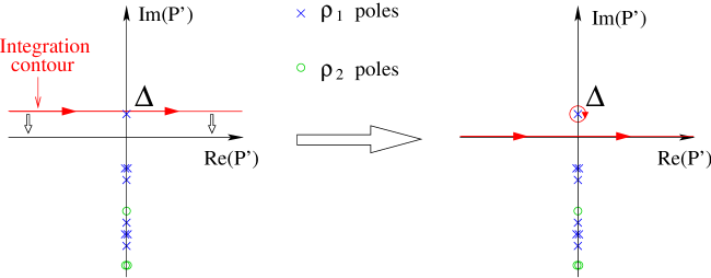
Figure 1: As we shift back to the real axis the integration contour for the boundary momentum, we pick up an additional contribution from a pole in the density of states $\rho_{1}$. It gives an isolated contribution to the partition function.

Eventually we can write down the annulus partition function in an explicit form:

• When $\Delta=0$:

  $$Z_{1,2} = \int_{P^{\prime}=-\infty}^{\infty}dP^{\prime}\rho_{1}(P^{\prime};\hat{P}_{1},\hat{P}_{2})Ch_{c}^{open}(P^{\prime},\hat{m}_{1}-\hat{m}_{2})$$ (33)

  $$+ \int_{P^{\prime}=-\infty}^{\infty}dP^{\prime}\rho_{2}(P^{\prime};\hat{P}_{1},\hat{P}_{2})Ch_{c}^{open}\left(P^{\prime},\hat{m}_{1}-\hat{m}_{2}+\frac{k}{2}\right)$$

• When $\Delta\neq 0$:

  $$Z_{1,2} = \int_{P^{\prime}=-\infty}^{\infty}dP^{\prime}\rho_{1}(P^{\prime};\hat{P}_{1},\hat{P}_{2})Ch_{c}^{open}(P^{\prime},\hat{m}_{1}-\hat{m}_{2})$$ (34)

  $$+ \int_{P^{\prime}=-\infty}^{\infty}dP^{\prime}\rho_{2}(P^{\prime};\hat{P}_{1},\hat{P}_{2})Ch_{c}^{open}\left(P^{\prime},\hat{m}_{1}-\hat{m}_{2}+\frac{k}{2}\right)$$

  $$+ Ch_{c}^{open}\left(P^{\prime}=\hat{P}_{1}+\hat{P}_{2}-\frac{i}{2},\hat{m}_{1}-\hat{m}_{2}\right)$$

Self-overlap of a continuous brane

Let’s examine the self-overlap of a continuous brane with parameters $(\hat{P},\hat{m})$. This is just a special case of the previous calculation when we take the values $\hat{P}=\hat{P}_{1}=\hat{P}_{2}$ and $\hat{m}=\hat{m}_{1}=\hat{m}_{2}$. So we obtain:

• When the brane parameter $\hat{P}$ is real, or between $0\leq Im(\hat{P})\ <\frac{1}{4}$:

  $${}_{c}\langle\hat{P},\hat{m}|\mathrm{prop}|\hat{P},\hat{m}\rangle_{c} = \int_{-\infty}^{\infty}dP^{\prime}\left(\rho_{1}(P^{\prime};\hat{P})Ch_{c}^{open}(P^{\prime},0)+\rho_{2}(P^{\prime};\hat{P})Ch_{c}^{open}\left(P^{\prime},\frac{k}{2}\right)\right)$$

• When the brane parameter is in the range $\frac{1}{4}<Im(\hat{P})\leq\frac{1}{2}$:

  $${}_{c}\langle\hat{P},\hat{m}|\mathrm{prop}|\hat{P},\hat{m}\rangle_{c} = \int_{-\infty}^{\infty}dP^{\prime}\left(\rho_{1}(P^{\prime};\hat{P})Ch_{c}^{open}(P^{\prime},0)+\rho_{2}(P^{\prime};\hat{P})Ch_{c}^{open}\left(P^{\prime},\frac{k}{2}\right)\right)$$ (36)

  $$+ Ch_{c}^{open}(J^{\prime}=1-2Im(\hat{P}),m=0)$$

An additional localized contribution appears starting at $Im(\hat{P})=\frac{1}{4}$ (namely, at half the momentum intercept caused by the linear dilaton). It contains relevant boundary operators, some of which have a conformal dimension below the continuum. At the value $Im(\hat{P})=\frac{1}{2}$ one of these operators becomes of conformal dimension zero. There the continuous character $Ch_{c}^{open}(\hat{J}=0,\hat{m}=0)$ splits into two discrete and one identity characters, according to the identity (12). If we would go further and give $\hat{P}$ an imaginary part greater than $1/2$, we would encounter characters of non-unitary representations.

We fulfilled our goal to compute the self-overlap of the continuous brane appearing on the left-hand side of the brane addition relation (20):

$${}_{c}\langle\hat{J}=0,\hat{m}|\mathrm{prop}|\hat{J}=0,\hat{m}\rangle_{c} = \int_{-\infty}^{\infty}dP^{\prime}\left(\rho_{1}(P^{\prime};\hat{P},\hat{P})Ch_{c}^{open}(P^{\prime},0)\right.$$ (37)

$$+\left.\rho_{2}(P^{\prime};\hat{P},\hat{P})Ch_{c}^{open}\left(P^{\prime},\frac{k}{2}\right)\right)$$

$$+ Ch_{\mathbb{I}}^{open}(0)+Ch_{d}^{open}(\frac{k}{2},0)+Ch_{d}^{open}(1,-1)$$

In appendix A it is shown that one obtains the same result for the self-overlap of the sum of branes on the right-hand side of equation (20). It is interesting to note that the way the correct multiplicity $+1$ for the discrete characters comes about in the algebraic calculation is via a multiplicity $+2$ from the overlap of identity brane with the discrete branes in the addition relation, and multiplicity $-1$ from the self-overlap of the sum of the discrete boundary states. That fact will be important later on.

Remarks

Firstly, as we noted in passing, the case $k=1$ needs to be studied separately. For $k=1$ and $\hat{J}=0$ the self-overlap picks up a pole in the density $\rho_{1}$ as before. Moreover, a pole in the spectral density $\rho_{2}$ coincides with the contour of integration in that case. That is due to a boundary infrared divergence. The integration can be regularized with a principal value prescription. Equivalently, we pick up the pole with weight a half (multiplied by the prefactor of $2$ associated to the density of states $\rho_{2}$). That leads to an extra contribution of a single continuous character with $J=1/2=m$ to the boundary spectrum. It implies that both discrete characters appear with multiplicity two in the self-overlap of the brane (37). The same conclusion is reached independently in appendix A. There it is shown that there are no discrete subtractions in this case. The upshot is an agreement with the discussion in [17] from both ways of calculating the self-overlap.

Secondly, we obtained the localized spectrum for generic level $k$ in two ways: on the one hand via the analytic continuation of the self-overlap, and on the other hand using the full identity and discrete boundary states including their coupling to the discrete Ishibashi states. We believe that provides a convincing crosscheck for these two procedures. This is important because it indicates that we should take the couplings of the discrete branes to discrete Ishibashi states seriously. It implies in particular that discrete branes do not (generically) pass the Cardy check.

We note that there may be exchange of discrete states between boundary states despite the fact that no pole appears in the density of exchanged bulk operators. Whether a discrete state is exchanged is determined by its coupling to both branes, and when these are non-zero, the contribution is weighted by the propagator. When one brane in the overlap is localized, those contributions correspond to the formal prescription to pick up possible poles and their residues in the bulk channel - why this is the case can be understood from the modular bootstrap (see e.g.[9]). That the prescription to pick up poles in the bulk channel only works when one of the two branes is localized seems related to the observation [19] that an analogue of the Verlinde formula in non-rational conformal field theories works well only in those cases.

In the dual boundary channel, it is the contour dictated by the precise boundary conditions that determine whether or not poles in the density of boundary operators contribute to the annulus amplitude [15].

2.6 Semi-classical analysis of the branes

We finalize this section by a few remarks on the semi-classic target space interpretation of the boundary conformal field theories. The semi-classical geometry has been described in e.g. [20][21][22][5] in some detail. We add a few extra remarks to those analyses that will be useful in the following.

When we think of ${N}=2$ Liouville theory as a two-dimensional $\sigma$-model, the associated trumpet target-space geometry is given by:

$$\left\{\begin{array}[]{l}ds^{2}=\alpha^{\prime}k\left(dr^{2}+\coth^{2}r\ d\psi^{2}\right)\\ e^{2\Phi}=\frac{e^{2\Phi_{0}}}{\sinh^{2}r}\end{array}\right.$$ (38)

The curvature radius of the geometry is $\sqrt{k\alpha^{\prime}}$. In the large $k$ limit, we can perform a useful semi-classical analysis. This analysis will break down close to $r=0$, where the geometry is singular (but the conformal field theory remains well-defined). The identity branes are located in that region.

Semi-classical D1-branes in the trumpet

Studying solutions that extremize the Dirac-Born-Infeld action for D1-branes in the background (38) (see e.g. [20]), one finds the following two-parameter family of branes:

$$\cosh(r)\sin(\psi-\psi_{0})=c$$ (39)

If $c>1$, we put $c\equiv\cosh r_{0}$. In this case the brane world-volume is limited to the region $r\geq r_{0}$. On the other hand, if $c\leq 1$, the brane extends over the whole space-time. When we go to radial infinity, the function $\sin(\psi-\psi_{0})$ goes to zero. So the branes described by the curve (39) have two anti-podal legs in the asymptotic region, in the angular directions $\psi=\psi_{0}$ and $\psi=\psi_{0}+\pi$.

These D1-branes are the semi-classical incarnations of the continuous and discrete branes as we will argue. We will also match the parameters $c$ and $\psi_{0}$ with the quantum numbers that label the Liouville branes.

Continuous branes

Let’s begin with the continuous branes $|\hat{P},\hat{m}\rangle_{c}$, with $\hat{P}$ real and strictly positive. It was argued in [22] that the T-dual D2 brane is doubly sheeted, and partially covers the cigar. We strengthen the arguments of [22]. First we notice that the parameter $\psi_{0}$ defines the position of the brane in the angular direction, so changing it should not change the self-overlap of the brane. Looking at equations (• ‣ 2.5) and (36), we deduce that the angle $\psi_{0}$ is a function of the quantum number $\hat{m}$ only. Moreover the two quantities $\psi_{0}$ and $\hat{m}$ are respectively defined modulo $2\pi$ and $2k$. We are lead to the identification:

$$\psi_{0}=2\pi\frac{\hat{m}}{k}-\frac{\pi}{2}$$ (40)

The additional (harmless) shift is chosen such that the angle $2\pi\frac{\hat{m}}{k}$ gives the direction of the tip of the brane (it is also the direction of an axis of symmetry for the brane). Now let’s consider the overlap of the brane $|\hat{P},\hat{m}\rangle_{c}$ with the identity brane $|\hat{m}\rangle_{\mathbb{I}}$. In the boundary channel, it is the continuous extended character $Ch_{c}(\hat{P},0)$. Thus all the open strings stretching between the two branes are massive. We deduce that the brane does not extend up to the horn at $r=0$, and the parameter $c$ of the semi-classical brane is greater than one. To compute the relation between the parameters $c$ and $\hat{P}$, we demand that the mass of a string be equal to its length times its tension. Equation (2) implies that the mass square of the lightest open string is $P^{2}/k\alpha^{\prime}$. On the other hand, a string stretching from the identity brane at $r=0$ up to the tip of the continuous brane at $r=r_{0}$ has proper length $r_{0}\sqrt{k\alpha^{\prime}}$, and mass $r_{0}\sqrt{k}/2\pi\sqrt{\alpha^{\prime}}$. Since $c=\cosh r_{0}$, we deduce that in the semi-classical limit:

$$c=\cosh\left(2\pi\frac{\hat{P}}{k}\right)$$ (41)

In the case where the brane label $\hat{P}$ is imaginary (and $\hat{J}$ is real), we expect the analytic continuation of the matching relation (41) to be valid:

$$c=\cos\left(2\pi\frac{2\hat{J}-1}{2k}\right).$$ (42)

In this case the brane extends up to the horn of the trumpet, and is made of two disconnected strands (see figure 2).

Discrete branes

The discrete branes have couplings to the continuous representations which are identical to those of the D2-branes covering the whole cigar [21]. This can be seen by rewriting:

$$\psi^{d}_{\hat{J},\hat{r}}(P,m) = \frac{1}{2\pi}\nu^{iP}e^{-2\pi i\frac{2m.2\hat{m}}{2k}}\Gamma(-2iP)\Gamma(1-2i\frac{P}{k})$$ (43)

$$\left(\frac{\Gamma(\frac{1}{2}+iP+m)}{\Gamma(\frac{1}{2}-iP+m)}e^{i\pi(\frac{1}{2}+\frac{1-2\hat{J}}{k})(2iP)}+\frac{\Gamma(\frac{1}{2}+iP-m)}{\Gamma(\frac{1}{2}-iP-m)}e^{-i\pi(\frac{1}{2}+\frac{1-2\hat{J}}{k})(2iP)}\right).$$

We identify the one-point functions after a T-duality transformation on the parameters. As for the continuous brane, the angular parameter $\psi_{0}$ is given by the quantum number $\hat{m}$:

$$\psi_{0}=2\pi\frac{\hat{m}}{k}-\frac{\pi}{2}$$ (44)

To precisely match the parameter $c$ of the semi-classical brane with the quantum numbers $\hat{J}$,$\hat{r}$ defining the discrete brane, we translate the semi-classical matching of the spectral density with the derivative of the reflection amplitude of [21] into our T-dual picture. We again obtain:

$$c=\cos\left(2\pi\frac{2\hat{J}-1}{2k}\right).$$ (45)

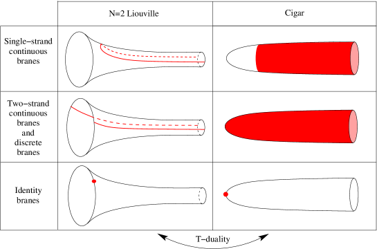
Figure 2: Semi-classical description of continuous, discrete and identity branes in $N=2$ Liouville theory, and their T-dual image in the cigar.

The number of branches

We note that the self-overlap of the discrete brane contains continuous representations with angular momentum $m=0$ and $m=k/2$ (cf. appendix A). Since the discrete branes have Dirichlet boundary conditions in the angular direction, we conclude (after appropriately normalizing) that open strings living on this brane have integer or half-integer winding number. This proves that the discrete branes have two anti-podal branches.

We may check this argument directly on the one-point function (43). We take the infrared limit by concentrating on the behavior of the one-point function for bulk operators with nearly zero momentum $P$. An analysis of the poles of the $\Gamma$-functions shows that the dominant couplings are to even momentum modes, which says that asymptotically we have two branches (that effectively halve the radius of the asymptotic circle, thus leading to only even momentum couplings).

The same arguments apply to the continuous branes which therefore also have two branches.

3 Neveu-Schwarz five-branes spread on a circle

We now want to use what we have learned about $N=2$ Liouville theory with boundary to study the behavior of D-branes close to NS5-branes. Our strategy will be to study the branes first in the T-dual coset conformal field theories, then to translate back the results into the NS5-brane background [5]. To that end, we briefly review the bulk string theory background and its T-duals [24][25].

3.1 The supergravity solution

Consider $k$ NS5-branes in type II string theory in flat space and stretching in the directions with coordinates $x^{\mu=0,1,\dots,5}$. They preserve sixteen supersymmetries. The coordinates of the transverse space are $x^{i=6,7,8,9}$. The back-reaction of the NS5-branes on flat space is coded in the string frame metric, the NSNS three-form $H_{(3)}$ and the dilaton $\Phi$:

$$\left\{\begin{array}[]{rcl}ds^{2}&=&\eta_{\mu\nu}dx^{\mu}dx^{\nu}+H\delta_{ij}dx^{i}dx^{j}\\ e^{2\Phi}&=&g_{s}^{2}\,H\\ H_{(3)}&=&\ast_{4}dH\end{array}\right.$$ (46)

where the harmonic function $H$ is specified in terms of the positions $x^{i}_{a}$ of the NS5-branes in transverse space:

$$H(x^{i}) = 1+\sum_{a=1}^{k}\frac{\alpha^{\prime}}{|x^{i}-x^{i}_{a}|^{2}},$$ (47)

and $\ast_{4}$ denotes the Hodge star operation in the four Euclidean transverse directions (with flat metric).

Figure 3: We consider $k$ NS5-branes extended in the directions $x^{0,1,..,5}$. They are evenly arranged on a circle of radius $\rho_{0}$, in the plane $x^{8}=x^{9}=0$.

We concentrate on $k$ NS5-branes whose positions are $k$ evenly spread points on a topologically trivial circle of radius $\rho_{0}$ in the $(x^{6},x^{7})$ plane (see figure 3). We introduce new coordinates $(r,\theta,\psi,\phi)$:

$$(x^{6},x^{7}) = \rho_{0}\cosh r\sin\theta\,(\cos\psi,\sin\psi)$$

$$(x^{8},x^{9}) = \rho_{0}\sinh r\cos\theta\,(\cos\phi,\sin\phi)\,.$$ (48)

where $r\in\mathbb{R}_{+}$, $0\leq\theta\leq\pi/2$, and $0\leq\phi,\psi\leq 2\pi$.
When we neglect world-sheet instanton corrections (or equivalently, spread the NS5-branes over the circle [26]), and take the double scaling limit [27]:

$$g_{s},\frac{\rho_{0}}{\sqrt{\alpha^{\prime}}} \to 0$$

$$\frac{\rho_{0}}{g_{s}\sqrt{\alpha^{\prime}}} \mbox{fixed},$$ (49)

the supergravity solution becomes:

$$\left\{\begin{array}[]{rcl}ds^{2}&=&dx^{\mu}dx_{\mu}+\alpha^{\prime}k\,\left[dr^{2}+d\theta^{2}+\frac{\tanh^{2}r\ d\phi^{2}+\tan^{2}\theta\ d\psi^{2}}{1+\tan^{2}\theta\tanh^{2}r}\right]\,,\\ e^{2\Phi}&=&\frac{g_{eff}^{2}}{\cosh^{2}r-\sin^{2}\theta}\,,\\ B&=&\frac{\alpha^{\prime}k}{1+\tan^{2}\theta\tanh^{2}r}\ d\phi\wedge d\psi\,,\end{array}\right.$$ (50)

where the effective string coupling constant is

$$g_{eff}=\frac{\sqrt{k\alpha^{\prime}}g_{s}}{\rho_{0}}.$$ (51)

This background is an exact coset conformal field theory, corresponding to a null gauging of $SU(2)\times SL(2,\mathbb{R})$ [28]. However it will be more convenient for us to use the exact conformal field theory description of a T-dual background. The exact conformal field theory encodes all world-sheet instanton corrections [29][30][5].

3.2 T-dual space-times and their conformal field theory description

We perform a T-duality along the angular direction $\phi$ and obtain the geometry:

$$\left\{\begin{array}[]{rcl}ds^{2}&=&dx^{\mu}dx_{\mu}+\alpha^{\prime}k\left[dr^{2}+\coth^{2}r\,\left(\frac{d\omega}{k}+d\psi\right)^{2}+d\theta^{2}+\mathrm{tan}^{2}\theta\,\left(\frac{d\omega}{k}\right)^{2}\right],\\ e^{2\Phi}&=&\frac{g_{eff}^{2}}{k}\ \frac{1}{\sinh^{2}r\cos^{2}\theta}\end{array}\right.$$ (52)

where $\omega$ is the coordinate T-dual to $\phi$. The bracketed part of this solution is a $\mathbb{Z}_{k}$ orbifold of the direct product of two known sigma-models, namely the trumpet (38), and the bell defined as:

$$\left\{\begin{array}[]{rcl}ds^{2}&=&\alpha^{\prime}k\left[d\theta^{2}+\tan^{2}\theta\,d\omega^{2}\right],\\ e^{2\Phi}&=&\frac{g_{\textsc{eff}}^{2}}{\cos^{2}\theta}.\end{array}\right.$$ (53)

The latter geometry is the target-space of the supercoset $\frac{SU(2)_{k}}{U(1)}$, also known as the $N=2$ minimal model of central charge $c=3-6/k$ (see [31] for a review). The trumpet geometry is more accurately described as $N=2$ Liouville theory with a momentum condensate.

In order to study the behavior of D-branes in the NS5-brane background (46), we will use the T-dual description (52). The conformal field theory describing the curved part of the background is the $\mathbb{Z}_{k}$ orbifold of the product $\left(\frac{SU(2)_{k}}{U(1)}\right)\,\times({N}=2\ \mathrm{Liouville})$ . The orbifold is the part of the GSO projection that renders the closed string $U(1)_{R}$ charges integer. To get a full description of the superstring background, we also have to take into account the six flat directions parallel to the NS5-brane world-volume. They are described by the ${N}=2$ conformal field theory of six free real bosons $X^{\mu=0,..,5}$ and six free real fermions $\psi^{\mu=0,..,5}$. We will work in light-cone gauge. In summary, the relevant critical conformal field theory describing the dynamics of strings in the background (52) is:

$$\left(\frac{\left(X^{\mu=2,..,5},\psi^{\mu=2,..,5}\right)\times\left(\frac{SU(2)_{k}}{U(1)}\right)\times\left({N}=2\,\,\mathrm{Liouville}\right)}{\mathbb{Z}_{k}^{GSO}}\right)/\mathbb{Z}_{2}^{GSO}$$ (54)

The product conformal field theory defines a particular non-compact Gepner model (see e.g. [32][33][34] for discussions of these models).

We can also perform T-duality along the isometric $\psi$ direction in the background (46) [5]. That would lead to the background described by the mirror dual of the conformal field theory (54). In this mirror description, the ${N}=2$ Liouville theory is replaced by the cigar [33][34].

4 D-branes in the coset conformal field theory

We will study D-branes in the full superstring theory by first constructing them in the product conformal field theory (54). In section 5 we re-interpret them in the Neveu-Schwarz five-brane background. We find more explicit realizations and important refinements of the proposals of [5].

4.1 D-branes in the minimal model and in flat space

The boundary states in the full conformal field theory (54) are the product of factors coming from Liouville theory, the minimal model and the free theory. We studied in detail the boundary states in Liouville theory in section 2. Here we review briefly the relevant boundary states in the minimal model and in flat space.

D-branes in flat space

D-branes in flat space are well-known. They induce Neumann or Dirichlet boundary conditions for the open strings, according to the directions in which they are extended. Let’s isolate two flat directions in space-time. They are described on the world-sheet by a free complex boson and fermion. It is convenient to bosonize the free fermion, to get a free compact boson at fermionic radius $\sqrt{2\alpha^{\prime}}$. The momentum for this compact boson is given by a $\mathbb{Z}_{4}$ integer $s$. If this quantum number is even, we are in the Neveu-Schwarz sector while if it is odd, we are in the Ramond sector. A D-brane extended in those two directions is labeled by a quantum number $\hat{s}$, and its one-point function is:

$$\psi^{N}_{\hat{s}}(s)=\frac{1}{\sqrt{2}}e^{-i\pi\frac{s\bar{s}}{2}}.$$ (55)

For a brane localized in those two directions, the one-point function is:

$$\psi^{D}_{\hat{s},\hat{x}^{\mu}}(s,k_{\mu})=\frac{1}{\sqrt{2}}e^{-i\pi\frac{s\bar{s}}{2}}e^{ik_{\mu}\hat{x}^{\mu}}.$$ (56)

In the previous formula, $k_{\mu}$ is the closed string momentum and $\hat{x}^{\mu}$ gives the position of the brane.

There is one subtlety when we work in the light-cone gauge: we have to put Dirichlet boundary conditions in the light-cone directions [35]. By a double Wick rotation, we can obtain branes extended in the time direction. The brane will be extended in at most four out of the six flat directions of (52). In the following we will consider for definiteness D-branes that fill four flat directions.

D-branes in the minimal model

D-branes in the $N=2$ minimal model have also been extensively studied (see e.g. [31]). A state in this theory is labeled by three quantum numbers: an $SU(2)_{k-2}$ spin $j=0,\frac{1}{2},...,\frac{k-2}{2}$, an angular momentum $n\in\mathbb{Z}_{2k}$, and a fermionic number $s\in\mathbb{Z}_{4}$. The D-branes with $A$-type boundary conditions are given by the one-point functions:

$$\psi_{\hat{j},\hat{n},\hat{s}}^{MM}(j,n,s)=\frac{1}{\sqrt{k}}\frac{\sin\left(\pi\frac{(2j+1)(2\hat{j}+1)}{k}\right)}{\sqrt{\sin\pi\frac{2j+1}{k}}}e^{i\pi\frac{n\hat{n}}{k}}e^{-i\pi\frac{s\hat{s}}{2}}.$$ (57)

The overlap of two branes is given in the open string channel by:

$$\langle\hat{j},\hat{n},\hat{s}|\mathrm{prop}|\hat{j}^{\prime},\hat{n}^{\prime},\hat{s}^{\prime}\rangle=\sum_{j}N_{\hat{j}\hat{j}^{\prime}}^{j}\chi^{open}(j,\hat{n}-\hat{n}^{\prime},\hat{s}-\hat{s}^{\prime})$$ (58)

where $\chi(j,n,s)$ are $N=2$ minimal model characters, and $N_{\hat{j}\hat{j}^{\prime}}^{j}$ are the $SU(2)_{k-2}$ fusion coefficients. These branes have a clear semi-classical description in the bell geometry (53), which is weakly curved at large $k$. They are described by the equation:

$$\sin(\theta)\sin(\omega-\omega_{0})=\sin(\theta_{0}).$$ (59)

The geometric parameters $\theta_{0}$ and $\omega_{0}$ are related to the brane quantum numbers $\hat{j}$ and $\hat{n}$ as [31]:

$$\theta_{0}=\frac{\pi}{2}-\frac{\pi(2\hat{j}+1)}{k}\ ,\quad\omega_{0}=\pi\frac{\hat{n}}{k}-\frac{\pi}{2}$$ (60)

The branes are oriented straight lines connecting two points of the boundary of the disc geometry.

4.2 Boundary states in the GSO-projected theory

We are now ready to write down the boundary states in the full conformal field theory (54). The last necessary step is to take care of the GSO projection. As was done in [34] for the bulk theories, we adapt the standard technology that exists for compact Gepner models [36] to the non-compact Gepner models. To project out the closed string states that do not have odd R-charge, it is sufficient to project out the Ishibashi states that do not satisfy this condition. This operation comes with a necessary change of normalization of the one-point functions. Next, to implement spin-statistics in the partition function, we add to the one point function a factor $(-1)^{s_{0}^{2}/2}$, where $s_{0}$ is the fermionic quantum number in one of the flat factors. That makes for a minus sign for fermions in the one-loop amplitude. Then we can identify the branes that preserve supersymmetry: they only have states with odd R-charges in their overlap, in the open string channel. This procedure extends to the construction of D-branes in all the non-compact Gepner models studied in [33][34] .

With these remarks in mind, we can write down the one point functions for the D-branes. We introduce the fermionic numbers $s_{0,1,2,3}$ corresponding respectively to the four factors of the conformal field theory (54): the $X^{\mu=2,3}$ and $X^{\mu=4,5}$ directions, the minimal model and the $N=2$ Liouville factor. We distinguish three families of branes corresponding to the three families of section 2:

• Continuous brane $|\hat{s}_{0};\hat{s}_{1};\hat{j},\hat{n},\hat{s}_{2};\hat{J},\hat{m},\hat{s}_{3}\rangle_{c}$ :

  $$\Psi_{\hat{s}_{0};\hat{s}_{1};\hat{j},\hat{n},\hat{s}_{2};\hat{J},\hat{m},\hat{s}_{3}}^{c}=\kappa_{c}e^{i\pi\frac{s_{0}^{2}}{2}}\psi^{N}_{\hat{s}_{0}}\times\psi^{N}_{\hat{s}_{1}}\times\psi_{\hat{j},\hat{n},\hat{s}}^{MM}\times\psi_{\hat{J},\hat{m},\hat{s_{3}}}^{c}$$ (61)

• Discrete brane $|\hat{s}_{0};\hat{s}_{1};\hat{j},\hat{n},\hat{s}_{2};\hat{J},\hat{r},\hat{s}_{3}\rangle_{d}$ :

  $$\Psi_{\hat{s}_{0};\hat{s}_{1};\hat{j},\hat{n},\hat{s}_{2};\hat{J},\hat{r},\hat{s}_{3}}^{d}=\kappa_{d}e^{i\pi\frac{s_{0}^{2}}{2}}\psi^{N}_{\hat{s}_{0}}\times\psi^{N}_{\hat{s}_{1}}\times\psi_{\hat{j},\hat{n},\hat{s}_{2}}^{MM}\times\psi_{\hat{J},\hat{r},\hat{s_{3}}}^{d}$$ (62)

• Identity brane $|\hat{s}_{0};\hat{s}_{1};\hat{j},\hat{n},\hat{s}_{2};\hat{m},\hat{s}_{3}\rangle_{\mathbb{I}}$ :

  $$\Psi_{\hat{s}_{0};\hat{s}_{1};\hat{j},\hat{n},\hat{s}_{2};\hat{m},\hat{s}_{3}}^{\mathbb{I}}=\kappa_{\mathbb{I}}e^{i\pi\frac{s_{0}^{2}}{2}}\psi^{N}_{\hat{s}_{0}}\times\psi^{N}_{\hat{s}_{1}}\times\psi_{\hat{j},\hat{n},\hat{s}_{2}}^{MM}\times\psi_{\hat{m},\hat{s}_{3}}^{\mathbb{I}}$$ (63)

The arguments of the one-point functions are left implicit. The additional label $\hat{s}_{3}$ in the Liouville one-point functions $\psi^{c,d,\mathbb{I}}$ indicates that we consider the sector of the theory spectrally flowed by $\frac{\hat{s}_{3}}{2}$ units. The normalization factors $\kappa_{c,d,\mathbb{I}}$ are a consequence of the GSO projection. They will be fixed by the Cardy condition in the following subsection.

Annulus amplitudes

We compute the annulus amplitudes for open strings stretching between the various families of branes. We focus here on continuous and identity branes. We write out the annulus partition function but suppress the integral over the modulus of the annulus and the momenta (as well as the appropriate measure factor) in order not to clutter the formulas. Let’s start out with the overlap of two identity branes [33][9]:

$$Z_{\mathbb{I}-\mathbb{I}} = {}_{\mathbb{I}}\langle\hat{s}_{0}^{\prime};\hat{s}_{1}^{\prime};\hat{j}^{\prime},\hat{n}^{\prime},\hat{s}_{2}^{\prime};\hat{m}^{\prime},\hat{s}_{3}^{\prime}|\mathrm{prop}|\hat{s}_{0};\hat{s}_{1};\hat{j},\hat{n},\hat{s}_{2};\hat{m},\hat{s}_{3}\rangle_{\mathbb{I}}$$ (64)

$$= \kappa_{\mathbb{I}}^{2}\frac{1}{K}\sum_{v=0}^{K-1}\frac{1}{2^{3}}\sum_{v_{1},v_{2},v_{3}=0}^{1}\left[\left(\sum_{s_{0},s_{1}}(-1)^{s_{0}+\hat{s}_{0}-\hat{s}_{0}^{\prime}}\right.\right.$$

$$\left.\delta^{(4)}_{(s_{0},2+\hat{s}_{0}-\hat{s}_{0}^{\prime}-v-2v_{1}-2v_{2}-2v_{3})}\delta^{(4)}_{(s_{1},\hat{s}_{1}-\hat{s}_{1}^{\prime}-v-2v_{1})}\frac{\Theta_{s_{0},2}}{\eta^{3}}\frac{\Theta_{s_{1},2}}{\eta^{3}}\right)$$

$$\left(\sum_{j,n,s_{2}}N_{\hat{j}\hat{j}^{\prime}}^{j}\delta^{(2k)}_{(n,\hat{n}-\hat{n}^{\prime}-v)}\delta^{(4)}_{(s_{2},\hat{s}_{2}-\hat{s}_{2}^{\prime}-v-2v_{2})}\chi(j,n,s_{2})\right)$$

$$\left.\left(\sum_{r,s_{3}}\delta^{(2k)}_{(r,\hat{m}-\hat{m}^{\prime}-\frac{v}{2})}\delta^{(4)}_{s_{3},\hat{s}_{3}-\hat{s}_{3}^{\prime}-v-2v_{3}}Ch_{\mathbb{I}}(r,s_{3})\right)\right]$$

We introduced the number $K=lcm(4,2k)$ (namely the lowest common multiple of $4$ and $2k$). The summation variables $v$, $v_{1}$, $v_{2}$ and $v_{3}$ are Lagrange multipliers that implement the GSO projection in the closed string channel. The summation over $v$ projects the closed string R-charges to odd integer values. The other three take care of the coherence of the spin structures between the different factors. The factor $(-1)^{s_{0}+\hat{s}_{0}-\hat{s}_{0}^{\prime}}$ gives a minus sign to the fermionic states, as required by spin-statistics. The second line gives the contribution of the free fermions (at level $2$) and bosons from the flat directions. If the two branes are separated by a distance $\delta$ along some flat direction, there is an additional factor $q^{\frac{1}{\alpha^{\prime}}\left(\frac{\delta}{2\pi}\right)^{2}}$ in the partition function. Using the Cardy condition, we can deduce the normalization of the identity brane:

$$\kappa_{\mathbb{I}}=\sqrt{8K}$$ (65)

We can rewrite this partition function in a more explicit form. For the sake of symmetry, we introduce another summation variable $v_{0}$ equal to $1-v_{1}-v_{2}-v_{3}$ modulo 2, together with a Lagrange multiplier $a=0,1$ that enforces this definition. Then we split the summation over $v\in\mathbb{Z}_{K}$ into two summations over $p\in\mathbb{Z}_{k}$ and $b=0,1$. Finally we perform the summation over the variables $s_{0},s_{1},j,n,s_{2},r,s_{3}$ to get rid of the delta functions. We obtain:

$$Z_{\mathbb{I}-\mathbb{I}} = \sum_{v_{0,1,2,3}=0}^{1}\sum_{a,b=0}^{1}(-1)^{b}\frac{(-1)^{a(1+\sum v_{i})}}{2}\frac{\Theta_{b+2v_{0}+\hat{s}_{0}^{\prime}-\hat{s}_{0},2}}{\eta^{3}}\frac{\Theta_{b+2v_{1}+\hat{s}_{1}^{\prime}-\hat{s}_{1},2}}{\eta^{3}}$$ (66)

$$\sum_{2j=0}^{k-2}\sum_{p=0}^{k-1}N^{j}_{\hat{j}\hat{j}^{\prime}}\chi(j,2p+b+\hat{n}-\hat{n}^{\prime},b+2v_{2}+\hat{s}_{2}^{\prime}-\hat{s}_{2})\,$$

$$Ch_{\mathbb{I}}(p+\frac{b}{2}+\hat{m}-\hat{m}^{\prime},b+2v_{3}+\hat{s}_{3}^{\prime}-\hat{s}_{3}).$$

The sum over $v_{i}$ implements the sum over all possible NS and R-sector states, such that they do not mix. Since we have the equivalent of four complex fermions, this is a sum over $\mathbb{Z}_{2}^{4}$. The sum $\sum v_{i}$ we can interpret as the fermion number. So the sum over $a$ with the factor of $1/2$ is a projector onto odd fermion number: $(1-(-1)^{F})/2$. The label $b$ indicates whether we are in the NS or the R sector, and that the factor $(-1)^{b}$ implements the space-time statistics.

It is straightforward to generalize the above calculation to the overlap of an identity brane with a continuous brane. We find the same normalization factor for the continuous brane: $\kappa_{c}=\sqrt{8K}$. In the open string channel the overlap reads:

$$Z_{\mathbb{I}-c} = {}_{\mathbb{I}}\langle\hat{s}_{0}^{\prime};\hat{s}_{1}^{\prime};\hat{j}^{\prime},\hat{n}^{\prime},\hat{s}_{2}^{\prime};\hat{m}^{\prime},\hat{s}_{3}^{\prime}|\mathrm{prop}|\hat{s}_{0};\hat{s}_{1};\hat{j},\hat{n},\hat{s}_{2};\hat{J},\hat{m},\hat{s}_{3}\rangle_{c}$$ (67)

$$= \sum_{v=0}^{K-1}\sum_{v_{1},v_{2},v_{3}=0}^{1}\left[\left(\sum_{s_{0},s_{1}}(-1)^{s_{0}+\hat{s}_{0}-\hat{s}_{0}^{\prime}}\right.\right.$$

$$\left.\delta^{(4)}_{(s_{0},2+\hat{s}_{0}-\hat{s}_{0}^{\prime}-v-2v_{1}-2v_{2}-2v_{3})}\delta^{(4)}_{(s_{1},\hat{s}_{1}-\hat{s}_{1}^{\prime}-v-2v_{1})}\frac{\Theta_{s_{0},2}}{\eta^{3}}\frac{\Theta_{s_{1},2}}{\eta^{3}}\right)$$

$$\left(\sum_{j,n,s_{2}}N_{\hat{j}\hat{j}^{\prime}}^{j}\delta^{(2k)}_{(n,\hat{n}-\hat{n}^{\prime}-v)}\delta^{(4)}_{(s_{2},\hat{s}_{2}-\hat{s}_{2}^{\prime}-v-2v_{2})}\chi(j,n,s_{2})\right)$$

$$\left.\left(\sum_{r,s_{3}}\delta^{(2k)}_{(r,\hat{m}-\hat{m}^{\prime}-\frac{v}{2})}\delta^{(4)}_{s_{3},\hat{s}_{3}-\hat{s}_{3}^{\prime}-v-2v_{3}}Ch_{c}(\hat{J},r,s_{3})\right)\right]$$

Performing the same manipulation of variables as previously, we can rewrite this partition function as:

$$Z_{\mathbb{I}-c} = \sum_{v_{0,1,2,3}=0}^{1}\sum_{a,b=0}^{1}(-1)^{b}\frac{(-1)^{a(1+\sum v_{i})}}{2}\frac{\Theta_{b+2v_{0}+\hat{s}_{0}^{\prime}-\hat{s}_{0},2}}{\eta^{3}}\frac{\Theta_{b+2v_{1}+\hat{s}_{1}^{\prime}-\hat{s}_{1},2}}{\eta^{3}}$$ (68)

$$\sum_{2j=0}^{k-2}\sum_{p=0}^{k-1}\left[N^{j}_{\hat{j}\hat{j}^{\prime}}\chi(j,2p+b+\hat{n}-\hat{n}^{\prime},b+2v_{2}+\hat{s}_{2}^{\prime}-\hat{s}_{2})\right.$$

$$\times\left.Ch_{c}(\hat{J},p+\frac{b}{2}+\hat{m}-\hat{m}^{\prime},b+2v_{3}+\hat{s}_{3}^{\prime}-\hat{s}_{3})\right].$$

The overlap of two continuous branes in Liouville was computed in section 2.5. We deduce the overlap of two continuous branes in the product conformal field theory (54), depending on the value of the shift $\Delta$ defined in equation (26). We obtain after simplification:

If $\Delta=0$:

$$Z_{c-c} = \sum_{v_{0,1,2,3}=0}^{1}\sum_{a,b=0}^{1}(-1)^{b}\frac{(-1)^{a(1+\sum v_{i})}}{2}\frac{\Theta_{b+2v_{0}+\hat{s}_{0}^{\prime}-\hat{s}_{0},2}}{\eta^{3}}\frac{\Theta_{b+2v_{1}+\hat{s}_{1}^{\prime}-\hat{s}_{1},2}}{\eta^{3}}$$ (69)

$$\sum_{2j=0}^{k-2}\sum_{p=0}^{k-1}\left[N^{j}_{\hat{j}\hat{j}^{\prime}}\chi(j,2p+b+\hat{n}-\hat{n}^{\prime},b+2v_{2}+\hat{s}_{2}^{\prime}-\hat{s}_{2})\right.$$

$$\int_{P^{\prime}=-\infty}^{\infty}dP^{\prime}\left(\rho_{1}(P^{\prime};\hat{P},\hat{P}^{\prime})Ch_{c}^{open}(P^{\prime},p+\frac{b}{2}+\hat{m}-\hat{m}^{\prime},b+2v_{3}+\hat{s}_{3}^{\prime}-\hat{s}_{3})\right.$$

$$\ +\left.\left.\rho_{2}(P^{\prime};\hat{P},\hat{P}^{\prime})Ch_{c}^{open}(P^{\prime},p+\frac{b}{2}+\hat{m}-\hat{m}^{\prime},b+2v_{3}+\hat{s}_{3}^{\prime}-\hat{s}_{3})\right)\right]$$

If $\Delta\neq 0$:

$$Z_{c-c} = \sum_{v_{0,1,2,3}=0}^{1}\sum_{a,b=0}^{1}(-1)^{b}\frac{(-1)^{a(1+\sum v_{i})}}{2}\frac{\Theta_{b+2v_{0}+\hat{s}_{0}^{\prime}-\hat{s}_{0},2}}{\eta^{3}}\frac{\Theta_{b+2v_{1}+\hat{s}_{1}^{\prime}-\hat{s}_{1},2}}{\eta^{3}}$$ (70)

$$\sum_{2j=0}^{k-2}\sum_{p=0}^{k-1}\left[N^{j}_{\hat{j}\hat{j}^{\prime}}\chi(j,2p+b+\hat{n}-\hat{n}^{\prime},b+2v_{2}+\hat{s}_{2}^{\prime}-\hat{s}_{2})\right.$$

$$\left[\int_{P^{\prime}=-\infty}^{\infty}dP^{\prime}\left(\rho_{1}(P^{\prime};\hat{P},\hat{P}^{\prime})Ch_{c}^{open}(P^{\prime},p+\frac{b}{2}+\hat{m}-\hat{m}^{\prime},b+2v_{3}+\hat{s}_{3}^{\prime}-\hat{s}_{3})\right.\right.$$

$$\ +\left.\rho_{2}(P^{\prime};\hat{P},\hat{P}^{\prime})Ch_{c}^{open}(P^{\prime},p+\frac{b}{2}+\hat{m}-\hat{m}^{\prime},b+2v_{3}+\hat{s}_{3}^{\prime}-\hat{s}_{3})\right)$$

$$+\left.\left.\ Ch_{c}^{open}(P^{\prime}=\hat{P}+\hat{P}^{\prime}-\frac{i}{2},p+\frac{b}{2}+\hat{m}-\hat{m}^{\prime},b+2v_{3}+\hat{s}_{3}^{\prime}-\hat{s}_{3})\right]\right]$$

The density functions $\rho_{1}$ and $\rho_{2}$ are defined in equation (2.5). In the self-overlap of continuous or identity branes the dependence on the label $\hat{s}_{i}$, $\hat{n}$ and $\hat{m}$ will drop out. A consequence is that the spectrum on the brane will be independent of its (discretized) orientation.

Set of mutually supersymmetric branes

In order to know which set of branes preserve some supersymmetry, we have to look at the partition function for the open strings that stretch between the branes. The spectrum obtained must be consistent with the GSO projection. That requires that the R-charges are odd integers. Looking at the annulus amplitudes, we see that all the branes we defined are BPS. Moreover, two branes are mutually supersymmetric if and only if:

• The periodicity conditions are the same in each factor: $\hat{s}_{0}-\hat{s}_{i}=\hat{s}_{0}^{\prime}-\hat{s}_{i}^{\prime}\ (mod\ 2)$ for $i=1,2,3$.

• The branes satisfy the condition that angles and fluxes in various two-planes sum up to zero (extending the analysis of [37]):

  $$\sum_{i=0}^{3}\frac{\hat{s}_{i}-\hat{s}_{i}^{\prime}}{2}+\frac{(2\hat{m}-\hat{n})-(2\hat{m}^{\prime}-\hat{n}^{\prime})}{k}=0\ (mod\ 2).$$ (71)

4.3 Semi-classical picture

We will now discuss the semi-classical interpretation of these branes in the geometry (52). It is obtained from the semi-classical analysis of the branes in Liouville theory (section 2.6) and in the minimal model (section 4.1). The only subtlety is the implementation of the $\mathbb{Z}_{k}$ orbifold in the angular direction $\omega$ (which is the geometrical manifestation of the GSO projection). The invariance under the action of the $\mathbb{Z}_{k}$ group of the (regular) branes we consider is guaranteed by taking $k$ copies of the semi-classical branes in the covering space. In the conformal field theory we performed this step by discarding the Ishibashi states that do not pass the GSO projection.

The identity branes $|\hat{s}_{0};\hat{s}_{1};\hat{j},\hat{n},\hat{s}_{2};\hat{m},\hat{s}_{3}\rangle_{\mathbb{I}}$ are compact and located in the more strongly coupled region.

The continuous branes $|\hat{s}_{0};\hat{s}_{1};\hat{j},\hat{n},\hat{s}_{2};\hat{J},\hat{m},\hat{s}_{3}\rangle_{c}$ and the discrete branes $|\hat{s}_{0};\hat{s}_{1};\hat{j},\hat{n},\hat{s}_{2};\hat{J},\hat{r},\hat{s}_{3}\rangle_{d}$ are extended both in the trumpet and in the bell, according to equations (39) and (59). Their semi-classical description is given by:

$$\left\{\bigcup_{n=0}^{k-1}\left(\cosh(r)\sin\left(\psi+\frac{\omega}{k}-\psi_{0}+\frac{2\pi n}{k}\right)=c\ ;\ \sin(\theta)\sin\left(\frac{\omega}{k}-\omega_{0}+\frac{2\pi n}{k}\right)=\sin{\theta_{0}}\right)\right\}$$ (72)

The parameters $\theta_{0}$ and $\omega_{0}$ are given in equation (60) in terms of the boundary state labels $\hat{j}$ and $\hat{n}$. The parameters $c$ and $\psi_{0}$ are given in terms of the continuous brane labels $\hat{J}$ and $\hat{m}$ in equations (41) and (40) (and for the discrete brane in equations (45) and (44)).

5 D-branes meet NS5-branes

In the previous section we built D-branes in the coset background (52). We now go back to the T-dual background (50) describing the near-horizon limit of NS5-branes on a circle. We first interpret the continuous brane as a stack of D4-branes blown up by the di-electric effect. Using the results of section 2, we then give an exact description of the cutting of D4-branes into pieces as they hit NS5-branes.

5.1 D-branes in the NS5-branes geometry

In order to develop some intuition about the configurations we are discussing, we first study the semi-classical description of the branes in the coset geometry (50).

Continuous and discrete branes

The semi-classical description of the continuous branes is obtained from equation (72). The T-duality is performed in the angular $\omega$ direction. To get the equation defining the brane in the NS5-brane background (50), we proceed as in [5]. First we write the angular coordinate $\omega$ in terms of the other coordinates. This gives the gauge field living on the brane. Then we eliminate $\omega$ from the equations (72) to get the geometry of the brane. In a parametric form, we obtain:

$$\left\{\begin{array}[]{l}\cosh(r)\sin(\psi-\psi_{0}+\omega_{0}+\tilde{\omega})=c\\ \sin(\theta)\sin(\tilde{\omega})=\sin(\theta_{0})\end{array}\right.$$ (73)

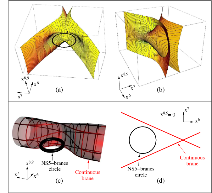
Figure 4: Semi-classical picture of the single-sheeted continuous brane. It is invariant under rotation in the plane $(x^{8},x^{9})$. The values of the parameters used to draw the brane are: $c=1.2$, $\theta_{0}=\frac{\pi}{8}$, $\psi_{0}-\omega_{0}=0$. The circle of NS5-branes is also shown. (a),(b): The single-sheeted continuous brane as seen from two different points of view (in Euclidean space). (c) A sketch of the single-sheeted continuous brane, taking into account the non-trivial metric in space-time. (d) The intersection of the single-sheeted continuous brane with the plane containing the circle of NS5-branes.

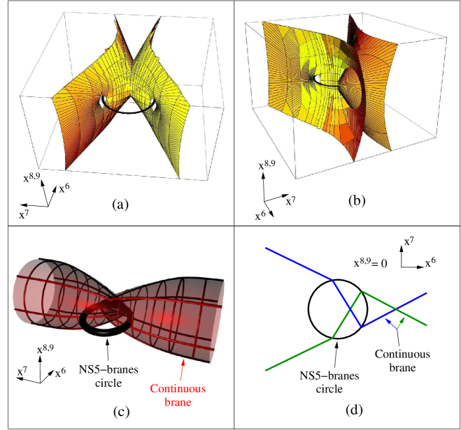
Figure 5: Semi-classical picture of the double-sheeted continuous brane. It is invariant under rotation in the plane $(x^{8},x^{9})$. The values of the parameters used to draw the brane are: $c=0.8$, $\theta_{0}=\frac{\pi}{8}$, $\psi_{0}-\omega_{0}=0$. The circle of NS5-branes is also shown. (a), (b): The double-sheeted continuous brane as seen from two different points of view (in Euclidean space). (c): A sketch of the double-sheeted continuous brane, taking into account the non-trivial metric in space-time. (d) The intersection of the double-sheeted continuous brane with the plane containing the circle of NS5-branes. The two sheets are drawn with different colors.

The parameter $\tilde{\omega}$ extends from zero to $2\pi$. The direction of the brane in the plane $(x^{6},x^{7})$ is given by the angle $\psi_{0}-\omega_{0}$, which is fixed by the combination of the brane parameters $\hat{n}-2\hat{m}$. The same combination appears in the condition of mutual supersymmetry for two branes (equation (71)). This means that mutually supersymmetric branes are parallel . The orthogonal combination $\hat{n}+2\hat{m}$ gives the value of a Wilson line on the brane. The shape of the brane is shown in figures 4 and 5. We observe that there are two physically different configurations for this brane, according to the value of the parameter $c$. For $c>1$, the brane does not intersect the circle of NS5-branes. It is composed of a single self-intersecting sheet. For $c<1$, the brane does intersect the circle of NS5-branes. It is composed of two distinct sheets. If the parameters $c$ and $\theta_{0}$ satisfy $1>c>\sin\theta_{0}$, the two sheets intersect each other, as shown in figure 5. On the other hand, if the parameters are such that $c<\sin\theta_{0}$, the two sheets do not intersect each other.

Notice that the continuous brane in the conformal field theory has positive parameters $\hat{J}$ and $\hat{j}$, which implies that the geometric parameters $c$ and $\theta_{0}$ satisfy: $c\geq\cos\frac{2\pi}{2k}\geq\sin\theta_{0}$. The conformal field theory description of continuous branes with parameter $c$ smaller than $\cos\frac{2\pi}{2k}$ is an interesting open problem. We will make this analysis more precise in section 5.2.

For the discrete branes, the parameter $c$ is always smaller than one and quantized (cf. equation (45)). The semi-classical description is otherwise identical.

D-branes in the presence of fluxes and the di-electric effect

We will now argue that the continuous brane can be thought of as a stack of D4-branes blown-up by the di-electric effect. We first discuss this effect in the asymptotic region, where the doubly scaled geometry (50) simplifies to $\mathbb{R}_{(r)}\times S^{3}_{(\theta,\phi,\psi)}$. The radius of the three-sphere is equal to $\sqrt{k\alpha^{\prime}}$. This is the geometry of the throat created by $k$ NS5-branes. In this region the geometry of the continuous brane (73) simplifies to:

$$\left\{\begin{array}[]{l}r\gg 1\\ \sin(\theta)\sin(\psi-\psi_{0})=\pm\sin(\theta_{0})\end{array}\right.$$ (74)

The second line defines two anti-podal two-spheres embedded in the three-sphere $(\theta,\phi,\psi)$. The radius of these two-spheres is equal to $\sqrt{k\alpha^{\prime}}\cos\theta_{0}$. We deduce that the geometry of the continuous brane far from the circle is $(S^{2}+S^{2})\times\mathbb{R}$, as drawn in figure 6 (a). So in the full NS5-brane background (46), the tube goes into and out of the throat (cf. figure 6 (b)).

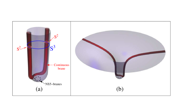
Figure 6: The shape of the continuous brane far from the NS5-branes. (a) In the doubly scaled geometry (50), the intersection of the continuous brane with the transverse three-sphere is given by two anti-podal two-spheres. (b) In the full NS5-brane background (46), the continuous brane has two legs getting out of the throat.

D-branes of low dimensional world-volume in the presence of fluxes tend to develop additional world-volume dimensions (see [38] for the case of RR fluxes and [39] for the case of NSNS fluxes). This is a di-electric effect. In particular in [39] it was shown that $n$ coincident D0-branes in the $SU(2)_{k}$ WZWN model tend to decay to a single spherical D2-brane. The radius of this brane is $\sqrt{k\alpha^{\prime}}\sin(\pi n/k)$ [31].

The same phenomenon arises in the NS5-brane background (50), since the NS5-branes source NSNS-flux on the three-sphere $S^{3}_{(\theta,\phi,\psi)}$. So even though the world-volume of the continuous brane (73) is seven-dimensional (three-dimensional in the transverse space $x^{6,7,8,9}$, and also extended in four flat directions), we can also think of this single extended D6-brane as a stack of $n$ coincident D4-branes. We identify the number $n$ of D4-branes via the radius of the two-spheres defined by equation (74):

$$n=2\hat{j}+1$$ (75)

The D-branes with one dimension in the transverse space $x^{6,7,8,9}$ and extremizing the DBI action in the NS5 background (46) are straight lines in the $x^{6,7,8,9}$ coordinates. When we minimize the tension as well as the length, the harmonic function drops out in the calculation. Since the brane (73) is invariant under rotation in the $(x^{8},x^{9})$ plane, we consider only D-branes that preserve that symmetry. They are straight lines in the $(x^{6},x^{7})$ plane, located at the origin of the $(x^{8},x^{9})$ plane. The direction of this line is given by the angular parameter $\psi_{0}-\omega_{0}$, and the coordinate distance to the origin is given by the parameter $c$ multiplied by $\rho_{0}$.

In fact, we are considering the bulk and brane system in a triple scaling limit, which consists of the usual double scaling limit in the bulk, and a third limit that scales the coordinate distance of the branes to the NS5-branes to zero, commensurate with the scaling down of the coordinate distance between the NS5-branes, such that the ratio (equal to the parameter $c$) is fixed.

We now understand that equations (73) describe the manifestation of the di-electric effect for D4-branes in the presence of a circle of NS5-branes. A stack of coincident D4-branes decays to a single D6-brane which shape is given by (73) (cf. figure 7). Far from the circle, the D6-brane has geometry $(S^{2}+S^{2})\times\mathbb{R}$ in the transverse space $x^{6,7,8,9}$. Close to the NS5-branes, the two-spheres are deformed by the repulsion between the NS5-branes and the D6-brane. We can understand the way the two-spheres are deformed as follow. Consider the two-sphere on one leg of the brane. The north pole of the sphere is pulled inwards as we get closer to the NS5-branes. It reaches the south pole and goes beyond as the distance to the NS5-branes increases again. We end up on the second leg with the second two-sphere. The two-sphere changes orientation in the process.

In more detail, consider for example the case where the D4-branes do not intersect the circle of NS5-branes ($c>1$). The $\mathbb{Z}_{2}$ symmetry $\psi\to-\psi+2\psi_{0}-2\omega_{0}$ has a fixed point at $\psi=\psi_{0}-\omega_{0}$: this is the point where the D4-branes are closest to the circle of NS5-branes. This particular angular direction also defines the locus of the self-intersection of the continuous brane (73). In terms of the coordinates $x^{6,7,8,9}$ defined in (48), this surface has equation:

$$\left\{\begin{array}[]{l}-\sin\psi_{0}x^{6}+\cos\psi_{0}x^{7}=0\\ \left(\cos\psi_{0}x^{6}+\sin\psi_{0}x^{7}-\frac{\rho_{0}}{2}\left(\frac{c}{\sin\theta_{0}}+\frac{\sin\theta_{0}}{c}\right)\right)^{2}+(x^{8})^{2}+(x^{9})^{2}=\rho_{0}^{2}\left(\frac{1}{4}\left(\frac{c}{\sin\theta_{0}}+\frac{\sin\theta_{0}}{c}\right)^{2}-1\right)\\ \cos\psi_{0}x^{6}+\sin\psi_{0}x^{7}\geq c\sin\theta_{0}\end{array}\right.$$ (76)

The first two lines describe a surface with topology of a two-sphere, while the third line removes a piece of this surface. Actually, the surface is double-sheeted and without boundary. Indeed, this surface describes the deformed two-sphere of the continuous brane at the point where the north pole meets the south pole and the sphere changes orientation (cf. figure 7).

When the stack of D4-branes intersects the circle, with parameters such that $1\geq c\geq\sin\theta_{0}$, the D6-brane has two sheets that intersect each other along the surface defined by the same equations (76). However this time the inequality is always satisfied, and we have a full two-sphere. If the parameters satisfy $c<\sin\theta_{0}$, the two sheets of the brane do not intersect each other anymore.

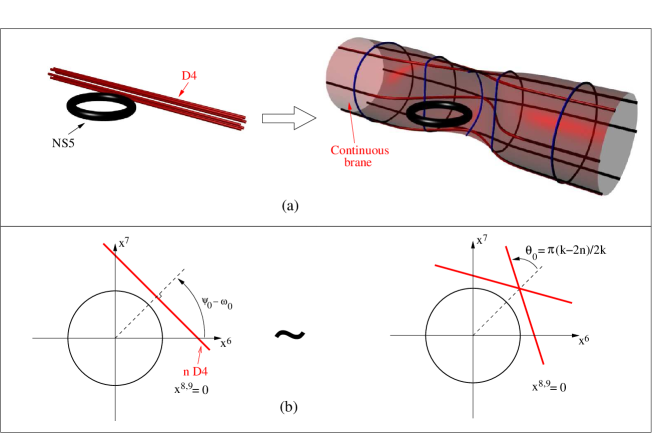
Figure 7: The di-electric effect for a stack of D4-branes in the presence of a circle of NS5-branes. (a) The coincident D4-branes are blown up to a single continuous brane. Far from the circle, the continuous brane has geometry $(S^{2}+S^{2})\times\mathbb{R}$ in the transverse space $x^{6,7,8,9}$. Close to the circle, the two-spheres are deformed by the repulsion between the D6-brane and the NS5-branes. (b) The intersection of the previous D-branes with the plane containing the NS5-branes. We indicate how the parameters defining the continuous brane and the straight D4-branes are related.

Identity branes

To obtain a semi-classical description of the identity branes, it is convenient to consider them in the background mirror to (52), where the trumpet is replaced by the cigar and the region near the tip is under geometric control. Building the identity branes in the conformal field theory mirror to (54), we can deduce the semi-classical description of the identity branes in the Neveu-Schwarz five-brane background (50) [5]. We can also use the following semi-classical description of the identity brane in the trumpet geometry (38):

$$r=0\ ;\ \psi-\psi_{\mathbb{I}}=0\$$ (77)

with the angular direction $\psi_{\mathbb{I}}$ defined in terms of the brane parameter $\hat{m}$ as:

$$\psi_{\mathbb{I}}=2\pi\frac{\hat{m}}{k}.$$ (78)

Then we perform a T-duality as in the previous case to get the semi-classical description of the identity branes in the NS5-brane background:

$$\left\{\begin{array}[]{l}r=0\\ \sin(\theta)\sin\left(\psi-\psi_{\mathbb{I}}+\omega_{0}\right)=\sin(\theta_{0})\end{array}\right.$$ (79)

The parameters $\theta_{0}$ and $\omega_{0}$ are defined in terms of the brane parameter $\hat{j}$ and $\hat{n}$ in (60). The parameter $\hat{j}$ fixes the length of the brane. These branes are straight lines in the $(x^{6},x^{7})$ plane, starting and ending on the circle of NS5-branes. As for the continuous branes, the combination of the brane parameters $\hat{n}-2\hat{m}$ gives the angular orientation of the brane.

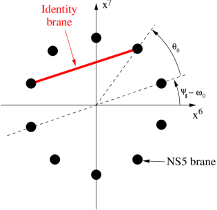
Figure 8: Semi-classical description of an identity brane, stretching between NS5-branes.

In the minimal model, the choice of parameters $\hat{j}$, $\hat{n}$, $\hat{s}_{2}$ is constrained by the selection rule (namely: $2\hat{j}+\hat{n}+\hat{s}_{2}$ is zero modulo two). As a consequence, the length of an identity brane is related to its orientation. Note that even though the NS5-branes have been spread on the circle, their position is still coded in the worldsheet instantons. We make the minimal assumption that the identity branes are suspended between NS5-branes. Since the identity branes are defined only for integer values of the parameter $\hat{m}$, this assumption is consistent with the selection rule in the minimal model. The semi-classical description of the identity branes gives a way to recover the positions of the NS5-branes on the circle.

5.2 D-branes cut in two pieces

Consider a continuous brane (61). In order to obtain a semi-classical picture of the operation we performed in the exact boundary conformal field theory, we study what happens when the brane parameter $\hat{J}$ goes to one half (i.e. the imaginary part of $\hat{J}$ goes to zero), keeping all the other brane parameters fixed. The geometric parameter $c$ goes down to one as the brane parameter $\hat{J}$ goes to one-half. When the geometric parameter $c$ is equal to one, the continuous brane touches the circle and is on the verge of being cut into two intersecting sheets.

Let’s make this point more precise. First notice that the surface (73) is symmetric under the reflection $\psi-\psi_{0}+\omega_{0}\to-(\psi-\psi_{0}+\omega_{0})$ (together with $\tilde{\omega}\to\pi-\tilde{\omega}$). Figures 4 and 5 suggest that when the brane is cut, the two sheets are exchanged by this symmetry. We would like to know whether there exists a smooth path $\gamma$ on the brane connecting two symmetric points, of respective angular coordinate $\psi_{1}$ and $-\psi_{1}+2\psi_{0}-2\omega_{0}$. The value of the parameter $\tilde{\omega}$ for these points is noted respectively $\tilde{\omega}_{1}$ and $\pi-\tilde{\omega}_{1}$. Along the path $\gamma$, the angular coordinate $\psi$ goes smoothly from $\psi_{1}$ to $-\psi_{1}+2\psi_{0}-2\omega_{0}$, and the parameter $\tilde{\omega}$ goes smoothly from $\tilde{\omega}_{1}$ to $\pi-\tilde{\omega}_{1}$. Notice that the parameter $\tilde{\omega}$ has to stay within the range $\theta_{0}\leq\tilde{\omega}\leq\pi-\theta_{0}$ for the equations (73) to have a solution. For the same reason the sum $\psi-\psi_{0}+\omega_{0}+\tilde{\omega}$ must be positive and smaller than $\pi$. We deduce that along the path $\gamma$, the sum $\psi-\psi_{0}+\omega_{0}+\tilde{\omega}$ goes smoothly from $\psi_{1}-\psi_{0}+\omega_{0}+\tilde{\omega}_{1}$ to $\pi-(\psi_{1}-\psi_{0}+\omega_{0}+\tilde{\omega}_{1})$, necessarily crossing the value $\psi-\psi_{0}+\omega_{0}+\tilde{\omega}=\frac{\pi}{2}$. But this is possible if and only if the brane parameter $c$ is greater or equal to one. Indeed, if $c<1$, the first equation in (73) does not have solutions for $\psi-\psi_{0}+\omega_{0}+\tilde{\omega}=\frac{\pi}{2}$. The conclusion is that the path $\gamma$ exists for $c\geq 1$. In that case, the two points are smoothly connected and the brane is single-sheeted. If $c<1$, there is no smooth path between two symmetric points, and the brane is made of two distinct sheets. If $1>c>\sin\theta_{0}$, the two sheets of the brane intersect and one can find a path between two symmetric points. However the parameter $\tilde{\omega}$ will not vary continuously along such a path, indicating that we pass from one sheet onto the other.

We argued in the previous section that the continuous D6-brane can be interpreted as a stack of D4-branes. The cutting of the D6-brane in two sheets can also be understood in terms of the D4-branes. As the D4-branes hit the NS5-circle, they are cut in two semi-infinite pieces (see figure 9).

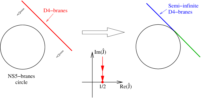
Figure 9: A stack of D4-branes approaches a circle of NS5-branes, as the brane parameter $\hat{J}$ goes to one-half. For $\hat{J}=\frac{1}{2}$ the D4-branes are cut in two pieces.

The brane addition relation (21) is valid precisely at the point where the D6-brane is cut in two pieces. That implies that the continuous brane with parameter $\hat{J}=\frac{1}{2}$ (and $\hat{m}$ half-integer) is the sum of two discrete branes. The picture obtained in the conformal field theory fits nicely with the semi-classical analysis.

5.3 D-branes cut in three pieces

Now we want to study the continuous brane when it gets inside the circle of NS5-branes, that is for values of the parameter $c$ smaller than one. Consider a continuous brane (61) with parameter $\hat{m}$ integer (and any value for the other parameters). We study what happens when the parameter $\hat{J}$ goes to zero, keeping all the other parameters fixed. That mirrors what we did in section 2.5, while computing the overlap of continuous branes in Liouville theory. The addition relation (20) implies that an identity brane (63) appears when the continuous brane parameter $\hat{J}$ is equal to zero. The identity brane created has the same parameters as the continuous brane. We will now understand the appearance of this identity brane from the semi-classical analysis of the continuous branes.

Let’s first consider the simpler case in which the continuous brane parameter $\hat{j}$ is zero. In this situation, the continuous D6-brane represents one single D4-brane. Now we observe that at the special value of the brane parameter $\hat{J}=0$, the geometric parameter $c$ is equal to $\cos(\frac{2\pi}{2k})$: we are considering the situation where the D4-brane hits a pair of neighboring NS5-branes (cf. figure 10). The compact part of the D4-brane that stretches between the NS5-branes matches precisely the semi-classical description (79) of the identity brane on the right-hand side of equation (20). We conclude that in this case the brane addition relation (20) captures the fact that the D-brane hitting two separated NS5-branes consists of three pieces.

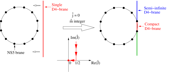
Figure 10: A particular case: a single D4-brane approaches a circle of NS5-branes, as the brane parameter $\hat{J}$ goes to zero (the parameter $\hat{m}$ is integer). For $\hat{J}=0$ the D4-brane is cut in three pieces. Massless open strings live on the compact piece.

Next, let’s consider the generic case where the brane parameter $\hat{j}$ is non-zero. The identity brane that appears does not stretch between neighboring NS5-branes. To understand the appearance of such a compact brane, we have to take into account the blowing up of the stack of D4-branes by the di-electric effect. In figure 11 we draw the intersection of the continuous brane (73) with the plane containing the circle of NS5-branes. We observe that at the special value of the brane parameter $\hat{J}=0$, the intersection of the continuous brane with the interior of the circle of NS5-branes matches (up to corrections of order $\frac{1}{k}$) the semi-classical description (79) of the identity brane that is generated. We are still describing D-branes that are cut into three pieces when hitting two separated NS5-branes. But the way the D-branes are cut is less intuitive, because they are blown up by the di-electric effect.

The computation of section 2.5 tells us that when the parameter $\hat{J}$ is equal to $\frac{1}{4}$, new massive states appear on the continuous brane. They are bound states on the world-volume on the brane. The mass of these states goes down as the parameter $\hat{J}$ goes to zero. At the special value of the parameter $\hat{J}=0$, some of these localized states become massless. The new massless modes live on the identity brane of the addition relation (20). So the appearance of poles in the densities of states studied in section 2.5 corresponds to the gradual creation of a new brane in space-time.

Another way to see this is to look at the $D0$-charge on the continuous $D2$-brane in the cigar. The $D0$-charge is defined as: $\frac{2}{2\pi}\int F=\frac{2k}{2\pi}\arcsin c$. The additional factor of two comes from the fact that the brane is double-sheeted. As the parameter $c$ goes from 1 to $\cos\frac{2\pi}{2k}$, the $D0$-charge changes by one unit. In our context, this corresponds to the creation of one unit of D4-brane charge.

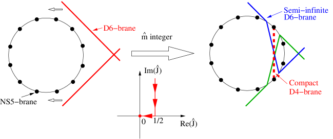
Figure 11: The generic case: a continuous brane approaches a circle of NS5-branes, as the brane parameter $\hat{J}$ goes to zero (the parameter $\hat{m}$ is integer). For $\hat{J}=0$ an identity brane appears, sketched by a dotted line. Massless open strings live on this compact brane.

The fact that the addition relation (20) is only valid for integer values of the brane parameter $\hat{m}$ is consistent with the position of the NS5-branes on the circle, and thus with the selection rule in the minimal model.

We repeat that the movement of the continuous brane as the parameter $\hat{J}$ changes is infinitesimal when measured in the asymptotic flat space metric (due to the triple scaling). Indeed the geometry of the continuous brane far from the circle (given by equations (74)) does not depend on the parameter $\hat{J}$.

It would be interesting to study what happens when the continuous brane gets even closer to the center of the NS5-branes circle. However making the analytic continuation of the continuous brane parameter $\hat{J}$ to negative values is not the right way to proceed, since it induces the appearance of non-unitary characters of the $N=2$ superconformal algebra. An alternative could be to introduce a non-factorized brane as the continuation of the continuous brane beyond $\hat{J}=0$.

6 Four-dimensional gauge theory in the depths of the throat

The discussion of the previous section is valid independent of the boundary conditions we choose for the flat space directions (provided we have at least two directions with Dirichlet boundary conditions). In this section we focus on D4-branes, extended in the $x^{0,1,2,3,6}$ directions and localized in the other directions, as well as mutually supersymmetric D6-branes. We perform an analysis of the low-energy excitations on these branes, and a preliminary analysis of their interactions.

6.1 Energy scales

First we specify the energy scales on which we will focus. There are two fixed energy scales in the problem, namely the string scale $M_{s}=1/\sqrt{\alpha^{\prime}}$ and the curvature scale $M_{gap}=1/\sqrt{k\alpha^{\prime}}$. At the string scale oscillation modes become important. The curvature scale gives the order of the mass gap due to the linear dilaton, as well as the Kaluza-Klein mass gap due to compactification of some of the transverse directions. The low energy scales we focus on are energies far below both the string scale and the curvature scale.

6.2 Localized gauge theory on the non-compact brane

Let’s consider the theory living on a continuous brane of parameter $\hat{J}$. In the throat, due to the presence of the linear dilaton, the theory on a generic continuous brane is gapped, and at energies below $M_{gap}$ we have a theory with no excitations at all. Operationally, if $\hat{J}$ has an imaginary part, or we have real $\hat{J}$ in the range $1/4<\hat{J}\leq 1/2$ , the self-overlap of the continuous brane is given in equation (69) and all states are in massive representations. The theory at low energy is trivial in this case.

When we bring down the brane parameter into the range $0<\hat{J}<1/4$, the self-overlap of the continuous brane is given in equation (70). All the states are still in massive representations, but we notice that a state localizes and its mass drops below the mass gap $M_{gap}$. By tuning $\hat{J}$ to be close to $\hat{J}=0$, we can make the mass parametrically small compared to $M_{gap}$. At energies below that mass, we still have a trivial theory. We may get an interesting theory at energies squared between $2\hat{J}(1-2\hat{J})M_{gap}^{2}$ and $M_{gap}^{2}/4$.

At these energy scales, the theory is localized in the transverse space and is effectively four-dimensional. It has eight supercharges. Via the annulus amplitude we identify the excitations of the theory and they fill out a single massive gauge multiplet of four-dimensional ${\cal N}=2$ supersymmetry. We find a real massive vector, four Majorana spinors and five scalars. If we denote the normalizable bound state in the full theory (at $j=0=n$) by:

$$|k_{\mu=0,1,2,3},0,[\hat{J}]\rangle$$ (80)

then the excitations filling out the massive gauge multiplet are:

$$\psi^{2,3}_{-1/2}|k_{\mu},0,[\hat{J}]\rangle$$

$$\psi^{4,5}_{-1/2}|k_{\mu},0,[\hat{J}]\rangle$$

$$G_{-1/2}^{\pm,nc}|k_{\mu},0,[\hat{J}]\rangle$$

$$Sp_{\mp 1}G_{-1/2}^{\pm,nc}|k_{i},0,[\hat{J}]\rangle.$$ (81)

We have used the superscript $nc$ to denote an operator acting on the non-compact $N=2$ Liouville theory only and the notation $Sp_{\mp 1}$ indicates a spectral flow by $\mp 1$ units in both the minimal model and the non-compact model (at total central charge $c=6$). For instance, starting from the state $G_{-1/2}^{+,nc}|k_{\mu},0,[\hat{J}]\rangle$ we can generate another state of the same conformal dimension by spectrally flowing by minus one unit. The state we obtain is anti-chiral in the minimal model, with R-charge $-1+2/k$. It has R-charge $-2/k$ in the non-compact model for a total R-charge of $-1$. We refer to appendix B for an explicit analysis of how these states are coded in the annulus partition function in the particular case of $k=3$ NS5-branes.

The transverse polarizations of the massive vector are given by the first two states, while the other states give the longitudinal polarization as well as five scalar fields. We can figure out which scalar plays the role of the longitudinal polarization of the vector by the following reasoning. In an old covariant approach to the determination of the spectrum, we have a null state in the Hilbert space which corresponds to $G_{-1/2}^{N=1}|k_{\mu},0,[\hat{J}]\rangle$. It is a null state since $G^{N=1}$ is the supercurrent corresponding to the gauging of $N=1$ supergravity on the world-sheet. Explicitly, we have that this null state is:

$$k_{\mu}\psi^{\mu}_{-1/2}+G^{N=1,nc}_{-1/2}|k_{\mu},0,[\hat{J}]\rangle,$$ (82)

where we used the fact that the supercurrent annihilates the vacuum in the Dirichlet and the minimal model factors. Thus in the light-cone gauge where we broke Lorentz invariance and chose to fix the gauge symmetry by gauging away the light-cone excitations, we identify the scalar

$$G^{N=1,nc}_{-1/2}|k_{\mu},0,[\hat{J}]\rangle$$ (83)

as the longitudinal component of the massive vector field. The other five scalars complete the massive ${\cal N}=2$ vector multiplet.

When we proceed to consider a brane with parameter $\hat{J}=0$, we find that the massive vector multiplet splits into a massless vector multiplet and a massless hyper multiplet. By the previous reasoning, and the fact that $|k_{\mu},0,[0]\rangle$ is annihilated by both $G^{\pm,nc}_{-1/2}$, we find that the longitudinal polarization of the vector is now null (as it must be for a massless vector). There is then only one possible set of multiplets of the supersymmetry algebra corresponding to the vector and the six scalars, namely a massless vector and hyper multiplet. Explicitly, the massless vector multiplet has bosonic degrees of freedom:

$$\psi^{2,3}_{-1/2}|k_{\mu},0,[0]\rangle$$

$$\psi^{4,5}_{-1/2}|k_{\mu},0,[0]\rangle$$ (84)

and the massless hyper multiplet has four bosonic scalar degrees of freedom:

$$|k_{\mu},0,\pm 1/2\rangle$$

$$Sp_{\mp 1}|k_{\mu},0,\pm 1/2\rangle.$$ (85)

We indicated the discrete representation chiral and anti-chiral ground states by $|0,\pm 1/2\rangle$. Alternatively, at $\hat{J}=0$ we can interpret the excitations as coming from various overlaps of terms in the brane addition relation (20). The four bosonic degrees of freedom in the ${\cal N}=2$ vector multiplet arise from the self overlap of the identity brane on the right-hand side of the addition relation (20). The other massless states come from the overlap of the identity brane with the discrete branes. This overlap contains the discrete characters of (12). In the character $Ch_{d}(J=\frac{k}{2},r=0)$ we find one chiral primary state with $U(1)$ R-charge $Q=1$, and the spectral-flowed anti-chiral primary with $Q=-\frac{k}{2}$. These states combine with chiral and anti-chiral primary from the minimal model and the flat direction to give massless modes (with $Q=\pm 1$). In the second discrete character $Ch_{d}(J=1,r=-1)$ we find one anti-chiral primary state with $Q=-1$, and the spectral-flowed chiral primary with $Q=\frac{k}{2}$. Notice that from the right-hand side of (20), we expect eight massless bosonic states from the overlap of the identity brane with the two discrete branes. However half of them are canceled by the self overlap of the discrete branes, as shown in appendix A.

Interactions

In the spectrum of excitations, we witnessed a reverse Higgs mechanism consistent with ${\cal N}=2$ supersymmetry in four dimensions. When we survey what the relevant Higgs mechanism can be, consistent with ${\cal N}=2$ supersymmetry in four dimensions (see [41]), we find only one candidate. A real massive vector multiplet arises when we add a Fayet-Iliopoulos D-term to a $U(1)$ theory with a charged hyper multiplet. The vector multiplet and the hyper multiplet acquire equal masses (proportional to the charge times the FI-parameter). Indeed, we did find that as we change $\hat{J}$, the vector and hyper multiplet acquire the same mass.

To nail down this picture we need to analyze the interactions between open string states to verify the presence of the necessary cubic and quartic interaction terms. That may be doable on the basis of the results of [42] that map boundary $n$-point functions in $H_{3}^{+}$ into an in principle solved problem in boundary bosonic Liouville theory. One can apply this reduction to boundary $N=2$ Liouville theory and thus determine the open string interaction terms. We will not attempt to perform this calculation here. It would be interesting to do it, and in particular to prove explicitly that at non-zero $\hat{J}$ the hyper multiplet is indeed charged.

Without the necessary study of the interaction terms we can make one more observation that is consistent with the Higgs mechanism advocated above, which is the breaking of the (accidental) R-symmetry (at low energy). When the brane parameter $\hat{J}$ is zero, the Hilbert space of open strings splits into identity and discrete sectors. The scalars in the hyper multiplet are at the lowest level available in their sector, and there are no null states at the lowest level. Moreover, the action of the supersymmetry generators pairs up the scalars into doublets of the $U(2)_{R}$ symmetry of the theory. Each scalar pairs up with its spectral flowed counterpart. On the other hand, when the brane parameter is non-zero, the low-energy symmetry that exchanged the two scalars does not commute anymore with the BRST operator (as can clearly be seen by the existence of the null state that we mentioned above). The $U(2)_{R}$ symmetry gets broken to a $U(1)_{R}$ that does not act on the component of the complex doublet in the hyper that acquires a vacuum expectation value.

Finally, we note that at $\hat{J}=0=\hat{m}$ we have that a marginal deformation of type F on the world-sheet (i.e. the holomorphic square root of the bulk Liouville potential) becomes precisely one of the normalizable massless scalars in the hyper multiplet. The fact that we add such a term to the world-sheet action in order to turn up the value of $\hat{J}$ is consistent with the fact that the corresponding field acquires a vacuum expectation value. More precisely, we have the relations [11]:

$$\mu_{A} = \sqrt{\frac{2k\mu}{\pi}}\sin\pi(-\hat{J}-\hat{m})$$

$$\bar{\mu}_{A} = \sqrt{\frac{2k\mu}{\pi}}\sin\pi(-\hat{J}+\hat{m})$$ (86)

for the coefficients $\mu_{A}$ and $\bar{\mu}_{A}$ of the F-terms on the boundary of the world-sheet which are holomorphic square roots of the bulk Liouville potential. In a covariant formulation, and for a zero momentum $k_{\mu}=0$ ground state, we note that the combination $G^{N=1,nc}|0,0,[\hat{J}]\rangle$ is pure gauge. We conclude that for very small non-zero $\hat{J}$ and $\hat{m}$, the null deformation, which will not change the spectrum on the non-compact brane will correspond to the deformation $\mu_{A}=-\bar{\mu}_{A}$ (since the brane parameter $\hat{m}$ does not change the spectrum). Therefore the $\hat{J}$ deformation near $\hat{J}=0$ corresponds to the deformation $\mu_{A}=+\bar{\mu}_{A}$. Thus, infinitesimally near $\hat{J}=0=\hat{m}$, we have a complex scalar field which has one component which becomes the longitudinal component of the massive vector boson, and an orthogonal component which acquires a vacuum expectation value.

Remark

An interesting open problem is to attempt to give a mass to the hyper multiplet while keeping the vector multiplet massless. A naive attempt to separate the identity brane from the rest of the $\hat{J}=0$ brane would fail because the remainder does not pass the Cardy check. Another way to put this is to note that one would generate two massive hyper multiplets, and minus one massless hyper multiplet.

6.3 The gauge theory on the compact branes

We turn to the gauge theory on the compact identity branes. We will be brief since the theory has been analyzed before. The identity branes are stretched between two NS5-branes. The effective gauge theory below the curvature scale $M_{gap}$ is four dimensional. The low-energy theory contains one massless vector multiplet of ${\cal N}=2$ supersymmetry in four dimensions, and gives rise to a pure $U(N)$ super-Yang-Mills theory for $N$ compact branes. They have been discussed as exact boundary states in [7][5][23].

6.4 Combining branes

If we consider simultaneously non-compact and compact branes, we must consider whether they are mutually supersymmetric. Once we fix the parameters $\hat{m}$ and $\hat{n}$ of the identity brane (which fix its orientation) then we must fix the non-compact brane orientation such that the brane is parallel. We then preserve eight supercharges again. At energy scales below the mass gap but above the energy $\hat{J}M_{gap}$, we have a massive vector multiplet of mass squared $-2\hat{J}(2\hat{J}-1)/k\alpha^{\prime}$, a complex massive vector with a mass squared $-\hat{J}(\hat{J}-1)/k\alpha^{\prime}$ as well as the massless vector multiplet on the identity brane. The real massive vector multiplet and the massless vector multiplet on the identity brane have been discussed before.

The complex massive vector multiplet embodies a Higss mechanism of the second type [41] in which one vector multiplet eats a scalar of another vector multiplet and vice versa. In more modern language, we go to a Coulomb branch of an ${\cal N}=2$ gauge theory. Again, to render the ${\cal N}=2$ gauge theory interactions manifest, we would need to analyze in detail the open string interactions.

7 Two NS5-branes

The case of two NS5-branes is an interesting special case. When we spread two branes on a circle, they are in fact spread on a line (which we will take to be the $x^{6}$ direction). We therefore preserve a larger symmetry group in this case, which includes an $SO(3)_{789}$ isometry group (enlarged to $O(3)$ due to the $Z_{2}$ operation interchanging the two NS5-branes). We will use this extension of the symmetry group to make an interesting consistency check on our claims in previous sections. In the exact conformal field theory at $k=2$, the minimal model becomes trivial. The bulk theory and its symmetries were thoroughly analyzed in [43]. We recall that at level $2$ we can fermionize the asymptotic angular variable $\theta$ in Liouville theory by the equivalence $e^{\pm i\theta}=\frac{1}{\sqrt{2}}(\psi_{1}\pm i\psi_{2})$. This allows us to define the $SU(2)_{2}$ affine currents:

$$J_{i} = (\psi_{\rho}\psi_{i}-\frac{1}{2}\epsilon_{ijk}\psi_{j}\psi_{k})e^{-\rho},$$ (87)

where $\psi_{3}$ is the fermionic partner of the angular variable $\theta$ and $\psi_{\rho}$ is the superpartner of the asymptotic radial direction $\rho$. From the detailed arguments in [43], one concludes that the bulk Liouville deformation can be chosen such as to preserve a diagonal $SU(2)_{2}$ current algebra. It is this local symmetry algebra on the world-sheet that generates the $SO(3)_{789}$ isometry group in space-time (in the doubly scaled regime).

We wish to add non-compact branes to this configuration. In doing so we observe that there is a single non-compact D4-brane that we can add to the asymptotically flat configuration which will preserve the $SO(3)_{789}$ isometry group. It is the non-compact D4-brane that stretches along the line separating the $NS5$-branes (namely the $x^{6}$ direction) and coinciding with the NS5-branes in the transverse space $x^{7,8,9}$. From the arguments in the previous section, we expect that that brane should correspond to the non-compact brane at $\hat{J}=0=\hat{m}$ after descending down the throat.

We can test this directly in the full exact conformal field theory, using the symmetry algebra above. From the results of [43] and [11] it is clear that the three currents evaluated on the boundary correspond precisely to the two marginal F-term deformations and the marginal D-term deformation of boundary $N=2$ Liouville theory. Thus, the boundary deformations form a triplet of $SO(3)_{789}$. Consequently, when any of these boundary deformations is turned on, we break $SO(3)_{789}$. We already saw that the F-term boundary deformations are generically zero at $\hat{J}=0=\hat{m}$ (see equation (6)). So, to check whether $SO(3)_{789}$ is preserved we need to check whether also the third deformation parameter is zero. It has the value [11]:

$$\tilde{\mu}_{A} = -\nu^{\frac{1}{2}}\frac{\Gamma(-1/k)}{2\pi k}\cos\frac{\pi}{k}(2\hat{J}-1).$$ (88)

We observe that precisely at the value $k=2$, and $\hat{J}=0$ the third boundary deformation parameter $\tilde{\mu}_{A}$ is zero as well. In summary, we used a particularly symmetric set-up to provide a powerful consistency check on our identification of the brane $\hat{J}=0=\hat{m}$ as the brane that splits on two NS5-branes.

8 Conclusions

In this paper, we have demonstrated character identities for the $N=2$ superconformal algebra, which lead to the introduction of addition relations for boundary states. We then showed the appearance of localized bound states in the spectrum of non-compact branes, both via an analytic and an algebraic approach.

These interesting properties of non-rational $N=2$ Liouville theory find applications in string theory. We analyzed one application in detail, for branes in the background of NS5-branes spread on a circle. There we showed that the addition relations are reflected in semi-classical properties of D-branes with three directions transverse to the NS5-branes. We also gave an exact conformal field theory analysis of the spectrum on these branes, and showed the appearance of interesting open string bound states localized deep down the throat of NS5-branes (in a triple scaling limit). We performed a preliminary analysis of the gauge theory interactions that govern these bound states at low energy.

There remain many interesting open questions related to our work. We mention only a few interesting routes. The four-dimensional gauge theory we identified deserves more investigation. The computation of the interactions of the bound states at low energy would be a useful enterprise. It would also be interesting to apply what we have learned about $N=2$ Liouville theory to configurations that preserve only four supercharges. Another direction would be the construction of boundary states that do not factorize in terms of the coset conformal field theories, and find their interpretation in terms of D-branes in NS5-brane backgrounds. This is presumably related to the problem of giving a mass to the hyper multiplet living on the non-compact brane, while keeping the vector multiplet massless. We hope to return to some of these open problems in the near future.

Appendix A Full Cardy states in $N=2$ Liouville

In this appendix we review the detailed construction of the full Cardy states in $N=2$ Liouville theory [7], including the couplings to the discrete Ishibashi states. We also compute the annulus amplitudes for arbitrary discrete branes. We show that discrete characters appear in the open string channel with multiplicities that are generically not positive integers.

We carefully normalize our amplitudes and one-point functions as follows. We fix the normalization of the continuous Ishibashi states such that their overlap is $\delta(P-P^{\prime})$. Our convention for the normalization of the closed string momentum (and therefore of the $\delta$-function) is such that $J=1/2+iP$ determines the Casimir of an $SL(2,\mathbb{R})$ representation. We take the $\delta$-function to be the $\delta$-function on the real half-line, namely $\int_{0}^{\infty}dP\delta(P-P^{\prime})f(P)=f(P^{\prime})$ for a function $f$ defined on the positive half-line. Also, we integrate over Ishibashi states with positive momentum $P$ only. That fixes the normalization of the one-point functions. In the closed string channel, we will sum over all integer momenta $2m$ (modulo $2k$).

The continuous and discrete Ishibashi states are defined as:

$$e^{-\pi\frac{c}{3}\frac{z^{2}}{T}}{}_{c}\langle\langle P,m|\mathrm{prop}|P^{\prime},m^{\prime}\rangle\rangle_{c}=\delta(P-P^{\prime})\delta_{m,m^{\prime}}Ch_{c}^{closed}(P,m;iT,z)$$ (89)

$$e^{-\pi\frac{c}{3}\frac{z^{2}}{T}}{}_{d}\langle\langle J,r|\mathrm{prop}|J^{\prime},r^{\prime}\rangle\rangle_{d}=\delta_{J,J^{\prime}}\delta_{r,r^{\prime}}Ch_{d}^{closed}(J,m;iT,z)$$ (90)

$$e^{-\pi\frac{c}{3}\frac{z^{2}}{T}}{}_{c}\langle\langle P,m|\mathrm{prop}|J,r\rangle\rangle_{d}=0$$ (91)

The closed string propagator is:

$$\mathrm{prop}=e^{\pi\frac{c}{3}\frac{z^{2}}{T}e^{-\pi TH^{(c)}}}e^{i\pi z(J_{0}+\bar{J}_{0})}$$ (92)

where $H^{(c)},J_{0},\bar{J}_{0}$ represent the cylinder Hamiltonian and the $U(1)R$ charge operators.

In section 2.3 we introduced the continuous, discrete and identity branes in $N=2$ Liouville theory, and gave their one-point functions to the continuous operators. The couplings to the discrete operators are:

$$\psi^{c}_{\hat{P},\hat{m}}(J,r)=0$$ (93)

$$\psi^{d}_{\hat{J},\hat{r}}(J,r)=\frac{i}{\sqrt{2k}}\frac{1}{\sqrt{\sin(\frac{\pi(2J-1)}{k})}}e^{-4\pi i\frac{(\hat{J}+\hat{r})(J+r)-(\hat{J}-1/2)(J-1/2)}{k}}$$ (94)

$$\psi^{\mathbb{I}}_{\hat{m}}(J,r)=\sqrt{\frac{2}{k}}\sqrt{\sin\left(\frac{\pi(2J-1)}{k}\right)}e^{-4\pi i\frac{2\hat{m}(J+r)}{2k}}.$$ (95)

Modular transformations

In the computation of annulus amplitudes, modular S-transformations are needed to switch between the closed string channel and the open string channel. We give below the relevant modular transformations for the characters of the extended $N=2$ superconformal algebra.

$$Ch_{c}^{closed}(P,m;-\frac{1}{\tau},\frac{z}{\tau})=e^{i\pi\frac{c}{3}\frac{z^{2}}{\tau}}\frac{2}{k}\sum_{2m^{\prime}=0}^{2k-1}e^{-4\pi i\frac{mm^{\prime}}{k}}\int dP^{\prime}\cos\left(4\pi\frac{PP^{\prime}}{k}\right)Ch_{c}^{open}(P^{\prime},m^{\prime};\tau,z)$$ (96)

$$Ch_{d}^{closed}(J,r;-\frac{1}{\tau},\frac{z}{\tau})=e^{i\pi\hat{c}\frac{z^{2}}{\tau}}\times$$

$$\left[\frac{1}{k}\sum_{2m^{\prime}=0}^{2k-1}e^{-4\pi i\frac{(J+r)m^{\prime}}{k}}\int dP^{\prime}\frac{\cosh(2\pi P^{\prime}\frac{k+1-2J}{k})+e^{i\pi 2m^{\prime}}\cosh(2\pi P^{\prime}\frac{2J-1}{k})}{2|\cosh(\pi(P^{\prime}+im^{\prime}))|^{2}}Ch_{c}^{open}(P^{\prime},m^{\prime};\tau,z)\right.$$

$$+\frac{i}{k}\sum_{r^{\prime}=0}^{k-1}\sum_{2J^{\prime}=2}^{k}e^{-4\pi i\frac{(J+r)(J^{\prime}+r^{\prime})-(J-\frac{1}{2})(J^{\prime}-\frac{1}{2})}{k}}Ch_{d}^{open}(J^{\prime},r^{\prime};\tau,z)$$

$$\left.+\frac{i}{2k}\sum_{r^{\prime}=0}^{k-1}e^{-4\pi i\frac{(J+r)(r^{\prime}+\frac{1}{2})}{k}}\left(Ch_{d}^{open}\left(\frac{1}{2},r^{\prime};\tau,z\right)+Ch_{d}^{open}\left(\frac{k+1}{2},r^{\prime};\tau,z\right)\right)\right]$$ (97)

$$Ch_{\mathbb{I}}^{closed}(m;-\frac{1}{\tau},\frac{z}{\tau}) = e^{i\pi\hat{c}\frac{z^{2}}{\tau}}\times$$ (98)

$$\left[\frac{1}{k}\sum_{2m^{\prime}=0}^{2k-1}e^{-4\pi i\frac{mm^{\prime}}{k}}\int dP^{\prime}\frac{\sinh(2\pi\frac{P^{\prime}}{k})\sinh(2\pi P^{\prime})}{|\cosh(\pi(P^{\prime}+im^{\prime}))|^{2}}Ch_{c}^{open}(P^{\prime},m^{\prime};\tau,z)\right.$$

$$+\left.\frac{2}{k}\sum_{r^{\prime}=0}^{k-1}\sum_{2J^{\prime}=2}^{k}\sin(\frac{\pi(2J^{\prime}-1)}{k})e^{-4\pi i\frac{(m(J^{\prime}+r^{\prime})}{k}}Ch_{d}^{open}(J^{\prime},r^{\prime};\tau,z)\right]$$

In the bulk of the paper, and in the following computations, we leave the argument $\tau,z$ of the characters implicit but indicate whether we consider the closed or the open string channel.

Annulus amplitudes

We compute the annulus amplitude for open strings stretching between two branes, taking into account the coupling to discrete operators.

• Identity / any

  $${}_{\mathbb{I}}\langle\hat{m}^{\prime}|\mathrm{prop}|\hat{m}\rangle_{\mathbb{I}}=Ch_{\mathbb{I}}^{open}(\hat{m}-\hat{m}^{\prime})$$ (99)

  $${}_{\mathbb{I}}\langle\hat{m}^{\prime}|\mathrm{prop}|\hat{P},\hat{m}\rangle_{c}=Ch_{c}^{open}(\hat{P},\hat{m}-\hat{m}^{\prime})$$ (100)

  $${}_{\mathbb{I}}\langle\hat{m}^{\prime}|\mathrm{prop}|\hat{J},\hat{r}\rangle_{d}=Ch_{d}^{open}(\hat{J},\hat{r}-\hat{m}^{\prime})$$ (101)

• Continuous / continuous

  This overlap is computed in detail in section 2.5. The result is given by equations (• ‣ 2.5) and (36).

• Continuous / discrete

  $${}_{c}\langle\hat{P}_{1},\hat{m}_{1}|\mathrm{prop}|\hat{J}_{2}\hat{,}r_{2}\rangle_{d}=\int_{0}^{\infty}dP\left[\rho_{1}^{c-d}(P|\hat{P}_{1},\hat{J}_{2})Ch_{c}^{open}(P,\hat{J}_{2}+\hat{r}_{2}-\hat{m}1)\right.$$

  $$\left.+\rho_{2}^{c-d}(P|\hat{P}_{1},\hat{J}_{2})Ch_{c}^{open}(P,\hat{J}_{2}+\hat{r}_{2}-k-\hat{m}1)\right]$$ (102)

  with

  $$\rho_{1}^{c-d}(P|\hat{P}_{1},\hat{J}_{2})=\frac{2}{k}\int_{0}^{\infty}dP^{\prime}\frac{\cos(4\pi\frac{PP^{\prime}}{k})}{\sinh(2\pi\frac{P^{\prime}}{k})\sinh(2\pi P^{\prime})}\sum_{\epsilon=\pm 1}\cosh\left(2\pi P^{\prime}\left(1+\frac{1-2\hat{J}_{2}}{k}+i\epsilon\frac{2\hat{P}_{1}}{k}\right)\right)$$ (103)

  $$\rho_{2}^{c-d}(P|\hat{P}_{1},\hat{J}_{2})=\frac{2}{k}\int_{0}^{\infty}dP^{\prime}\frac{\cos(4\pi\frac{PP^{\prime}}{k})}{\sinh(2\pi\frac{P^{\prime}}{k})\sinh(2\pi P^{\prime})}\sum_{\epsilon=\pm 1}\cosh\left(2\pi P^{\prime}\left(\frac{2\hat{J}_{2}-1}{k}+i\epsilon\frac{2\hat{P}_{1}}{k}\right)\right)$$ (104)

• Discrete / discrete

  $${}_{d}\langle\hat{J}_{1},\hat{r}_{1}|\mathrm{prop}|\hat{J}_{2},\hat{r}_{2}\rangle_{d}=\int_{0}^{\infty}dP\sum_{2m=0}^{2k-1}\rho_{1}^{d-d}(P,m|\hat{J}_{1},\hat{r}_{1},\hat{J}_{2},\hat{r}_{2})Ch_{c}^{open}(P,m)$$

  $$+\sum_{r=0}^{k-1}\sum_{2J=2}^{k}\rho_{2}^{d-d}(J,r|\hat{J}_{1},\hat{r}_{1},\hat{J}_{2},\hat{r}_{2})Ch_{d}^{open}(J,r)$$

  $$+\sum_{r=0}^{k-1}\frac{1}{2}\tilde{\rho}_{2}^{d-d}(\frac{1}{2},r|\hat{J}_{1},\hat{r}_{1},\hat{J}_{2},\hat{r}_{2})(Ch_{d}^{open}(\frac{1}{2},r)+Ch_{d}(\frac{k+1}{2},r)$$ (105)

  with

  $$\rho^{d-d}_{1}(P,m|\hat{J}_{1},\hat{r}_{1},\hat{J}_{2},\hat{r}_{2})=\int_{0}^{\infty}dP^{\prime}\sum_{2m^{\prime}=0}^{2k-1}\frac{\sqrt{2}}{k^{\frac{5}{2}}}\frac{\cos(4\pi\frac{PP^{\prime}}{k})}{\sinh(2\pi\frac{P^{\prime}}{k})\sinh(2\pi P^{\prime})}e^{4\pi i\frac{m^{\prime}(-m+(\hat{J}_{1}+\hat{r}_{1})-(\hat{J}_{2}+\hat{r}_{2}))}{k}}$$

  $$\frac{1}{4|\cosh(\pi(P^{\prime}+im^{\prime}))|^{2}}\times$$

  $$\left(\cosh(2\pi P^{\prime}\frac{k+1-2\hat{J}_{2}}{k})+e^{2\pi im^{\prime}}\cosh(2\pi P^{\prime}\frac{2\hat{J}_{2}-1}{k})\right)\times$$

  $$\left(\cosh(2\pi P^{\prime}\frac{k+1-2\hat{J}_{1}}{k})+e^{-2\pi im^{\prime}}\cosh(2\pi P^{\prime}\frac{2\hat{J}_{1}-1}{k})\right)$$

  $$+\sum_{2J^{\prime}=2}^{k}\sum_{r^{\prime}=0}^{k-1}\frac{1}{2k^{2}}e^{4\pi i\frac{(J^{\prime}+r^{\prime})(\hat{J}_{1}+\hat{r}_{1}-(\hat{J}_{2}+\hat{r}_{2})-m)-(J^{\prime}-\frac{1}{2})(\hat{J}_{1}-\hat{J}_{2})}{k}}\frac{\cosh(2\pi P\frac{k+2-4J^{\prime}}{k})\cosh(\pi P^{\prime})}{2|\cosh(\pi(P+im))|^{2}\sin(\pi\frac{2J^{\prime}-1}{k})}$$ (106)

  $$\rho_{2}^{d-d}(J,r|\hat{J}_{1},\hat{r}_{1},\hat{J}_{2},\hat{r}_{2})=\frac{i}{2k^{2}}\sum_{r^{\prime}=0}^{k-1}\sum_{2J^{\prime}=2}^{k}\frac{e^{4\pi i\frac{(J^{\prime}+r^{\prime})(\hat{J}_{1}+\hat{r}_{1}-(\hat{J}_{2}+\hat{r}_{2})-(J+r))+(J^{\prime}-\frac{1}{2})(J-\frac{1}{2}+\hat{J}_{2}-\hat{J}_{1})}{k}}}{\sin(\pi\frac{2J^{\prime}-1}{k})}$$ (107)

  The spectral density $\rho_{2}^{d-d}$ gives the multiplicity of the discrete characters. The Cardy condition requires that these multiplicities be positive integers. We can rewrite $\rho_{2}^{d-d}$ as:

  $$\rho_{2}^{d-d}(J,r|\hat{J}_{1},\hat{r}_{1},\hat{J}_{2},\hat{r}_{2})=\frac{i}{2k}e^{-\frac{2\pi i}{k}(\hat{J}_{2}+\hat{r}_{2}-\hat{J}_{1}-\hat{r}_{1}+J+r)}\delta(\hat{J}_{2}+\hat{r}_{2}-\hat{J}_{1}-\hat{r}_{1}+J+r\in\frac{k}{2}\mathbb{Z})G(\hat{r}_{2}-\hat{r}_{1}+r)$$ (108)

  where we introduced the function $G$:

  $$G(N)=\sum_{p=1}^{k-1}\frac{e^{-\frac{2\pi i}{k}p(N+1/2)}}{\sin(\pi\frac{p}{k})}$$ (109)

  We now prove by induction that:

  $$G(N)=-i(k-1)+2i(N[mod\ k])$$ (110)

  where $0\leq N[mod\ k]<k$. First, $G(0)=-i(k-1)$. Then we write:

  $$e^{-\frac{2\pi i}{k}p(N+1/2)}=-2ie^{-\frac{2\pi i}{k}pN}\sin(\pi\frac{p}{k})+e^{-\frac{2\pi i}{k}p(N-1/2)}$$ (111)

  so that we can rewrite $G(N)$ in terms of $G(N-1)$:

  $$G(N) = -2i\sum_{p=1}^{k-1}e^{-\frac{2\pi i}{k}pN}+G(N-1)$$ (112)

  $$= G(N-1)+2i-2ik\,\delta(N\in k\mathbb{Z})$$

  This concludes the proof.

  Eventually we can write the spectral density $\rho_{2}^{d-d}$ as:

  $$\rho_{2}^{d-d}(J,r|\hat{J}_{1},\hat{r}_{1},\hat{J}_{2},\hat{r}_{2}) = e^{-\frac{2\pi i}{k}(\hat{J}_{2}+\hat{r}_{2}-\hat{J}_{1}-\hat{r}_{1}+J+r)}\delta(\hat{J}_{2}+\hat{r}_{2}-\hat{J}_{1}-\hat{r}_{1}+J+r\in\frac{k}{2}\mathbb{Z})$$ (113)

  $$\left(\frac{k-1-2\left[(\hat{r}_{2}-\hat{r}_{1}+r)[mod\ k]\right]}{2k}\right)$$

  This function is generically not a positive integer. This invalidates the Cardy condition for discrete branes.

The self-overlap of the continuous brane $|\hat{J}=0,\hat{r}\rangle_{c}$

The continuous brane $|\hat{J}=0,\hat{r}\rangle_{c}$ can be written as the sum of an identity and two discrete branes, according to the addition relation (20). In section 2.5 we computed the self-overlap of the continuous brane $|\hat{J}=0,\hat{r}\rangle_{c}$. We now consider the self-overlap of the sum of branes on the right-hand side of (20):

$$\left({}_{\mathbb{I}}\langle\hat{r}|+{}_{d}\langle\hat{J}=k/2,\hat{r}|+{}_{d}\langle\hat{J}=1,\hat{r}-1|\right)\mathrm{prop}\left(|\hat{r}\langle_{\mathbb{I}}+|\hat{J}=k/2,\hat{r}\rangle_{d}+|\hat{J}=1,\hat{r}-1\rangle_{d}\right)$$

$$=Ch_{\mathbb{I}}^{open}(0)+2Ch_{d}^{open}(k/2,0)+2Ch_{d}^{open}(1,0)$$

$$+\left({}_{d}\langle\hat{J}=k/2,\hat{r}|+{}_{d}\langle\hat{J}=1,\hat{r}-1|\right)\mathrm{prop}\left(|\hat{J}=k/2,\hat{r}\rangle_{d}+|\hat{J}=1,\hat{r}-1\rangle_{d}\right)$$ (114)

Let’s compute the contribution to the discrete characters of the overlap of the discrete branes:

$${}_{d}\langle\hat{J}=k/2,\hat{r}|\mathrm{prop}|\hat{J}=k/2,\hat{r}\rangle_{d}={}_{d}\langle\hat{J}=1,\hat{r}-1|\mathrm{prop}|\hat{J}=1,\hat{r}-1\rangle_{d}$$

$$=\sum_{2J=2}^{k}\left(\frac{k-1-2[-J[mod\ k]]}{2k}Ch_{d}^{open}(J,-J)-\frac{k-1-2[k/2-J[mod\ k]]}{2k}Ch_{d}^{open}(J,k/2-J)\right)$$

$$+\ continuous$$ (115)

$${}_{d}\langle\hat{J}=k/2,\hat{r}|\mathrm{prop}|\hat{J}=1,\hat{r}-1\rangle_{d}$$

$$=\sum_{2J=2}^{k}\left(-\frac{k-1-2\left\{[-J[mod\ k]]-1[mod\ k]\right\}}{2k}Ch_{d}^{open}(J,-J)\right.$$

$$+\left.\frac{k-1-2[k/2-J-1[mod\ k]]}{2k}Ch_{d}^{open}(J,k/2-J)\right)$$

$$+\ continuous$$ (116)

$${}_{d}\langle\hat{J}=1,\hat{r}-1|\mathrm{prop}|\hat{J}=k/2,\hat{r}\rangle_{d}$$

$$=\sum_{2J=2}^{k}\left(-\frac{k-1-2\left\{[-J[mod\ k]]+1[mod\ k]\right\}}{2k}Ch_{d}^{open}(J,-J)\right.$$

$$+\left.\frac{k-1-2[k/2-J+1[mod\ k]]}{2k}Ch_{d}^{open}(J,k/2-J)\right)$$

$$+\ continuous$$ (117)

Which gives (for $k\neq 1$) :

$$\left({}_{d}\langle\hat{J}=k/2,\hat{r}|+{}_{d}\langle\hat{J}=1,\hat{r}-1|\right)\mathrm{prop}\left(|\hat{J}=k/2,\hat{r}\rangle_{d}+|\hat{J}=1,\hat{r}-1\rangle_{d}\right)$$

$$=-Ch_{d}^{open}(1,-1)-Ch_{d}^{open}(k/2,0)+continuous$$ (118)

Thus we recover the result (37), with the correct multiplicity one for the discrete characters:

$$\langle P=i/2,M=0|P=i/2,M=0\rangle=Ch_{d}^{open}(1,-1)+Ch_{d}^{open}(k/2,0)+Ch_{\mathbb{I}}^{open}(0)+continuous$$ (119)

In the special case $k=1$, the overlap of discrete branes contains only continuous representations. As a consequence the discrete characters in the overlap of the continuous brane (119) appear with multiplicity two. This is also what we found in section 2.5 of the bulk of the paper.

Appendix B The example of $k=3$ NS5-branes

To make the formulas for the annulus partition function for open strings ending on a continuous $\hat{J}=0$ brane on one side and an identity brane on the other side more concrete, we discuss one example in detail (beyond the case of $k=2$ NS5-branes treated in more detail in [23]). We concentrate on $k=3$ Neveu-Schwarz five-branes. To get to grips with the ingredients of the partition function, we need to compute the relevant superparafermionic characters. They are given by [46]:

$$\chi(j,n,s;\tau,z) = \sum_{p\bmod k-2}c^{2j}_{n+4p-s}(\tau)\Theta_{2n+(4p-s)k,2(k-2)k}(\tau,\frac{2(k-2)z}{k})$$ (120)

and the character is zero when $2j+n+s\neq 0\ [\bmod 2]$. For $k=3$ NS5-branes we have a bosonic $SU(2)$ level $k_{bos}=1$. Since we also have the equivalence relation $(j,n,s)\equiv(\frac{k_{bos}}{2}-j,s+2,n+k)$, we can restrict ourselves to characters with $j=0$. Using identities between string functions [47] that implies that we will only need the string function $c^{0}_{0}$ (defined in [48]). Moreover, we sum over $p$ modulo one, so we can set $p=0$. We find the identity:

$$\chi(j,n,s;\tau,z) = c^{0}_{n-s}(\tau)\Theta_{2n-3s,6}(\tau,z^{\frac{1}{3}})$$ (121)

where $n=s\,(\bmod\,2)$ to have a non-zero result. We are left with twelve non-trivial supercoset characters that can be labeled by $n-3s\,(\bmod 12)$. We find the conformal weights and R-charges for the primaries in these representations of the superconformal algebra at $c=3-\frac{6}{3}=1$ (see also [31] appendix F):

$$\begin{array}[]{cc}h&Q_{MM}\\ 0&0\\ 1/24&\pm 1/6\\ 1/6&\pm 1/3\\ 3/8&\pm 1/2\\ 2/3&\pm 2/3\\ 25/24&\pm 5/6\\ 3/2&\pm 1\end{array}$$ (130)

Note that in the case of highest conformal weight, we have two degenerate ground states, which explains the fact that we have thirteen entries in the table. We recall that the minimal model $U(1)_{R}$ charge is given by the formula $Q_{MM}=\frac{s}{2}-\frac{n}{k}$. To compute the partition function, we compute the separate terms in the sum:

$$Z_{(k=3)} = \frac{1}{2}(Z^{NS}-Z^{\tilde{NS}})-\frac{1}{2}(Z^{R}\mp Z^{\tilde{R}}).$$ (131)

Let’s concentrate on the first term:

$$Z^{NS} = \frac{\theta_{3}^{2}(\tau)}{\eta(q)^{6}}\times$$ (132)

$$((\chi(0,0,0)+\chi(0,0,2))Ch_{c}^{NS}(J=0,2m=0)$$

$$+(\chi(0,2,0)+\chi(0,2,2))Ch_{c}^{NS}(J=0,2m=4)$$

$$+(\chi(0,4,0)+\chi(0,4,2))Ch_{c}^{NS}(J=0,2m=2)).$$

The factors corresponding to the minimal model and the non-compact model will contain the following states. The first term contains a ground state at $h-c/24=-1/2$. At $h-c/24=-1/4$ the first term also contains one state each of $U(1)_{R}$ charge $\pm 1$. The second term contains one such state with $U(1)_{R}$ charge $-1$ and the third term one state with $U(1)_{R}$ charge $+1$. When combined with the flat space factor:

$$\frac{\theta_{3}^{2}(\tau)}{\eta(q)^{6}} = q^{-1/4}+(2z^{-1}+2z)q^{1/4}+\dots$$

we get on the one hand the $4$ bosonic states with charges $\pm 1$ from the identity in the non-trivial factors, and the second term for the flat space factors. This is the vector multiplet. On the other hand, we can take the trivial factor in flat space-time, and we get $2$ states from the excited levels of the first character as well as two states from the ground states of the second and third term.

$$= q^{-1/2}+(4z^{-1}+4z)q^{0}+(6z^{-2}+24+6z^{2})q^{\frac{1}{2}}+(4z^{-3}+60z^{-1}+60z+4z^{3})q^{1}+\dots$$

After GSO projection, we will be left with only the first term, which gives rise to eight massless bosonic states. These correspond to the primaries $\psi_{-1/2}^{2,3,4,5}$ acting on the ground state in the non-trivial factors, as well as the following four states (indicated by their $U(1)_{R}$ charges and dimension in the first and second factor conformal field theory, in the second and third line):

$$G_{-1/2}^{\pm,nc}|0>$$

$$(+1/6,-1/3)\otimes(+1/3,-2/3)$$

$$(+1/6,+1/3)\otimes(+1/3,+2/3)$$ (133)

These are the massless states that we identified in the annulus partition function in the bulk of the paper (when we put $k=3$ in those formulas). To complete the exercise, we quote the Ramond sector partition function (suppressing the $z$-dependence):

$$Z^{R} = 16q^{0}+256q^{1}+\dots$$

which precisely cancels the NS contribution. The cancellation is a particular application of a large class of identities between superconformal characters that were proven on the basis of the spectral flow argument of Gepner adapted to the open string channel in an appendix to [23].

References

- [1] A. Hanany and E. Witten, Nucl. Phys. B 492, 152 (1997) [arXiv:hep-th/9611230].
- [2] E. Witten, Nucl. Phys. B 500 (1997) 3 [arXiv:hep-th/9703166].
- [3] S. Elitzur, A. Giveon and D. Kutasov, Phys. Lett. B 400 (1997) 269 [arXiv:hep-th/9702014].
- [4] S. Elitzur, A. Giveon, D. Kutasov, E. Rabinovici and G. Sarkissian, JHEP 0008, 046 (2000) [arXiv:hep-th/0005052].
- [5] D. Israel, A. Pakman and J. Troost, Nucl. Phys. B 722 (2005) 3 [arXiv:hep-th/0502073].
- [6] W. Lerche, C. A. Lutken and C. Schweigert, Nucl. Phys. B 622, 269 (2002) [arXiv:hep-th/0006247].
- [7] T. Eguchi and Y. Sugawara, JHEP 0401, 025 (2004) [arXiv:hep-th/0311141].
- [8] C. Ahn, M. Stanishkov and M. Yamamoto, Nucl. Phys. B 683 (2004) 177 [arXiv:hep-th/0311169].
- [9] D. Israel, A. Pakman and J. Troost, Nucl. Phys. B 710 (2005) 529 [arXiv:hep-th/0405259].
- [10] C. Ahn, M. Stanishkov and M. Yamamoto, JHEP 0407 (2004) 057 [arXiv:hep-th/0405274].
- [11] K. Hosomichi, JHEP 0612, 061 (2006) [arXiv:hep-th/0408172].
- [12] L. J. Dixon, M. E. Peskin and J. D. Lykken, Nucl. Phys. B 325 (1989) 329.
- [13] A. Fotopoulos, V. Niarchos and N. Prezas, Nucl. Phys. B 710 (2005) 309 [arXiv:hep-th/0406017].
- [14] E. J. Martinec, arXiv:hep-th/0305148.
- [15] J. Teschner, arXiv:hep-th/0009138.
- [16] J. Teschner, JHEP 0404 (2004) 023 [arXiv:hep-th/0308140].
- [17] S. Murthy and J. Troost, JHEP 0610, 019 (2006) [arXiv:hep-th/0606203].
- [18] B. Ponsot and J. Teschner, Nucl. Phys. B 622 (2002) 309 [arXiv:hep-th/0110244].
- [19] C. Jego and J. Troost, Phys. Rev. D 74, 106002 (2006) [arXiv:hep-th/0601085].
- [20] A. Fotopoulos, Class. Quant. Grav. 20 (2003) S465 [arXiv:hep-th/0304015].
- [21] S. Ribault and V. Schomerus, JHEP 0402, 019 (2004) [arXiv:hep-th/0310024].
- [22] A. Fotopoulos, V. Niarchos and N. Prezas, JHEP 0510, 081 (2005) [arXiv:hep-th/0504010].
- [23] S. K. Ashok, S. Murthy and J. Troost, Nucl. Phys. B 749, 172 (2006) [arXiv:hep-th/0504079].
- [24] H. Ooguri and C. Vafa, Nucl. Phys. B 463 (1996) 55 [arXiv:hep-th/9511164].
- [25] D. Kutasov, Phys. Lett. B 383, 48 (1996) [arXiv:hep-th/9512145].
- [26] K. Sfetsos, JHEP 9901, 015 (1999) [arXiv:hep-th/9811167].
- [27] A. Giveon and D. Kutasov, JHEP 9910, 034 (1999) [arXiv:hep-th/9909110].
- [28] D. Israel, C. Kounnas, A. Pakman and J. Troost, JHEP 0406, 033 (2004) [arXiv:hep-th/0403237].
- [29] R. Gregory, J. A. Harvey and G. W. Moore, Adv. Theor. Math. Phys. 1, 283 (1997) [arXiv:hep-th/9708086].
- [30] D. Tong, JHEP 0207 (2002) 013 [arXiv:hep-th/0204186].
- [31] J. M. Maldacena, G. W. Moore and N. Seiberg, JHEP 0107, 046 (2001) [arXiv:hep-th/0105038].
- [32] T. Eguchi and Y. Sugawara, Nucl. Phys. B 577 (2000) 3 [arXiv:hep-th/0002100].
- [33] T. Eguchi and Y. Sugawara, JHEP 0501 (2005) 027 [arXiv:hep-th/0411041].
- [34] S. K. Ashok, R. Benichou and J. Troost, JHEP 0801, 050 (2008) [arXiv:0710.1990 [hep-th]].
- [35] M. B. Green and M. Gutperle, Nucl. Phys. B 476 (1996) 484 [arXiv:hep-th/9604091].
- [36] A. Recknagel and V. Schomerus, Nucl. Phys. B 531, 185 (1998) [arXiv:hep-th/9712186].
- [37] M. Berkooz, M. R. Douglas and R. G. Leigh, Nucl. Phys. B 480 (1996) 265 [arXiv:hep-th/9606139].
- [38] R. C. Myers, JHEP 9912 (1999) 022 [arXiv:hep-th/9910053].
- [39] A. Y. Alekseev, A. Recknagel and V. Schomerus, JHEP 0005 (2000) 010 [arXiv:hep-th/0003187].
- [40] O. Pelc, JHEP 0008 (2000) 030 [arXiv:hep-th/0007100].
- [41] P. Fayet, Nucl. Phys. B 149, 137 (1979).
- [42] K. Hosomichi and S. Ribault, JHEP 0701 (2007) 057 [arXiv:hep-th/0610117].
- [43] S. Murthy, JHEP 0311 (2003) 056 [arXiv:hep-th/0305197].
- [44] R. Dijkgraaf, H. L. Verlinde and E. P. Verlinde, Nucl. Phys. B 371 (1992) 269.
- [45] A. Hanany, N. Prezas and J. Troost, JHEP 0204, 014 (2002) [arXiv:hep-th/0202129].
- [46] D. Gepner, Nucl. Phys. B 296 (1988) 757.
- [47] D. Gepner and Z. a. Qiu, Nucl. Phys. B 285, 423 (1987).
- [48] V. G. Kac and D. H. Peterson, Adv. Math. 53, 125 (1984).