Asymptotic solution of a point-island model of irreversible aggregation with a time dependent deposition rate

Abstract

In this paper we propose a solution for the time evolution of the island density with irreversible aggregation and a time dependent input of particle in the space dimensions $d=1,2$. For this purpose we use the rate equation resulting from a generalized mean field approach. A well-known technique for growing surfaces at the atomic scale is molecular beam epitaxy (MBE). Another approach is the pulsed laser deposition method (PLD). The main difference between MBE and PLD is that in the case of MBE we have a continuous rate of deposition $F$ of adatoms on the surface whereas in the case of PLD the adatoms are deposited during a pulse of a laser which is very short in comparison to the time span $T$ between the pulses. The generalized mean field theory is a useful model for both MBE and PLD with the most simple approximation, point-like island. We show that the parameter $T$ distinguishes the MBE regime from the PLD regime. We solve the rate equation for the PLD regime. We consider the time evolution of the density of immobile islands. For large time $t\gg T$, the PLD regime dominates the MBE regime and we find that the density of immobile islands grows as $t^{1/2}$ whereas for MBE we find the known behavior of the density, $t^{1/3}$ for $d=2$ and $t^{1/4}$ for $d=1$. We illustrate this result with Monte-Carlo simulations for $d=1,2$. The author recognizes that in real experiments , some deviations from this simple point island approximation in the rate equations could arise.

I Introduction

Surface growth by pulsed deposition plays an important role in the fabrication of thin films. In this technique the material is ablated by a pulsed laser and then deposited in pulses so that bunches of many atoms arrive at the surface simultaneously PLD .

Pulsed laser deposition plays an important role in various applications including the growth of ultra-hard carbon films, artificially strained super-lattices, superconducting films, and multi-layered complex structures PLD ; PLD1 . Alternatively, pulsed deposition can be realized by chopping the flux of a continuous source with a rotating shutter chop , independent of the experimental process we call all these time-dependent depositions PLD. Compared to ordinary MBE, those surfaces grown by PLD may exhibit a different surface morphology supra . This observation triggered several theoretical studies. Focusing on low energies there were numerical results that PLD crosses over to MBE MBEMF1 ; MBEMF2 ; MBEMF3 ; MBEMF4 and that the nucleation density is characterized by unusual logarithmic scaling laws hinnemann , which can be motivated in terms of local scaling invariance with continuously varying exponents sittlerhinrichsen . Moreover, it was shown that the influence of a strong Ehrlich-Schwoebl barrier in PLD may lead to a smoother surface compared to MBE hinnemann . A mechanism for film in PLD is described in  aziz , and review for more realistic models which connect with experiment  Mich ; evans . The mean-field approach is a convenient approximation but its limitation is described in  Blackman ; Amar in $d=1$ and in  evans ; bartelt1 for $d=2$. So far theoretical studies of pulsed deposition have been based mostly on numerical simulations. The aim of the present work is to suggest a model for pulsed deposition which is expected to be valid in the submonolayer regime, before coalescence, and in $d=1,2$ (i.e the aggregation of two or more islands and an adatom is neglected, only binary reactions are considered). To this aim we use a mean field approach for PLD found in  PLDHaye but we use the analytical rate of the generalized mean field in $d=1,2$ sittler and we found the exact asymptotic solution of the time evolution of the total density of immobile islands.
Although the modification in the rate equation is rather small, we demonstrate that it changes the entire scaling behavior already on the mean field level. The asymptotic solution for the immobile island density is $t^{0.5}$ for $d=1,2$ whereas for MBE the solution is $t^{1/3}$ for $d=2$ and $t^{0.25}$ for $d=1$ wolf . This confirms the validity of the generalized Smoluchowski rate for $d=1$ not only for systems without a source or with a constant source but also for time-dependent input of particles sittler .

II Equations for PLD

We consider the following aggregation model. We assume:

1. Brownian motion for monomers (with diffusion constant $D$). The islands of mass $k>1$ are immobile (i.e. $D_{k}=0$ for $k>1$).

2. Irreversible aggregation, i.e. when an adatom $N_{1}$ contacts and thus aggregates irreversibly and eventually forms an island with a larger mass $+1$.

In the first approximation we assume that the island are point-like (e.g the effect of their lateral dimension is negligible in comparison to the effect of diffusion). This is a reasonable approximation up to coverage $Ft$ such that the ratio of the average island-size to the average island-distance is much less than one. Hence we assume that the effective radius is $r_{i}=1$ with a convenient choice of unit of length. Other parameters such as the capture number of incident monomers $k_{s}$ can be also introduced  PLDHaye . The model like all the Smoluchowski models, are valid for small time. The introduction of other parameters ($r_{i}=i^{1/d_{f}}$,$k_{s}$..etc) could improve the discrepancy we will find in the Monte-Carlo simulations in $d=2$. Of course for more larger time scale such parameters would be relevant. But for small time our model, with such approximation exhibits a scaling regime for PLD.
In our model we disregard the spatial density $n_{k}(r,t)$ of an island of mass $k$ for a given position $r$ and time $t$ and compute the spatial average island density $N_{k}=\frac{1}{d^{(d)}\mathbf{r}}\int d^{(d)}\mathbf{r}n(\mathbf{r},t)=<n(r,t)>_{r}$ . The time evolution of the average adatom density $N_{1}$ and the immobile island density $N=\sum_{k=2}^{+\infty}N_{k}$ are obtained by the generalized Smoluchowski approach. The original model of Smoluchowski is valid for $d\geq 3$ and, with a logarithmic correction, for $d=2$. It is possible to use the known Smoluchowski model for $d=1$, but the solutions can exhibit big discrepancies. The approach found in  sittler generalizes the Smoluchowski model with rates ,and the approach in  bartelt2 generalizes for the size distributions. These rates can be separated into two rates, the first is the the mean field rate (found in the Smoluchowski model), and the second is called the correlation rate. The time evolution in $d=2$ is (we consider the reaction rate relevant for a small time scale, i.e. the mean-field rate  sittler the similar equations were found in wolf ; PLD ):

$$\dot{N}_{1} = -DN_{1}\bigl{(}2N_{1}+N\bigr{)}+F(t)$$ (1)

$$\dot{N} = DN_{1}^{2},$$

and for a very anisotropic surface, when the diffusion of adatoms is in one direction, we consider the $d=1$ case, hence the rate is the correlation rate  wolf ; sittler (the correlation rate is the rate valid for more larger time than the mean-field rate, i.e. in $d=1$):

$$\dot{N}_{1} = -D(N+N_{1})N_{1}\bigl{(}2N_{1}+N\bigr{)}+F(t)$$ (2)

$$\dot{N} = D(N+N_{1})N_{1}^{2}.$$

We obtain the correlation rate by multiplying the mean-field rate with the average radius $M_{o}=N+N_{1}$. The physical interpretation of the average radius is the effective surface in interaction with an arbitrary particle. An identical approach for MBE in $d=1$ is described in Blackman which are in contradiction with  Amar , at least for the small time regime $N_{1}\ll N$.

We assume a time dependent deposition of particles $F(t)$ . In  flux ; flux2 ; flux3 they consider a chopped deposition with two time scale, the time span of the deposition of adatoms and the time between the pulses. Considering that, contrary to the model proposed in  flux the time between two pulses is much larger than the time between the depositions of adatoms during the pulses. In the limit of very short pulses the flux is of the form:

$$F(t)=I\,\sum_{k=0}^{\infty}\delta(t-t_{k})\,,$$

where $I$ is the pulse intensity defined as the density of adatoms deposited per pulse. The index $~{}k$ enumerates the pulses. For simplicity we assume that the pulses are separated by a constant time interval $T$, i.e.

$$t_{k}=kT.$$

In order to find the density of adatoms $N_{1}$ and immobile islands $N$ we approximate the equation first for small time $t$ and then large time $t$. For small time $t$ there are few islands, i.e $N_{1}\gg N$, the equation reads

$$\dot{N}_{1} = I\sum_{k=0}^{\infty}\delta(t-Tk)-2DN_{1}^{4-d}$$ (3)

$$\dot{N} = DN_{1}^{4-d}.$$

After a few pulses there are more immobile islands than adatoms. We perform the approximation $N_{1}\ll N$ and the equation is:

$$\dot{N}_{1} = I\sum_{k=0}^{\infty}\delta(t-Tk)-DN_{1}N^{3-d}$$ (4)

$$\dot{N} = DN^{2}_{1}N^{2-d}.$$

In the following, we will solve theses pairs of equations  (3) and  (4) and compare them with Monte-Carlo simulations. We notice that in MBE we have two parameters $F,D$ and for PLD three parameters $T,I,D$ and two unknown densities $N,N_{1}$. For MBE, after a rescaling we have a scale free equation and for PLD the equations depend on a parameter which distinguishes MBE from PLD. The rate equation for $d=2$ with the correlation rate is approximately sittler the rate equation for $d=1$:

$$\dot{N}_{1} = -D(N+N_{1})N_{1}\bigl{(}2N_{1}+N\bigr{)}+F(t)$$

$$\dot{N} = D(N+N_{1})N_{1}^{2},$$

we will not consider this case separately because the solutions are the same as the case $d=1$.

III Solution of the rate equation

The asymptotic solution for PLD is less simple than for MBE. In order to find the time evolution, let us consider the temporal evolution of the adatom density between two pulses for $t\in(kT,(k+1)T)$. $N_{1}$ is a quickly varying function in comparison to $N$. We then assume that $N$ is constant between two pulses (i.e. for $kT<t<(k+1)T$) and we perform an adiabatic approximation Arnold . We solve the large time equation  (4). For an arbitrary $N$ we have the formal solution between the pulses(H.Hinrichsen proposed another method for solving these equations and found the exponent $0.5$ for PLD):

$$N_{1}=A_{k}\exp(-D\int_{kT}^{t}N^{3-d}(u)du)=A_{k}\exp(-D(t-kT)N^{3-d}(t)),$$

where $A_{k}$ is the amplitude between the pulses. Since each pulse increases the adatom density by $I$, we have $\lim_{\epsilon\rightarrow 0}(N_{1}((k+1)T+\epsilon)-N_{1}((k+1)T-\epsilon))=I,$ hence the amplitude $A_{k}$ follows the recurrence relation:

$$\noindent A_{k+1}=A_{k}\exp(-DN_{kT}^{3-d}T)+I,$$ (5)

where $N_{kT}=N(kT)$. The amplitude is:

$$A_{k}=I\frac{1-e^{-DN_{kT}^{3-d}kT}}{1-e^{-DN_{kT}^{3-d}T}}.$$

The adatom density reads

$$N_{1}=I\frac{1-\exp(-(DN_{kT}^{3-d}kT))}{1-\exp(-DN_{kT}^{3-d}T)}\exp(-DN^{3-d}(t-kT)).$$

Let us now turn to the temporal evolution of the density $N(t)$ on time scales extending over many pulses. We consider a time scale which is large in comparison with the time $T$ between the pulses, hence $N$ is almost constant between the pulse. In order to compute the solution on such a large scale we will use the adiabatic approximation:

$$\dot{N}(t) = \frac{N_{(k+1)T}-N_{kT}}{T}$$

$$= \frac{\int_{kT}^{(k+1)T}\dot{N}(u)du}{T}$$

$$= \frac{\int_{kT}^{(k+1)T}DN(u)^{2-d}N_{1}(u)^{2}du}{T}$$

$$= I^{2}\biggl{(}\frac{1-\exp(-DN_{kT}^{3-d}Tk)}{1-\exp(-DN_{kT}^{3-d}T)}\biggl{)}^{2}\frac{(1-\exp(-2DN_{kT}^{3-d}T))}{2TN}.$$

Two asymptotic behaviors can be observed: For a fixed $N$, the large time MBE, when $Tk=t\rightarrow+\infty$ with $TN^{3-d}_{kT}\rightarrow 0$ we have $\dot{N}=\frac{I^{2}}{DN^{4-d}T^{2}}$, and the large time PLD, when $T\rightarrow+\infty$ we have $\dot{N}=\frac{I^{2}}{2TN}$.


Then the asymptotic solution for the total immobile island density, for large time, reads

1. small $T$ and large $t$ the MBE regime for large time $N=(\frac{(5-d)F^{2}t}{D})^{1/(5-d)}$

2. large $T$ and large $t$ the PLD regime $N=(\frac{I^{2}t}{T})^{1/2}$.

For a given $T$ the time $t_{c}$ defined by the equation $DN(t_{c})^{3-d}T\sim 1$, using one of the last equations for $N$ then

$$t_{c}\sim T^{\frac{1-d}{3-d}}$$ (6)

distinguishes the MBE regime from the PLD regime, i.e. for $t_{c}\gg T^{\frac{1-d}{3-d}}$ the PLD regime dominates. We notice that, although all the equations depend on the dimension $d$, the PLD asymptotic solution is independent of the dimension, i.e. $t^{1/2}$ for $d=1,2$, and the PLD regimes in $d=1$ for an arbitrarily small time dominates (we have no MBE regime), whereas usually the solution is dependent on the dimension sittler .
We then compute the small time regime of Eq. (3), hence

$$\dot{N}_{1} = -2DN_{1}^{4-d}\mbox{ for }kT<t<(k+1)T$$

$$\dot{N} = DN_{1}^{4-d}.$$

The formal solution for $N_{1}$ is(we still assume the validity of the adiabatic approximation e.g. the $N$ is constant between the pulses)

$$N_{1}=\big{[}\frac{5-d}{2D(t-kT)+B_{k}}\big{]}^{1/(5-d)},$$

where $B_{k}$ is defined by $\lim_{\epsilon\rightarrow 0}(N_{1}((k+1)T+\epsilon)-N_{1}((k+1)T-\epsilon))=I$ then:

$$\big{[}\frac{5-d}{2DT+B_{k}}\big{]}^{1/(5-d)}=I+\big{[}\frac{5-d}{B_{k-1}}\big{]}^{1/(5-d)}.$$

The asymptotic behavior for PLD is:

$$N_{1}\sim\frac{I}{\big{[}\frac{2D(t-kT)}{(5-d)I}+1\big{]}^{\frac{1}{5-d}}}\mbox{ for }T\gg 1$$

and for MBE:

$$N_{1}\sim\frac{Ft}{\big{[}\frac{2D(t-kT)}{(5-d)Ft}+1\big{]}^{\frac{1}{5-d}}}\mbox{ for }T\ll 1,$$

we have kept the first relevant correction term of the PLD and MBE regimes. Two asymptotic behaviors can be observed for small time:

1. the small time PLD $N\sim D\frac{I^{(4-d)}}{\big{[}\frac{2D(t-kT)}{(5-d)I}+1\big{]}^{(\frac{4-d}{5-d})}}t$

2. the small time MBE when $N\sim D\frac{F^{4-d}}{\big{[}\frac{2D(t-kT)}{Ft(5-d)}+1\big{]}^{(\frac{4-d}{5-d})}}\frac{t^{5-d}}{5-d}$.

For the integration of the equation for the density of immobile islands we consider a time scale larger than $T$, hence $\frac{1}{\frac{2D(t-kT)}{(5-d)I}+1}$ and $\frac{1}{\frac{2D(t-kT)}{(5-d)Ft}+1}$ are almost constant. We recover the small time MBE regime $N\sim\frac{F^{4-d}t^{5-d}}{5-d}$ wolf ; MBEMF1

IV Numerical simulation

In the numerical simulation of the rates following equation Eq. (4) we show that the parameter $T$ controls the crossover between the MBE and PLD regimes (see Fig. 1).

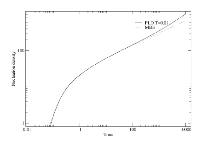
Figure 1: Numerical solution of the Eq. (1)with $d=2$ for PLD ($T=0.01$) and MBE (with the same parameters $F=I=D=1$, in arbitrary unit in order to illustrate the exponents). Notice the deviation of the PLD from MBE regime at $t_{c}=T^{-1}=100$ see Eq. 6

We illustrate our approach by Kinetic Monte-Carlo simulations (KMC). In  Xu a clear KMC realization has been presented, quite in accord with what has been presented in the present paper. For the KMC simulations we have a d-dimensional lattice and process as following: $I$ adatoms are deposited on each pulse, between the pulses we choose randomly an adatom and moves it randomly in one of the $2d$ possible directions. The comparison between the solution of the rate equation with the Monte-Carlo simulation is performed with two assumptions. First, we measure the nucleation density in the Monte-Carlo simulation, i.e. the number of island creations per-unit surface(neglecting reaction rates with more than two particles, the nucleation density is the same as $N$). Second, we consider the limit $T\rightarrow\infty$($t$ kept constant), and in order to simulate this limit we deposit $I$ adatoms(only on free sites on the grid) and when all adatoms have merged (an adatom is the neighbor of an occupied site, sticks and does not diffuse anymore ) to an island or an adatom, i.e. $N_{1}(t)=0$ then $I$ adatoms are deposited (during the lapse time of deposition of $I$ adatoms, the adatoms do not diffuse). In this regime the computation of the asymptotic value is simpler (see Fig. 2 and Fig. 3(the evolution for $t>0.01$ cannot be describes by our model. The author supposes that it could be finite-size effect or coalescence)) and we get the non-trivial scaling behavior $t^{0.5}$ for the immobile island density $N$.

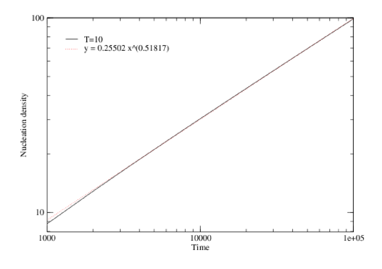
Figure 2: Kinetic Monte-carlo simulation in $d=1$. Nucleation density for $T=\infty$, $d=1$. The best approximation (the dashed line given by $Xmgrace$) has the exponent $\approx 0.518$

.

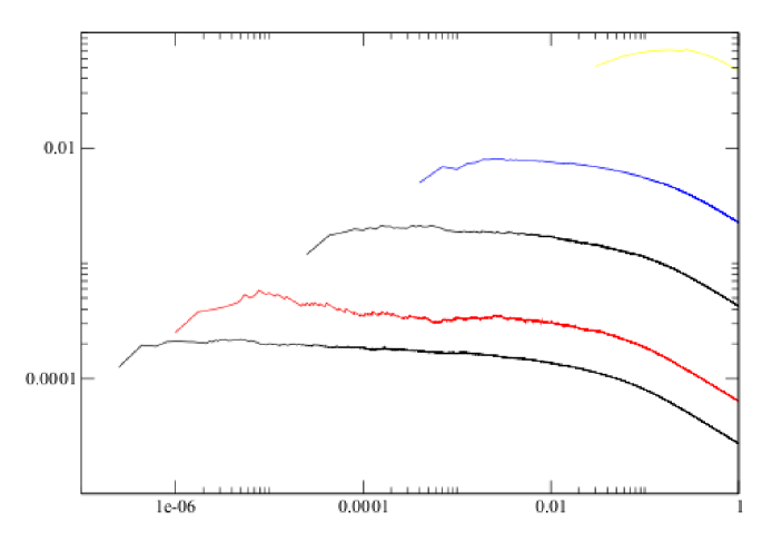
Figure 3: Kinetic Monte-carlo simulation in $d=2$. Nucleation density divided by $t^{0.5}$ for $T=\infty$ and dimension $d=2$, with the density of deposited adatoms per pulse $I=10^{-7},10^{-6},10^{-5},10^{-4},10^{-2}$ from the lowermost to the uppermost curve as function of time.

V Conclusion and outlooks

In this paper we have shown that a pulsed input of particle yields a very different solution of the immobile cluster density. We propose a different type of crossover. We hope to find some experimental evidence of this scaling and crossover. The author hopes that this approach will lead to similar result when for instance the deposition time of particle is not as small in comparison to the time span between two pulses flux . In this case the rescaling of the rates equation will lead to a set of equation with two parameters, the author expects to find that in this case the PLD regime dominates for large time. The PLD regime would be hence a regime which generalizes the MBE regime.

References

- (1) D.B.Chrisey and G .K. Hubler(editors),Pulsed Laser Deposition, John wiley and Sons, New York(1994).
- (2) R. G. Meyerand, Jr. and A. F. Haught, Phys. Rev. Lett., 13, 7 9 (1964).
- (3) A. Tselev, A. Gorbunov, and W. Pompe,Rev. Sci. Inst., 72, 2665-2672 (2001).
- (4) T.Venkatesan, Pulsed Laser Deposition : future Trends in D.B. Chrisey and G.K.Hubler(editors),Pulsed Laser Deposition, John wiley and Sons, New York(1994).
- (5) F.Westerhoff, L. Brendel and D.E. Wolf, in Structure and Dynamics of heterogeneous Systems, edited by P.Entel and D.E. Wolf ( World Scientific, singapore, 2000).
- (6) W. Matthew, Epitaxial Growth, (Academic, New York, 1975)
- (7) J.Y. Tao, Materials Fundamentals of Molecular Beam Epitaxy, (World Scientific, singapore, 1993).
- (8) J.G Amar, F. Family and P.-M. Lam, Phys. Rev. B50, 8781(1998).
- (9) B. Hinnemann, H. Hinrichsen, and D. E. Wolf Phys. Rev. Lett. 87, 135701 (2001).
- (10) L.Sittler and H. Hinrichsen,J. Phys. A 35, 10531-10538 (2002).
- (11) M.J. Aziz,Appl. Phys. A, 93,579 (2008).
- (12) T.Michely and J.Krug , Atoms islands and mounds (Springer, 2004).
- (13) J.W.Evans, R.Thiel, and M.C.Bartelt, Surf. Sci. Rep.,61 (2006).
- (14) J.A. Blackman, P.A. Mulheran, Phys.Rev. B,54 (1996) 11681.
- (15) J.G. Amar, M.N. Popescu, and F. Family, Surf. Sci. ,491, p.239-254 (2001).
- (16) M.C.Bartelt and J.W.Evans, Phys. Rev. B,54 (1996) R17359.
- (17) A. C. Barato, H. Hinrichsen, and D. E. Wolf Phys. Rev. E77, 041607 (2008).
- (18) L.Sittler J. Phys. A 41, 055005 (2008).
- (19) A. Pimpinelli, J. Vilain, and D.E. Wolf ,Phys. Rev. Lett. , 69 985, (1992).
- (20) M.C.Bartelt and J.W.Evans, Phys. Rev.,B46 (1992) 12675.
- (21) P.Jensen and B. Niemeyer,Surf. Sci.384,L823-L827 (1997).
- (22) S.Schinzer, M.Sokolowski, M. Biehl and W.KinzelPhys. Rev. B, 60, 2893 (1999).
- (23) N.Combes and P.JensenPhys. Rev. B,57 15553(1998).
- (24) V.A. Arnol’d Method of classical mechanics Springer Verlag (1980).
- (25) X.-J. Zhen, Bo Yan, Z. Zhu, B. Wu,and Y.-L. Mao.,Thin Solid Films,515 (2006) 2754 2759.