Resolving Curvature Singularities in Holomorphic Gravity

Abstract

We formulate holomorphic theory of gravity and study how the holomorphy symmetry alters the two most important singular solutions of general relativity: black holes and cosmology. We show that typical observers (freely) falling into a holomorphic black hole do not encounter a curvature singularity. Likewise, typical observers do not experience Big Bang singularity. Unlike Hermitian gravity MantzHermitianGravity , Holomorphic gravity does not respect the reciprocity symmetry and thus it is mainly a toy model for a gravity theory formulated on complex space-times. Yet it is a model that deserves a closer investigation since in many aspects it resembles Hermitian gravity and yet calculations are simpler. We have indications that holomorphic gravity reduces to the laws of general relativity correctly at large distance scales.

I Introduction

The existence of singularities in Einstein’s well tested theory of general relativity have puzzled many physicists since their discovery. It is a goal of (and motivation for) theories as quantum gravity to remove them. We propose generalizations of general relativity which to a great extent ease the singularity problems already at the classical level of the theory. Singularities of general relativity are typically manifest as divergences of some curvature invariant and are ubiquitous in general relativity Hawking:1973uf ; Wald:1984rg .

Consider, for example, the Big Bang singularity. A universe undergoing a power-law expansion expands with a scale factor, $a\sim t^{1/\epsilon}$, where $\epsilon=-\dot{H}/H^{2}={\rm constant}\geq 0$ denotes the ‘slow roll’ parameter, $H=\dot{a}/a$ is the Hubble expansion rate and dot denotes a derivative with respect to physical time $t$. The Ricci scalar $R$ then diverges as $t\rightarrow 0$ (corresponding to the time when matter density diverges),

$$R=6(2-\epsilon)H^{2}=\frac{6(2-\epsilon)}{\epsilon^{2}t^{2}}\rightarrow\infty\,,\qquad{\rm as}\;\;t\rightarrow 0\,.$$ (1)

Analogously, the Schwarzschild metric is singular when the coordinate radius $r=\|\vec{x}\|\rightarrow 0$ (corresponding to the place where all of the mass is concentrated), resulting in the curvature singularity of the Riemann tensor,

$$R_{\mu\nu\rho\sigma}R^{\mu\nu\rho\sigma}=\frac{48G_{N}^{2}M^{2}}{c^{4}r^{6}}\rightarrow\infty\,,\qquad{\rm as}\;\;r\rightarrow 0\,,$$ (2)

where $M$ denotes the black hole mass, $G_{N}$ the Newton constant and $c$ the speed of light.

On complex manifolds space-time coordinates $x^{\mu}$ get complexified as MantzHermitianGravity , 

$$x^{\mu}\rightarrow z^{\mu}=x^{\mu}+iy^{\mu}\,,\qquad y^{\mu}=\frac{G_{N}}{c^{3}}p^{\mu}\,,$$ (3)

where $p^{\mu}$ denotes the energy-momentum four-vector of noninertial frames, which can take any value; for an on-shell particle/observer however, $p^{\mu}$ reduces to the particle’s energy-momentum. Based on the holomorphy symmetry, we expect that the singularities (1–2) appear as some power of

$$\frac{1}{z},$$ (4)

(and possibly its complex conjugate), where $z\rightarrow z^{0}=x^{0}+iy^{0}=x^{0}+i(G_{N}/c^{4})E$ for the Big Bang singularity (1) and $z\rightarrow\|\vec{z}\,\|=\|\vec{x}\|+i\|\vec{y}\,\|=\|\vec{x}\|+i(G_{N}/c^{3})\|\vec{p}\,\|$ for the black hole singularity (2). Near singularities the observed space-time curvature is typically proportional to a power of the real part of (4),

$$\Re\bigg{[}\frac{1}{z}\bigg{]}=\frac{x}{x^{2}+y^{2}},$$

which blows up only when both $x$ and $y$ are simultaneously zero. The aim is now to formulate a generalization of general relativity that yields such complexified singularities and show that for a freely falling observer $x$ and $y$ are almost never zero simultaneously.  In Hermitian gravity MantzHermitianGravity , the Big Bang singularity can be considered as ‘resolved’ in the sense that the set of observers moving backwards in time that encounter the Big Bang singularity is of measure zero. So typical observers do not see the singularity. Note that this is not the case in general relativity, where all backward-moving observers eventually hit the Bing Bang singularity. In this paper we present a new theory, holomorphic gravity, in which also typical observers falling into a Schwarzschild black hole do not encounter a singularity. We believe that this resolution of singularities is a generic feature of gravity theories formulated on complex spaces as presented in this work and in Ref. MantzHermitianGravity , representing one of the principal advantages of complex theories of gravity when compared with Einstein’s general relativity.

II Almost Complex Structure

A natural generalization of general relativity, in order to obtain complex solutions as (4), would be to consider a theory with complex metrics, living on complex manifolds. A general complex metric on a complex manifold is given by

$$C=C_{\mu\nu}dz^{\mu}\otimes dz^{\nu} + C_{\mu\bar{\nu}}dz^{\mu}\otimes dz^{\bar{\nu}}$$ (5)

$$+C_{\bar{\mu}\nu}dz^{\bar{\mu}}\otimes dz^{\nu} + C_{\bar{\mu}\bar{\nu}}dz^{\bar{\mu}}\otimes dz^{\bar{\nu}},$$

where barred indices $z^{\bar{\mu}}\equiv{\bar{z}}^{\mu}$ denote complex conjugation. Hermitian gravity MantzHermitianGravity is formulated on a Hermitian manifold endowed with a Hermitian metric, defined as follows

$$C_{p}\left(J_{p}Z,J_{p}W\right)=C_{p}\left(Z,W\right)\,,$$ (6)

where the action of the almost complex structure operator, $J$, on the basis vectors of the complexified tangent space is given by

$$J_{p}\left(\frac{\partial}{\partial z^{\mu}}\right)=i\frac{\partial}{\partial z^{\mu}}\phantom{halloda}J_{p}\left(\frac{\partial}{\partial\bar{z}^{\mu}}\right)=-i\frac{\partial}{\partial\bar{z}^{\mu}}.$$ (7)

A Hermitian metric is a complex metric which has – as a consequence of the symmetry requirement (6) – vanishing $C_{\mu\nu}$ and $C_{\bar{\mu}\bar{\nu}}$ components:

$$C=C_{\mu\bar{\nu}}dz^{\mu}\otimes dz^{\bar{\nu}}+C_{\bar{\mu}\nu}dz^{\bar{\mu}}\otimes dz^{\nu}\,.$$

The requirement that the complex metric satisfies Bianchi identities lead us in MantzHermitianGravity to the conclusion that Eq. (6) can be consistently imposed on the metric only at the level of the equations of motion (on-shell), while at the level of the action (off-shell) all complex metrics of the form (5) are in fact allowed. Thus studying holomorphic gravity allows one also to rectify the differences between the full complex theory (which, apart from holomorphy on vielbeins, has no additional symmetry requirements) and hermitian gravity.

One of the reasons why one wants to study a theory of gravity that is invariant under the operation of $J$, is that the commutation relations of quantum mechanics are invariant under its action, which seems an invitation for quantization (recall that the $y^{\mu}$ coordinate in (3) is identified with the energy-momentum coordinate, $p^{\mu}$, in the commutation relations).

We can also consider the theory which is anti-symmetric under the action of the almost complex structure operator, in the sense that the holomorphic metric is defined in the following manner

$$C_{p}\left(J_{p}Z,J_{p}W\right)=-C_{p}\left(Z,W\right).$$ (8)

The holomorphic metric can then be written as

$$C=C_{\mu\nu}dz^{\mu}\otimes dz^{\nu}+C_{\bar{\mu}\bar{\nu}}dz^{\bar{\mu}}\otimes dz^{\bar{\nu}},$$ (9)

where the component $C_{\mu\nu}$ ($C_{\bar{\mu}\bar{\nu}}$ ) is (anti-)holomorphic, which simplifies calculations. In the remainder of this paper we construct a theory of gravity, based on the holomorphic metric (9). In the flat space limit the holomorphic metric is invariant under the complexified Lorentz group, $SO(1,3;\mathbb{C})$, while the line element is invariant under the complexified inhomogeneous Lorentz group (the complexified Poincaré group) $ISO(1,3;\mathbb{C})$.

III The Holomorphic Metric

The holomorphic line element is defined in the following manner

$$ds^{2}=dz^{\mu}C_{\mu\nu}dz^{\nu}+dz^{\bar{\mu}}C_{\bar{\mu}\bar{\nu}}dz^{\bar{\nu}},$$ (10)

which can be written in eight dimensional notation

$$ds^{2}=d\boldsymbol{z}^{T}\cdot\boldsymbol{C}\cdot d\boldsymbol{z}=(d\boldsymbol{z}^{m})^{T}\boldsymbol{C}_{mn}d\boldsymbol{z}^{n}$$

$$=(dz^{\mu},dz^{\bar{\mu}})\left(\begin{array}[]{cc}C_{\mu\nu}&0\\ 0&C_{\bar{\mu}\bar{\nu}}\end{array}\right)\left(\begin{array}[]{c}dz^{\nu}\\ dz^{\bar{\nu}}\end{array}\right),$$ (15)

where the Latin indices can take the values $0,1,...,$$d-1$,$\bar{0},\bar{1},...,\overline{d-1}$, the Greek indices run in the range $0,1,...,d-1$ and $d$ denotes the complex dimension of the complex manifold. The entries of the metric $\bm{C}_{mn}$ are functions of holomorphic and antiholomorphic vielbeins defined as follows 

$$C_{\mu\nu}=e(z)^{\phantom{\mu}a}_{\mu}\eta_{ab}e(z)^{\phantom{\mu}b}_{\nu}$$ (16)

$$C_{\bar{\mu}\bar{\nu}}=e(\bar{z})^{\phantom{\bar{\bar{\mu}}}a}_{\mu}\eta_{ab}e(\bar{z})^{\phantom{\mu}b}_{\bar{\nu}}.$$

The metric components are symmetric under transposition, since they are just an inner product of the vielbein times its transpose. Hence also in eight dimensional notation the metric is symmetric under transposition $\bm{C}^{T}=\bm{C}$. We define the $z^{\mu}$ and ${{z}}^{\bar{\mu}}$ coordinates in terms of $x^{\mu}$ and $y^{\check{\mu}}$, such that we obtain 

$$z^{\mu}=x^{\mu}+iy^{\check{\mu}}\,,\phantom{hallo}\frac{\partial}{\partial z^{\mu}} = \frac{1}{2}\Big{(}\frac{\partial}{\partial x^{\mu}}-i\frac{\partial}{\partial y^{\check{\mu}}}\Big{)}$$

and their complex conjugates. This implies the following decomposition of complex vielbeins in their real, ${e_{R}}^{a}_{\mu}$, and imaginary, ${e_{I}}^{a}_{\check{\mu}}$, parts in the following manner

$$e_{a}^{\mu} = {e_{R}}_{a}^{\mu}+i{e_{I}}_{a}^{\check{\mu}}\,,\phantom{hallo}\overline{e_{a}^{\mu}}=e_{a}^{\bar{\mu}}={e_{R}}_{a}^{\mu}-i{e_{I}}_{a}^{\check{\mu}}$$

$$e^{a}_{\mu} = {e_{R}}^{a}_{\mu}-i{e_{I}}^{a}_{\check{\mu}}\,,\phantom{hallo}\overline{e^{a}_{\mu}}=e^{a}_{\bar{\mu}}={e_{R}}^{a}_{\mu}+i{e_{I}}^{a}_{\check{\mu}}.$$ (17)

Vielbeins are holomorphic functions, and thus transform as holomorphic vectors (we consider only the transformation of the Greek indices for this purpose),

$$e_{\mu}^{a}(z^{\nu})\rightarrow\tilde{e}_{\mu}^{a}(w^{\nu})=\frac{\partial z^{\alpha}(w^{\nu})}{\partial w^{\mu}}e_{\alpha}^{a}(z^{\rho})$$ (18)

$$e^{\mu}_{a}(z^{\nu})\rightarrow\tilde{e}^{\mu}_{b}(w^{\nu})=\frac{\partial w^{\mu}(z^{\nu})}{\partial z^{\alpha}}e^{\alpha}_{b}(z^{\rho})\,.$$

The holomorphy of vielbeins,

$$\frac{\partial}{\partial z^{\bar{\mu}}}e_{\nu}^{a}=\frac{1}{2}\Big{[}\frac{\partial}{\partial{x^{\mu}}}+i\frac{\partial}{\partial y^{\check{\mu}}}\Big{]}[{e_{R}}_{\nu}^{a}+i{e_{I}}_{\check{\nu}}^{a}]=0\,,$$

implies the Cauchy-Riemann equations,

$$\frac{\partial{e_{R}}_{\nu}^{a}}{\partial x^{\mu}}=\frac{\partial{e_{I}}_{\check{\nu}}^{a}}{\partial y^{\check{\mu}}}\,,\qquad\frac{\partial{e_{I}}_{\check{\nu}}^{a}}{\partial x^{\mu}}=-\frac{\partial{e_{R}}_{\nu}^{a}}{\partial y^{\check{\mu}}}\,.$$ (19)

When rotating the metric from $z$ and $\bar{z}$ space to $x$ and $y$ space, the components of the holomorphic rotated metric $\bm{g}_{mn}$ are given by

$$\bm{g}_{mn}=\left(\begin{array}[]{cc}g_{\mu\nu}&g_{\mu\check{\nu}}\\[2.84544pt] g_{\check{\mu}\nu}&g_{\check{\mu}\check{\nu}}\end{array}\right)=\frac{1}{2}\left(\begin{array}[]{cc}C_{\mu\nu}+C_{\bar{\mu}\bar{\nu}}&i(C_{\mu\nu}-C_{\bar{\mu}\bar{\nu}})\\[2.84544pt] i(C_{\mu\nu}-C_{\bar{\mu}\bar{\nu}})&-C_{\mu\nu}-C_{\bar{\mu}\bar{\nu}}\end{array}\right)\,.$$ (24)

Its inverse then becomes

$$\bm{g}^{mn}=\frac{1}{2}\left(\begin{array}[]{cc}C^{\mu\nu}+C^{\bar{\mu}\bar{\nu}}&i(-C^{\mu\nu}+C^{\bar{\mu}\bar{\nu}})\\[2.84544pt] i(-C^{\mu\nu}+C^{\bar{\mu}\bar{\nu}})&-C^{\mu\nu}-C^{\bar{\mu}\bar{\nu}}\end{array}\right).$$ (27)

Clearly the entries of these rotated metrics are all symmetric and real. It is easily verified that $C_{\mu\nu}=g_{\mu\nu}-iK_{\mu\nu}$ and that $C_{\bar{\mu}\bar{\nu}}=g_{\mu\nu}+iK_{\mu\nu}$, $K_{\mu\nu}=g_{\mu\check{\nu}}=g_{\check{\mu}\nu}$ is a symmetric metric tensor and $g_{\check{\mu}\check{\nu}}=-g_{\mu\nu}$. We can write the metric in terms of the real and imaginary parts of the vielbein and in terms of the imaginary part of $C_{\mu\nu}$, using the definition of the complex metric in terms of vielbeins (16), yields

$$\boldsymbol{g}_{mn}=\left(\begin{array}[]{cc}e_{\mu}e_{\nu}-e_{\check{\mu}}e_{\check{\nu}}&-e_{\check{\mu}}e_{\nu}-e_{\mu}e_{\check{\nu}}\\[2.84544pt] -e_{\check{\mu}}e_{\nu}-e_{\mu}e_{\check{\nu}}&-e_{\mu}e_{\nu}+e_{\check{\mu}}e_{\check{\nu}}\end{array}\right).$$ (30)

Expressing the inverse metric $\boldsymbol{g}^{mn}$ in terms of vielbeins yields

$$\left(\begin{array}[]{cc}g^{\mu\nu}&K^{\mu\nu}\\[2.84544pt] K^{\mu\nu}&-g^{\mu\nu}\end{array}\right)=\left(\begin{array}[]{cc}e^{\mu}e^{\nu}-e^{\check{\mu}}e^{\check{\nu}}&e^{\check{\mu}}e^{\nu}+e^{\mu}e^{\check{\nu}}\\[2.84544pt] e^{\check{\mu}}e^{\nu}+e^{\mu}e^{\check{\nu}}&-e^{\mu}e^{\nu}+e^{\check{\mu}}e^{\check{\nu}}\end{array}\right).$$ (35)

With the rotated metric we can write down the holomorphic line element in its rotated form

$$ds^{2}=g_{\mu\nu}dx^{\mu}dx^{\nu}-\frac{2G_{N}}{c^{3}}K_{\mu\nu}dp^{\mu}dx^{\nu}-\frac{G_{N}^{2}}{c^{6}}g_{\mu\nu}dp^{\mu}dp^{\nu}\,.$$ (36)

From the definition of the complex metric in terms of vielbeins (16) and the fact that the vielbeins are defined to satisfy

$$e^{\mu}_{a}e^{a}_{\nu}=\delta^{\mu}_{\nu},$$

it follows that $\bm{g}^{me}$ and $\bm{g}_{en}$ are inverses of each other

$$\bm{g}^{me}\bm{g}_{en}=\bm{\delta}^{m}_{n},$$

where $\bm{\delta}^{m}_{n}$ is defined as

$$\bm{\delta}^{m}_{n}\equiv\left(\begin{array}[]{cc}\delta^{\mu}_{\nu}&0\\ 0&\delta^{\bar{\mu}}_{\bar{\nu}}\end{array}\right).$$ (39)

IV Flat Space

The holomorphic line element (36) in flat space becomes

$$ds^{2}=-(cdt)^{2}+(d\vec{x})^{2}-[-(dy^{0})^{2}+(d\vec{y})^{2}]\,.$$ (40)

Recall that the $y$ coordinate is related to the energy-momentum coordinate MantzHermitianGravity ; Low:2006qm as $y^{\mu}\equiv p^{\mu}{G_{N}}/{c^{3}}$. The space-time-momentum-energy interval squared from the origin to a space-time-momentum-energy point ${\bm{x}}^{m}$ is given by

$$d^{2}\left(\bm{0};{\bm{x}}^{m}\right)=-(ct)^{2}+(\vec{x})^{2}-\frac{G_{N}^{2}}{c^{6}}\left[-\left(\frac{E}{c}\right)^{2}+(\vec{p})^{2}\right]\,.$$ (41)

Note that the contribution of momentum-energy to the line element multiplies ${G_{N}^{2}}/{c^{6}}$, which is tiny (${G_{N}^{2}}/{c^{6}}\sim 10^{-72}{\rm s^{2}/kg^{2}}$), as it should be, since one does not observe any momentum-energy contribution to (41) at low energies. For light-like propagation ($ds^{2}=0$) and in the absence of momentum-energy contribution, Eq. (41) reduces to the well known result: massless particles move on the light-cone with the speed of light, $v=\|d\vec{x}/dt\|=c$.

On the other hand, for a light-like propagation in the presence of a non-vanishing momentum-energy contributions however, Eq. (41) yields,

$$-(ct)^{2}+(\vec{x})^{2}-\frac{p^{2}G_{N}^{2}}{c^{6}}=0,$$ (42)

where the variable $p^{2}=\eta_{\mu\nu}p^{\mu}p^{\nu}$ is the energy-momentum squared in a space-time-momentum-energy hyper-surface. Setting the space-time-momentum-energy interval to zero determines the boundary of causality (light cones). We can specify our hyper-surface further by setting $t$ to zero. Assuming $p^{2}>0$, one finds that there is a spatial region which is in instantaneous causal contact, and whose radius is given by,

$$r_{max}=\frac{\sqrt{p^{2}}G_{N}}{c^{3}}\qquad(p^{2}>0)\,.$$

The causally related regions (time-like, $ds^{2}<0$) for the case $p^{2}>0$ are shown as white in figure 1, where the region of non-local causal contact at $t=0$ is clearly seen as the hyperbola’s throat.

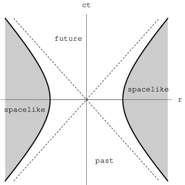
Figure 1: The figure shows how the light cones get modified by non inertial coordinate transformations on a space-time-momentum-energy diagram in the case when $p^{2}>0$. Note that there is a non-local instantaneous causally related volume element near the origin.

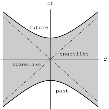
Figure 2: The figure shows how the light cones get modified by non-inertial coordinate transformations when $p^{2}<0$. There is a minimum time interval required for events to be in causal contact.

On the other hand, when $p^{2}<0$, the causal boundaries, shown in figure 2, are quite different. There is a minimal time $t_{min}$ required for events to be in causal contact,

$$t_{min}=\frac{\sqrt{-p^{2}}G_{N}}{c^{4}}\qquad(p^{2}<0)\,.$$

We now calculate the phase velocity, using the space-time-momentum-energy line element (42)

$$v_{\rm phase}=\frac{x}{t}=\sqrt{c^{2}+\frac{p^{2}G_{N}^{2}}{c^{4}t^{2}}}.$$ (43)

One can see that the phase velocity approaches the speed of light for large $t$.

On the other hand, the group velocity becomes

$$v_{g}=\sqrt{c^{2}+\frac{G_{N}^{2}}{c^{6}}f^{2}}\,,$$ (44)

where

$$f^{2}=-\frac{1}{c^{2}}\left(\frac{dE}{dt}\right)^{2}+\left(\frac{d\vec{p}}{dt}\right)^{2}\,.$$

The group velocity approaches the speed of light for small four-forces squared. Requiring that $v_{g}$ be real and positive (as required by propagation) sets a lower limit on the four force, $f^{2}\geq-c^{8}/G_{N}^{2}$. This is to be contrasted with an upper limit occurring in Hermitian gravity MantzHermitianGravity . Just like in the case of Hermitian gravity, we expect that these aparent violations of causality become of importance only in the regions where the particle’s self-gravity is large (in the vicinity of particle’s own event horizon).

V Second Order Formalism

Let us now state the holomorphic Einstein-Hilbert action, 

$$S=\frac{c^{4}}{16\pi G_{N}}\int d^{8}z\sqrt{-C}R+{\rm c.c.}$$ (45)

The holomorphic Ricci scalar is defined by $R=C^{\mu\nu}R_{\mu\nu}$, where the holomorphic Ricci tensor is given by

$$R^{\lambda}_{\mu\lambda\nu}=\partial_{\lambda}\Gamma^{\lambda}_{\nu\mu}-\partial_{\nu}\Gamma^{\lambda}_{\lambda\mu}+\Gamma^{\lambda}_{\lambda\alpha}\Gamma^{\alpha}_{\nu\mu}-\Gamma^{\lambda}_{\nu\alpha}\Gamma^{\alpha}_{\lambda\mu}\,,$$ (46)

and where here $\partial_{\lambda}={\partial}/{\partial z^{\lambda}}$. Since the holomorphic Einstein-Hilbert action is just the complexified equivalent of the Einstein-Hilbert action of standard general relativity, the equations of motions for this theory are just complexified equivalents of the equations of motions of general relativity. Using first order formalism MantzThesis:2007 , the equations of motion implied by the action (45) are:

$$G_{\mu\nu} = \frac{8\pi G_{N}}{c^{4}}T_{\mu\nu}$$ (47a)

$$\nabla_{\rho}C^{\mu\nu} = 0\,.$$ (47b)

Through the holomorphic metric compatibility equations (47b) the holomorphic connection coefficients are given by

$$\Gamma_{\mu\nu}^{\rho}=\frac{1}{2}C^{\rho\epsilon}(\partial_{\mu}C_{\epsilon\nu}+\partial_{\nu}C_{\mu\epsilon}-\partial_{\epsilon}C_{\mu\nu})\,.$$ (48)

Plugging the holomorphic Levi-Cività connection coefficients into the holomorphic Einstein’s equations (47a), we obtain second order differential equations in terms of the holomorphic metric only.

When varying the holomorphic line element (15) we obtain the following holomorphic geodesic equations

$$\ddot{z}^{\rho}+\Gamma_{\mu\nu}^{\rho}\dot{z}^{\mu}\dot{z}^{\nu}=0$$ (49)

and its complex conjugate. We can write equations (49) in their convenient eight dimensional form, such that we can rotate them to $x,y$ space, by simply plugging in the rotated metric (35). This is possible because the holomorphic connection coefficients transform as a (1,2) tensor under the constant coordinate transformations such as rotations from $z,\bar{z}$ to $x,y$ space. The rotated eight dimensional connection coefficients are then simply given by

$${\bm{\Gamma}}_{mn}^{r}=\frac{1}{2}{\bm{g}}^{re}(\partial_{m}{\bm{g}}_{en}+\partial_{n}{\bm{g}}_{me}-\partial_{e}{\bm{g}}_{mn})\,,$$ (50)

where the metric $\bm{g}_{mn}$ is just the eight dimensional rotated metric (24).

VI The Limit to General Relativity

The limit of Holomorphic gravity to general relativity is based on the assumption that the $y$ coordinate and its corresponding vielbein are small. When expanding the equations of holomorphic gravity in powers of $y$ and its corresponding vielbein, we hope to obtain the theory of general relativity at zeroth order of the expansion and meaningful corrections at linear order. The easiest way to obtain the limit to general relativity is to expand the vielbeins in terms of the $y$ coordinate

$$e_{\mu}^{a}(x,y)={\rm e}^{iy\cdot\partial_{x}}e_{\mu}^{a}(x)\,.$$ (51)

From this and the definition, $C_{\mu\nu}=e_{\mu}(z)\cdot e_{\nu}(z)$, we conclude that the analogous formula holds for the holomorphic metric tensor, $C_{\mu\nu}(x,y)={\rm e}^{iy\cdot\partial_{x}}C_{\mu\nu}(x)$, such that,

$$g_{\mu\nu}(x,y) = \;\;\;\cos\left(y\cdot\partial_{x}\right)g_{\mu\nu}(x)+\sin\left(y\cdot\partial_{x}\right)K_{\mu\nu}(x)$$

$$K_{\mu\nu}(x,y) = -\sin\left(y\cdot\partial_{x}\right)g_{\mu\nu}(x)+\cos\left(y\cdot\partial_{x}\right)K_{\mu\nu}(x)\,,$$

where we made use of Eqs. (24) and (35). The analogous relations hold for the inverses $g^{\mu\nu}$ and $K^{\mu\nu}$. Assuming that $K_{\mu\nu}$ is – just like $y^{\mu}$ – a first order quantity, Eq. (LABEL:gK:expand) then tells us that $g_{\mu\nu}(x,y)$ acquires corrections at second order in $y$, while $K_{\mu\nu}(x,y)$ acquires first order corrections in $y$, with $K_{\mu\nu}$ being on its own a first order quantity.

This analysis then implies that the connection with all indices unchecked yields the ordinary Levi-Cività connection plus corrections of second order

$$\Gamma^{\rho}_{\mu\nu}(x,y)=\Gamma^{\rho}_{\mu\nu}(x)+O(y^{2}).$$

With these connection coefficients, we can know check if the theory reduces to the theory of general relativity by plugging them into the rotated eight dimensional geodesic equation. Keeping only terms of linear order in the $y$ coordinate and its corresponding vielbein, yields the ordinary geodesic equation

$$\ddot{x}^{\rho}+\Gamma_{\mu\nu}^{\rho}(x){\dot{x}}^{\mu}{\dot{x}}^{\nu}+O(y^{2})=0$$

without any first order corrections present. We have not studied in detail the reduction of holomorphic Einstein’s equations to general relativity. Our study of holomophic Schwarzschild solution and cosmology in sections VII and VIII suggests however that holomorphic gravity reduces to Einstein’s theory in the low energy limit.

VI.1 Scalar Field

In this subsection we consider the following scalar field action

$$S_{\phi}=\int d^{8}z\sqrt{-C}\left[-\frac{1}{2}C^{\mu\nu}(\nabla_{\mu}\phi)\nabla_{\nu}\phi-V(\phi)\right]+{\rm c.c.}\,,$$ (53)

where $\phi=\phi(z^{\mu})$ is a holomorphic function of $z^{\mu}$. The equations of motion for the scalar field are then

$$\square\phi-\frac{dV}{d\phi}=0$$ (54)

and its complex conjugate, where $\square=C^{\mu\nu}\nabla_{\mu}\nabla_{\nu}$ and $\overline{\square}=C^{\bar{\mu}\bar{\nu}}\nabla_{\bar{\mu}}\nabla_{\bar{\nu}}$. When varying this action with respect to the metric we obtain the two sets of components of the stress-energy tensor

$$T_{\alpha\beta}=\nabla_{\alpha}\phi\nabla_{\beta}\phi-\frac{1}{2}C_{\alpha\beta}C^{\mu\nu}\nabla_{\mu}\phi\nabla_{\nu}\phi-C_{\alpha\beta}V(\phi)$$ (55)

and its complex conjugate. The energy conservation equations are

$$\nabla_{\mu}T^{\mu\nu}=\left(\square\phi-\frac{dV}{d\phi}\right)\nabla^{\nu}\phi=0$$

and its complex conjugate, where we have used Eq. (54). There are two sets of Einstein’s equations, namely

$$R_{\mu\nu}=\frac{8\pi G_{N}}{c^{4}}\left(\nabla_{\mu}\phi\nabla_{\nu}\phi+C_{\mu\nu}V(\phi)\right)$$ (56)

and again its complex conjugate. The energy-momentum tensor of a perfect fluid in the fluid rest frame can be written in the diagonal form

$$T^{\mu}_{\phantom{\mu}\nu}=\text{diag}(-\rho,p,p,p)$$ (57)

plus its complex conjugate, where $\rho$ is the density and $p$ the pressure. For a homogeneous scalar field $\phi=\phi(t)$, Eq. (55) yields, $\rho=(1/2c^{2})\dot{\phi}^{2}+V(\phi)$ and $p=(1/2c^{2})\dot{\phi}^{2}-V(\phi)$.

VII The holomorphic Schwarzschild Solution

The holomorphic Schwarzschild solution should just be a complexified version of the ordinary Schwarzschild solution, since the holomorphic Einstein’s equations (47a) are just complexified versions of the ordinary Einstein’s equations. So we expect to have the holomorphic metric components

$$C_{00}=-\left(1-\frac{1}{c^{2}}\frac{2G_{N}M}{z}\right)\,,$$

$$C_{11}=\left(1-\frac{1}{c^{2}}\frac{2G_{N}M}{z}\right)^{-1}$$ (58)

and their complex conjugates, where $z=\|\vec{z}\|=\|\vec{x}\|+i\frac{G_{N}}{c^{3}}\|\vec{p}\|\equiv r+i\frac{G_{N}}{c^{3}}p$ and $M$ is the mass of the black hole, which in holomorphic gravity could, in principle, be complex.  The angular part takes the same form as in general relativity

$$d\Omega^{2}=d\theta^{2}+\text{sin}^{2}\theta d\phi^{2},$$ (59)

but now the spherical symmetry is $O(3;\mathbb{C})$ and thus the angular parameters are complex

$$\theta={\theta_{R}}+i{\theta_{I}}\phantom{hallo}\phi={\phi_{R}}+i{\phi_{I}}.$$

Thus the angular part of the holomorphic Schwarzschild solutions is the complex angular part (59) plus its complex conjugate. One can easily check that the holomorphic Schwarzschild solution is indeed a solution to the holomorphic Einstein’s equations (47a) in vacuüm. Expressing the Schwarzschild components (58) in $r$ and $p$ yields

$$C_{00} = -\left(1-\frac{2G_{N}M}{c^{2}}\frac{r-i\frac{G_{N}}{c^{3}}p}{r^{2}+\frac{G_{N}^{2}}{c^{6}}p^{2}}\right)$$

$$C_{11} = \frac{r^{2}+\frac{G_{N}^{2}}{c^{6}}p^{2}-\frac{2G_{N}M}{c^{2}}(r+i\frac{G_{N}}{c^{3}}p)}{(r-\frac{2G_{N}M}{c^{2}})^{2}+\frac{G_{N}^{2}}{c^{6}}p^{2}}=-\frac{1}{C_{00}}$$ (60)

and their complex conjugates. The rotated holomorphic metric components (24) are given in terms of the holomorphic metric components (60), and take the following form

$$g_{00} = -\left(1-\frac{2G_{N}M}{c^{2}}\frac{r}{r^{2}+\frac{G_{N}^{2}}{c^{6}}p^{2}}\right)$$

$$g_{11} = \frac{r^{2}+\frac{G_{N}^{2}}{c^{6}}p^{2}-\frac{2G_{N}M}{c^{2}}r}{(r-\frac{2G_{N}M}{c^{2}})^{2}+\frac{G_{N}^{2}}{c^{6}}p^{2}}$$

$$g_{0\check{0}} = \frac{\frac{2G_{N}^{2}M}{c^{5}}p}{r^{2}+\frac{G_{N}^{2}}{c^{6}}p^{2}}$$

$$g_{1\check{1}} = \frac{\frac{2G_{N}^{2}M}{c^{5}}p}{(r-\frac{2G_{N}M}{c^{2}})^{2}+\frac{G_{N}^{2}}{c^{6}}p^{2}}\,,$$

which reduces to the Schwarzschild solution of general relativity when $p\rightarrow 0$. When these rotated components are inserted into the rotated holomorphic line element (36), one obtains the holomorphic Schwarzschild metric in its full glory

$$ds^{2}=$$

$$-\left(1-\frac{2G_{N}M}{c^{2}}\frac{r}{r^{2}+\frac{G_{N}^{2}}{c^{6}}p^{2}}\right)\left[(cd{t})^{2}-\frac{G_{N}^{2}}{c^{8}}\left(dE\right)^{2}\right]$$

$$+\frac{r^{2}+\frac{G_{N}^{2}}{c^{6}}p^{2}-\frac{2G_{N}M}{c^{2}}r}{(r-\frac{2G_{N}M}{c^{2}})^{2}+\frac{G_{N}^{2}}{c^{6}}p^{2}}\left[(d{r})^{2}-\frac{G_{N}^{2}}{c^{6}}(d{p})^{2}\right]$$

$$+\frac{\frac{2G_{N}^{2}M}{c^{5}}p}{(r-\frac{2G_{N}M}{c^{2}})^{2}+\frac{G_{N}^{2}}{c^{6}}p^{2}}\frac{2G_{N}}{c^{3}}drdp$$

$$+\frac{\frac{2G_{N}^{2}M}{c^{5}}p}{r^{2}+\frac{G_{N}^{2}}{c^{6}}p^{2}}\frac{2G_{N}}{c^{4}}dtdE+\left(r^{2}-\frac{G_{N}^{2}}{c^{6}}p^{2}\right)\left(d{\theta_{R}}^{2}-d{\theta_{I}}^{2}\right)$$

$$-4\frac{G_{N}}{c^{3}}rpd{\theta_{R}}d{\theta_{I}}+\left(d{\phi_{R}}^{2}-d{\phi_{I}}^{2}\right)\times$$

$$\times\Big{[}\left(r^{2}-\frac{G_{N}^{2}}{c^{6}}p^{2}\right)\{(\text{sin}{\theta_{R}}\text{cosh}{\theta_{I}})^{2}-(\text{cos}{\theta_{R}}\text{sinh}{\theta_{I}})^{2}\}$$

$$-4\frac{G_{N}}{c^{3}}rp(\text{sin}{\theta_{R}}\text{cosh}{\theta_{I}}\text{cos}{\theta_{R}}\text{sinh}{\theta_{I}})\Big{]}$$

$$-2d{\phi_{R}}d{\phi_{I}}\Big{[}\left(r^{2}-\frac{G_{N}^{2}}{c^{6}}p^{2}\right)2\text{sin}{\theta_{R}}\text{cosh}{\theta_{I}}\text{cos}{\theta_{R}}\text{sinh}{\theta_{I}}$$

$$+2\frac{G_{N}}{c^{3}}rp\{(\text{sin}{\theta_{R}}\text{cosh}{\theta_{I}})^{2}-(\text{cos}{\theta_{R}}\text{sinh}{\theta_{I}})^{2}\}\Big{]}.$$

This rotated holomorphic Schwarzschild metric is indeed a solution of the rotated holomorphic Einstein’s equations in vacuüm, as can be checked by explicit calculation of $R_{\mu\nu}$. It is easy to see that, in the limit when the radius $r$ goes to infinity and $p$ to zero, the solution approaches the Minkowski metric, whereas the solution approaches the momentum-energy Minkowski space when $r$ goes to zero and $p$ goes to infinity. If $p$ is not zero when $r$ is zero, there is no curvature singularity at the origin. Explicit calculation shows that $p$ is not zero when $r$ is zero for a generic infalling observer. When considering an observer which is falling in radially we can neglect the change in angular coordinates, corresponding to a vanishing angular momentum. (Recall that in general relativity this choice corresponds to the worst case scenario, for which an observer descends in the quickest possible way towards the black hole singularity.) Based on the holomorphic Schwarzschild metric (58) the black hole line element (10) of a radially infalling observer can be recast as

$$-2c^{2}=- \left(1-\frac{1}{c^{2}}\frac{2G_{N}M}{z}\right)\left(\frac{dz^{0}}{d\tau}\right)^{2}$$

$$+ \left(1-\frac{1}{c^{2}}\frac{2G_{N}M}{z}\right)^{-1}\left(\frac{dz}{d\tau}\right)^{2}+\text{c.c,}\,,$$ (61)

where we introduced a real affine parameter (proper time) ${\tau}$ defined as $c^{2}(d\tau)^{2}=-ds^{2}$. The holomorphic Schwarzschild solution has an isometry in the $z^{0}$ direction ($\partial/\partial z^{0}$ is a Killing vector) and hence there is a conserved quantity:

$$e_{z}=u^{0}_{0}+i\frac{G_{N}}{c^{3}}f^{0}_{0}\,.$$ (62)

The real part $u^{0}_{0}=u^{0}(\tau_{0})$ corresponds to the (initial) zeroth component of the four-velocity evaluated at $\tau=\tau_{0}$ (the energy per unit mass divided by $c$), which is also the Killing vector in general relativity, while the imaginary part $f^{0}_{0}=f^{0}(\tau_{0})=(dp^{0}/d\tau)(\tau_{0})$ is the zeroth component of the observer’s four-force. Since $f^{0}_{0}$ does not contribute in general relativity, the general relativistic limit should be obtained by setting $f^{0}_{0}\rightarrow 0$, which is indeed the case. In analogy with general relativity, the conserved quantity can be written as Wald:1984rg

$$\left(\frac{dz^{0}}{d\tau}\right)^{2}=\left(1-\frac{1}{c^{2}}\frac{2G_{N}M}{z}\right)^{-2}e_{z}^{2}\,.$$ (63)

Equations (61) and (63) are not enough to fully determine $z=z(\tau)$, because nothing is known about the imaginary part of the expressions appearing in Eq. (61). Since we are in holomorphic gravity, it is reasonable to demand $z=z(\tau)$ to be a holomorphic function. With this analytic extension we can now completely determine $z=z(\tau)$ by inserting the conserved integral (63) into (61), to obtain

$$\left(\frac{dz}{cd\tau}\right)^{2}=b+\frac{r_{s}}{z}\,,\qquad b=\frac{e_{z}^{2}}{c^{2}}-1\,,\qquad r_{s}=\frac{2G_{N}M}{c^{2}}$$ (64)

and the complex conjugate of this equation. Note that $r_{s}$ is just the Schwarzschild radius and the on-shell value of $b=b_{r}+ib_{i}$ can be expressed in terms of the initial 3-velocity, $b_{r}=\gamma_{0}^{2}-1=(\gamma_{0}\vec{v}_{0}/c)^{2}$, $\gamma_{0}^{-2}=1-(\vec{v}_{0}/c)^{2}$. Solving (64) for proper time $\tau$ yields

$$\frac{c\tau}{r_{s}} =\frac{1}{b}\sqrt{\zeta(1+b\zeta)}$$

$$-\frac{1}{b^{\frac{3}{2}}}\text{ln}\left\{\sqrt{b\zeta}+\sqrt{1+b\zeta}\right\}\,,\quad\zeta=\frac{z}{r_{s}}\,.$$

From this it follows that, when $b$ is complex and $r\rightarrow 0$, $p$ is not zero. Moreover, one can show that quite generically, when $r\rightarrow 0$, $p$ grows large, which limits the growth of the curvature invariant (2), which for Holomorphic gravity has the simple generalization,

$$R_{\mu\nu\rho\sigma}R^{\mu\nu\rho\sigma}=\frac{12r_{s}^{2}}{z^{6}}\,.$$ (65)

For example, when $r\rightarrow 0$, this reduces to $R_{\mu\nu\rho\sigma}R^{\mu\nu\rho\sigma}\rightarrow-12c^{18}r_{s}^{2}/(G_{N}p)^{6}$, which is negative.

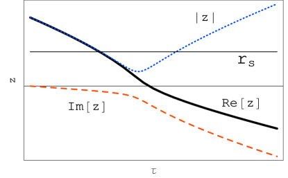
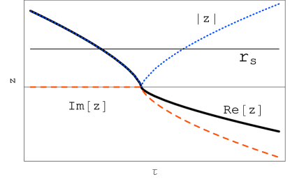
Figure 3: The real and imaginary part and the absolute value of the complex radial coordinate $z$ as a function of proper time $\tau$ for a freely falling observer for different initial conditions $b$. 3 The real and imaginary part and the absolute value of $z$ with a complex initial condition $b$. In this case $|z|=0$ is never reached, indicating that the observer encounters no black hole singularity. 3 The real and imaginary part and the absolute value of $z$ for a real initial $b$. In this case both $\Re[z]$ and $\Im[z]$ reach simultaneously zero for some value of proper time $\tau$, indicating a black hole singularity.

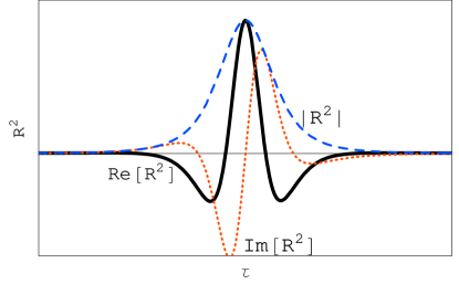
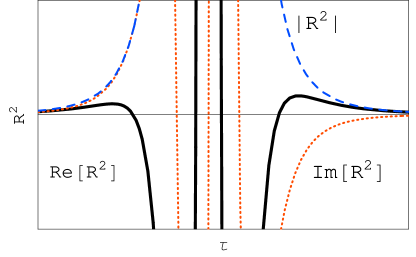
Figure 4: The real and imaginary part and the absolute value of the curvature invariant (65), which we for simplicity denote in figures by $R^{2}$. as a function of proper time $\tau$ for different initial conditions $b$. An infinite curvature is attained only when $\Im[b]=0$, which represents a set of initial conditions of measure zero. Fig. 4 The real and imaginary part and the absolute value of the curvature invariant for complex initial conditions $b$. The curvature invariant remains finite at all times. Fig. 4 A part of the upper panel 4 zoomed in. At large distances the real part of the curvature invariant (solid black line) approaches the general relativistic solution, but close to and within the Schwarzschild radius the curvature exhibits a very different behavior, becoming even negative. The deviation from the general relativistic behavior becomes large only within the Schwarzschild radius and hence remains hidden behind the black hole horizon.

In order to verify the limited curvature conjecture, we solve (64) numerically. For initial conditions, where the imaginary part of $b$ is nonvanishing, $p$ is indeed nonzero when $r=0$, as can be seen from figure 3. In this case there is no curvature singularity. When $\Im[b]=0$ however, then $r$ and $p$ simultaneously go to zero, the geodesics end at a curvature singularity, just like in the case of general relativity. This situation is illustrated in figure 3. Even though numerical solution indicates that the evolution continues after $r=0=p$ is reached, at that point there is a branch point of the evolution, and the numerical integrator picks one of the Riemann sheets (this is indicated by the cuspy feature of the numerical solution at $r=p=0$ in figure 3). Moreover, at $r=0=p$ the curvature invariant (65) becomes singular, as can be seen in figure 5. Since $\Im[b]=0$ only when the initial force $f_{0}^{0}=0$ exactly, the set of initial conditions where $b$ is real is of measure zero, when compared to the set of all initial conditions, where $b$ can be an arbitrary complex number. Hence we conclude that the curvature singularity is not seen by most of infalling observers.

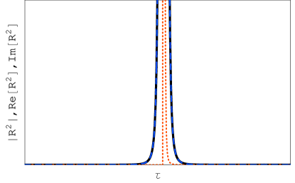
Figure 5: The real and imaginary part and the absolute value of the curvature invariant (65) with initial conditions corresponding to a real $b$ (vanishing initial force). Since $\Im[z]=0$ remains zero, the curvature invariant is identical to the corresponding curvature invariant in general relativity (1) such that a curvature singularity is reached at $r=0=p$.

Finally, we need to interpret what it means for $r$ to become negative, see figure 3. In the view of Eq. (64), for instance, we can take the sign out of the denominator and put it in the numerator

$$\frac{M}{-r+i(G_{N}/c^{3})p}=\frac{-M}{r-i(G_{N}/c^{3})p}\,.$$ (66)

In this way we effectively glue the holomorphic Schwarzschild solution with a negative $\Re[z]$ onto the anti-holomorphic solution with a positive $\Re[z]$ but with a negative mass: a white hole. This means that an observer can fall through a black hole and emerge from a white hole with an opposite momentum and v.v. Needless to say, this behavior is very different from general relativity, where classically nothing can come out once inside the event horizon. Finally, we note that the holomorphic and anti-holomorphic solutions are in general not symmetric under time reversal. This symmetry is broken, for example, by the imaginary part of the curvature invariant, as can be seen in figure 4.

VIII Cosmology

Since our Universe is isotropic and homogeneous on large scales, our complex generalized theory should also possess isotropy and homogeneity such that it reduces to the theory of general relativity correctly at low energies. Since our complex theories are completely specified in terms of vielbeins, an assumption concerning the vielbein modeling an isotropic and homogeneous universe is in place here. Let us try the following Ansatz:

$$e^{a}_{\mu}(z)=a(z_{c}^{0})\delta^{a}_{\mu}\phantom{hallo}e^{a}_{\bar{\mu}}(\bar{z})=\bar{a}\big{(}{z_{c}}^{\bar{0}}\big{)}\delta^{a}_{\bar{\mu}},$$ (67)

where

$$a(z_{c}^{0})=a_{R}(z_{c}^{0})+ia_{I}(z_{c}^{0})\phantom{hal}\bar{a}\big{(}z_{c}^{\bar{0}}\big{)}=a_{R}\big{(}z_{c}^{\bar{0}}\big{)}-ia_{I}\big{(}z_{c}^{\bar{0}}\big{)}\,,$$

where $z_{c}^{0}=\eta+iG_{N}E_{c}$ denotes a conformal complex ‘time.’ (In this section we set the speed of light $c=1$.) With these assumptions the holomorphic Christoffel symbols (48) are then given by

$$\Gamma^{\rho}_{\mu\nu}=\frac{a^{\prime}}{a}\left(\delta^{0}_{\nu}\delta^{\rho}_{\mu}+\delta^{0}_{\mu}\delta^{\rho}_{\nu}-\eta^{\rho 0}\eta_{\mu\nu}\right)\,$$ (68)

and its complex conjugate, where $a^{\prime}={da}/{dz_{c}^{0}}$. Inserting Eq. (68) into the holomorphic Riemann tensor (46) we obtain

$$R_{\mu\nu} = \left[\frac{a^{\prime\prime}}{a}-\left(\frac{a^{\prime}}{a}\right)^{2}\right]\left(\eta_{\mu\nu}-2\delta^{0}_{\nu}\delta^{0}_{\mu}\right)$$

$$+ \left(\frac{a^{\prime}}{a}\right)^{2}[2\delta^{0}_{\nu}\delta^{0}_{\mu}+2\eta_{\mu\nu}]$$

and its complex conjugate. The holomorphic Ricci scalars are then given by

$$R=6\frac{a^{\prime\prime}}{a^{3}}=6\left[\frac{\ddot{a}}{a}-\left(\frac{\dot{a}}{a}\right)^{2}\right]$$

and its complex conjugate, where we have contracted holomorphic Ricci tensors with the inverse metric $g^{\mu\nu}=({1}/{a^{2}})\eta^{\mu\nu}$ and its complex conjugate, and $\dot{a}={da}/{dz^{0}}$, $dz^{0}=adz_{c}^{0}$. The holomorphic Einstein’s equations in four dimensions are

$$R_{\mu\nu}=8\pi G_{N}(T_{\mu\nu}-\frac{1}{2}g_{\mu\nu}T)$$

and its complex conjugate, of course. Because of the isotropy and homogeneity symmetries imposed, the Einstein’s equations contain only four independent equations due to homogeneity and isotropy symmetries, namely one space-space ($ii$) equation,

$$\frac{\ddot{a}}{a}+2\left(\frac{\dot{a}}{a}\right)^{2}=4\pi G(\rho-p),$$ (69)

the time-time ($00$) equation,

$$\frac{\ddot{a}}{a}=-\frac{4\pi G}{3}(\rho+3p)$$ (70)

and the complex conjugates of these equations. We can simplify Eq. (69) by making use of the time component (70) to obtain

$$H^{2}\equiv\left(\frac{\dot{a}}{a}\right)^{2}=\frac{8\pi G_{N}}{3}\rho,$$ (71)

where $H={\dot{a}}/{a}$ denotes the holomorphic Hubble parameter. Equation (71) together with equation (70) constitute the holomorphic Friedmann equations. It is easy to see that the holomorphic Friedmann equations are consistent with the holomorphic energy conservation equations

$$\dot{\rho}+3\frac{\dot{a}}{a}(\rho+p)=0$$ (72)

and its complex conjugate, which is derived from the holomorphic energy conservation equations

$$\partial_{\mu}T^{\mu}_{\phantom{\lambda}0}+\Gamma^{\mu}_{\mu\lambda}T^{\lambda}_{\phantom{\lambda}0}-\Gamma^{\lambda}_{\mu 0}T^{\mu}_{\phantom{\lambda}\lambda}=0$$

and its complex conjugate, where we have used the expression of the energy-momentum tensor (57) and holomorphic Christoffel symbol (68). Making use of Eqs. (57) and (55), we can express the energy density $\rho$ and pressure $p$ in terms of the scalar field $\phi$. In an isotropic and homogeneous universe the scalar field is a holomorphic function of $z^{0}$, $\phi=\phi(z^{0})$, such that we have

$$\rho=\frac{1}{2}\dot{\phi}^{2}+V(\phi)\,,\qquad p=\frac{1}{2}\dot{\phi}^{2}-V(\phi).$$ (73)

The equations for $\bar{\rho}$ and $\bar{p}$ are just the complex conjugates of these expressions. The equation of motion for the scalar field (54) becomes

$$\ddot{\phi}+3H\dot{\phi}+\frac{dV}{d\phi}=0$$ (74)

and the holomorphic Friedmann equations (70–71) then become

$$\frac{\ddot{a}}{a}=-\frac{8\pi G_{N}}{3}\left({\dot{\phi}}^{2}-V\right)$$ (75)

and

$$H^{2}\equiv\left(\frac{\dot{a}}{a}\right)^{2}=\frac{8\pi G_{N}}{3}\left(\frac{\dot{\phi}^{2}}{2}+V\right)$$ (76)

and the corresponding complex conjugates. Just like in general relativity, one can show that only three equations among Eqs. (72) and (74–76) are independent.

We shall now study the holomorphic Friedmann equations for different physical circumstances and compare the results with those of general relativity.

VIII.1 Power law expansion

Let us now consider a homogeneous and holomorphic fluid with the equation of state,

$$w=\frac{p}{\rho}\,,\qquad w\in{\bm{C}}\,,\qquad\Re[w]\geq-1\,.$$ (77)

In this case Eq. (72) is solved by,

$$\rho=\frac{\rho_{0}}{a^{3(1+w)}}\,.$$ (78)

Next Eqs. (75) and (76) can be combined into,

$$\epsilon\equiv-\frac{\dot{H}}{H^{2}}=\frac{d}{dz^{0}}\left(\frac{1}{H}\right)=\frac{3}{2}(1+w)\,,$$ (79)

such that $\epsilon\in\bm{C}$ is a complex constant and $\Re[\epsilon]\geq 0$.

When equation (79) is integrated, one gets the holomorphic expansion rate,

$$H=\frac{1}{\epsilon z^{0}}\,.$$ (80)

This is easily integrated, to yield the holomorphic scale factor,

$$a=\left(\frac{z^{0}}{\zeta_{0}}\right)^{{1}/{\epsilon}}\,.$$ (81)

These solutions are a generalization of power law expansion of general relativity, in that $\epsilon$ is in general a complex parameter. $\zeta_{0}$ is an arbitrary constant parameter that signifies the complex time at which $a=1$. Its physical significance is revealed by realizing that $\zeta_{0}$ parametrizes the Hubble rate at the time $z^{0}=\zeta_{0}$, as can be seen from Eqs. (80) and (82).

Finally, the last equation we need to solve is (76), which gives,

$$H^{2}_{0}=\frac{1}{\epsilon^{2}\zeta_{0}^{2}}=\frac{8\pi G_{N}\rho_{0}}{3}\,,$$ (82)

where $H_{0}=H(\zeta_{0})$, $\rho_{0}=\rho(\zeta_{0})$.

We shall now show that, non unlike in general relativity, the holomorphic power law expansion (81) can be realised by a homogeneous holomorphic scalar field $\phi=\phi(z^{0})$ with an exponential potential. Just like in general relativity, the power law solution is then realised in the scaling limit, in which case it exhibits attractor behavior Ratra:1987rm .

Let us consider the following Lagrangian density

$${\cal L}=\frac{1}{2}{\dot{\phi}^{2}}-V(\phi)\,,\qquad V(\phi)=V_{0}\exp\left(-\lambda\frac{\phi}{M}\right)\,.$$ (83)

We now assume that the Friedmann equation permits a scaling solution of the form, $H\propto 1/z^{0}$. Obviously, such a solution must satisfy,

$$\dot{\phi}=\dot{\phi}_{0}\frac{\zeta_{0}}{z^{0}}\,,\qquad\phi=\phi_{0}+\dot{\phi}_{0}\zeta_{0}\ln\left(\frac{z^{0}}{\zeta_{0}}\right)\,,$$ (84)

where $\phi_{0},\dot{\phi}_{0}$ and $\zeta_{0}$ are (complex) constants (note that $\zeta_{0}$ and $\phi_{0}$ are not independent; indeed, rescaling $\zeta_{0}$ can be compensated by the appropriate shift in $\phi_{0}$). Note that Eq. (81) implies that the scalar field (84) can be considered as a ‘marker’ for the scale factor,

$$a=\exp\left(\frac{\phi-\phi_{0}}{\epsilon\dot{\phi}_{0}\zeta_{0}}\right)$$ (85)

and in this sense defines a clock.

A constant $w$ requires the scaling of the potential (83),

$$V=V_{0}\exp\left(-\frac{\lambda\phi_{0}}{M}\right)\left(\frac{\zeta_{0}}{z^{0}}\right)^{(\lambda\dot{\phi}_{0}\zeta_{0})/M}\,.$$ (86)

We are free to absorb $\phi_{0}$ in $V_{0}$ by redefining, $V_{0}\exp\left(-{\lambda\phi_{0}}/{M}\right)\rightarrow V_{0}$. Demanding the scaling,

$$V=V_{0}\left(\frac{\zeta_{0}}{z^{0}}\right)^{2}\,,$$ (87)

implies the following condition on the initial field velocity,

$$\dot{\phi}_{0}=\frac{2M}{\lambda\zeta_{0}}\,,$$ (88)

where $V_{0}=V(\phi_{0})=V(\phi(\zeta_{0}))$. 

Taking account of these scalings, the equation of state parameter $w$ becomes indeed constant,

$$w=\frac{\eta_{0}-1}{\eta_{0}+1}\,,\qquad\eta_{0}=\frac{\dot{\phi}_{0}^{2}}{2V_{0}}=\frac{2M^{2}}{\lambda^{2}V_{0}\zeta_{0}^{2}}$$ (89)

and hence $\epsilon$ in (79) is also constant,

$$\epsilon=\frac{d}{dz^{0}}\left(\frac{1}{H}\right)=\frac{3\eta_{0}}{1+\eta_{0}}\,.$$ (90)

The conservation equation is now trivially satisfied, implying the energy density scaling, $\rho=\rho_{0}/a^{2\epsilon}=\rho_{0}(\zeta_{0}/z^{0})^{2}$. Finally, the Friedmann equation (76) and (82) yields the constraint

$$H^{2}_{0}=\frac{8\pi G_{N}V_{0}}{3-\epsilon}\,.$$ (91)

When this is combined with Eq. (90), one gets the following algebraic equation for $\epsilon$

$$\epsilon\left(\epsilon-3\right)\left(\epsilon-\frac{\lambda^{2}}{16\pi G_{N}M^{2}}\right)=0\,,$$ (92)

which links the parameters of the scalar theory with $\epsilon$. Note that $\epsilon$ does not depend on the initial conditions on the field, but only on the coupling parameters of the potential. This should not surprise us since we are considering an attractor solution.

From Eq. (92) it follows that de Sitter space ($\epsilon=0$) and kination ($\epsilon=3)$ are solutions and have a special significance. One can show that $\Re[\epsilon]\leq 3$, the limit is saturated when $\lambda^{2}=16\pi G_{N}M^{2}$. For larger values of $\lambda$ there is no scaling solution: $V$ redshifts faster than the kinetic term, resulting in $\epsilon\rightarrow 3$. de Sitter space $\epsilon=0$ is also a solution of Eq. (92), which is realised when $\dot{\phi}_{0}=0$. This is indeed a stable solution, for which kinetic energy vanishes, and $V=V_{0}\equiv\Lambda_{0}/(8\pi G_{N})$, where $\Lambda_{0}$ denotes the equivalent cosmological constant, which in holomorphic gravity can be complex.

The nontrivial solution of Eq. (92) is

$$\epsilon=\frac{\lambda^{2}}{16\pi G_{N}M^{2}}\,,\qquad 0\leq\Re[\epsilon]\leq 3$$ (93)

which corresponds to the attractor solution when the condition $0\leq\Re[\epsilon]\leq 3$ in Eq. (93) is satisfied. Of course, the solution (93) is more general than the corresponding solution of general relativity in that $\lambda$ and hence also $\epsilon$ can be complex. To appreciate the significance of a complex $\epsilon$, let us assume that the Universe follows the attractor behavior with $\epsilon$ given by (93). In this case the exponential potential (83) can be written as ,

$$V\;\;\stackrel{{\scriptstyle\rm attractor}}{{\longrightarrow}}\;\;V_{0}\exp\left(-\sqrt{16\pi G_{N}\epsilon}\;\phi\right)\,,\qquad 0\leq\Re[\epsilon]\leq 3\,.$$ (94)

This potential can be used to obtain both an accelerating universe (for which $\Re[\epsilon]<1$) and a decelerating universe (with $\Re[\epsilon]>1$). Thus with the appropriate choice of $\lambda$ all standard cases in cosmology can be reproduced: radiation era ($\epsilon=2$); matter era ($\epsilon=3/2$); kination ($\epsilon=3$), which is realized in the limit when $\lambda\rightarrow 0$ and $V_{0}\rightarrow 0$; inflation ($0<\Re[\epsilon]\ll 1$), etc.

The physical Hubble parameter ${\cal H}$ is given in terms of the real part of the holomorphic expansion rate $H$ as, ${\cal H}^{2}=\Re[H^{2}]$. For a real $\epsilon$ Eq. (80) implies,

$$\Re[H^{2}]=\frac{t^{2}-G_{N}^{2}E^{2}}{\epsilon^{2}[t^{2}+G_{N}^{2}E^{2}]^{2}}\,.$$ (95)

For a complex $\epsilon$ the expression is more complicated,

$$\Re[H^{2}]=\frac{(\epsilon_{R}^{2}-\epsilon_{I}^{2})[t^{2}-G_{N}^{2}E^{2}]-4\epsilon_{R}\epsilon_{I}tG_{N}E}{|\epsilon|^{4}[t^{2}+G_{N}^{2}E^{2}]^{2}}.$$ (96)

In order to find out whether the holomorphic Big Bang singularity is ever reached, we need to study geodesic equations, which shall give us a crucial information on whether a freely falling observer experiences the holomorphic singularity in (95–96) (cf. Ref. MantzHermitianGravity ).

The physical scale factor ${\cal A}$ can be obtained as the real part of the holomorphic scale factor  (81) squared,

$${\cal A}^{2}=\left(\frac{t^{2}+G_{N}^{2}E^{2}}{|\zeta_{0}|^{2}}\right)^{\frac{\epsilon_{R}}{|\epsilon|^{2}}-\frac{\epsilon_{I}}{|\epsilon|^{2}}{\rm Arctan}\left(\frac{G_{N}E}{|t|}\right)}\times$$

$$\times\cos\Big{(}\left[\frac{2\epsilon_{I}}{|\epsilon|^{2}}+\frac{2\epsilon_{R}}{|\epsilon|^{2}}{\rm Arctan}\left(\frac{G_{N}E}{|t|}\right)\right]\times$$

$$\times\ln\left(\frac{t^{2}+G_{N}^{2}E^{2}}{|\zeta_{0}|^{2}}\right)\Big{)}\,,$$ (97)

where $\epsilon=\epsilon_{R}+i\epsilon_{I}$. When $\epsilon_{I}=0$ and provided $E$ does not grow with time (which is reasonable), the Universe approaches the standard FLRW cosmology. When however $\epsilon_{I}\neq 0$, the Universe’s scale factor develops oscillations, which can result in significant differences between holomorphic and FLRW cosmology even at late times. This is a disadvantage of holomorphic cosmology when compared with, for example, Hermitian cosmology developed in Ref. MantzHermitianGravity . Note that, when $\epsilon$ develops an imaginary part, then the potential (94) violates charge-parity symmetry. In this case, as $\phi$ evolves, $\Re[V]$ oscillates and can be either positive or negative. When the potential is negative, the Universe can enter an anti-de Sitter-like phase. As a consequence, the physical scale factor ${\cal A}^{2}$ in Eq. (97) can be either positive or negative. To prevent a negative value for ${\cal A}^{2}$ one can add a constant to $V$ (or a cosmological term), which will keep ${\cal A}^{2}$ positive at all times. This type of behavior can have relevance for the Universe’s dark energy.

VIII.2 Geodesic equation

In order to better understand the behavior of the expansion rate and the corresponding scale factor, we shall now consider a freely falling observer in the contracting phase. To do that, we need to solve the corresponding geodesic equation, which in holomorphic gravity has formally the same form as the corresponding geodesic equation of general relativity discussed for example in Ref. MantzHermitianGravity . Taking account of the Christoffel symbol (68), the geodesic equation and the line element can be written in conformal time as,

$$\frac{du_{c}^{\mu}}{d\tau}+\frac{a^{\prime}}{a}\bigg{(}2u_{c}^{0}u_{c}^{\mu}-\frac{\delta^{\mu}_{\,0}}{a^{2}}\bigg{)} = 0,$$ (98)

$$a^{2}\eta_{\alpha\beta}u_{c}^{\alpha}u_{c}^{\beta}+\bar{a}^{2}\eta_{\alpha\beta}u_{c}^{\bar{\alpha}}u_{c}^{\bar{\beta}} = -2$$

where $\tau$ is the (real) proper time of a freely falling observer (in the frame in which all 3-velocities vanish): $(ds)^{2}=-2(d\tau)^{2}$, and

$$u^{\mu}_{c}=\frac{dx_{c}^{\mu}}{d\tau}$$ (99)

is the 4-velocity in conformal coordinates $x_{c}^{\mu}=(\eta,x^{i}_{c})$. Defining the physical 4-velocity as

$$u^{\mu}=au_{c}^{\mu}=a\frac{dx_{c}^{\mu}}{d\tau}$$ (100)

we can rewrite the spatial and time component of the geodesic equation (98) as,

$$\frac{d(au^{i})}{d\tau}=0\,,\qquad\frac{d\{a^{2}[(u^{0})^{2}-1]\}}{d\tau}=0\,.$$ (101)

These are solved by the following scaling solution,

$$\frac{(u^{0})^{2}-1}{(u_{0}^{0})^{2}-1}=\frac{a_{0}^{2}}{a^{2}}\,,\qquad\frac{u^{i}}{u_{0}^{i}}=\frac{a_{0}}{a}\,,$$ (102)

where $u_{0}^{\mu}=u^{\mu}(\tau_{0})$ and $u^{\mu}=u^{\mu}(\tau)$. We introduce a complex constant $U$ by recasting the first equation in (102) as

$$u^{0} \equiv \frac{dz^{0}}{d\tau}=\pm\sqrt{\frac{U}{a^{2}}+1}$$

$$U \equiv a_{0}^{2}[(u_{0}^{0})^{2}-1]=U_{R}+iU_{I}\,.$$ (103)

When the line element (98) is taken account of, one would be tempted to identify,

$$U=a_{0}^{2}\|\vec{u}_{0}\|^{2}\,.$$ (104)

From the line element (98) it follows that, strictly speaking, only the real part of Eq. (103) must be satisfied. Yet by holomorphy (which we assume to dictate a unique analytic extension) we know that also the imaginary parts must match. We assume here that Eq. (103) indeed holds true.

Upon rewriting Eq. (103) in the integral form we get,

$$\int\frac{daa^{\epsilon}}{\sqrt{a^{2}+U}}=\frac{\tau}{\epsilon\zeta_{0}}\,,$$ (105)

where we made use of Eq. (81) and $dz^{0}=\epsilon z^{0}da/a=\epsilon\zeta_{0}a^{\epsilon-1}da$. Integrating (105) yields a hypergeometric function. Rather than performing a general analysis of Eq. (105), we shall consider the cosmologically interesting cases which are simple to analyze. We shall first consider a curvature dominated epoch with $\epsilon=1$.

VIII.2.1 Curvature Dominated Epoch

In this case Eq. (105) integrates to,

$$\sqrt{a^{2}+U}=\frac{\tau}{\zeta_{0}}\,.$$ (106)

Note that that is not a unique expression; there is a freedom to shift $\tau$ for an arbitrary real constant. From Eq. (106) it follows that,

$$a = \sqrt{\left(\frac{\tau}{\zeta_{0}}\right)^{2}-U}$$

$$z^{0} = \sqrt{\tau^{2}-U\zeta_{0}^{2}}=\sqrt{\tau^{2}-\zeta_{0}^{2}\|\vec{u}\|_{0}^{2}}\,,$$ (107)

from where we conclude,

$$H^{2}=\frac{1}{(z^{0})^{2}}=\frac{1}{\tau^{2}-\zeta_{0}^{2}\|\vec{u}\|_{0}^{2}}\,.$$ (108)

Figure 6: The physical Hubble parameter (110) in the curvature dominated epoch as a function of the proper time for different values of $\vartheta$ remains finite at all times. An infinite value of the physical Hubble parameter is attained when $\Im[\vec{u}_{0}]=0$, which represents a set of initial conditions of measure zero compared to the set of all initial conditions. 6 The physical Hubble parameter with initial conditions $\text{cos}(\vartheta)<0$. 6 The physical Hubble parameter with initial conditions $\text{cos}(\vartheta)>0$.

From (107) we get for the physical scale factor,

$${\cal A}^{2} = \Re[a^{2}]=\frac{\tau^{2}}{|\zeta_{0}|^{2}}\cos(2\theta_{\zeta})-|\vec{u}|_{0}^{2}\cos(2\theta_{u})$$

$$\|\vec{u}\|_{0} = |\vec{u}|_{0}{\rm e}^{i\theta_{u}}\,,\quad\zeta_{0}=|\zeta_{0}|{\rm e}^{i\theta_{\zeta}}\,,$$ (109)

This then implies that the scale factor ${\cal A}^{2}$ will be positive at all times, provided both $\cos(2\theta_{\zeta})>0$ and $\cos(2\theta_{u})<0$, in which case the Big Bang singularity will never be reached. In order to have a more precise understanding on whether the Big Bang singularity is ever attained, we need to study a curvature invariant, one example being the Hubble parameter.

Observe that the physical Hubble parameter, which is obtained from Eq. (108),

$${\cal H}^{2}=\Re[H^{2}]=\frac{\tau^{2}-|\vec{u}|_{0}^{2}|\zeta_{0}|^{2}\cos(\vartheta)}{(\tau^{2}-|\vec{u}|_{0}^{2}|\zeta_{0}|^{2}\cos(\vartheta))^{2}+|\vec{u}|_{0}^{4}|\zeta_{0}|^{4}\sin^{2}(\vartheta)}\,.$$ (110)

represents a bounce universe, where we defined $\vartheta=2(\theta_{u}+\theta_{\zeta})$. When $\cos(\vartheta)>0$ the maximal physical expansion rate is reached when $\tau^{2}=|\vec{u}|_{0}^{2}|\zeta_{0}|^{2}\cos(\vartheta)+|\vec{u}|_{0}^{2}|\zeta_{0}|^{2}\sin(\vartheta)$, for which

$${\cal H}_{\rm max}^{2}=\frac{1}{2|\vec{u}|_{0}^{2}|\zeta_{0}|^{2}\sin(\vartheta)}\,.$$ (111)

As can be seen in figure 6, this corresponds to a local maximum. At $\tau^{2}=|\vec{u}|_{0}^{2}|\zeta_{0}|^{2}\cos(\vartheta)$, ${\cal H}=0$; at even smaller proper times ${\cal H}^{2}<0$, which means that a local observer will have the impression that the Universe has entered an anti-de Sitter-like phase. Since we are in holomorphic gravity, there is no need to change the form of the line element (vielbein) Ansatz (67). The minimal expansion rate squared ${\cal H}_{\rm min}^{2}$ is reached when $\tau=0$,

$${\cal H}_{\rm min}^{2}=-\frac{\cos(\vartheta)}{|\vec{u}|_{0}^{2}|\zeta_{0}|^{2}}\,,$$ (112)

which is singular only when $\vec{u}_{0}=0$, or equivalently when $u_{0}=1$, corresponding to a set of initial conditions of measure zero.

It is interesting to note that when $\cos(\vartheta)<0$, the expansion rate (112) becomes a global maximum, away from each ${\cal H}$ decreases monotonously in both directions, as can be seen in figure 6. This case represents a more conventional bounce Universe, and it is realized when the initial 3-force dominates over the initial 3-velocity, $G_{N}||\vec{f}(\tau_{0})\,||>||\vec{u}(\tau_{0})\,||$.

VIII.2.2 Radiation Era

Let us now consider radiation era $(\epsilon=2)$, in which case Eq. (105) integrates to,

$$a\sqrt{a^{2}+U}-U\ln\left(a+\sqrt{a^{2}+U}\right)=\frac{\tau}{\zeta_{0}}\phantom{ha}({\rm radiation\;era})\,.$$ (113)

This transcendental equation cannot be solved for $a=a(\tau)$ in terms of elementary functions and thus it is hard to analyze in complete generality. A rather conclusive analysis can be, nevertheless, performed by integrating Eq. (103) numerically, which shows that, when $U$ and $\zeta_{0}$ are chosen real, the Hubble expansion rate $H^{2}=1/(2z^{0})^{2}=1/(2\zeta_{0}a^{2})^{2}$ becomes singular at $\tau=0$, as can be clearly seen in figure 7.

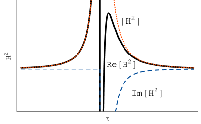
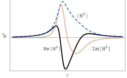
Figure 7: The physical Hubble parameter in radiation era $(\epsilon=2)$ as a function of proper time $\tau$ for different initial conditions. 7 The physical Hubble parameter for observers with real initial condition $U$ defined in Eq. (103) becomes singular at some time $\tau$, which corresponds to the Big Bing singularity. 7 When $U$ in Eq. (103) is complex, the physical Hubble parameter remains finite at all times, thus resolving the Big Bang singularity. The Hubble parameter is in general nonsymmetric under time reversal. Only when $U$ is purely imaginary, the physical Hubble parameter is symmetric under time reversal.

When $U=(u^{0})^{2}_{0}-1=\|\vec{u}\,\|^{2}_{0}$ is complex however, then – as can be seen in figure 7 – both $\Re[H^{2}]$ and $\Im[H^{2}]$ are in general nonzero, implying that the physical Hubble parameter remains finite at all times. We conclude that, just like in the case of curvature domination, there is no curvature singularity except for a set of initial conditions of measure zero ($\Im[u^{0}_{0}]=0$), when compared to the set of all initial conditions ($\Im[u^{0}_{0}]$ arbitrary). The Big Bang singularity is hence resolved also in the radiation era. We think that an analogous conclusion holds for more general expanding space-times. Even though the physics of radiation era is quite different from that of Schwarzschild black holes, the corresponding geodesic equations (64) and (103) – based on which we performed the analyses of singularities – are of an identical form, and thus the conclusions of the analyses are quite similar.

IX Conclusions

We have shown that – just like Hermitian gravity MantzHermitianGravity – holomorphic gravity also resolves the cosmological Big Bang singularity.

Furthermore, we have shown that holomorphic gravity resolves the Schwarzschild space-time singularity. Given the similarities between the Hermitian and holomorphic gravity theories, we expect that Hermitian gravity also does not suffer from the singularity problems of general relativity MantzProkopec:2008 .

Even though, strictly speaking, singularities in complex theories of gravity exist, they occupy just one point on an 8 dimensional phase space, and consequently they are reached only by special geodesics/observers. Indeed, we have argued that the space of initial conditions of observers which encounter singularities is of measure zero, when compared to the space of all initial conditions. Hence quite generically observers will not see singularities within holomorphic gravity. We expect that quantization of space-time and momentum-energy will lead to further smearing of these singularities.

References

- (1) C. L. M. Mantz and T. Prokopec, “Hermitian Gravity and Cosmology,” arXiv:gr-qc/0804.0213
- (2) S. G. Low, “Reciprocal relativity of noninertial frames: quantum mechanics,” J. Phys. A: Math. Theor. 40 (2007) 3999-4016 [arXiv:math-ph/0606015].
- (3) C. L. M. Mantz, “Holomorphic Gravity,” Utrecht University Master’s Thesis (2007) http://www1.phys.uu.nl/ wwwitf/Teaching/2007/Mantz.pdf
- (4) S. W. Hawking and G. F. R. Ellis, “The Large scale structure of space-time,” Cambridge University Press, Cambridge, 1973.
- (5) R. M. Wald, “General Relativity,” Chicago, Usa: Univ. Pr. ( 1984) 491p.
- (6) B. Ratra and P. J. E. Peebles, “Cosmological Consequences of a Rolling Homogeneous Scalar Field,” Phys. Rev. D 37 (1988) 3406. M. Joyce and T. Prokopec, “Turning around the sphaleron bound: Electroweak baryogenesis in an alternative post-inflationary cosmology,” Phys. Rev. D 57 (1998) 6022 [arXiv:hep-ph/9709320].
- (7) C. L. M. Mantz and T. Prokopec, in progress.