Pairing within the self-consistent quasiparticle random-phase approximation at finite temperature

Abstract

An approach to pairing in finite nuclei at nonzero temperature is proposed, which incorporates the effects due to the quasiparticle-number fluctuation (QNF) around Bardeen-Cooper-Schrieffer (BCS) mean field and dynamic coupling to quasiparticle-pair vibrations within the self-consistent quasiparticle random-phase approximation (SCQRPA). The numerical calculations of pairing gap, total energy, and heat capacity were carried out within a doubly folded multilevel model as well as realistic nuclei ⁵⁶Fe and ¹²⁰Sn. The results obtained show that, under the effect of QNF, in the region of moderate and strong couplings, the sharp transition between the superconducting and normal phases is smoothed out, resulting in a thermal pairing gap, which does not collapse at the BCS critical temperature, but has a tail, which extends to high temperature. The dynamic coupling of quasiparticles to SCQRPA vibrations significantly improves the agreement with the results of exact calculations and those obtained within the finite-temperature quantal Monte Carlo method for the total energy and heat capacity. It also causes a deviation of the quasiparticle occupation numbers from the Fermi-Dirac distributions for free fermions.

I INTRODUCTION

Pairing phenomenon is a common feature in strongly interacting many-body systems ranging from tiny ones such as atomic nuclei to very large ones such as neutron stars. Because of its simplicity, the Bardeen-Cooper-Schrieffer (BCS) theory bcs , which explains the conventional superconductivity, has been widely employed as the first step in nuclear structure calculations that include pairing forces. In infinite systems such as low-temperature superconductors, the BCS theory offers a correct description of the pairing gap as functions of temperature $T$ and pairing-interaction strength $G$. Here, as $T$ increases, the BCS gap decreases from its value $\Delta(0)$ at $T=$ 0 until it collapses at a critical temperature $T_{\rm c}=$ 0.567$\Delta(0)$, at which the phase transition between the superconducting phase and normal one (SN-phase transition) occurs es ; Landau . However, the application of the BCS theory to small systems such as atomic nuclei needs to be carried out with a certain care since quantal and thermal fluctuations are not negligible in finite systems, especially when the number of particles is small.

The effects of thermal fluctuations on the pairing properties of nuclei have been the subject of numerous theoretical studies in the last three decades. In the seventies, by applying the macroscopic Landau theory of phase transitions to a uniform model, Moretto has shown that thermal fluctuations smooth out the sharp SN phase transition in finite systems Moretto . In the eighties, this approach was incorporated by Goodman into the Hartree-Fock-Bogoliubov (HFB) theory at finite temperature Goodman1 to account for the effect of thermal fluctuations Goodman2 . Theoretical studies within the static-path approximation (SPA) carried out in the nineties also came to the non-vanishing pairing correlations at finite temperature SPA , which are qualitatively similar to the predictions by Landau theory of phase transitions. The shell-model and Monte-Carlo shell-model calculations shell ; Monte also show that pairing does not abruptly vanish at $T_{\rm c}$, but still survives at $T>T_{\rm c}$. For rotating systems, Frauendorf and collaborators have recently shown a phenomenon of pairing induced by temperature Frau , which reflects strong fluctuations of the order parameter in very small systems with a fixed number of particles. The recent microscopic approach to thermal pairing, called modified-HFB (MHFB) theory MHFB , includes the quasiparticle-number fluctuation (QNF) in the modified single-particle density matrix and particle-pairing tensor. Its limit of constant pairing interaction $G$ is the modified BCS (MBCS) theory MBCS1 ; MBCS2 ; MBCS3 ; MBCS4 . The MBCS theory predicts a pairing gap, which does not collapse at $T_{\rm c}$, but monotonously decreases with increasing $T$, in qualitative agreement with the predictions by the Landau theory of phase transitions and SPA. This feature also agrees with the results obtained by averaging the exact eigenvalues of the pairing problem over the canonical ensemble with a temperature-dependent partition function MBCS3 . The recent extraction of pairing gap from the experimental level densities exp confirms that the pairing gap does not vanish at $T_{\rm c}$ but decreases as $T$ increases, in line with the predictions by these approaches.

The above mentioned approaches are based on the independent quasiparticles, whose occupation numbers follow the Fermi-Dirac distribution of free fermions. Dynamic effects such as those due to coupling to small-amplitude vibrations within the random-phase approximation (RPA) are ignored. These effects have recently been explored by extending the self-consistent particle-particle RPA (SCRPA) to finite temperature using the double-time Green’s function method DaTa . Since the SCRPA fails in the region of strong pairing, where it should be replaced by the quasiparticle representation, it is highly desirable to develop a self-consistent quasiparticle RPA (SCQRPA) at finite temperature, which is workable with any value of pairing interaction parameter $G$.

Recently, we have developed in Ref. SCQRPA a SCQRPA for the multilevel pairing Hamiltonian and applied it to the Richardson model Ric at zero temperature. The derivation of the SCQRPA is based on a set of renormalized BCS equations, which include the corrections due to the QNF and the SCQRPA. The latter arise from the expectation values $\langle{\cal A}^{\dagger}_{j}{\cal A}^{\dagger}_{j^{\prime}}\rangle$ and $\langle{\cal A}^{\dagger}_{j}{\cal A}_{j^{\prime}}\rangle$ in the correlated ground state. Here ${\cal A}^{\dagger}_{j}$ is the product of two time-reversal conjugated quasiparticle operators, $\alpha^{\dagger}_{j}$ and $\alpha^{\dagger}_{-j}$, corresponding to the $j$-th orbital. Within the particle-particle ($pp$) SCRPA SCRPA , these expectation values overscreen the attractive pairing interaction, turning it into repulsion in agreement with the trend of the exact solutions of the Richardson model. For this reason, the expectation values $\langle{\cal A}^{\dagger}_{j}{\cal A}^{\dagger}_{j^{\prime}}\rangle$ and $\langle{\cal A}^{\dagger}_{j}{\cal A}_{j^{\prime}}\rangle$ are called the screening factors. The goal of the present study is to extend the SCQRPA in Ref. SCQRPA to non-zero temperature to explore the effects due to QNF as well as coupling to QRPA vibrations on the pairing properties of finite systems in a self-consistent way.

The article is organized as follows. The derivation of the equations for quasiparticle propagation, which include the effects of QNF and SCQRPA corrections as well as coupling of quasiparticles to pair vibrations at finite temperature is presented Section II. Two approximation schemes will be considered, which are based on the thermal quasiparticle representation without and including dynamic coupling to SCQRPA quasiparticle-pair vibrations. In Section III, the developed approach undergoes a thorough numerical test within the Richardson model as well as in realistic nuclei ⁵⁶Fe and ¹²⁰Sn. The last section summarizes the article, where conclusions are drawn.

II FORMALISM

II.1 Quasiparticle Hamiltonian

The pairing Hamiltonian

$$H=\sum_{jm}\epsilon_{j}a_{jm}^{\dagger}a_{jm}-G\sum_{jj^{\prime}}\sum_{mm^{\prime}>0}a_{jm}^{\dagger}a_{j\widetilde{m}}^{\dagger}a_{j^{\prime}\widetilde{m^{\prime}}}a_{j^{\prime}m^{\prime}}~{}.$$ (1)

describes a set of $N$ particles with single-particle energies $\epsilon_{j}$, which are generated by particle creation operators $a_{jm}^{\dagger}$ on $j$-th orbitals with shell degeneracies $2\Omega_{j}$ ($\Omega_{j}=j+1/2$), and interacting via a monopole-pairing force with a constant parameter $G$. The symbol $~{}~{}\widetilde{}~{}~{}$ denotes the time-reversal operator, namely $a_{j\widetilde{m}}=(-)^{j-m}a_{j-m}$. In general, for a two-component system with $Z$ protons and $N$ neutrons, the sums in Eq. (1) run over all $j_{\tau}m_{\tau}$, $j^{\prime}_{\tau}m^{\prime}_{\tau}$, and $G_{\tau}$ with $\tau=(Z,N)$. This general notation is omitted here as the calculations in the present article are carried out only for one type of particles.

By using the Bogoliubov’s transformation from the particle operators, $a_{jm}^{\dagger}$ and $a_{jm}$, to the quasiparticle ones, $\alpha_{jm}^{\dagger}$ and $\alpha_{jm}$,

$$a_{jm}^{\dagger}=u_{j}\alpha_{jm}^{\dagger}+v_{j}\alpha_{j\widetilde{m}}~{},\hskip 14.22636pta_{j\widetilde{m}}=u_{j}\alpha_{j\widetilde{m}}-v_{j}\alpha_{jm}^{\dagger}~{},$$ (2)

the pairing Hamiltonian (1) is transformed into the quasiparticle Hamiltonian as follows MBCS2 ; MBCS3

$$H=a+\sum_{j}{b_{j}\mathcal{N}_{j}}+\sum_{j}{c_{j}(\mathcal{A}_{j}^{\dagger}+\mathcal{A}_{j}})+\sum_{jj^{\prime}}{d_{jj^{\prime}}\mathcal{A}_{j}^{\dagger}\mathcal{A}_{j^{\prime}}}+\sum_{jj^{\prime}}{g_{j}(j^{\prime})(\mathcal{A}_{j^{\prime}}^{\dagger}\mathcal{N}_{j}+\mathcal{N}_{j}\mathcal{A}_{j^{\prime}})}$$

$$+\sum_{jj^{\prime}}{h_{jj^{\prime}}(\mathcal{A}_{j}^{\dagger}\mathcal{A}_{j^{\prime}}^{\dagger}+\mathcal{A}_{j^{\prime}}\mathcal{A}_{j})}+\sum_{jj^{\prime}}{q_{jj^{\prime}}\mathcal{N}_{j}\mathcal{N}_{j^{\prime}}}~{},$$ (3)

where $\mathcal{N}_{j}$ is the quasiparticle-number operator, whereas $\mathcal{A}_{j}^{\dagger}$ and $\mathcal{A}_{j}$ are the creation and destruction operators of a pair of time-reversal conjugated quasiparticles:

$$\mathcal{N}_{j}=\sum_{m=-\Omega_{j}}^{\Omega_{j}}\alpha_{jm}^{\dagger}\alpha_{jm}=\sum_{m=1}^{\Omega_{j}}(\alpha_{jm}^{\dagger}\alpha_{jm}+\alpha_{j-m}^{\dagger}\alpha_{j-m})~{},$$ (4)

$$\mathcal{A}_{j}^{\dagger}=\frac{1}{\sqrt{2}}\big{[}\alpha^{\dagger}_{j}\otimes\alpha_{j}^{\dagger}\big{]}_{0}^{0}=\frac{1}{\sqrt{\Omega_{j}}}\sum_{m=1}^{\Omega_{j}}\alpha_{jm}^{\dagger}\alpha_{j\widetilde{m}}^{\dagger}~{},\hskip 14.22636pt\mathcal{A}_{j}=(\mathcal{A}_{j}^{\dagger})^{\dagger}~{}.$$ (5)

They obey the following commutation relations

$$[\mathcal{A}_{j}~{},~{}\mathcal{A}_{j^{\prime}}^{\dagger}]=\delta_{jj^{\prime}}{\cal D}_{j}~{},\hskip 5.69054pt{\rm where}\hskip 5.69054pt{\cal D}_{j}=1-\frac{\mathcal{N}_{j}}{\Omega_{j}}~{},$$ (6)

$$[\mathcal{N}_{j}~{},~{}\mathcal{A}_{j^{\prime}}^{\dagger}]=2\delta_{jj^{\prime}}\mathcal{A}_{j^{\prime}}^{\dagger}~{},\hskip 14.22636pt[\mathcal{N}_{j}~{},~{}\mathcal{A}_{j^{\prime}}]=-2\delta_{jj^{\prime}}\mathcal{A}_{j^{\prime}}~{}.$$ (7)

The functionals $a$, $b_{j}$, $c_{j}$, $d_{jj^{\prime}}$, $g_{j}(j^{\prime})$, $h_{jj^{\prime}}$, $q_{jj^{\prime}}$ in Eq. (3) are given in terms of the coefficients $u_{j}$, $v_{j}$ of the Bogoliubov’s transformation, and the single particle energies $\epsilon_{j}$ as (See Eqs. (7) – (13) of Ref. MBCS2 , e.g.)

$$a=2\sum_{j}\Omega_{j}\epsilon_{j}v_{j}^{2}-G\big{(}\sum_{j}\Omega_{j}u_{j}v_{j}\big{)}^{2}-G\sum_{j}\Omega_{j}v_{j}^{4}~{},$$ (8)

$$b_{j}=\epsilon_{j}(u_{j}^{2}-v_{j}^{2})+2Gu_{j}v_{j}\sum_{j^{\prime}}\Omega_{j^{\prime}}u_{j^{\prime}}v_{j^{\prime}}+Gv_{j}^{4}~{},$$ (9)

$$c_{j}=2\sqrt{\Omega_{j}}\epsilon_{j}u_{j}v_{j}-G\sqrt{\Omega_{j}}(u_{j}^{2}-v_{j}^{2})\sum_{j^{\prime}}\Omega_{j^{\prime}}u_{j^{\prime}}v_{j^{\prime}}-2G\sqrt{\Omega_{j}}u_{j}v_{j}^{3}~{},$$ (10)

$$d_{jj^{\prime}}=-G\sqrt{\Omega_{j}\Omega_{j^{\prime}}}(u_{j}^{2}u_{j^{\prime}}^{2}+v_{j}^{2}v_{j^{\prime}}^{2})=d_{j^{\prime}j}~{},$$ (11)

$$g_{j}(j^{\prime})=Gu_{j}v_{j}\sqrt{\Omega_{j^{\prime}}}(u_{j^{\prime}}^{2}-v_{j^{\prime}}^{2})~{},$$ (12)

$$h_{jj^{\prime}}=\frac{G}{2}\sqrt{\Omega_{j}\Omega_{j^{\prime}}}(u_{j}^{2}v_{j^{\prime}}^{2}+v_{j}^{2}u_{j^{\prime}}^{2})=h_{j^{\prime}j}~{},$$ (13)

$$q_{jj^{\prime}}=-Gu_{j}v_{j}u_{j^{\prime}}v_{j^{\prime}}=q_{j^{\prime}j}~{}.$$ (14)

By setting $\Omega_{j}=$ 1 in Eqs. (8) – (14), one recovers the expressions for the case with $\Omega$ doubly-folded levels of the Richardson model (See, e.g., Eqs. (12) – (18) of Ref. SCQRPA ).

II.2 Gap and number equations

The derivation of the equation for the pairing gap that include the effect of correlations in the ground state has been presented briefly in Ref. SCQRPA for the Richardson model. For the clarity of the extension to finite temperature $T$, we give below the detailed derivation of the gap equation, which is applied to the more general quasiparticle Hamiltonian (3) and valid for $T\neq$ 0.

The coefficients $u_{j}$ and $v_{j}$ of the Bogoliubov’s transformation (2) are determined by using the variational procedure, which minimizes the expectation value of the Hamiltonian ${\cal H}=H-\lambda\hat{N}$ in the grand canonical ensemble. This leads to the variational equations Schuck

$$\frac{\partial{\langle{\cal H}\rangle}}{\partial{u_{j}}}+\frac{\partial{\langle{\cal H}\rangle}}{\partial{v_{j}}}\frac{\partial{v_{j}}}{\partial{u_{j}}}\equiv\langle[{\cal H},{\cal A}_{j}^{\dagger}]\rangle=0~{},$$ (15)

where $\langle\hat{\cal O}\rangle$ denotes the ensemble average of the operator $\hat{\cal O}$,

$$\langle\hat{\cal O}\rangle\equiv\frac{{\rm Tr}[\hat{\cal O}e^{-\beta{\cal H}}]}{{\rm Tr}e^{-\beta{\cal H}}}~{},\hskip 28.45274pt\beta=T^{-1}~{}.$$ (16)

The commutation relation $[{\cal H},{\cal A}_{j}^{\dagger}]$ is found by using Eqs. (6) and (7) as

$$[{\cal H},{\cal A}_{j}^{\dagger}]=2b_{j}^{\prime}{\cal A}_{j}^{\dagger}+\bigg{\{}c_{j}^{\prime}+\sum_{j^{\prime}}\big{[}d_{jj^{\prime}}{\cal A}_{j^{\prime}}^{\dagger}+g_{j^{\prime}}(j){\cal N}_{j^{\prime}}+h_{jj^{\prime}}{\cal A}_{j^{\prime}}\big{]}\bigg{\}}{\cal D}_{j}$$

$$+2\sum_{j^{\prime}}\bigg{\{}g_{j}(j^{\prime})\big{[}{\cal A}^{\dagger}_{j^{\prime}}{\cal A}^{\dagger}_{j}+{\cal A}^{\dagger}_{j}{\cal A}_{j^{\prime}}\big{]}+q_{jj^{\prime}}\big{[}{\cal A}^{\dagger}_{j}{\cal N}_{j^{\prime}}+{\cal N}_{j^{\prime}}{\cal A}^{\dagger}_{j}\big{]}\bigg{\}}+\sum_{j^{\prime}}h_{jj^{\prime}}{\cal D}_{j}{\cal A}_{j^{\prime}}~{}.$$ (17)

The ensemble average of the commutation relation (17) is then given as

$$\langle[{\cal H},{\cal A}_{j}^{\dagger}]\rangle=c_{j}^{\prime}\langle{\cal D}_{j}\rangle+\sum_{j^{\prime}}\bigg{\{}2g_{j}(j^{\prime})\big{[}\langle{\cal A}^{\dagger}_{j^{\prime}}{\cal A}^{\dagger}_{j}\rangle+\langle{\cal A}^{\dagger}_{j}{\cal A}_{j^{\prime}}\rangle\big{]}+g_{j^{\prime}}(j)\langle{\cal N}_{j^{\prime}}{\cal D}_{j}\rangle\bigg{\}}~{},$$ (18)

where the functionals $b_{j}^{\prime}$ and $c_{j}^{\prime}$ are

$$b_{j}^{\prime}=b_{j}-\lambda(u_{j}^{2}-v_{j}^{2})~{},\hskip 14.22636ptc_{j}^{\prime}=c_{j}-2\lambda\sqrt{\Omega_{j}}u_{j}v_{j}~{},$$ (19)

i.e. they have the same form as that of $b_{j}$ in Eq. (9), and $c_{j}$ in Eq. (10), but with $\epsilon_{j}-\lambda$ replacing $\epsilon_{j}$ at the right-hand sides. Inserting the explicit expressions for the functionals $c_{j}^{\prime}$ from Eq. (19) as well as $g_{j}(j^{\prime})$ and $g_{j^{\prime}}(j)$ from Eq. (12) into the right-hand side of Eq. (18), and equalizing the obtained result to zero as required by the variational procedure (15), we come to the following equation, which is formally identical to the BCS one:

$$2(\epsilon^{\prime}_{j}-Gv_{j}^{2}-\lambda)u_{j}v_{j}-\Delta_{j}(u_{j}^{2}-v_{j}^{2})=0~{},$$ (20)

where, however, the single-particle energies $\epsilon^{\prime}_{j}$ are renormalized as

$$\epsilon_{j}^{\prime}=\epsilon_{j}+\frac{G}{\sqrt{\Omega_{j}}\langle{\cal D}_{j}\rangle}\sum_{j^{\prime}}\sqrt{\Omega_{j^{\prime}}}(u_{j^{\prime}}^{2}-v_{j^{\prime}}^{2})\bigg{(}\langle{\cal A}_{j}^{\dagger}{\cal A}_{j^{\prime}}^{\dagger}\rangle+\langle{\cal A}_{j}^{\dagger}{\cal A}_{j^{\prime}}\rangle\bigg{)}~{}.$$ (21)

The pairing gap is found as the solution of the following equation

$$\Delta_{j}=\frac{G}{\langle{\cal D}_{j}\rangle}{\sum_{j^{\prime}}\Omega_{j^{\prime}}\langle{\cal D}_{j}{\cal D}_{j^{\prime}}\rangle}u_{j^{\prime}}v_{j^{\prime}}~{},$$ (22)

which is level-dependent. The coefficients $u_{j}$ and $v_{j}$ of the Bogoliubov’s transformation (2) are derived in a standard way from Eq. (20) and the unitarity constraint $u_{j}^{2}+v_{j}^{2}=$ 1. They read

$$u_{j}^{2}=\frac{1}{2}\bigg{(}1+\frac{\epsilon^{\prime}_{j}-Gv_{j}^{2}-\lambda}{E_{j}}\bigg{)}~{},\hskip 14.22636ptv_{j}^{2}=\frac{1}{2}\bigg{(}1-\frac{\epsilon^{\prime}_{j}-Gv_{j}^{2}-\lambda}{E_{j}}\bigg{)}~{},$$ (23)

where $E_{j}$ are the quasiparticle energies

$$E_{j}=\sqrt{(\epsilon^{\prime}_{j}-Gv_{j}^{2}-\lambda)^{2}+\Delta_{j}^{2}}~{}.$$ (24)

The particle-number equation is obtained by transforming the particle-number operator $\hat{N}\equiv\sum_{jm}a_{jm}^{\dagger}a_{jm}$ into the quasiparticle presentation using the Bogoliubov’s transformation (2) and taking the ensemble average. The result is

$$N=2\sum_{j}\Omega_{j}\bigg{[}v_{j}^{2}\langle{\cal D}_{j}\rangle+\frac{1}{2}\big{(}1-\langle{\cal D}_{j}\rangle\big{)}\bigg{]}~{}.$$ (25)

The pairing gap $\Delta_{j}$ and chemical potential $\lambda$, which is the Lagrangian multiplier in the variational equations (15), are determined as solutions of Eqs. (22) and (25).

The right-hand side of Eq. (22) contains the expectation values $\langle{\cal D}_{j}{\cal D}_{j^{\prime}}\rangle$, whose exact treatment is not possible as it involves an infinite boson expansion series Samba . In the present article, following the treatment on Ref. SCQRPA , we use the exact relation

$$\langle{\cal D}_{j}{\cal D}_{j^{\prime}}\rangle=\langle{\cal D}_{j}\rangle\langle{\cal D}_{j^{\prime}}\rangle+\frac{\delta{\cal N}_{jj^{\prime}}}{\Omega_{j}\Omega_{j^{\prime}}}~{},\hskip 14.22636pt{\rm with}\hskip 14.22636pt\delta{\cal N}_{jj^{\prime}}=\langle{\cal N}_{j}{\cal N}_{j^{\prime}}\rangle-\langle{\cal N}_{j}\rangle\langle{\cal N}_{j^{\prime}}\rangle~{},$$ (26)

and the mean-field contraction for the term $\delta{\cal N}_{jj^{\prime}}$

$$\delta{\cal N}_{jj^{\prime}}\simeq 2\Omega_{j}\delta{\cal N}_{j}^{2}\delta_{jj^{\prime}}~{},\hskip 14.22636pt\delta{\cal N}_{j}^{2}\equiv n_{j}(1-n_{j})~{},$$ (27)

with the quasiparticle occupation number $n_{j}$

$$n_{j}=\frac{\langle{\cal N}_{j}\rangle}{2\Omega_{j}}=\frac{1}{2}(1-\langle{\cal D}_{j}\rangle)~{},$$ (28)

to rewrite the gap equation (22) as a sum of a level-independent part, $\Delta$, and a level-dependent part, $\delta\Delta_{j}$, namely

$$\Delta_{j}=\Delta+\delta\Delta_{j}~{},$$ (29)

where

$$\Delta=G\sum_{j^{\prime}}\Omega_{j^{\prime}}\langle{\cal D}_{j^{\prime}}\rangle u_{j^{\prime}}v_{j^{\prime}}~{},\hskip 14.22636pt\delta\Delta_{j}=2G\frac{\delta{\cal N}_{j}^{2}}{\langle{\cal D}_{j}\rangle}u_{j}v_{j}~{}.$$ (30)

The quantity $\delta{\cal N}_{j}^{2}$ in Eqs. (27) and (30), is nothing but the standard expression for the QNF corresponding to the $j$-th orbital Goodman2 ; MHFB . Using Eqs. (23) and (30), after simple algebras, we rewrite the gap (29) in the following form

$$\Delta_{j}=\frac{\widetilde{G}_{j}}{2}\sum_{j^{\prime}}\Omega_{j^{\prime}}\langle{\cal D}_{j^{\prime}}\rangle\frac{\Delta_{j^{\prime}}}{E_{j^{\prime}}}~{},\hskip 14.22636pt{\rm where}\hskip 14.22636pt\widetilde{G}_{j}={G}\bigg{(}1-G\frac{\delta{\cal N}_{j}^{2}}{\langle{\cal D}_{j}\rangle E_{j}}\bigg{)}^{-1}~{}.$$ (31)

II.3 Finite-temperature BCS with quasiparticle number fluctuations

II.3.1 Without particle-number projection (FTBCS1)

The gap equation (31) is remarkable as it shows that the QNF $\delta{\cal N}_{j}^{2}$ renormalizes the pairing interaction $G$ to $\widetilde{G}_{j}$. The conventional finite-temperature BCS (FTBCS) gap equation $\Delta_{j}=\Delta$ is recovered from Eq. (31) when the following assumptions simultaneously hold:

i) Independent quasiparticles: $n_{j}=n_{j}^{\rm FD}$, where $n_{j}^{\rm FD}$ is the Fermi-Dirac distribution of non-interacting fermions

$$n_{j}^{\rm FD}=\frac{1}{e^{\beta E_{j}}+1}~{},$$ (32)

ii) No quasiparticle number fluctuation: $\delta{\cal N}^{2}_{j}=$ 0 ,

iii) No screening factors: $\langle{\cal A}_{j}^{\dagger}{\cal A}_{j^{\prime}}^{\dagger}\rangle=\langle{\cal A}_{j}^{\dagger}{\cal A}_{j^{\prime}}\rangle=$ 0  in Eq. (21).

These three assumptions guaranty a thermal quasiparticle mean field, in which quasiparticles are moving independently without any perturbation caused by the QNF and/or coupling to multiple quasiparticle configurations beyond the quasiparticle mean field. Among these configurations, the simplest ones are the small-amplitude vibrations (QRPA corrections). From these assumptions, one can infer that releasing assumption ii) allows us to include the effect of QNF, provided the quantal effect of coupling to QRPA vibrations is negligible, i.e. assumption iii) still holds. In the present article, this approximation scheme, for which i) and iii) hold, whereas $\delta{\cal N}_{j}^{2}\neq$ 0, is referred to as the FTBCS1.

II.3.2 With Lipkin-Nogami particle-number projection (FTLN1)

The problem of particle-number violation within the BCS theory is usually resolved in the simplest way by means of an approximated particle-number projection (PNP) before variation called the Lipkin-Nogami (LN) method LN . In Ref. SCQRPA this method has been applied to the BCS1 and the resulting approach is called the LN1. For the case with $\Omega_{j}\neq$ 1 and level-dependent gap $\Delta_{j}$ (29) at $T\neq$ 0, the corresponding finite-temperature LN1 equations have the form

$$\tilde{\Delta}_{j}=G\sum_{j^{\prime}}\Omega_{j^{\prime}}\tilde{\tau}_{jj^{\prime}}~{},\hskip 8.53581ptN=2\sum_{j}\Omega_{j}\tilde{\rho}_{j}~{},\hskip 14.22636pt\tilde{\epsilon}_{j}=\epsilon^{\prime}_{j}+(4\lambda_{2}-G){\tilde{v}_{j}}^{2}~{},\hskip 8.53581pt\lambda=\lambda_{1}+2\lambda_{2}(N+1)~{},$$ (33)

where

$$\tilde{\tau}_{jj^{\prime}}=\tau_{jj^{\prime}}+\frac{2}{\Omega_{j}}\frac{\delta{\cal N}_{j}^{2}}{\langle{\cal D}_{j}\rangle}\delta_{jj^{\prime}}\tilde{u}_{j^{\prime}}\tilde{v}_{j^{\prime}}~{},\hskip 14.22636pt\tau_{jj^{\prime}}=\langle{\cal D}_{j^{\prime}}\rangle\tilde{u}_{j^{\prime}}\tilde{v}_{j^{\prime}}~{},\hskip 14.22636pt\tilde{\rho}_{j}=\tilde{v}_{j}^{2}\langle{\cal D}_{j}\rangle+\frac{1}{2}(1-\langle{\cal D}_{j}\rangle)~{},$$ (34)

$$\tilde{u}_{j}^{2}=\frac{1}{2}\left(1+\frac{\tilde{\epsilon}_{j}-\lambda}{\tilde{E}_{j}}\right)~{},\hskip 14.22636pt\tilde{v}_{j}^{2}=\frac{1}{2}\left(1-\frac{\tilde{\epsilon}_{j}-\lambda}{\tilde{E}_{j}}\right)~{},\hskip 14.22636pt\tilde{E}_{j}=\sqrt{(\tilde{\epsilon}_{j}-\lambda)^{2}+\tilde{\Delta}_{j}^{2}}~{}.$$ (35)

The coefficient $\lambda_{2}$ is given as SCQRPA

$$\lambda_{2}=\frac{G}{4}\frac{\sum_{j}\Omega_{j}(1-\tilde{\rho}_{j})\tau_{j}\sum_{j^{\prime}}\Omega_{j^{\prime}}\tilde{\rho}_{j^{\prime}}\tau_{j^{\prime}}-\sum_{j}\Omega_{j}(1-\tilde{\rho}_{j})^{2}\tilde{\rho}_{j}^{2}}{\left[\sum_{j}\Omega_{j}\tilde{\rho}_{j}(1-\tilde{\rho}_{j})\right]^{2}-\sum_{j}\Omega_{j}(1-\tilde{\rho}_{j})^{2}\tilde{\rho}_{j}^{2}}~{},$$ (36)

where $\tau_{j}\equiv\tau_{jj}$. This FTBCS1 including the approximated PNP within the LN method is referred to as FTLN1 in the present article. It is worth pointing out that, being an approximated projection that corrects for the quantal fluctuations of particle number within the BCS theory, the LN method in the present formulation is not sufficient to account for the thermal fluctuations (QNF) around the phase transition point $T\sim T_{\rm c}$ as well as at high $T$. Another well-known defect of the LN method is that it produces a large pairing gap (pairing correlation energy) even in closed-shell nuclei, where there should be no pairing gap. The source of this pathological behavior is assigned to the fast change of $\lambda_{2}$ at the shell closure, which invalidates the truncation of the expansion at second order patho . In Ref. MBCS4 , it has been demonstrated within the MBCS theory that the projection-after-variation (PAV) method offers much better results, which are closer to the exact solutions. The PAV at $T\neq$ 0, however, is much more complicated than the LN method. Therefore, we prefer to devote a separate study to its application to the BCS1.

II.4 Finite-temperature BCS with quasiparticle-number fluctuation and dynamic coupling to SCQRPA vibrations (FTBCS1+SCQRPA and FTLN1+SCQRPA)

As has been mentioned in the preceding section, within the quasiparticle mean field, the expectation values $\langle{\cal A}_{j}^{\dagger}{\cal A}_{j^{\prime}}^{\dagger}\rangle$ and $\langle{\cal A}_{j}^{\dagger}{\cal A}_{j^{\prime}}\rangle$ at the right-hand side of Eq. (21) are always zero [Assumption iii)]. They cannot be factorized into the products of expectation values of quasiparticle-number operators within the thermal quasiparticle mean field because such crude contraction is tantamount to artificially breaking the pair correlators (5) (See the Appendix A). Therefore, to account for the correlations beyond the quasiparticle mean field, these screening factors should be estimated, at least, within the SCQRPA, where they can be expressed below in terms of the forward- and backward going amplitudes, ${\cal X}^{\mu}_{j}$ and ${\cal Y}^{\mu}_{j}$, of the SCQRPA operators (phonons) as SCQRPA

$${\cal Q}_{\mu}^{\dagger}=\sum_{j}\bigg{(}\frac{{\cal X}_{j}^{\mu}}{\sqrt{\langle{\cal D}_{j}\rangle}}{\cal A}_{j}^{\dagger}-\frac{{\cal Y}_{j}^{\mu}}{\sqrt{\langle{\cal D}_{j}\rangle}}{\cal A}_{j}\bigg{)}~{},\hskip 14.22636pt{\cal Q}_{\mu}=[{\cal Q}_{\mu}^{\dagger}]^{\dagger}~{}.$$ (37)

The renormalization factor $\sqrt{\langle{\cal D}_{j}\rangle}$ is introduced in Eq. (37) to ensure that the SCQRPA operators ${\cal Q}_{\mu}^{\dagger}$ and ${\cal Q}_{\mu}$ remain bosons within the thermal average (16), preserving the exact commutation relation (6). This leads to the orthogonality relation for the ${\cal X}_{j}^{\mu}$ and ${\cal Y}_{j}^{\mu}$ amplitudes in the conventional form as

$$\sum_{j}\big{(}{\cal X}_{j}^{\mu}{\cal X}_{j}^{\mu^{\prime}}-{\cal Y}_{j}^{\mu}{\cal Y}_{j}^{\mu^{\prime}}\big{)}=\delta_{\mu\mu^{\prime}}~{},$$ (38)

which can be easily verified by calculating $\langle[{\cal Q}_{\mu},{\cal Q}_{\mu^{\prime}}^{\dagger}]\rangle$ and requiring that the result to be equal to $\delta_{\mu\mu^{\prime}}$. The inverse transformation of Eq. (37) reads

$${\cal A}_{j}^{\dagger}=\sqrt{\langle{\cal D}_{j}}\rangle\sum_{\mu}\big{(}{\cal X}_{j}^{\mu}{\cal Q}_{\mu}^{\dagger}+{\cal Y}_{j}^{\mu}{\cal Q}_{\mu}\big{)}~{},$$ (39)

provided the following conventional closure relations hold

$$\sum_{\mu}\big{(}{\cal X}_{j}^{\mu}{\cal X}_{j^{\prime}}^{\mu}-{\cal Y}_{j}^{\mu}{\cal Y}_{j^{\prime}}^{\mu}\big{)}=\delta_{jj^{\prime}}~{},\hskip 14.22636pt\sum_{\mu}\big{(}{\cal X}_{j}^{\mu}{\cal Y}_{j^{\prime}}^{\mu}-{\cal Y}_{j}^{\mu}{\cal X}_{j^{\prime}}^{\mu}\big{)}=0~{},$$ (40)

II.4.1 Screening factors

Using the inverse transformation (39), we obtain the expectation values $\langle{\cal A}_{j}^{\dagger}{\cal A}_{j^{\prime}}^{\dagger}\rangle$ and $\langle{\cal A}_{j}^{\dagger}{\cal A}_{j^{\prime}}\rangle$ at $T\neq$ 0 in the form

$$x_{jj^{\prime}}\equiv\frac{\langle{\cal A}_{j}^{\dagger}{\cal A}_{j^{\prime}}\rangle}{\sqrt{\langle{\cal D}_{j}\rangle\langle{\cal D}_{j^{\prime}}\rangle}}=\sum_{\mu}{\cal Y}_{j}^{\mu}{\cal Y}_{j^{\prime}}^{\mu}+\sum_{\mu\mu^{\prime}}\bigg{(}U_{jj^{\prime}}^{\mu\mu^{\prime}}\langle{\cal Q}^{\dagger}_{\mu}{\cal Q}_{\mu^{\prime}}\rangle+Z_{jj^{\prime}}^{\mu\mu^{\prime}}\langle{\cal Q}^{\dagger}_{\mu}{\cal Q}_{\mu^{\prime}}^{\dagger}\rangle\bigg{)}~{},$$ (41)

$$y_{jj^{\prime}}\equiv\frac{\langle{\cal A}_{j}^{\dagger}{\cal A}_{j^{\prime}}^{\dagger}\rangle}{\sqrt{\langle{\cal D}_{j}\rangle\langle{\cal D}_{j^{\prime}}\rangle}}=\sum_{\mu}{\cal Y}_{j}^{\mu}{\cal X}_{j^{\prime}}^{\mu}+\sum_{\mu\mu^{\prime}}\bigg{(}U_{jj^{\prime}}^{\mu\mu^{\prime}}\langle{\cal Q}^{\dagger}_{\mu}{\cal Q}_{\mu^{\prime}}^{\dagger}\rangle+Z_{jj^{\prime}}^{\mu\mu^{\prime}}\langle{\cal Q}^{\dagger}_{\mu}{\cal Q}_{\mu^{\prime}}\rangle\bigg{)}~{},$$ (42)

where the following shorthand notations are used

$${U}_{jj^{\prime}}^{\mu\mu^{\prime}}={\cal X}_{j}^{\mu}{\cal X}_{j^{\prime}}^{\mu^{\prime}}+{\cal Y}_{j^{\prime}}^{\mu}{\cal Y}_{j}^{\mu^{\prime}}~{},\hskip 14.22636pt{Z}_{jj^{\prime}}^{\mu\mu^{\prime}}={\cal X}_{j}^{\mu}{\cal Y}_{j^{\prime}}^{\mu^{\prime}}+{\cal Y}_{j}^{\mu^{\prime}}{\cal X}_{j^{\prime}}^{\mu}~{}.$$ (43)

taking into account the symmetry property $\langle{\cal Q}_{\mu}^{\dagger}{\cal Q}_{\mu^{\prime}}^{\dagger}\rangle=\langle{\cal Q}_{\mu}{\cal Q}_{\mu^{\prime}}\rangle$. Using now the definition (37), we express the expectation values $\langle{\cal Q}_{\mu}^{\dagger}{\cal Q}_{\mu^{\prime}}\rangle$ and $\langle{\cal Q}_{\mu}^{\dagger}{\cal Q}_{\mu^{\prime}}^{\dagger}\rangle$ in terms of $x_{jj^{\prime}}$ (i.e. $\langle{\cal A}^{\dagger}_{j}{\cal A}_{j^{\prime}}\rangle$), $y_{jj^{\prime}}$ (i.e. $\langle{\cal A}^{\dagger}_{j}{\cal A}_{j^{\prime}}^{\dagger}\rangle$), and amplitudes ${\cal X}_{j}^{\mu}$ and ${\cal Y}_{j}^{\mu}$ as

$$\langle{\cal Q}_{\mu}^{\dagger}{\cal Q}_{\mu^{\prime}}\rangle=\sum_{j}{\cal Y}_{j}^{\mu}{\cal Y}_{j}^{\mu^{\prime}}+\sum_{jj^{\prime}}(U_{jj^{\prime}}^{\mu\mu^{\prime}}x_{jj^{\prime}}-W_{jj^{\prime}}^{\mu\mu^{\prime}}y_{jj^{\prime}})~{},$$ (44)

$$\langle{\cal Q}_{\mu}^{\dagger}{\cal Q}_{\mu^{\prime}}^{\dagger}\rangle=-\sum_{j}{\cal Y}_{j}^{\mu}{\cal X}_{j}^{\mu^{\prime}}+\sum_{jj^{\prime}}(U_{jj^{\prime}}^{\mu\mu^{\prime}}y_{jj^{\prime}}-W_{jj^{\prime}}^{\mu\mu^{\prime}}x_{jj^{\prime}})~{},$$ (45)

where

$$W^{\mu\mu^{\prime}}_{jj^{\prime}}={\cal X}_{j}^{\mu}{\cal Y}_{j^{\prime}}^{\mu^{\prime}}+{\cal Y}_{j^{\prime}}^{\mu}{\cal X}_{j}^{\mu^{\prime}}~{}.$$ (46)

Inserting Eqs. (44) and (45) into the right-hand sides of Eqs. (41) and (42), after some simple algebras, we obtain the following set of exact equations for the screening factors (41) and (42)

$$\sum_{j_{1}j^{\prime}_{1}}\bigg{[}\delta_{jj_{1}}\delta_{j^{\prime}j_{1}^{\prime}}-\sum_{\mu\mu^{\prime}}\big{(}U_{jj^{\prime}}^{\mu\mu^{\prime}}U_{j_{1}j_{1}^{\prime}}^{\mu\mu^{\prime}}-Z_{jj^{\prime}}^{\mu\mu^{\prime}}W_{j_{1}j_{1}^{\prime}}^{\mu\mu^{\prime}}\big{)}\bigg{]}x_{j_{1}j_{1}^{\prime}}+\sum_{j_{1}j_{1}^{\prime}\mu\mu^{\prime}}\big{(}U_{jj^{\prime}}^{\mu\mu^{\prime}}W_{j_{1}j_{1}^{\prime}}^{\mu\mu^{\prime}}-Z_{jj^{\prime}}^{\mu\mu^{\prime}}U_{j_{1}j_{1}^{\prime}}^{\mu\mu^{\prime}}\big{)}y_{j_{1}j_{1}^{\prime}}$$

$$=\sum_{\mu}{\cal Y}_{j}^{\mu}{\cal Y}_{j^{\prime}}^{\mu}+\sum_{j^{\prime\prime}\mu\mu^{\prime}}{\cal Y}_{j^{\prime\prime}}^{\mu}\big{(}U_{jj^{\prime}}^{\mu\mu^{\prime}}{\cal Y}_{j^{\prime\prime}}^{\mu^{\prime}}-Z_{jj^{\prime}}^{\mu\mu^{\prime}}{\cal X}_{j^{\prime\prime}}^{\mu^{\prime}}\big{)}~{},$$ (47)

$$\sum_{j_{1}j_{1}^{\prime}\mu\mu^{\prime}}\big{(}U_{jj^{\prime}}^{\mu\mu^{\prime}}W_{j_{1}j_{1}^{\prime}}^{\mu\mu^{\prime}}-Z_{jj^{\prime}}^{\mu\mu^{\prime}}U_{j_{1}j_{1}^{\prime}}^{\mu\mu^{\prime}}\big{)}x_{j_{1}j_{1}^{\prime}}+\sum_{j_{1}j^{\prime}_{1}}\bigg{[}\delta_{jj_{1}}\delta_{j^{\prime}j_{1}^{\prime}}-\sum_{\mu\mu^{\prime}}\big{(}U_{jj^{\prime}}^{\mu\mu^{\prime}}U_{j_{1}j_{1}^{\prime}}^{\mu\mu^{\prime}}-Z_{jj^{\prime}}^{\mu\mu^{\prime}}W_{j_{1}j_{1}^{\prime}}^{\mu\mu^{\prime}}\big{)}\bigg{]}y_{j_{1}j_{1}^{\prime}}$$

$$=\sum_{\mu}{\cal Y}_{j}^{\mu}{\cal X}_{j^{\prime}}^{\mu}+\sum_{j^{\prime\prime}\mu\mu^{\prime}}{\cal Y}_{j^{\prime\prime}}^{\mu}\big{(}Z_{jj^{\prime}}^{\mu\mu^{\prime}}{\cal Y}_{j^{\prime\prime}}^{\mu^{\prime}}-U_{jj^{\prime}}^{\mu\mu^{\prime}}{\cal X}_{j^{\prime\prime}}^{\mu^{\prime}}\big{)}~{}.$$ (48)

The derivation of the SCQRPA equations at finite temperature is proceeded in the same way as has been done at $T=$ 0, and is formally identical to Eqs. (46), (56), and (57) of Ref. SCQRPA so we do not repeat them here. Notice that the expectation values $\langle{\cal D}_{j}{\cal D}_{j^{\prime}}\rangle$ in the submatrices A and B in Eqs. (56) and (57) of Ref. SCQRPA are now calculated by using Eqs. (26) and (27). The approach that solves the number and gap equations (25), (29) – (27), as well as equations for the screening factors (47) and (48) selfconsistently with the SCQRPA ones at $T\neq$ 0, where all the assumptions i) – iii) cease to hold, is called the FTBCS1+SCQRPA in the present article. The corresponding approach that includes also PNP within the LN method is called as FTLN1+SCQRPA.

II.4.2 Quasiparticle occupation number

To complete the set of FTBCS1+SCQRPA equations we still need an equation for the quasiparticle occupation number $n_{j}$ defined in Eq. (28). Here comes the principal difference of the FTBCS1+SCQRPA compared to the zero-temperature SCQRPA since $n_{j}$ should be calculated selfconsistently from the SCQRPA taking into account dynamic coupling between quasiparticles and SCQRPA phonons at $T\neq$ 0 in an infinite hierarchy of algebraic equations. The quasiparticle propagator found as the formal solution of this hierarchy of equations is different from that for free quasiparticles by the mass operator, which reflects the effects of coupling to complex configurations. Since the latter cannot be treated exactly, approximations have to be made to close the hierarchy. Following the same line as in Ref. DaTa , we derive in this section a set of equations for the quasiparticle propagator and quasiparticle occupation number $n_{j}$ at $T\neq$ 0 by using the method of double-time Green’s functions Bogo ; Zubarev . To close the hierarchy of equations, we lower the order of double-time Green’s functions by applying the standard decoupling approximation introduced by Bogoliubov and Tyablikov  Bogo ; Zubarev .

By noticing that the only term in the quasiparticle Hamiltonian (3) that cannot be taken into account within either the BCS theory or the SCQRPA is the sum containing $g_{j}(j^{\prime})$ functionals, we effectively rewrite Hamiltonian ${\cal H}$ in Eq. (15) as

$${\cal H}_{eff}=\sum_{j}(b^{\prime}_{j}+\sum_{j^{\prime}}q_{jj^{\prime}}{\cal N}_{j^{\prime}}){\cal N}_{j}+\sum_{\mu}\omega_{\mu}{\cal Q}_{\mu}^{\dagger}{\cal Q}_{\mu}+\sum_{j\mu}V_{j}^{\mu}{\cal N}_{j}({\cal Q}_{\mu}^{\dagger}+{\cal Q}_{\mu})~{}.$$ (49)

The first sum at the right-hand side of this representation describes the part of the quasiparticle Hamiltonian (3), which cannot be expressed in terms of phonon operators (37). Within the BCS theory, where the part containing $q_{jj^{\prime}}$ does not contribute whereas the term $\sim Gv_{j}^{4}$ and the QNF are neglected, one obtains $b^{\prime}_{j}=E_{j}$. In this case, this sum corresponds to the quasiparticle mean field. The second sum describes the SCQRPA Hamiltonian after solving the SCQRPA equations, which give the amplitudes ${\cal X}_{j}^{\mu}$, ${\cal Y}^{\mu}_{j}$, and the SCQRPA energies $\omega_{\mu}$. The last sum represents the coupling between the quasiparticle and phonon fields, which is left out from the BCS (FTBCS1) and the QRPA (SCQRPA). This sum is rewritten here in terms of ${\cal N}_{j}$ and SCQRPA operators by using the inverse transformation (39). The vertex $V_{j}^{\mu}$ obtained after this transformation has the form

$$V_{j}^{\mu}=\sum_{j^{\prime}}g_{j}(j^{\prime})\sqrt{\langle{\cal D}_{j^{\prime}}\rangle}({\cal X}_{j^{\prime}}^{\mu}+{\cal Y}_{j^{\prime}}^{\mu})~{}.$$ (50)

Given that ${\cal N}_{j}$ commutes with ${\cal Q}^{\dagger}_{\mu}$ within the SCQRPA, such effective representation of the quasiparticle Hamiltonian causes no double counting between the first two sums at the right-hand side of Eq. (49), but becomes convenient for the derivation of the quasiparticle Green’s function, which includes the coupling to SCQRPA modes, because the first sum is activated only in the quasiparticle space, whereas the second sum functions only in the phonon space.

Following closely the procedure described in Section 8.1 of Ref. Zubarev , we introduce the double-time retarded Green’s functions, which describe

a) The quasiparticle propagation:

$$G_{j}(t-t^{\prime})=\langle\langle\alpha_{j}(t);\alpha^{\dagger}_{j}(t^{\prime})\rangle\rangle~{},$$ (51)

b) Quasiparticle-phonon coupling:

$${\Gamma}_{j\mu}^{-}(t-t^{\prime})=\langle\langle\alpha_{j}(t){\cal Q}_{\mu}(t);\alpha^{\dagger}_{j}(t^{\prime})\rangle\rangle~{},\hskip 14.22636pt{\Gamma}_{j\mu}^{+}(t-t^{\prime})=\langle\langle\alpha_{j}(t){\cal Q}_{\mu}^{\dagger}(t);\alpha^{\dagger}_{j}(t^{\prime})\rangle\rangle~{}.$$ (52)

The magnetic quantum number $m$ in $\alpha_{jm}^{\dagger}$ and $\alpha_{jm}$ is omitted hereafter for simplicity as the results below do not depend on $m$. The definitions (51) and (52) use the standard notation $G_{r}(t-t^{\prime})=\langle\langle A(t);B(t^{\prime})\rangle\rangle\equiv-i\theta(t-t^{\prime})\langle[A(t),B(t^{\prime})]\rangle$ for the double-time retarded Green’s function $G_{r}(t-t^{\prime})$ built from operators $A(t)$ at time $t$ and $B(t^{\prime})$ at time $t^{\prime}$. The advantage of using the double-time retarded Green’s function is that this type of Green’s function can be analytically continued into the complex energy plane. The imaginary part of the mass operator in this analytic continuation corresponds to the quasiparticle damping caused by the quasiparticle-phonon coupling. This method is free from any constraints of perturbation theory.

Applying the standard method of deriving the equation of motion for the double-time Green’s function, namely

$$i\frac{\partial G_{r}(t-t^{\prime})}{\partial t}=\delta(t-t^{\prime})\langle[A(t),B(t)]_{\pm}\rangle+\langle\langle[A(t),H(t)];B(t^{\prime})\rangle\rangle~{},$$ (53)

to the Green’s functions (51) and (52) with the effective Hamiltonian (49), we find for them a set of three exact equations

$$i\frac{\partial G_{j}(t-t^{\prime})}{\partial t}=\delta(t-t^{\prime})+\widetilde{E_{j}}G_{j}(t-t^{\prime})+\sum_{\mu}V_{j}^{\mu}\big{[}\Gamma_{j\mu}^{-}(t-t^{\prime})+\Gamma_{j\mu}^{+}(t-t^{\prime})\big{]}~{},$$ (54)

$$i\frac{\partial\Gamma_{j\mu}^{-}(t-t^{\prime})}{\partial t}=(\widetilde{E}_{j}+\omega_{\mu})\Gamma_{j\mu}^{-}(t-t^{\prime})+\sum_{\mu^{\prime}}V_{j}^{\mu^{\prime}}\langle\langle\alpha_{j}(t)\big{[}{\cal Q}_{\mu^{\prime}}^{\dagger}(t)+{\cal Q}_{\mu^{\prime}}(t)\big{]}{\cal Q}_{\mu}(t);\alpha^{\dagger}_{j}(t^{\prime})\rangle\rangle$$

$$+\sum_{j^{\prime}}V_{j^{\prime}}^{\mu}\langle\langle\alpha_{j}(t){\cal N}_{j^{\prime}}(t);\alpha^{\dagger}(t^{\prime})\rangle\rangle~{},$$ (55)

$$i\frac{\partial\Gamma_{j\mu}^{+}(t-t^{\prime})}{\partial t}=(\widetilde{E}_{j}-\omega_{\mu})\Gamma_{j\mu}^{+}(t-t^{\prime})+\sum_{\mu^{\prime}}V_{j}^{\mu^{\prime}}\langle\langle\alpha_{j}(t)\big{[}{\cal Q}_{\mu^{\prime}}^{\dagger}(t)+{\cal Q}_{\mu^{\prime}}(t)\big{]}{\cal Q}_{\mu}^{\dagger}(t);\alpha^{\dagger}_{j}(t^{\prime})\rangle\rangle$$

$$-\sum_{j^{\prime}}V_{j^{\prime}}^{\mu}\langle\langle\alpha_{j}(t){\cal N}_{j^{\prime}}(t);\alpha^{\dagger}(t^{\prime})\rangle\rangle~{},$$ (56)

where

$$\widetilde{E}_{j}=b^{\prime}_{j}+q_{jj}~{}.$$ (57)

The last two equations, Eqs. (55) and (56), from this set contain higher-order Green’s functions, which should be decoupled so that the set can be closed. Following the method proposed by Bogoliubov and Tyablikov Bogo , we decouple the higher-order Green’s functions at the right-hand side of Eqs. (55) and (56) by pairing off operators referring to the same time, namely

$$\langle\langle\alpha_{j}(t)\big{[}{\cal Q}_{\mu^{\prime}}^{\dagger}(t)+{\cal Q}_{\mu^{\prime}}(t)\big{]}{\cal Q}_{\mu}(t);\alpha^{\dagger}_{j}(t^{\prime})\rangle\rangle\simeq\delta_{\mu\mu^{\prime}}\nu_{\mu}G_{j}(t-t^{\prime})~{},$$

$$\langle\langle\alpha_{j}(t)\big{[}{\cal Q}_{\mu^{\prime}}^{\dagger}(t)+{\cal Q}_{\mu^{\prime}}(t)\big{]}{\cal Q}_{\mu}^{\dagger}(t);\alpha^{\dagger}_{j}(t^{\prime})\rangle\rangle\simeq\delta_{\mu\mu^{\prime}}(1+\nu_{\mu})G_{j}(t-t^{\prime})~{},$$ (58)

$$\langle\langle\alpha_{j}(t){\cal N}_{j^{\prime}}(t);\alpha^{\dagger}(t^{\prime})\rangle\rangle\simeq\delta_{jj^{\prime}}(1-n_{j})G_{j}(t-t^{\prime})~{}.$$

As the result of this decoupling, Eqs. (55) and (56) become

$$i\frac{\partial\Gamma_{j\mu}^{-}(t-t^{\prime})}{\partial t}=(\widetilde{E}_{j}+\omega_{\mu})\Gamma_{j\mu}^{-}(t-t^{\prime})+V_{j}^{\mu}(1-n_{j}+\nu_{\mu})G_{j}(t-t^{\prime})~{},$$ (59)

$$i\frac{\partial\Gamma_{j\mu}^{+}(t-t^{\prime})}{\partial t}=(\widetilde{E}_{j}-\omega_{\mu})\Gamma_{j\mu}^{+}(t-t^{\prime})+V_{j}^{\mu}(n_{j}+\nu_{\mu})G_{j}(t-t^{\prime})~{},$$ (60)

Taking the the Fourier transforms of Eqs. (54), (59), and (60) into the (complex) energy variable $E$, one obtains three equations for three Green’s functions $G_{j}(E)$, $\Gamma^{-}_{j\mu}(E)$, and $\Gamma^{+}_{j\mu}(E)$. Eliminating two functions $\Gamma^{\pm}_{j\mu}(E)$ by expressing them in terms of $G_{j}(E)$ and inserting the results obtained into the equation for $G_{j}(E)$, we find the final equation for the quasiparticle Green’s function $G_{j}(E)$ in the form

$$G_{j}(E)=\frac{1}{2\pi}\frac{1}{E-\widetilde{E}_{j}-M_{j}(E)}~{},$$ (61)

where the mass operator $M_{j}(E)$ is given as

$$M_{j}(E)=\sum_{\mu}(V_{j}^{\mu})^{2}\bigg{[}\frac{1-n_{j}+\nu_{\mu}}{E-\widetilde{E}_{j}-\omega_{\mu}}+\frac{n_{j}+\nu_{\mu}}{E-\widetilde{E}_{j}+\omega_{\mu}}\bigg{]}~{}.$$ (62)

In the complex energy plane $E=\omega\pm i\varepsilon$ ($\omega$ real), the mass operator (62) can be written as

$$M_{j}(\omega\pm i\varepsilon)=M_{j}(\omega)\mp i\gamma_{j}(\omega)~{},$$ (63)

where

$$M_{j}(\omega)=\sum_{\mu}(V_{j}^{\mu})^{2}\bigg{[}\frac{(1-n_{j}+\nu_{\mu})(\omega-\widetilde{E}_{j}-\omega_{\mu})}{(\omega-\widetilde{E}_{j}-\omega_{\mu})^{2}+\varepsilon^{2}}+\frac{(n_{j}+\nu_{\mu})(\omega-\widetilde{E}_{j}+\omega_{\mu})}{(\omega-\widetilde{E}_{j}+\omega_{\mu})^{2}+\varepsilon^{2}}\bigg{]}~{},$$ (64)

$$\gamma_{j}(\omega)=\varepsilon\sum_{\mu}(V_{j}^{\mu})^{2}\bigg{[}\frac{1-n_{j}+\nu_{\mu}}{(\omega-\widetilde{E}_{j}-\omega_{\mu})^{2}+\varepsilon^{2}}+\frac{n_{j}+\nu_{\mu}}{(\omega-\widetilde{E}_{j}+\omega_{\mu})^{2}+\varepsilon^{2}}\bigg{]}~{}.$$ (65)

The spectral intensity $J_{j}(\omega)$ of quasiparticles is found from the relation

$$G_{j}(\omega+i\varepsilon)-G_{j}(\omega-i\varepsilon)=-iJ_{j}(\omega)(e^{\beta\omega}+1)~{},$$ (66)

and has the final form as Bogo ; Zubarev

$$J_{j}(\omega)=\frac{1}{\pi}\frac{\gamma_{j}(\omega)(e^{\beta\omega}+1)^{-1}}{[\omega-\widetilde{E}_{j}-M_{j}(\omega)]^{2}+\gamma_{j}^{2}(\omega)}~{}.$$ (67)

Using Eq. (67), we find the quasiparticle occupation number $n_{j}$ as the limit $t=t^{\prime}$ of the correlation function

$$\langle\alpha_{j}^{\dagger}(t^{\prime})\alpha_{j}(t)\rangle=\int_{-\infty}^{\infty}J_{j}(\omega)e^{-i\omega(t-t^{\prime})}dt~{}.$$ (68)

The final result reads

$$n_{j}=\frac{1}{\pi}\int_{-\infty}^{\infty}\frac{\gamma_{j}(\omega)(e^{\beta\omega}+1)^{-1}}{[\omega-\widetilde{E}_{j}-M_{j}(\omega)]^{2}+\gamma_{j}^{2}(\omega)}d\omega~{}.$$ (69)

In the limit of small quasiparticle damping $\gamma_{j}(\omega)\rightarrow$ 0, the spectral intensity $J_{j}(\omega)$ becomes a $\delta$-function, and $n_{j}$ can be approximated with the Fermi-Dirac distribution $[\exp(\beta{E}_{j}^{\prime})+1]^{-1}$ at $\gamma_{j}({E}_{j}^{\prime})\rightarrow 0$ , where $E_{j}^{\prime}$ is the solution of the equation for the pole of the quasiparticle Green’s function $G_{j}(\omega)$, namely $E^{\prime}_{j}-\widetilde{E}_{j}-M_{j}(E^{\prime}_{j})=0~{}$, whereas the quasiparticle damping at $\omega=E^{\prime}_{j}$ due to quasiparticle-phonon coupling is given by $\gamma_{j}(E^{\prime}_{j})$.

We have derived a closed set of Eqs. (64), (65), and (69) for the energy shift $M_{j}$, damping $\gamma_{j}$, and occupation number $n_{j}$ of quasiparticles. which should be solved self-consistently with the SCQRPA equations at $T\neq$ 0 with the screening factors calculated from Eqs. (47) and (48). The quasiparticle occupation number $n_{j}$ obtained in this way is used to determine the pairing gap from Eq. (29). These equations form the complete set of the FTBCS1+SCQRPA equations for the pairing Hamiltonian (1), where the dynamic effect of quasiparticle-phonon coupling is self-consistently taken into account in the calculation of quasiparticle occupation numbers.

III ANALYSIS OF NUMERICAL RESULTS

III.1 Ingredients of calculations

We test the developed approach by carrying out numerical calculations within a schematic model as well as realistic single-particle spectra. For the schematic model, we employ the Richardson model having $\Omega$ doubly-folded equidistant levels with the number $\Omega$ of levels equal to that of particles, $N$. This particle-hole symmetric case is called the half-filled one as in the absence of the pairing interaction ($G=$ 0), all the lowest $\Omega/2$ levels are occupied by $N$ particles with 2 particles on each level. The level distance is taken to be 1 MeV to have the single particle energies $\epsilon_{j}=j$ MeV with $j=1,\ldots,\Omega$. The results of calculations carried out within the FTBCS1, FTLN1, FTBCS1+SCQRPA, and FTLN1+SCQRPA at various $N$ and $G$ will be analyzed. As this model can be solved exactly Volya , for the sake of an illustrative example, we will compare the predictions by these approximations with the exact results obtained for $N=$ 10 and $G=$ 0.4 MeV after extending the latter to finite temperature. Such extension is carried out by averaging the exact eigenvalues over the canonical ensemble of $N$ particles MBCS3 .

For the test in realistic nuclei, ⁵⁶Fe and ¹²⁰Sn, the neutron single-particle spectra for the bound states are obtained within the Woods-Saxon potentials at $T=$ 0, and kept unchanged as $T$ varies. The parameters of the Woods-Saxon potential for ¹²⁰Sn take the following values: $V=$ -42.5 MeV, $V_{\rm ls}=$ 16.7 MeV, $a=a_{\rm ls}=$ 0.7 fm, $R=$ 6.64 fm, and $R_{\rm ls}=$ 6.46 fm. The full neutron spectrum for ¹²⁰Sn spans an energy interval from around $-$37 to 7.5 MeV for ¹²⁰Sn. From this spectrum the calculations use all 22 bound orbitals with the top bound orbital, $1i_{13/2}$, at energy of $-$0.478. For ⁵⁶Fe, as we would like to compare the results of our approach with the predictions by the finite-temperature quantum Monte Carlo (FTQMC) method reported in Ref. QMC , the same single-particle energies from Table 1 of Ref. QMC for ⁵⁶Fe and the same values for G therein are used in calculations. Given the large number of results reported in Ref. QMC , we choose to show here only one illustrative example for the $pf$ shell.

The main quantities under study in the numerical analysis are the level-weighted gap

$$\overline{\Delta}=\frac{\sum_{j}\Omega_{j}\Delta_{j}}{\Omega_{j}}~{},$$ (70)

total energy ${\cal E}=\langle{H}\rangle$, and heat capacity $C=\partial{\cal E}/\partial{T}$. By using PNP within the LN method, the internal energy has an additional term due to particle-number fluctuations $\Delta N^{2}$ LN , namely

$${\cal E}^{\rm LN1}=\langle H\rangle-\lambda_{2}\Delta N^{2}~{},\hskip 14.22636pt\Delta N^{2}=\langle\hat{N}^{2}\rangle-N^{2}~{}.$$ (71)

Within the FTLN1, the particle-number fluctuations $\Delta N^{2}$ consist of the quantal fluctuation, $\Delta N^{2}_{\rm QF}$, and statistical one, $\Delta N^{2}_{\rm SF}$, which are calculated following Eqs. (16) and (17) in Ref. DangZ , respectively. Within the FTLN1+SCQRPA, a term $\delta N_{\rm SC}$ due to the screening factors should be added, so that

$${\Delta N^{2}}=\Delta N^{2}_{\rm QF}+\Delta N^{2}_{\rm SF}+\delta N_{\rm SC}~{},\hskip 14.22636pt\delta N_{\rm SC}=8\sum_{jj^{\prime}}\sqrt{\Omega_{j}\Omega_{j^{\prime}}}u_{j}v_{j}u_{j^{\prime}}v_{j^{\prime}}\big{[}\langle{\cal A}_{j}^{\dagger}{\cal A}_{j^{\prime}}^{\dagger}\rangle+\langle{\cal A}_{j}^{\dagger}{\cal A}_{j^{\prime}}\rangle\big{]}~{}.$$ (72)

The integration in Eq. (69) is carried out within the energy interval $-\omega_{\rm L}\leq\omega\leq\omega_{\rm L}$ with $\omega_{\rm L}=$ 100 MeV and a mesh point $\Delta\omega\leq$ 0.02 MeV. Since the integration limit is finite, the integral (69) is normalized by $\int_{-\omega_{\rm L}}^{\omega_{\rm L}}J_{j}(\omega)[{\rm exp}(\beta\omega)+1]d\omega$. The results obtained within the FTBCS1+SCQRPA (FTLN1+SCQRPA) by using a smearing parameter $\varepsilon\leq$ 0.2 MeV [in calculating the mass operator (64) and quasiparticle damping (65)] are analyzed. They remain practically the same with varying $\varepsilon$ up to around 0.5 MeV.

III.2 Results within Richardson model

III.2.1 Effect of quasiparticle-number fluctuation

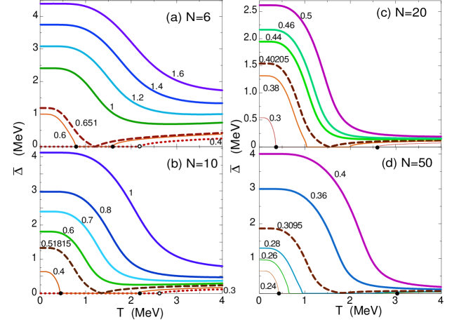
Figure 1: (Color on line) Level-weighted pairing gaps $\overline{\Delta}$ obtained within the FTBCS1 as functions of temperature $T$ at various values of pairing parameter $G$ (in MeV) indicated by the figures near the lines for several values of particle number $N$. Open circles on the axes of abscissas in panels (a) and (b) mark the values $T_{1}$ of temperature, where the FTBCS1 gap turns finite at low $G$. Full circles denote temperature $\widetilde{T}_{\rm c}$, where the gap vanishes, and $T_{2}$, where it reappears.

It is well known that, below a critical value $G_{\rm c}$ of the pairing interaction parameter, the conventional BCS theory has only a trivial solution ($\Delta=$ 0). At $G>G_{\rm c}$, the FTBCS gap decreases with increasing $T$ up to a critical value of $T=T_{\rm c}$, where it collapses, and the system undergoes a sharp SN-phase transition. The behavior of the pairing gap within the FTBCS1 theory can be inferred from Eq. (31). As a matter of fact, the increase of the QNF $\delta{\cal N}^{2}_{j}$ with $T$ leads to an increase of $\widetilde{G}_{j}$, whose consequences are qualitatively different depending on the magnitude of $G$ and particle number $N$. These features can be seen in Fig. 1, where the level-weighted pairing gaps $\overline{\Delta}$ obtained within the FTBCS1 theory at various values of the pairing interaction parameter $G$ for several particle numbers are displayed as functions of temperature $T$. They can be classified in three regions below.

In the region of strong coupling, $G\gg G_{\rm c}$, where the BCS equations have non-trivial solutions at $T=0$, and $\delta{\cal N}^{2}_{j}$ is sufficiently large so that $\widetilde{G}_{j}\gg G$, the gap $\Delta_{j}$ in Eq. (31) never collapses since whenever $T$ reaches the value $T_{\rm c}$ where the BCS gap obtained with parameter $G$ collapses, the gap $\Delta_{j}$ is always positive given $\widetilde{G}_{j}\gg G$ with a renormalized critical temperature $\widetilde{T}_{\rm c}\gg T_{\rm c}$. In this way, the sharp SN-phase transition never occurs as $\Delta_{j}$ remains always finite at $T_{\rm c}\leq T\ll\widetilde{T}_{\rm c}$ with $\widetilde{T}_{\rm c}$ continuously becoming larger with $T$. If $G$ is sufficiently large the QNF may become so large at high $T$ that the level-dependent part $\delta\Delta_{j}$ in Eqs. (29) and (30) starts to dominate and the total gap $\Delta_{j}$ will even increase with $T$. This effect is stronger when the particle number is smaller. As seen in Fig. 1, in contrast to the FTBCS gap, which collapses at $T_{\rm c}$, the FTBCS1 gaps shown as the thick solid lines are always finite. For $N\geq$ 6, the gaps decrease monotonously as $T$ increases up to $T=$ 4 MeV. This feature qualitatively agrees with the findings within alternative approaches to thermal fluctuations mentioned in the Introduction.

In the region of weak coupling, $G\leq G_{\rm c}$, where the pairing gap is zero at $T=$ 0, the increase of $\widetilde{G}_{j}$ with $T$ makes it becomes significantly greater than $G_{\rm c}$ at a certain $T=T_{\rm 1}$, allowing a non-trivial solution of the gap equation. This feature is demonstrated by the dotted lines in Figs. 1 (a) and 1 (b), where $T_{1}$ ($>$ 2 MeV) is marked by an open circle. Since the difference between the FTBCS1 gap $\Delta_{j}$ and the conventional FTBCS one, $\Delta$, is the gap $\delta\Delta_{j}$ in Eqs. (29) and (30), which arises because of the QNF $\delta{\cal N}^{2}_{j}$, it is obvious that the finite gap at $T\geq T_{1}$ is assisted by the QNF.

In the transitional region, where $G$ is slightly larger than $G_{\rm c}$, it may happens that, although $\delta{\cal N}_{j}^{2}$ increases with $T$, it is still too small so that $\widetilde{G}_{j}$ is only slightly larger than $G$, and so is $\widetilde{T}_{\rm c}$ compared to $T_{\rm c}$. As a result, the gap collapses at $T=\widetilde{T}_{\rm c}$ which is slightly larger than $T_{\rm c}$. As $T$ increases further, the mechanism of the weak-coupling region is in effect, which leads to the reappearance of the gap at $T=T_{2}>\widetilde{T}_{\rm c}$. In Fig. 1, these values $\widetilde{T}_{\rm c}$ and $T_{2}$ are denoted by full circles on the axes of absiccas for the cases with $N=$ 6, 10, 20, 50 with $G=$ 0.6, 0.4, 0.3, and 0.24 MeV, respectively. With increasing $G$, it is seen that $\widetilde{T}_{\rm c}$ increases whereas $T_{2}$ decreases so that at a certain $G$ these two temperatures coalesce. The value $G_{\rm M}$ where $\widetilde{T}_{\rm c}=T_{2}=T_{\rm M}$ is found to be 0.651, 0.51815, 0.40205 and 0.3095 MeV for $N=$ 6, 10, 20 and 50, respectively, i.e. decreases with increasing $N$. The gap obtained with $G=G_{\rm M}$ is seen decreasing with increasing $T$ from 0 to $T_{\rm M}$, where it becomes zero. Starting from $T_{\rm M}$ the gap increases again with $T$. The value $T_{\rm M}$ is found increasing with $T$ from $T_{\rm M}\simeq$ 1.2 MeV for $N=$ 6 to $T_{\rm M}\simeq$ 1.7 MeV for $N=$ 50. At $G>G_{\rm M}$ the gap remains finite at any value of $T$. For small $N$, the strong QNF even leads to an increase of the gap with $T$ at high $T$ as seen in the cases with $N=$ 6, and $G_{\rm M}<G\leq$ 1.2 MeV. With increasing $N$ the high-$T$ tail of the gap gets depleted, showing how the QNF weakens at large $N$.

The curious behavior of the level-weighted gap at weak coupling, where it appears at a certain $T=T_{1}$, and in the transitional region, where it collapses at $\widetilde{T}_{\rm c}$ and reappears at $T_{2}$, may have been caused by the well-known inadequacy of the BCS approximation (and BCS-based approaches) for weak pairing Ring . Even at $T=$ 0, Ref. Volya has shown that, whereas the exact solution predicts a condensation energy of almost 2 MeV in the doubly-closed shell ⁴⁸Ca, the BCS gives a normal Fermi-gas solution with zero pairing energy. It is expected that a proper PNP such as the number-projected HFB approach in Ref. Sheikh , if it can be practically extended to $T\neq$ 0, will eventually smooth out the transition points $T_{1}$ as well as $\tilde{T}_{\rm c}$ and $T_{2}$ in Fig. 1.

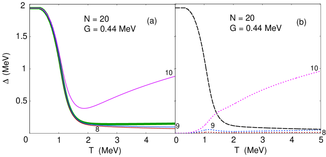
Figure 2: (Color on line) Level-dependent pairing gap $\Delta_{j}$ (29) and level-weighted pairing gap $\overline{\Delta}$ (70) obtained within the FTBCS1 as functions of temperature $T$ for $N=$ 20 and $G=$ 0.44 MeV. Thick solid lines represent the level-weighted gaps $\overline{\Delta}$. Thin solid lines denote the level-dependent gaps $\Delta_{j}$ corresponding to the $j$-th orbitals, whose level numbers $j$ are marked at the lines. Dashed and dotted lines stand for the level-independent part (quantal component), $\Delta$, and the level-dependent one (thermal component), $\delta\Delta_{j}$, of the FTBCS1 gap $\Delta_{j}$ (29), respectively.

To have an insight into the source that causes the high-$T$ tail of the FTBCS1 gap we plot in Fig. 2 the examples for the level-weighted gaps $\overline{\Delta}$ (70) along with the level-dependent gaps $\Delta_{j}$ (29), which are obtained for $N=$ 20 and $G=$ 0.44 MeV. It is seen from this figure that the level-independent part (quantal component) $\Delta$ of the gap [dashed lines in Fig. 2 (b)] also has a high-$T$ tail although it is much depleted compared to the total gap $\Delta_{j}$, which includes the level-dependent part $\delta\Delta_{j}$. This figure also reveals that the QNF has the strongest effect on the levels closest to the Fermi surface, which are the 10th and 11th levels. In this figure, the results for the 11th level are not showed as they coincide with those for the 10th one due to the particle-hole symmetry, which is well preserved within the FTBCS1. For the rest of levels, the effect of QNF is much weaker. With increasing the particle number $N$, the number of levels away from the Fermi surface becomes larger, whose contribution in the gap $\overline{\Delta}$ outweighs that of the levels closest to the Fermi surface. This explains why the high-$T$ tail of the level-weighted gap $\overline{\Delta}$ is depleted at large $N$. When $N$ becomes very large, this tail practically vanishes as the total effect of QNF becomes negligible. In this limit, the temperature dependence of the pairing gap approaches that predicted by the standard BCS theory, which is well valid for infinite systems.

III.2.2 Corrections due to particle-number projection and SCQRPA

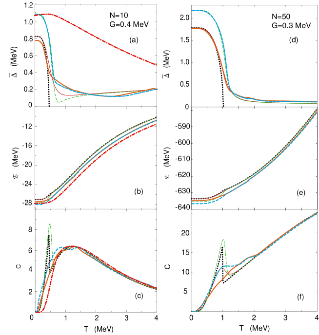
Figure 3: (Color on line) Level-weighted pairing gaps (a, d), total energies (b, e), and heat capacities (c, f) as functions of temperature $T$, obtained for $N=$ 10 [(a) – (c)], and $N=$ 50 [(d) – (f)]. The dotted, thin solid, thick solid lines show the FTBCS, FTBCS1, and FTBCS1+SCQRPA results, respectively. The predictions by the FTLN1 and FTLN1+SCQRPA are presented by the thin and thick dashed lines, respectively. The dash-dotted lines in (a) – (c) denote the exact results. The calculations of the mass operator and quasiparticle damping within the SCQRPA were performed using $\varepsilon=$ 0.05 MeV.

Show in Fig. 3 are the level-weighted pairing gaps $\overline{\Delta}$, total energies ${\cal E}$, and heat capacities $C$, obtained within the FTBCS, FTBCS1, FTLN1, FTBCS1+SCQRPA, and FTLN1+SCQRPA for the systems with $N=$ 10 ($G=$ 0.4 MeV) and $N=$ 50 ($G=$ 0.3 MeV). As we want to see the effect of QNF for the case with small $\Delta(T=0)$ without any phase transition points at $\widetilde{T}_{\rm c}$ and $T_{2}$, we choose to neglect, for this particular test, the self-energy term $-Gv_{j}^{2}$ in the single-particle energy. For $N=$ 10 e.g., this increases the gap at $T=$ 0 by around 14$\%$, to around 0.8 MeV, but the change in the total energy is found to be negligible. Different from the common practice, which usually neglects the terms $\sim-G\sum_{j}\Omega_{j}v_{j}^{4}$ in calculating the total energy ${\cal E}$, the latter is calculated in the present article by averaging the complete pairing Hamiltonian (3). For $N=$ 10 and $G=$ 0.4 MeV e.g., this causes a shift of total energy down by around 2 MeV ($\sim 8\%$) and 1 MeV ($\sim 10.4\%$) at $T=$ 0 and 4 MeV, respectively.

As has been discussed in Sec. II.3.2, Fig. 3 demonstrates that, although the LN method significantly improves the agreement between the predictions by the FTBCS1 theory with the exact results for the pairing gap and total energy at low $T$, it fails to do so at $T\geq T_{\rm c}$, where all approximated results for the pairing gap coalesce and clearly differ from the exact result (for $N=$ 10). The reason is partly due to the fact that, strictly speaking, there is no pairing gap in the exact solution MBCS3 . The dash-dotted line, representing the exact result in Fig. 3 (a) is the effective gap (canonical gap) extracted from the pairing energy. The latter is the difference between the exact total energy and the that of the single-particle mean field (Hartre-Fock) energies. The canonical gap includes correlations caused by the fluctuations of the order parameter, only a part of which is taken into account within the FTBCS1 in terms of QNF. It reduces to the BCS pairing gap only within the mean field approximation and the grand canonical ensemble

The corrections caused by the SCQRPA are found to be significant for small $N$ ($N=$ 10), in particular for the pairing gap in the region $T_{\rm c}<T<$ 1.5 MeV [Fig. 3 (a)]. At $T<T_{\rm c}$, the predictions by the FTLN1+SCQRPA are closer to the exact results than those by the FTBCS1+SCQRPA. At $T>T_{\rm c}$ both approximations offer nearly the same results. They produce the total energies and heat capacities, which are much closer to the exact values as compared to the FTBCS1 and FTLN1 results, as shown in Figs. 3 (b) and 3 (c). What remarkable here is that the SCQRPA correction indeed smears out all the trace of the SN phase transition in the pairing gap as well as energy and heat capacity.

For large $N$ ($N=$ 50), the effect of SCQRPA corrections is much smaller, although still visible. It depletes the spike, which is the signature of the SN phase transition around $T_{\rm c}$ in the heat capacity, leaving only a broad bump between 0 $<T<$ 2 MeV [Fig. 3 (f)]. The exact results are not available because, for large particle numbers, one faces technical problems of diagonalizing matrices of huge dimension, all the eigenvalues of which should be included in the partition function to describe correctly the total energy and heat capacity.

III.3 Results by using realistic single-particle spectra

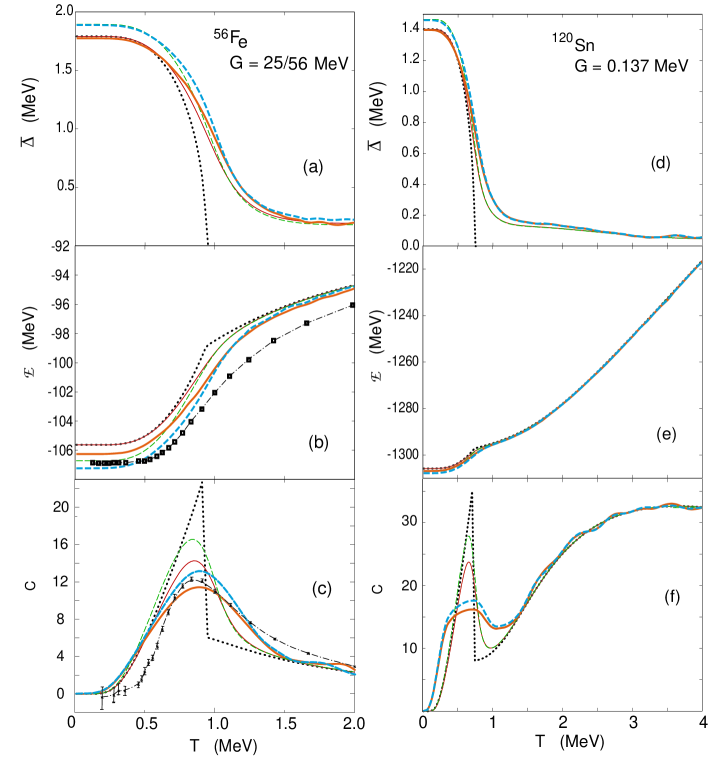
Figure 4: (Color on line) Level-weighted pairing gaps, total energies, and heat capacities for 10 neutrons in the $1f_{7/2}2p_{3/2}2p_{1/2}1f_{5/2}$ shell of ⁵⁶Fe and all neutron bound states of ¹²⁰Sn as functions of $T$ ($\varepsilon=$ 0.1 MeV). Notations are as in Fig. 3. In (b) and (c), the predictions by the finite-temperature quantum Monte Carlo method QMC are shown as boxes and crosses with error bars connected by dash-dotted lines.

The level-weighted gaps, total energies, and heat capacities, obtained for neutrons in ⁵⁶Fe and ¹²⁰Sn within the same approximations are displayed as functions of $T$ in Fig. 4. The results of calculations for 10 neutrons in the $1f_{7/2}2p_{3/2}2p_{1/2}1f_{5/2}$ shell using $G=$ 25/26 MeV are plotted in Figs. 4 (a) – 4 (c) as functions of $T$ within the same temperature interval as that in Ref. QMC . They clearly show that the SCQRPA corrections bring the FTBCS1 (FTLN1)+SCQRPA results closer to the predictions by the FTQMC method for the total energy and heat capacity (No results for the pairing gap are available within the FTQMC method in Ref. QMC ). In heavy nuclei, such as ¹²⁰Sn, the effects caused by the SCQRPA corrections are rather small on the pairing gap and total energy. In both nuclei, the pairing gaps do not collapse at $T=T_{\rm c}$, but monotonously decrease with increasing $T$, and the signature of the sharp SN-phase transition seen as a spike at $T=T_{\rm c}$ in the heat capacities is strongly smoothed out within the FTBCS1+SCQRPA.

III.4 Self-consistent and statistical treatments of quasiparticle occupation numbers

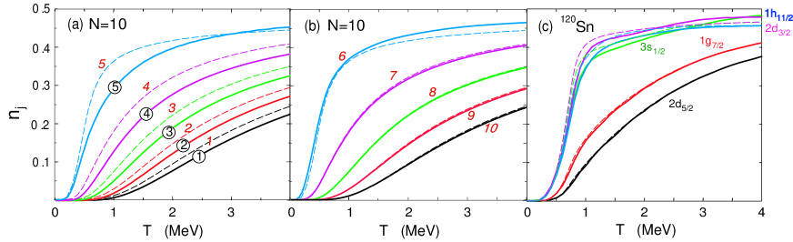
Figure 5: (Color on line) Quasiparticle occupation numbers for $N=$ 10 with $G=$ 0.4 MeV (a, b) and ¹²⁰Sn with $G=$ 0.137 MeV (c) as functions of $T$. In (a) and (b) the solid lines are predictions within FTBCS1+SCQRPA for the levels numerated by the numbers in the circles starting from the lowest ones. The dashed lines, numerated by the italic numbers, show the corresponding results obtained within the FTBCS1. In (c) predictions for the neutron orbitals of the (50 - 82) shell in ¹²⁰Sn, obtained within the FTBCS1 and FTBCS1+SCQRPA, are shown as the dashed and solid lines, respectively.

The quasiparticle occupation numbers $n_{j}$ as predicted by the FTBCS1 and FTBCS1+SCQRPA for all quasiparticle levels in the system with $N=$ 10, $G=$ 0.4 MeV, and for the orbitals within the (50 - 82) shell in ¹²⁰Sn ($G=$ 0.137 MeV) are shown in Fig. 5 as functions of $T$. While the $ph$ symmetry is preserved within the FTBCS1 ($n_{j}=n_{j}^{\rm FD}$) in the sense that the values for $n_{j}^{\rm FD}$ are identical for the single-particle levels located symmetrically from the Fermi level [Compare the dashed lines in Figs. 5 (a) and 5 (b)], it is no longer the case after taking into account dynamic coupling to SCQRPA vibrations. This is particularly clear in light systems [See the solid lines in Figs. 5 (a) and 5 (b)]. This deviation of $n_{j}$ from the Fermi-Dirac distribution of free quasiparticles, however, turns out to be quite small in realistic heavy nuclei, such as ¹²⁰Sn, as shown in Fig. 5 (c).

III.5 Comparison between FTBCS1 and MBCS

In Refs.  MBCS1 ; MBCS2 ; MBCS3 ; MBCS4 the MBCS theory has been developed, which also produces a nonvanishing pairing gap at high $T$. Therefore, it is worthwhile to draw a comparison between the MBCS theory and the present one. Both approaches include the same QNF (27) as the microscopic source, which smoothes out the sharp SN-phase transition and leads to the high-$T$ tail of the pairing gap. This high-$T$ tail has been shown to be sensitive to the size of the configuration space in either approach. However, due to different assumptions in these two approaches, the functional dependences of $\delta\Delta_{j}$ on the QNF $\delta{\cal N}_{j}^{2}$ are different. As a result, the FTBCS1 gap is level-dependent, whereas the MBCS one is not. The most important advantage of the FTBCS1 over the MBCS theory is that the solution of the FTBCS1 gap equation (29) is never negative. Moreover, at moderate and strong couplings, where the FTBCS1 gap is finite, its behavior as a function of temperature bears no singularities in any configuration spaces for any value of $N\geq$ 2. The MBCS gap, on the other hand, is free from singularities only up to a certain temperature $T_{\rm M}$, which is around 1.75 – 2.3 MeV within the Richardson model with $\Omega=N=$ 10 and increases almost linearly with $N$ to reach $T_{\rm M}\simeq$ 24 MeV for $\Omega=N=$ 100 MBCS3 (For detail discussions see Refs. MBCS3 ; MBCS4 and references therein). However, the mean-field contraction used to factorize the QNF within the FTBCS1 to the form (27) may have left out some higher-order fluctuations, which can enhance the total effect of the QNF. It might also be the reason that causes the phase transition temperatures $T_{1}$, $\widetilde{T}_{\rm c}$ and $T_{2}$ at weak coupling and in the transitional region, discussed in Sec. III.2.1. Meanwhile, the MBCS theory is based on the strict requirement of restoring the unitarity relation for the generalized single-particle density matrix MHFB , which brings in the QNF $\delta{\cal N}_{j}^{2}$ (27) without the need of using a mean-field contraction. As a result, the effect of QNF within the MBCS theory is stronger than that predicted within the FTBCS1 and/or FTBCS1+SCQRPA, which can be clearly seen by comparing, e.g., Fig. 4 (d) above and Fig. 4 of Ref. MHFB . Whether this means that the secondary Bogoliubov’s transformation properly includes or exaggerates the effect of coupling to configurations beyond the quasiparticle mean field within the MBCS theory remains to be investigated. Another question is also open on whether the MBCS theory can be improved by coupling the modified quasiparticles to the modified QRPA vibrations. The answer to these issues may be a subject for future study.

IV CONCLUSIONS

The present work extends the BCS1+SCQRPA theory, derived in Ref. SCQRPA for a multilevel pairing model, to finite temperature. The resulting FTBCS1+SCQRPA theory includes the effect of QNF as well as dynamic coupling of quasiparticles to pairing vibrations. This theory also incorporates the corrections caused by the particle-number projection within the LN method.

We have carried out a thorough test of the developed approach within the Richardson model as well as two realistic nuclei, ⁵⁶Fe and ¹²⁰Sn. The analysis of the obtained pairing gaps, total energies, and heat capacities leads to the following conclusions:

1) The FTBCS1 (with or without SCQRPA corrections) microscopically confirms that, in the region of moderate and strong couplings, the quasiparticle-number fluctuation smoothes out the sharp SN phase transition, predicted by the FTBCS theory. As a result, the gap does not collapse at $T=T_{\rm c}$, but has a tail, which extends to high temperature $T$.

2) The correction due to the particle-number projection within the LN method to the pairing gap is significant at $T\ll T_{\rm c}$, which leads to a steeper temperature dependence of the pairing gap in the region around $T_{\rm c}$. At the same time, the SCQRPA correction smears out the signature of a sharp SN phase transition even in heavy realistic nuclei such as ¹²⁰Sn.

3) The dynamic coupling to SCQRPA vibrations causes the deviation of the quasiparticle occupation number from the Fermi-Dirac distribution for non-interacting fermions. However, for a realistic heavy nucleus such as ¹²⁰Sn, this deviation is negligible. Consequently, in these nuclei, the FTBCS1 and FTBCS1+SCQRPA predict similar results for the pairing gap and total energy. At the same time, for light systems, this deviation is stronger, therefore, the FTBCS1+SCQRPA offers a better approximation than the FTBCS1 in the study of thermal pairing properties of these nuclei.

The fact that the total energies and heat capacities obtained within the FTBCS1+SCQRPA predictions agree reasonably well with the exact results for $N=$ 10 as well as those obtained within the finite-temperature quantum Monte Carlo method for ⁵⁶Fe shows that the FTBCS1+SCQRPA can be applied in further study of thermal properties of finite systems such as nuclei, where pairing plays an important role. Compared to existing methods, the merit of the present approach lies in its fully microscopic derivation and simplicity when it is applied to heavy nuclei with strong pairing, where the effect of coupling to SCQRPA is negligible so that the solution of the SCQRPA can be avoided. In this case, thermal pairing can be determined solely by solving the FTBCS1 gap equation, which is technically as simple as the FTBCS one, whereas the exact diagonalization is impracticable (at $T\neq$ 0).

As the next step in improving the developed approach, we will include the effect of angular momentum in this approach. This study is now underway and the results will be reported in a forthcoming article Hung .

Appendix A Factorization of $\langle{\cal A}_{j}^{\dagger}{\cal A}_{j^{\prime}}\rangle$

The factorization of the screening factor $\langle{\cal A}^{\dagger}_{j}{\cal A}_{j^{\prime}}\rangle$ is not unique as it can be carried out in at least two ways, which lead to different results. In the first way, one can perform the mean-field contraction by using the Wick’s theorem (WT) to obtain

$$\langle{\cal A}^{\dagger}_{j}{\cal A}_{j^{\prime}}\rangle^{\rm WT}\simeq\delta_{jj^{\prime}}n_{j}^{2}~{}.$$ (73)

In the second way, one uses the Holstein-Primakoff’s (HP) boson representation HP

$${\cal A}_{j}^{\dagger}=b_{j}^{\dagger}\sqrt{1-\frac{b_{j}^{\dagger}b_{j}}{\Omega_{j}}}~{},\hskip 14.22636pt{\cal A}_{j}=\sqrt{1-\frac{b_{j}^{\dagger}b_{j}}{\Omega_{j}}}b_{j}~{},\hskip 14.22636pt{\cal N}_{j}=2b_{j}^{\dagger}b_{j}~{},$$ (74)

with boson operators $b_{j}^{\dagger}$ and $b_{j}$ to obtain

$$\langle{\cal A}^{\dagger}_{j}{\cal A}_{j^{\prime}}\rangle^{\rm HP}\simeq\delta_{jj^{\prime}}\Omega_{j}n_{j}(1-2n_{j})~{}.$$ (75)

The lowest order of the HP boson representation implies that operators ${\cal A}_{j}^{\dagger}$ and ${\cal A}_{j}$ are ideal bosons $b_{j}^{\dagger}$ and $b_{j}$, respectively, i.e. setting ${\cal D}_{j}=$ 1 in Eq. (6). It is in fact the well-known quasiboson approximation (QBA), which is widely used in the derivation of the QRPA equations. The QBA leads to

$$\langle{\cal A}^{\dagger}_{j}{\cal A}_{j^{\prime}}\rangle^{\rm QBA}\simeq\frac{1}{2}\delta_{jj^{\prime}}\langle{\cal N}_{j}\rangle=\delta_{jj^{\prime}}\Omega_{j}n_{j}~{}.$$ (76)

As for the screening factor $\langle{\cal A}^{\dagger}_{j}{\cal A}_{j^{\prime}}^{\dagger}\rangle$, it vanishes in these approximations.

Using these results, we obtain the same form of Eq. (29) for the pairing gap, except that now $\epsilon_{j}^{\prime}=\epsilon_{j}$, and the level-dependent part $\delta\Delta_{j}$ from Eq. (30) becomes

$$\delta\Delta_{j}^{\rm WT}\simeq 2Gu_{j}v_{j}n_{j}~{},$$ (77)

$$\delta\Delta_{j}^{\rm HP}\simeq 2Gu_{j}v_{j}\frac{n_{j}[1-\Omega_{j}+(2\Omega_{j}-1)n_{j}]}{1-2n_{j}}~{},$$ (78)

$$\delta\Delta_{j}^{\rm QBA}\simeq 2Gu_{j}v_{j}\frac{n_{j}(1-\Omega_{j}-n_{j})}{1-2n_{j}}~{},$$ (79)

which correspond to the approximations using the Wick’s theorem, HP representation, and the QBA, respectively.

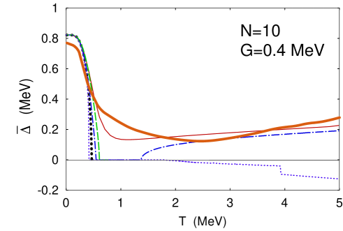
Figure 6: (Color on line) Level-weighted gaps for $N=$ 10 with $G=$ 0.4 MeV as predicted by the WT (dashed), HP (dash-dotted), and QBA (thin dotted) approximations in comparison with the FTBCS (thick dotted), FTBCS1 (thin solid), and FTBCS1+SCQRPA (thick solid) results.

The level-weighted gaps $\overline{\Delta}$ obtained for $N=$ 10 and $G=$ 0.4 MeV within these approximations are compared with the FTBCS, FTBCS1 and FTBCS1+SCQRPA results in Fig. 6. At $T<$ 1 MeV, all three approximations, WT, HP, and QBA, predict the gaps close to the FTBCS one, but collapse at different $T_{\rm c}$, namely $T_{\rm c}^{\rm QBA}<T_{\rm c}^{\rm FTBCS}<T_{\rm c}^{\rm HP}<T_{\rm c}^{\rm WT}$. At $T\simeq$ 1.2 MeV the HP gap reappears and increases with $T$ to reach the values comparable with those predicted by the FTBCS1 and FTBCS1+SCQRPA at $T>$ 2 MeV. From this comparison, one can see that the mean-field contraction (73) for $\langle{\cal A}_{j}^{\dagger}{\cal A}_{j^{\prime}}\rangle$ includes only a tiny fraction of the QNF because it produces a finite gap at $T>T_{\rm c}^{\rm FTBCS}\simeq$ 0.5 MeV, but this gap collapses again at $T_{\rm c}^{\rm WT}\simeq$ 0.6 MeV. The HP boson representation, on the other hand, is able to take into account the effect of QNF at hight $T$ leading to a finite gap at $T>$ 1.38 MeV, but fails to account for this effect at intermediate temperatures 0.55 $\leq T\leq$ 1.38 MeV. The QBA produces essentially the same result as that of the conventional FTBCS at low $T$ with a slightly lower critical temperature $T_{\rm c}^{\rm QBA}\simeq$ 0.43 MeV. However, it causes a negative $\overline{\Delta}$ at $T>$ 1.9 MeV.

References

- (1) J. Bardeen, L. Cooper, and J. Schrieffer, Phys. Rev. 108, 1175 (1957)
- (2) V. J. Emery, and A. M. Sessler, Phys. Rev. 119 248 (1960)
- (3) L.D. Landau and E.M. Lifshitz, Course of Theoretical Physics, Vol. 5: Statistical Physics (Moscow, Nauka, 1964) pp. 297, 308.
- (4) L.G. Moretto, Phys. Lett. B 40, 1 (1972).
- (5) A.L. Goodman, Nucl. Phys. A 352, 30 (1981).
- (6) A.L. Goodman, Phys. Rev. C 29, 1887 (1984).
- (7) R. Rossignoli, P. Ring, and N.D. Dang, Phys. Lett. B 297, 9 (1992); N.D. Dang, P. Ring, and R. Rossignoli, Phys. Rev. C 47, 606 (1993).
- (8) V. Zelevinsky, B.A. Brown, N. Frazier, and M. Horoi, Phys. Rep. 276, 85 (1996).
- (9) D.J. Dean et al., Phys. Rev. Lett. 74, 2909 (1995).
- (10) S. Frauendorf, N.K. Kuzmenko, V.M. Mikhajlov, and J.A. Sheikh, Phys. Rev. B 68, 024518 (2003); J.A. Sheikh, R. Palit, and S. Frauendorf, Phys. Rev. C 72, 041301(R) (2005).
- (11) N.D. Dang and A. Arima, Phys. Rev. C 68, 014318 (2003).
- (12) N. Dinh Dang and V. Zelevinsky, Phys. Rev. C 64, 064319 (2001).
- (13) N. Dinh Dang and A. Arima, Phys. Rev. C 67, 014304 (2003).
- (14) N. Dinh Dang, Nucl. Phys. A 784, 147 (2007).
- (15) N.D. Dang, Phys. Rev. C 76, 064320 (2007).
- (16) K. Kaneko and M. Hasegawa, Phys. Rev. C 72, 024307 (2005).
- (17) N.D. Dang and K. Tanabe, Phys. Rev. C 74, 034326 (2006).
- (18) N.Q. Hung and N.D. Dang, Phys. Rev. C 76, 054302 (2007), Ibid. 77, 029905(E) (2008).
- (19) R.W. Richardson, Phys. Lett. 3, 277 (1963), Phys. Lett. 5, 82 (1963), Phys. Lett. 14, 325 (1965).
- (20) J. Dukelsky and P. Schuck, Phys. Lett. B 464, 164 (1999).
- (21) J. Dukelsky and P. Schuck, Nucl. Phys. A 512, 466 (1990); A. Rabhi, R. Bennaceur, G. Chanfray, and P. Schuck, Phys. Rev. C 66, 064315 (2002).
- (22) M. Sambataro and N. Dinh Dang, Phys. Rev. C 59, 1422 (1999).
- (23) H.C. Pradhan, Y. Nogami, and J. Law, Nucl. Phys. A 201, 357 (1973).
- (24) M. Anguiano, J.L. Egido, and L.M. Robledo, Phys. Lett. B 545, 62 (2002).
- (25) H.M. Sommermann, Ann. Phys. (NY) 151, 163 (1983).
- (26) N. D. Dang, J. Phys. G 11, L125 (1985).
- (27) N.N. Bogolyubov and S.V. Tyablikov, Soviet Phys.-Doklady 4, 60 (1959) [Dokl. Akad. Nauk SSSR 126, 53 (1959)].
- (28) D.N. Zubarev, Soviet Physics Uspekhi 3, 320 (1960) [Usp. Fiz. Nauk 71, 71 (1960)].
- (29) A. Volya, B. A. Brown, V. Zelevinsky, Phys. Lett. B 509, 37 (2001).
- (30) S. Rombouts, K. Heyde, and N. Jachowicz, Phys. Rev. C 58, 3295 (1998).
- (31) N. Dinh Dang, Z. Phys. A 335, 253 (1990).
- (32) P. Ring and P. Schuck, The Nuclear Many-Body Problem (Springer-Verlag, NY, 1980).
- (33) J.A. Sheikh, P. Ring, E. Lopes, and R. Rossignoli, Phys. Rev. C 66, 044318 (2002).
- (34) N. Quang Hung and N. Dinh Dang, in preparation.
- (35) T. Holstein and H. Primakoff, Phys. Rev. 58, 1098 (1940).