Stability of Fock states in a two-component Bose-Einstein condensate with a regular classical counterpart

Abstract

We study the stability of a two-component Bose-Einstein condensate (BEC) in the parameter regime in which its classical counterpart has regular motion. The stability is characterized by the fidelity for both the same and different initial states. We study as initial states the Fock states with definite numbers of atoms in each component of the BEC. It is found that for some initial times the two Fock states with all the atoms in the same component of the BEC are stabler than Fock states with atoms distributed in the two components. An experimental scheme is discussed, in which the fidelity can be measured in a direct way.

I Introduction

In many research fields, such as Bose-Einstein condensation (BEC) and quantum information processing, stable and coherent manipulation of quantum states is of crucial importance lukin . In fact, the instability issue of BEC in dilute gases bec has been constantly addressed for its crucial role in the control, manipulation, and even future application of this newly formed matter, including dynamical instability dyinst , Landau or superfluid instability Landinst , modulation instability modins ; BKPV07 , and quantum fluctuation instability smerzianglin . It is found that instability may break the coherence among the atoms and lead to collapse of BEC liukick .

Recently, the stability of the quantum motion of BEC systems under small perturbation, which is measured by the so-called quantum Loschmidt echo or fidelity, has been studied pra05-bec ; MH08 . Here, the fidelity is defined as the overlap of two states obtained by evolving the same initial state under two slightly different Hamiltonians Peres84 ; nc-book ; gc-book . Explicitly, it is $M(t)=|m(t)|^{2}$, where $m(t)$ is the fidelity amplitude for an initial state $|\Phi_{0}\rangle$, defined as

$$m(t)=\langle\Phi_{0}|{\rm exp}(iHt/\hbar){\rm exp}(-iH_{0}t/\hbar)|\Phi_{0}\rangle.$$ (1)

Here $H_{0}$ and $H=H_{0}+\epsilon V$ are the unperturbed and perturbed Hamiltonians, respectively, with $\epsilon$ a small quantity and $V$ a generic perturbing potential.

Fidelity decay has been well studied in quantum systems whose classical counterparts have chaotic motion JP01 ; JSB01 ; BC02 ; CT02 ; PZ02 ; fid-wg ; VH03 ; STB03 ; Vanicek04 ; GPSZ06 . Related to the perturbation strength, previous investigations show the existence of at least three regimes of fidelity decay. (i) In the perturbative regime with sufficiently weak perturbation, in which the typical transition matrix element is smaller than the mean level spacing, the fidelity has a Gaussian decay Peres84 ; JSB01 ; CT02 . (ii) Above the perturbative regime, the fidelity has an exponential decay with a rate proportional to $\epsilon^{2}$, usually called the Fermi-golden-rule (FGR) decay of fidelity JP01 ; JSB01 ; BC02 ; CT02 ; PZ02 ; fid-wg . (iii) Above the FGR regime is the Lyapunov regime in which $M(t)$ usually has an approximate exponential decay with a perturbation-independent rate; the decay rate of the fidelity is given by the Lyapunov exponent of the underlying classical dynamics, when the classical counterpart of the quantum system has a homogeneous phase space JP01 ; JSB01 ; BC02 ; fid-wg ; VH03 ; STB03 .

For quantum systems whose classical counterparts have regular motion, many investigations in the decaying behavior of fidelity have also been carried out (see, e.g., Ref. PZ02 ; JAB03 ; PZ03 ; SL03 ; Vanicek04 ; WH05 ; Comb05 ; HBSSR05 ; pra05-bec ; GPSZ06 ; WB06 ; pre07 ), however, the situation is still not as clear as in the case of quantum chaotic systems. The point is that fidelity decay in quantum regular systems exhibits notable initial-state dependence. (In quantum chaotic systems, the main feature of fidelity decay is initial-state independent beyond a short initial time.) The most thoroughly studied initial states are narrow Gaussian wave packets (coherent states), for which the semiclassical theory and numerical simulations show that the fidelity has, roughly speaking, a Gaussian decay followed by a long-time power law decay PZ02 ; WH05 ; pre07 . Some other types of initial states of practical interest have also been studied numerically, e.g., the fidelity of an initial maximally entangled (N-GHZ) state is shown to have an interesting oscillating behavior pra05-bec .

The above considerations motivate our interest in the stability of a two-component BEC cornell , which is exposed to a pulsed laser field coupling two internal states of the atoms in the BEC. This BEC system possesses a classical counterpart, which has chaotic or regular motion depending on both the strength of the coupling field and that of the interaction among the atoms pra05-bec . In Ref. pra05-bec , the fidelity of initial coherent states in this BEC system has been studied and found in agreement with previous analytical predictions in both cases with chaotic and regular motion in the classical limit. We remark that, more recently, the fidelity approach has also been employed in the study of the stability of another BEC system, which starts from the ground state MH08 .

In this paper, we study the stability of the quantum motion of the same BEC system as in Ref. pra05-bec . However, here we are interested in the stability of initial Fock states, which have definite numbers of atoms occupying each of the two components of the BEC, and in the parameter regime in which the classical counterpart of the BEC system has regular motion. In particular, we are interested in whether some Fock states are more stable than others. Knowledge about the stability properties of this type of initial states may be useful for potential application of BEC in fields such as quantum information youli . As in Ref. pra05-bec , we still consider the stability issue caused by small perturbation due to imperfect control of the coupling field and use fidelity to characterize the stability, with the difference between $H$ and $H_{0}$ in Eq. (1) given by a small change in the strength of the coupling field.

Presently, there is no analytical prediction for fidelity decay of initial Fock states, therefore, our investigation is mainly based on numerical simulations. Interestingly, our numerical results show that, for some initial times, initial Fock states with all the atoms in the same component of the BEC are more stable than other Fock states. To see whether or not this property is due to the specific measure given in Eq. (1), we have also studied the behavior of a more general form of the fidelity, which is the overlap of the time evolution of two different initial Fock states under two slightly different Hamiltonians. Our numerical simulations for this more general fidelity give consistent results.

The paper is organized as follows: In the second section, we discuss briefly the two-component BEC model. Section III is devoted to a study of fidelity for the same initial Fock states. In Sec. IV, we introduce and study numerically the more general fidelity mentioned above for two different initial states. Conclusions are given in Sec. V. An experimental scheme for measuring fidelity of the quantum motion of a two-component BEC is discussed in the Appendix.

II Physical Model

We consider the same BEC system as in Ref. pra05-bec , specifically, cooled ⁸⁷Rb atoms with two different hyperfine states $F=1,m_{F}=-1$ and $F=2,m_{F}=+1$. The total number of the atoms in the BEC is $N$. A near resonant, pulsed radiation laser field is used to couple the two internal states. Within the standard rotating-wave approximation, the Hamiltonian describing the transition between the two internal states reads

$$\hat{H}=\frac{\mu}{2}(\hat{a}_{1}^{\dagger}\hat{a}_{1}-\hat{a}_{2}^{\dagger}\hat{a}_{2})+\frac{g}{4}(\hat{a}_{1}^{\dagger}\hat{a}_{1}-\hat{a}_{2}^{\dagger}\hat{a}_{2})^{2}$$

$$+\frac{K}{2}(\hat{a}_{1}^{\dagger}\hat{a}_{2}+\hat{a}_{2}^{\dagger}\hat{a}_{1})\sum_{n}\delta(t-nT),$$ (2)

where $K$ is the coupling strength proportional to the laser field. Here we suppose that the laser field used to couple the two states is turned on only at certain times with a period $T$. The operators $\hat{a}_{1},\,\hat{a}_{1}^{\dagger},\,\hat{a}_{2}$, and $\hat{a}_{2}^{\dagger}$ are boson annihilation and creation operators for the two components, respectively. The parameters are $K=\hbar\Omega_{R},\,g=\frac{2\pi\hbar^{2}}{m}\eta(2a_{12}-a_{11}-a_{22}),\,\mu=-\delta+(4N\pi\hbar^{2}/m)\eta(a_{11}-a_{22}).$ Here, $\Omega_{R}$ is the Rabi frequency; $a_{ij}$ is the $s$-wave scattering amplitude; $\delta$ is the detuning of lasers from resonance, very small and negligible in our case; $m$ is the mass of atom; $\eta$ is a constant of order one independent of the hyperfine index, relating to an integral of equilibrium condensate wave function leggett .

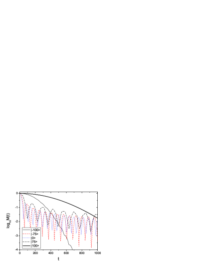
Figure 1: Decay of fidelity for $K=1$, $g_{c}=0.2$, $L=100$, and $\sigma=0.1$. The initial states are Fock states $|l\rangle$ of $l=-100$ (thin solid curve), -75 (dashed curve), 0 (dotted curve), 75 (dashed-dotted curve), and 100 (thick solid curve), respectively. The initial decay of the fidelity of the two states $|L\rangle$ and $|-L\rangle$ is much slower than that of the other three Fock states.

The above Hamiltonian can be written in terms of the SU(2) generators anglin ,

$$\hat{L}_{x}=\frac{\hat{a}_{1}^{\dagger}\hat{a}_{2}+\hat{a}_{2}^{\dagger}\hat{a}_{1}}{2},\hat{L}_{y}=\frac{\hat{a}_{1}^{\dagger}\hat{a}_{2}-\hat{a}_{2}^{\dagger}\hat{a}_{1}}{2i},\hat{L}_{z}=\frac{\hat{a}_{1}^{\dagger}\hat{a}_{1}-\hat{a}_{2}^{\dagger}\hat{a}_{2}}{2},$$ (3)

which gives

$$\hat{H}=\mu\hat{L}_{z}+g\hat{L}_{z}^{2}+K\delta_{T}(t)\hat{L}_{x}.$$ (4)

The Floquet operator describing the quantum evolution in one period is pra05-bec ; PZ02

$$\hat{U}=\exp[-i(\mu\hat{L}_{z}+g\hat{L}_{z}^{2})T]\exp(-iK\hat{L}_{x}),$$ (5)

where the Planck constant is set unit unless otherwise stated. Since the overall scaling of the Hamiltonian does not influence dynamical properties of the system, we will set $\mu$ unit.

The Hilbert space for the system is spanned by the eigenstates of $\hat{L}_{z}$, denoted by $|l\rangle$ with $l=-L,-L+1,\ldots,L$, where $L=N/2$. These states $|l\rangle$ are the Fock states. Using $N_{1}$ and $N_{2}$ to denote the numbers of the atoms in the two components, respectively, with $N=N_{1}+N_{2}$, we have $l=(N_{1}-N_{2})/2$. Hence, $|l\rangle$ is the state with $N_{1}=(L+l)$ atoms in the first component and with $N_{2}=(L-l)$ atoms in the second component. In particular, the two states with all the atoms in one of the two components are $|-L\rangle$ and $|L\rangle$. The SU(2) representation of the system discussed above is quite convenient for the study of properties of the Fock states $|l\rangle$.

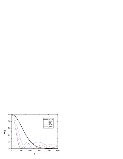
Figure 2: Decay of fidelity for $K=1,g_{c}=0.2,L=100$, and $\sigma=0.1$. The initial states are Fock states $|l\rangle$ of $l=100,99,98$ and 97, respectively.

Note that for some specific choice of the parameters the system degenerates to the quantum kicked top model kicktop . As in the kicked top model, an effective Planck constant can be introduced, $\hbar_{\rm eff}=1/L$, which will be written as $\hbar$ in what follows for brevity. The system has a classical counterpart in the limit $N\to\infty$.

III Fidelity decay for initial Fock states

As mentioned in the Introduction, we consider a small perturbation due to imperfect control of the coupling field. Specifically, for an unperturbed Hamiltonian $H_{0}$ with the form given on the right-hand side of Eq. (4), the perturbed Hamiltonian ($H_{0}+\epsilon V$) is given by the change $K\to K+\epsilon$. Denoting the one-period evolution operators corresponding to the unperturbed and the perturbed Hamiltonians by $\hat{U}$ and $\hat{U}_{\epsilon}$, respectively, the fidelity amplitude $m(t)$ is now written as

$$m(t=nT)=\langle\Phi_{0}|\left(\hat{U}_{\epsilon}^{\dagger}\right)^{n}\circ\left(\hat{U}\right)^{n}|\Phi_{0}\rangle,$$ (6)

with $|\Phi_{0}\rangle$ indicating the initial state. Fast decay of the fidelity means rapid lose of information during the quantum evolution in the presence of the perturbation. For small $\epsilon$, it is usually convenient to use $\sigma=\epsilon/\hbar$ as a measure for the strength of quantum perturbation.

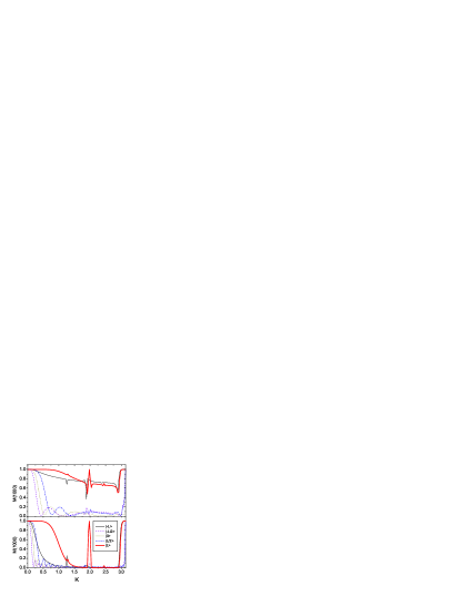
Figure 3: Values of $M(t)$ for $t=1000$, as a function of $K$. The five curves correspond to five initial Fock states: the thin solid curve for $|-L\rangle$, dashed curve for $|-L/2\rangle$, dotted curve for $|0\rangle$, dashed-dotted curve for $|L/2\rangle$, and thick sold curve for $|L\rangle$. Parameters are $L=100,g_{c}=0.2$, and $\sigma=0.01$ for the upper panel and $\sigma=0.04$ for the lower panel.

In this paper, we consider only the parameter regime in which the corresponding classical system has regular motion (see Ref. pra05-bec for details of the regime). We have carried out numerical investigations in the fidelity decay of initial Fock states $|l\rangle$ in this parameter regime. It is found that the two Fock states with $|l|=L$, i.e., with all the atoms occupying the same component of the BEC, behave differently from other Fock states.

Some examples of our simulations are shown in Fig. 1, with parameters $K=1$, $g_{c}\equiv gL=0.2$, $L=100$, and $\sigma=0.1$. For some initial times, the fidelity $M(t)$ of the two initial Fock states with $|l|=L$ has a decay which is approximately a Gaussian decay and is much slower than the fidelity decay of the other three Fock states. For long times, the fidelity of $|L\rangle$ and $|-L\rangle$ are smaller than that of the other three Fock states, the latter of which oscillates and decays slowly on average. Similar results have also been found for other Fock states $|l\rangle$ with $|l|$ not close to $L$. We have varied the perturbation strength, with $\sigma$ from $0.01$ to $5$, and found qualitatively similar results. These results show that for not long times, the two Fock states $|L\rangle$ and $|-L\rangle$ are more stable than other Fock states with $|l|$ not close to $L$.

There is also some difference between the fidelity decay of the two initial states $|-L>$ and $|L>$, as shown in Fig. 1, that is, the fidelity of $|L\rangle$ decays more slowly than that of $|-L\rangle$. This can be understood from the form of the Hamiltonian in Eq. (4). Indeed, for the state $|L\rangle$, the first two terms on the right-hand side of Eq. (4) give $(L+g_{c}L)$, while for $|-L\rangle$ they give $(g_{c}L-L)$. Since $L+g_{c}L>|g_{c}L-L|$, the state $|L\rangle$ is less perturbed than the state $|-L\rangle$ for the same change of the parameter $K$.

We have also studied fidelity decay of Fock states $|l\rangle$ with $|l|$ close to $L$. Figure 2 gives the cases of $l=100,99,98$, and 97, which shows that the rate of the initial decay of fidelity increases with decreasing $l$, and the oscillation of $M(t)$ appears even at $l=99$. For $l$ close to $-L$, the situation is similar.

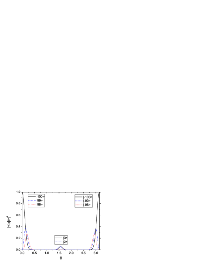
Figure 4: Variation of $|\langle\alpha|l\rangle|^{2}$ with $\theta$ for $L=100$, where $|\alpha\rangle$ is the coherent state in Eq. (7). For the three curves on the left, $l=100$ (solid curve), 99 (dashed curve) and 98 (dotted curve), respectively. For the three on the right, $l=-100,-99$ and -98, respectively. For the two in the middle, $l=0$ and 2, respectively.

In Fig. 3, we show fidelity decay at different values of $K$ corresponding to the same fixed time $t$. For $\sigma=0.01$ shown in the upper panel, at $t=1000$ the fidelity of the two Fock states $|L\rangle$ and $|-L\rangle$ is much higher than that of the other three Fock states for $K$ between 0.5 and 3. With increasing the perturbation strength $\sigma$, the fidelity at this time becomes smaller. For $\sigma=0.04$ shown in the lower panel, $M(1000)$ of $|-L\rangle$ is already small, while $M(1000)$ of $|L\rangle$ is still high within some windows of $K$. This is because the fidelity of $|-L\rangle$ decays faster than that of $|L\rangle$ (see Fig. 1 and discussions in a previous paragraph).

In quantum regular systems, the fidelity of initial coherent states is known to have initial Gaussian decay PZ02 . Hence, it is natural to check the relationship between the Fock states and the coherent states generated by generators of the group SU(2). A SU(2) coherent state $|\alpha\rangle$ centered at a point in the sphere with polar angle $\theta$ and azimuthal angle $\phi$ is given by Perelomov ; ZFG90

$$|\alpha\rangle\equiv e^{\alpha^{*}\hat{L}_{+}-\alpha\hat{L}_{-}}|-L\rangle,\ \ \text{with}\ \alpha=\frac{\pi-\theta}{2}e^{-\mathrm{i}\phi}.$$ (7)

The state $|-L\rangle$ is a coherent state with $\alpha=0$. To see the relation of other Fock states to coherent states, one can expand $|\alpha\rangle$ in the Fock states

$$|\alpha\rangle=\sum_{l=-L}^{L}\frac{(z^{*})^{l+L}}{(1+zz^{*})^{L}}\left[\frac{(2L)!}{(L+l)!(L-l)!}\right]^{1/2}|l\rangle,$$ (8)

where $z=-e^{-i\phi}\cot(\theta/2)$. This gives

$$|\langle\alpha|l\rangle|^{2}=\frac{|z|^{2(l+L)}}{(1+|z|^{2})^{2L}}\left[\frac{(2L)!}{(L+l)!(L-l)!}\right].$$ (9)

Considering the limit $|z|\to\infty$, it is easy to check that $|L\rangle$ is also a coherent state. Other Fock states are not coherent states; some examples are shown in Fig. 4.

One may expect that, since the two Fock states $|L\rangle$ and $|-L\rangle$ are coherent states, the initial slow Gaussian decay of their fidelity, as shown in Fig. 1, might be explained quantitatively by making use to results given in Ref. PZ02 . However, detailed analysis show that the situation here is more complex. Indeed, in the derivation of Gaussian decay given in Ref. PZ02 , a property of coherent states is made use of, namely, a Gaussian form of the expansion of a coherent state in the basis of Fock states. This property is possessed by most of the coherent states, but the two states $|L\rangle$ and $|-L\rangle$ are themselves Fock states. If one tries to use a $\delta$-function for the expansion, going along the line of Ref. PZ02 , it is found that their fidelity has a decay rate which is equal to zero. Hence, this approach can not explain quantitatively the initial Gaussian decay of the fidelity of the two states $|L\rangle$ and $|-L\rangle$. But, it indeed gives a qualitative explanation to the fact that the decay is slow.

IV Fidelity for different initial states

In practical situations, experimentally prepared initial states are usually not exactly the same as the expected ones. Hence, in addition to perturbation, one should also consider small change in the initial state in the study of fidelity, i.e., considering fidelity of a more general form than that in given Eq. (1). In this section, we consider such a more general fidelity and use it in the study of the stability of Fock states.

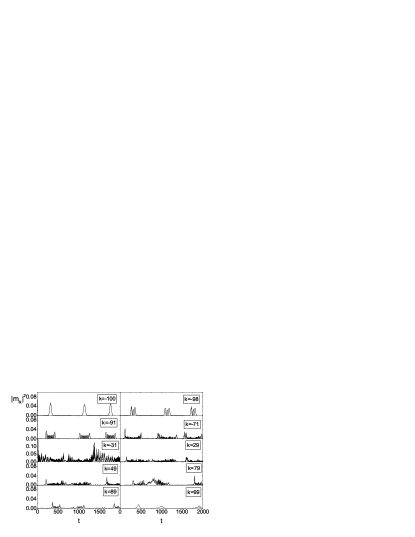
Figure 5: Variation of $|m_{lk}(t)|^{2}$ with t for $l=-31$. It has relatively regular peaks when $|k|$ is close to $L$. Parameters are $L=100,K=2,g_{c}=0.17$, for which the classical counterpart has regular motion, and $\sigma=0.5$.

IV.1 Fidelity for different initial Fock states

Suppose the expected initial state is a Fock state $|k\rangle$, while what is really prepared is the state

$$|\Psi_{0}\rangle=\sum_{l}C_{l}|l\rangle$$ (10)

with $|C_{k}|$ close to but smaller than one. The expected state at time $t$ is the time evolution of $|k\rangle$ under $H_{0}$, while the real state is the time evolution of $|\Psi_{0}\rangle$ under $H$. Hence, one should consider the following more general form of the fidelity amplitude (see Ref. nc-book ),

$$f(t)=\langle\Psi_{0}|e^{iHt}e^{-iH_{0}t}|k\rangle=\sum_{l}C_{l}^{*}m_{lk}(t),$$

where

$$m_{lk}(t)=\langle l|e^{iHt}e^{-iH_{0}t}|k\rangle.$$ (11)

The quantity $m_{lk}(t)$ can be regarded as a generalized echo, from an initial state $|k\rangle$ to a final state $|l\rangle$. Its absolute value square, $M_{lk}(t)\equiv|m_{lk}(t)|^{2}$ gives the probability for the final state to be found in $|l\rangle$, if the initial state is $|k\rangle$ and the dynamics is governed by $H_{0}$ for the first time interval $t$ and by $(-H)$ for the second interval with the same length. For $k=l$, $m_{lk}(t)$ is just the fidelity amplitude in Eq. (1). In this section, we are more interested in the case of $k\neq l$, for which $|m_{lk}(0)|^{2}=0$.

For a quantum regular system $H_{0}$, $M_{lk}(t)$ of $k\neq l$ may be considerably large within some time windows, due to the peculiarity of integrability. [If $H_{0}$ is a quantum chaotic system, $M_{lk}(t)$ usually approaches its saturation value soon and fluctuates around the saturation value.]

We would like to mention that the quantity $m_{lk}(t)$ also appears, when one considers the difference between the expectation values of an arbitrary observable $A$ for the same initial state under two slightly different Hamiltonians. Indeed, consider an initial state $|k\rangle$ and the expectation values of $A$ in the two systems

$$A_{kk}^{H_{0}}(t)\equiv\langle k|e^{iH_{0}t}Ae^{-iH_{0}t}|k\rangle,$$ (12)

$$A_{kk}^{H}(t)\equiv\langle k|e^{iHt}Ae^{-iHt}|k\rangle.$$ (13)

Inserting the identity operator $\sum_{l}e^{-iH_{0}t}|l\rangle\langle l|e^{iH_{0}t}$ in Eq. (13) before and after the operator $A$, we obtain

$$A_{kk}^{H}(t)-A_{kk}^{H_{0}}(t)={\sum_{ll^{\prime}}}^{\prime}m_{kl}(t)m_{kl^{\prime}}^{*}(t)A_{ll^{\prime}}^{H_{0}}(t),$$ (14)

where the prime over the sum implies that $l=k$ and $l^{\prime}=k$ can not hold at the same time and

$$A_{ll^{\prime}}^{H_{0}}(t)\equiv\langle l|e^{iH_{0}t}Ae^{-iH_{0}t}|l^{\prime}\rangle$$ (15)

is a quantity given in the system $H_{0}$.

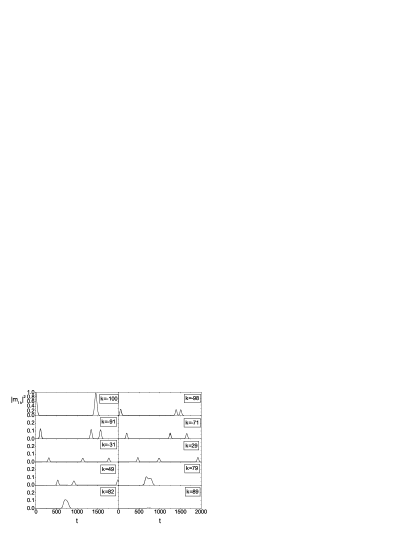
Figure 6: Same as in Fig.5 for $l=-L=-100$.

IV.2 Numerical investigation

Now we study the behavior of the quantity $M_{lk}(t)$ in the two-component BEC system discussed above. As shown in Sec. III, for some initial times the two Fock states $|L\rangle$ and $|-L\rangle$ are more stable than other Fock states $|l\rangle$ with $|l|$ not close to $L$, in the sense that the former’s fidelity is higher than the latter’s. In this section, we show that our numerical investigations in the quantity $M_{lk}(t)$ give consistent results. Specifically, $M_{lk}(t)$ with either $|l|$ or $|k|$ close to $L$ behave more regularly than those with both $|l|$ and $|k|$ far from $L$.

Let us first consider $M_{lk}(t)$ with $|l|$ far from $L$. An example is given in Fig. 5, which shows variation of $M_{lk}(t)$ with time $t$ for $L=100$, $l=-31$, and $k$ from -100 to 99. It shows that for $k$ close to $-L$, $M_{lk}(t)$ has quite regular peaks, and with increasing $k$ from $-L$ to $0$, the peaks become more and more irregular. Similarly, for $k$ decreasing from $L$ to 0, the peaks of $M_{lk}(t)$ also becomes more and more irregular.

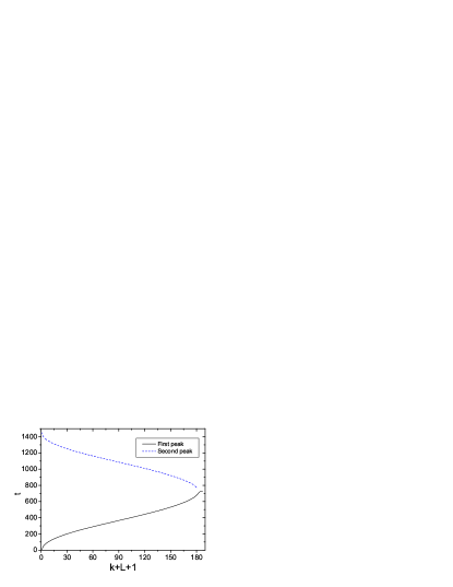
Figure 7: Variation with $k$ for the times corresponding to the centers of the first and second peaks of $|m_{lk}(t)|^{2}$ shown in Fig. 6.

On the other hand, for $l=-L=-100$, $M_{lk}(t)$ behaves regularly for all the values of $k$, as shown in Fig. 6. Here, the basic feature is that for each value of $k$, $M_{lk}(t)$ is considerably large only within some time intervals. Specifically, for $k=-100$, $M_{lk}(t)=1$ at $t=0$ as a trivial result of $k=l$, then, it decays and remains small until $t\simeq 1370$ after which there is a revival, forming a second peak centered at $t\simeq 1450$. The second peak of $M_{lk}(t)$ of $k=-100$ splits into two peaks when $k=-98$, hence, $M_{lk}(t)$ has three peaks for $k=-98$. Interestingly, with further increasing $k$, the first peak of $M_{lk}(t)$ moves to the right while the second peak moves to the left. The two peaks meet at a value of $k$ a little smaller than 79. In Fig. 7, we show variation of the times corresponding to the centers of the first and second peaks with increasing $k$.

The structure of the peaks shown in Fig. 6 suggests that at each fixed time $t$, $|M_{lk}(t)|$ of $l=-L$ may be concentrated in a relatively small region of $k$. Indeed, this is confirmed by our further numerical simulations. We have calculated the quantity

$$S_{k}(l,t)=\sum_{k^{\prime}\leq k}M_{lk^{\prime}}(t),$$ (16)

which gives the total probability for $k^{\prime}\leq k$. Examples for some fixed times are given in Fig. 8, which shows that $|M_{lk}(t)|$ of $l=-L$ is indeed concentrated in a relatively narrow region of $k$ for each time.

V Conclusions

By numerical simulations, we have studied quantum Loschmidt echo or fidelity decay of initial Fock states in a two-component BEC system, whose classical counterpart has regular motion. Our results show that, for some initial times, initial Fock states with all the atoms in one component of the BEC are more stable than Fock states with atoms distributed in the two components. This implies that one-component BEC might be more stable than two-component BEC.

We have further investigated this issue by considering a more general form of the fidelity, i.e., fidelity for different initial states. Numerical computations of the general fidelity show consistent results, namely, initial Fock states with all the atoms in the same component behave more regularly than other Fock states.

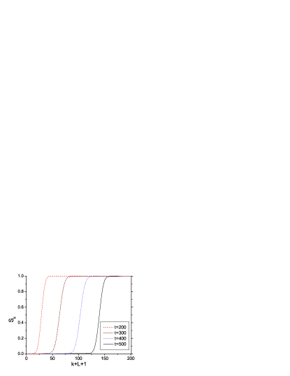
Figure 8: Values of $S_{k}=\sum_{k^{\prime}\leq k}M_{lk^{\prime}}(t)$ for $l=-L$. Parameters are the same as in Fig.5. It shows that at each of the times, $M_{lk}(t)$ is concentrated in a small region of $k$.

Appendix A An experimental scheme for measuring fidelity

In this appendix, we discuss in detail an experimental scheme for measuring fidelity decay in a BEC system, which is briefly sketched in the last section of Ref. pra05-bec , and give an explicit expression of the fidelity in terms of measurable quantities.

Experimental schemes for measuring fidelity have been discussed by several groups and basically three types of schemes have been proposed GPSZ06 . In the first type of scheme, a quantum system is considered, which is composed of two subsystems (or has two degrees of freedom) GCZ97 ; HBSSR05 ; WB06 ; PD07 . The system is assumed to have a time evolution such that the fidelity of the first subsystem is given by the reduced density matrix of the second subsystem GPSS04 ; QSLZS06 . Then, measuring properties of the second subsystem which can be small, fidelity of the first subsystem which may be large can be obtained. This scheme is adopted in the experiments in Ref. AKD03 ; REPNL05 . To be specific, one may consider a Hilbert space which is the direct product of a two-dimensional subspace with basis states $|1\rangle$ and $|2\rangle$ and a second subspace for state vectors $|\psi\rangle$. The Hamiltonian has the form $H=H_{1}|1\rangle\langle 1|+H_{2}|2\rangle\langle 2|$, where $H_{1}$ and $H_{2}$ act in the second subspace only. For an initial state $|\Psi(0)\rangle=(|1\rangle+|2\rangle)|\psi_{0}\rangle/\sqrt{2}$, the state at time $t$ is $|\Psi(t)\rangle=\frac{1}{\sqrt{2}}\left(e^{-iH_{1}t}|\psi_{0}\rangle|1\rangle+e^{-iH_{2}t}|\psi_{0}\rangle|2\rangle\right)$ . Then, the fidelity amplitude $\langle\psi_{0}|e^{iH_{2}t}e^{-iH_{1}t}|\psi_{0}\rangle$ in the second subspace is related to an off-diagonal element of the reduced density matrix in the first subspace.

In the second type of scheme, a special kind of system is considered, for which the time evolution can be such controlled that the system evolves under $H_{0}$ for a time period $t$, then, evolves under $(-H_{0}-\epsilon V)$ for a second period $t$. The fidelity is then just the survival probability, i.e., the probability for the final state to be found in the initial state. In the third type, classical waves are employed, which evolves according to a dynamical law mathematically equivalent to Schrödinger equation SSGS05 .

Now we discuss the scheme briefly mentioned in Ref. pra05-bec . We propose to use a setup similar to that used in Ref. ketterle . Consider a BEC (e.g. ${}^{87}Rb$) which is optically cooled and trapped, then, transferred into a double-well potential. The double-well potential can be created by deforming a single-well optical trap into a double-well potential with linearly increasing the frequency difference between the rf signals ketterle . Near-resonant coupling fields are applied to the BEC in the two wells with slight difference in strength. Finally, simultaneously switching off all the external fields and letting the BEC expand freely, interference pattern of the BEC can be observed. The wells should be deep, such that the total density remains approximately a constant, and the atom numbers in the two wells are required nearly equal.

At the initial time $t_{0}$, suppose the state of the system is a product state $|\Psi(t_{0})\rangle=|\phi(t_{0})\rangle|\psi(t_{0})\rangle|\Phi_{p}(t_{0})\rangle,$ where $|\phi(t_{0})\rangle$ is the internal state of the atoms, e.g., with all the atoms in the same hyperfine internal state, $|\psi(t_{0})\rangle$ describes the motion of the center-of-mass degrees of freedom of the atoms, and $|\Phi_{p}(t_{0})\rangle$ represents the field forming the optical trap. We assume that the field of the optical trap is not entangled with the BEC in the experimental process and shall omit the term $|\Phi_{p}(t)\rangle$.

From time $t_{0}$ to $t_{1}$, the potential of the optical trap is deformed into a double-well potential. If the internal state of the atoms is not influenced in this process, at $t=t_{1}$, one has $|\Psi(t_{1})\rangle=|\phi(t_{1})\rangle\left[|\psi_{1}({\bf R}_{1},t_{1})\rangle+|\psi_{2}({\bf R}_{2},t_{1})\rangle\right],$ where ${\bf R}_{1}$ and ${\bf R}_{2}$ indicate spatial locations of the two wells, respectively.

From time $t_{1}$ to $t_{2}$, near-resonant coupling fields can be applied to the condensates to couple the two hyperfine states. The coupling fields have a slight difference in strength in the two wells. We assume that the near-resonant coupling fields can be treated as classical fields and do not induce tunnelling between the two wells. The internal states of the condensate in the two wells will then evolve differently. Thus, for $t\in(t_{1},t_{2})$,

$$|\Psi(t)\rangle=|\phi_{1}(t)\rangle|\psi_{1}({\bf R}_{1},t)\rangle+|\phi_{2}(t)\rangle|\psi_{2}({\bf R}_{2},t)\rangle.$$ (17)

In the case that the internal degrees of freedom are not coupled to the center-of-mass degrees of freedom, $|\phi_{j}(t)\rangle$ has unitary time evolution

$$|\phi_{j}(t)\rangle=U_{j}(t_{1},t)|\phi(t_{1})\rangle,$$ (18)

with $j=1,2$ indicating the two wells. The internal state can be expanded in the Fock states $|l\rangle$,

$$|\phi_{j}(t)\rangle=\sum_{l}d_{l}^{(j)}(t)|l\rangle.$$ (19)

At $t=t_{2}$, one can simultaneously switch off all the external fields and let the two clouds of BEC expand freely. For $t>t_{2}$, Eqs. (17) and (19) are still valid. Substituting Eq. (19) into Eq. (17), one has

$$|\Psi(t)\rangle=\sum_{l}\left[d_{l}^{(1)}(t)|\psi_{1}({\bf R}_{1},t)\rangle+d_{l}^{(2)}(t)|\psi_{2}({\bf R}_{2},t)\rangle\right]|l\rangle.\ \$$ (20)

Suppose the single particle states for $|\psi_{1}({\bf R}_{1},t)\rangle$ and $|\psi_{2}({\bf R}_{2},t)\rangle$ are $\chi_{1}({\bf x},t)$ and $\chi_{2}({\bf x},t)$, respectively. Then, the probability of finding a particle at a position ${\bf x}$ is

$$P({\bf x},t)=|\chi_{1}|^{2}+|\chi_{2}|^{2}+2{\rm Re}\left[\widetilde{f}(t)\chi_{1}\chi_{2}^{*}\right],$$ (21)

where $\widetilde{f}(t)\equiv\sum_{l}d_{l}^{(1)}(t){d_{l}^{(2)}}^{*}(t)$.

Making use of Eqs. (18) and (19), it is seen that

$$\widetilde{f}(t)=\langle\phi(t_{1})|U_{2}^{{\dagger}}(t_{1},t)U_{1}(t_{1},t)|\phi(t_{1})\rangle,$$ (22)

which is a fidelity amplitude. Since there is no coupling field beyond $t_{2}$, $U_{1}(t_{2},t)=U_{2}(t_{2},t)$ and, as a result, $\widetilde{f}(t)=\widetilde{f}(t_{2})$ for $t>t_{2}$. Then, Eq. (21) can be written as

$$2|\widetilde{f}(t_{2})|{\rm Re}\left[e^{i\theta_{f}(t_{2})}\chi_{1}\chi_{2}^{*}\right]=P({\bf x},t)-|\chi_{1}|^{2}-|\chi_{2}|^{2},$$ (23)

where $\theta_{f}(t_{2})$ is the phase of $\widetilde{f}(t_{2})$. Therefore, the value of $|\widetilde{f}(t_{2})|$ can be obtained by measuring the interference pattern of the two expanding clouds of BEC.

References

- (1) M. D. Lukin, Rev. Mod. Phys. 75, 457 (2003).
- (2) M. H. Anderson, et al, Science 269, 198 (1995); K.Davis, et al, Phys. Rev. Lett. 75, 3969 (1995); C.C.Bradley, et al, Phys. Rev. Lett. 75, 1687 (1995).
- (3) S. Sinha and Y. Castin, Phys. Rev. Lett. 87, 190402 (2001); P. Buonsante, R. Franzosi, and V. Penna,Phys. Rev. Lett. 90, 050404 (2003).
- (4) L. J. Garay, J. R. Anglin, J. I. Cirac, and P. Zoller, Phys. Rev. Lett. 85, 4643 (2000).
- (5) V. V. Konotop and M. Salerno,Phys. Rev. A 65, 021602 (2002); L. Salasnich, A. Parola, and L. Reatto, Phys. Rev. Lett. 91, 080405 (2003); L. D. Carr and J. Brand,Phys. Rev. Lett. 92, 040401 (2004).
- (6) P. Buonsante, P. G. Kevrekidis, V. Penna, and A. Vezzani, Phys. Rev. E 75, 016212 (2007).
- (7) J. R. Anglin and A. Vardi,Phys. Rev. A 64, 013605 (2001); V. A. Yurovsky, Phys. Rev. A 65, 033605 (2002); G. P. Berman, A. Smerzi, and A. R. Bishop,Phys. Rev. Lett. 88, 120402 (2002).
- (8) Jie Liu, Biao Wu, and Qian Niu Phys. Rev. Lett. 90, 170404 (2003); C. Zhang, J. Liu, M. G. Raizen, and Q. Niu, Phys. Rev. Lett. 92, 054101 (2004); C. Zhang, J. Liu, M. G. Raizen, and Q. Niu Phys. Rev. Lett. 93, 074101 (2004).
- (9) Jie Liu, Wenge Wang, Chuanwei Zhang, Qian Niu, and Baowen Li, Phys. Rev. A, 72, 063623 (2005); Phys. Lett. A, 353, 216 (2006).
- (10) J. D. Bodyfelt, M. Hiller, and T. Kottos, Europhys. Lett. 78, 50003 (2007); G. Manfredi and P.-A. Hervieux, Phys. Rev. Lett. 100, 050405 (2008).
- (11) A. Peres, Phys. Rev. A 30, 1610 (1984).
- (12) G. Benenti, G. Casati and G. Strini, Principles of Quantum Computation and Information (World Scientific, Singapore, 2004).
- (13) M.A. Nielsen and I.L. Chuang, Quantum Computation and Quantum Information (Cambridge University Press, Cambridge, 2000).
- (14) R.A. Jalabert and H.M. Pastawski, Phys. Rev. Lett. 86, 2490 (2001);
- (15) Ph. Jacquod, P.G. Silvestrov, and C.W.J. Beenakker, Phys. Rev. E 64, 055203(R) (2001).
- (16) G. Benenti and G. Casati, Phys. Rev. E 65, 066205(2002);
- (17) N. R. Cerruti and S. Tomsovic, Phys. Rev. Lett. 88, 054103 (2002); J. Phys. A 36, 3451 (2003).
- (18) T. Prosen and M. Žnidarič, J. Phys. A 35, 1455 (2002).
- (19) W. Wang and B. Li, Phys. Rev. E 66, 056208 (2002); W.Wang, G.Casati, and B.Li, ibid. 69, 025201(R)(2004); W. Wang and B. Li, ibid. 71, 066203 (2005); W.Wang, G. Casati, B. Li, and T. Prosen, ibid. 71, 037202 (2005).
- (20) J. Vaníček and E.J. Heller, Phys. Rev. E 68, 056208 (2003).
- (21) P.G. Silvestrov, J. Tworzydło, and C.W.J. Beenakker, Phys. Rev. E 67, 025204(R) (2003).
- (22) J. Vaníček, Phys. Rev. E 70, 055201(R) (2004); 73, 046204 (2006); e-print quant-ph/0410205.
- (23) T. Gorin, T. Prosen, T.H. Seligman, and M. Žnidarič, Phys. Rep. 435, 33 (2006) (quant-ph/0607050).
- (24) T. Prosen and M. Žnidarič, New J. Phys. 5, 109 (2003).
- (25) Ph. Jacquod, I. Adagideli, and C.W.J. Beenakker, Europhys. Lett. 61, 729 (2003).
- (26) R. Sankaranarayanan and A. Lakshminarayan, Phys. Rev. E 68, 036216 (2003).
- (27) Y.S. Weinstein and C.S. Hellberg, Phys. Rev. E 71, 016209 (2005).
- (28) M. Combescure, J. Phys. A 38, 2635, 2005; M. Combescure, J. Mat. Phys. 47, 032102 (2006); M. Combescure and D. Robert, quant-ph/0510151.
- (29) F. Haug, M. Bienert, W. P. Schleich, T. H. Seligman, and M. G. Raizen, Phys. Rev. A 71, 043803 (2005).
- (30) S. Wimberger and A. Buchleitner, J. Phys. B 39, L145 (2006).
- (31) W. Wang, G. Casati, and B. Li, Phys. Rev. E 75, 016201 (2007).
- (32) M. R. Matthews, B. P. Anderson, P. C. Haljan, D. S. Hall, M. J. Holland, J. E. Williams, C. E. Wieman, and E. A. Cornell, Phys. Rev. Lett. 83, 3358 (1999).
- (33) L.You, Phys. Rev. Lett. 90, 030402 (2003); M.Zhang and L.You, Phys. Rev. Lett. 91, 230404 (2003);A.P.Hines, R.H.McKenzie, and G.J.Milburn, Phys. Rev. A 67, 013609(2003).
- (34) A.J.Leggett, Rev. Mod. Phys. 73, 307 (2001).
- (35) A. Vardi and J. R. Anglin, Phys. Rev. Lett. 86, 568 (2001).
- (36) F. Haake, Quantum Signature of Chaos (Springer-Verlag, New York, 2000).
- (37) A. Perelomov, Generalized Coherent States and Their Applications (Springer-Verlag, Berlin, 1986).
- (38) W.-M. Zhang, D. H. Feng, and R. Gilmore, Rev. Mod. Phys. 62, 867 (1990).
- (39) S.A. Gardiner, J.I. Cirac, and P. Zoller, Phys. Rev. Lett. 79, 4790 (1997).
- (40) E.N. Pozzo and D. Domínguez, Phys. Rev. Lett. 98, 057006 (2007).
- (41) T. Gorin, T. Prosen, T.H. Seligman, and W.T. Strunz, Phys. Rev. A 70, 042105 (2004).
- (42) H.T. Quan, Z. Song, X.F. Liu, P. Zanardi, and C.P. Sun, Phys. Rev. Lett. 96, 140604 (2006).
- (43) M.F. Andersen, A. Kaplan, and N. Davidson, Phys. Rev. Lett. 90, 023001 (2003).
- (44) C.A. Ryan, J. Emerson, D. Poulin, C. Negrevergne, and R. Laflamme, Phys. Rev. Lett. 95, 250502 (2005).
- (45) R. Schäfer, H.-J. Stöckmann, T. Gorin, and T.H. Seligman, Phys. Rev. Lett. 95, 184102 (2005).
- (46) Y. Shin, M. Saba, T. A. Pasquini, W. Ketterle, D. E. Pritchard, and A. E. Leanhardt , Phys. Rev. Lett. 92, 050405 (2004).