Quantum Symmetries for Exceptional ${\rm SU}(4)$ Modular Invariants

Quantum Symmetries for Exceptional $\boldsymbol{{\rm SU}(4)}$ Modular Invariants Associated with Conformal Embeddings

Robert COQUEREAUX and Gil SCHIEBER

R. Coquereaux and G. Schieber Centre de Physique Théorique (CPT), Luminy, Marseille, France

coque@cpt.univ-mrs.fr, schieber@cpt.univ-mrs.fr

Received December 24, 2008, in final form March 31, 2009; Published online April 12, 2009

Three exceptional modular invariants of ${\rm SU}(4)$ exist at levels $4$, $6$ and $8$. They can be obtained from appropriate conformal embeddings and the corresponding graphs have self-fusion. From these embeddings, or from their associated modular invariants, we determine the algebras of quantum symmetries, obtain their generators, and, as a by-product, recover the known graphs ${\mathcal{E}}_{4}$, ${\mathcal{E}}_{6}$ and ${\mathcal{E}}_{8}$ describing exceptional quantum subgroups of type ${\rm SU}(4)$. We also obtain characteristic numbers (quantum cardinalities, dimensions) for each of them and for their associated quantum groupoïds.

quantum symmetries; modular invariance; conformal field theories

81R50; 16W30; 18D10

Foreword

General presentation. A classification of ${\rm SU}(4)$ graphs associated with WZW models, or “quantum graphs” for short, was presented by A. Ocneanu in [32] and claimed to be completed. These graphs generalize the ADE Dynkin diagrams that classify the ${\rm SU}(2)$ models [8], and the Di Francesco–Zuber diagrams that classify the ${\rm SU}(3)$ models [14]. They describe modules over a ring of irreducible representations of quantum ${\rm SU}(4)$ at roots of unity. A particular partition function associated with each of those quantum graphs is modular invariant.

According to [32], the ${\rm SU}(4)$ family includes the ${\mathcal{A}}_{k}$ series (describing fusion algebras) and their conjugates for all $k$, two kinds of orbifolds, the ${\mathcal{D}}^{(2)}_{k}=\mathcal{A}_{k}/2$ series for all $k$ (with self-fusion when $k$ is even), and members of the ${\mathcal{D}}^{(4)}_{k}=\mathcal{A}_{k}/4$ series when $k$ is even (with self-fusion when $k$ is divisible by 8), together with their conjugates. The orbifolds are constructed by using the $Z_{4}$ action on weigths generated by ${\epsilon\{\lambda_{1},\lambda_{2},\lambda_{3}\}=\{k-\lambda_{1}-\lambda_{2}-\lambda_{3},\lambda_{1},\lambda_{2}\}}$ or the $Z_{2}$ action generated by $\epsilon^{2}$. The ${\rm SU}(4)$ family also includes an exceptional case, ${\mathcal{D}^{(4)t}_{8}}$, without self-fusion (a generalization of $E_{7}$), and three exceptional quantum graphs with self-fusion, at levels $4$, $6$ and $8$, denoted ${\mathcal{E}}_{4}$, ${\mathcal{E}}_{6}$ and ${\mathcal{E}}_{8}$, together with one exceptional module for each of the last two. The modular invariant partition functions associated with ${\mathcal{E}}_{4}$, ${\mathcal{E}}_{6}$ and ${\mathcal{E}}_{8}$ can be obtained from appropriate conformal embeddings, namely from ${\rm SU}(4)$ level $4$ in ${\rm Spin}(15)$, from ${\rm SU}(4)$ level $6$ in ${\rm SU}(10)$, and from ${\rm SU}(4)$ level 8 in ${\rm Spin}(20)$. There exists also a conformal embedding of ${\rm SU}(4)$, at level 2, in ${\rm SU}(6)$, but this gives rise to $\mathcal{D}^{(2)}_{2}=\mathcal{A}_{2}/2$, the first member of the ${\mathcal{D}}^{(2)}_{k}$ series. This exhausts the list of conformal embeddings of ${\rm SU}(4)$. The other ${\rm SU}(4)$ quantum graphs, besides the ${\mathcal{A}}_{k}$, can either be obtained as modules over the exceptional ones, or are associated (possibly using conjugations) with non-simple conformal embeddings followed by contraction, ${\rm SU}(4)$ appearing only as a direct summand of the embedded algebra.

Vertices $a,b,\ldots$ of a chosen quantum graph (denoted generically by ${\mathcal{E}}_{k}$) describe boundary conditions for a WZW conformal field theory specified by ${\rm SU}(4)_{k}$. These irreducible objects span a vector space which is a module over the fusion algebra, itself spanned, as a linear space, by the vertices $m,n,\ldots$ of the graph ${\mathcal{A}}_{k}({\rm SU}(4))$, or ${\mathcal{A}}_{k}$ for short since ${\rm SU}(4)$ is chosen once and for all, the truncated Weyl chamber at level $k$ (a Weyl alcove). Vertices of ${\mathcal{A}}_{k}$ can be understood as integrable irreducible highest weight representations of the affine Lie algebra $\widehat{su}(4)$ at level $k$ or as irreducible representations with non-zero $q$-trace of the quantum group ${\rm SU}(4)_{q}$ at the root of unity $q=\exp(i\pi/(k+g))$, $g$ being the dual Coxeter number (for ${\rm SU}(4)$, $g=4$). Edges of ${\mathcal{E}}_{k}$ describe action of the fundamental representations of ${\rm SU}(4)$, the generators of ${\mathcal{A}}_{k}$.

To every quantum graph one associates an algebra of quantum symmetries ${\mathcal{O}}$, along the lines described in [31]. Its vertices $x,y,\ldots$ can be understood, in the interpretation of [35], as describing the same BCFT theory but with defects labelled by $x$. To every fundamental representation ($3$ of them for ${\rm SU}(4)$) one associates two generators of ${\mathcal{O}}$, respectively called “left” and “right”. Multiplication by these generators is described by a graph, called the Ocneanu graph. Its vertices span the algebra ${\mathcal{O}}$ as a linear space, and its edges describe multiplication by the left and right fundamental generators (we have $6=2\times 3$ types of edges for ${\rm SU}(4)$).

The exceptional modular invariants at level $4$ and $6$ were found by [40, 3], and at level $8$ by [2]. The corresponding quantum graphs ${\mathcal{E}}_{4}$, ${\mathcal{E}}_{6}$ and ${\mathcal{E}}_{8}$ were respectively obtained by [36, 37, 32]. There are several techniques to determine quantum graphs. One of them, probably the most powerful but involving rather heavy calculations, is to obtain the quantum graph associated with a modular invariant as a by-product of the determination of its algebra of quantum symmetries. This requires in particular the solution of the so-called modular splitting equation, which is a huge collection of equations between matrices with non-negative integral entries, involving the known fusion algebra, the chosen modular invariant, and expressing the fact that ${\mathcal{O}}$ is a bi-module over ${\mathcal{A}}_{k}$. Because of the heaviness of the calculation, a simplified method using only the first line of the modular invariant matrix was used in [32] to achieve this goal, namely the determination of ${\rm SU}(4)$ quantum graphs (some of them, already mentioned, were already known) but the algebra of quantum symmetries was not obtained in all cases. To our knowledge, for exceptional modular invariants of ${\rm SU}(4)$ at levels $4$, $6$ and $8$, the full modular splitting system had not been solved, the full torus structure had not been obtained, and the graph of quantum symmetries was not known. This is what we did. We have recovered in particular the structure of the already known quantum graphs; they now appear, together with their modules, as components of their respective Ocneanu graphs.

Categorical description. Category theory offers a synthetic presentation of the whole subject and we present it here in a few lines, for the benefice of those readers who may find appealing such a description. However, it will not be used in the body of our article. The starting point is the fusion category ${\mathcal{A}}_{k}$ associated with a Lie group $K$. This modular category, both monoidal and ribbon, can be defined either in terms of representation theory of an affine Lie algebra (simple objects are highest weight integrable irreducible representations), or in terms of representation theory of a quantum group at roots of unity (simple objects are irreducible representations of non-vanishing quantum dimension). In the case of ${\rm SU}(2)$, we refer to the description given in [34, 17]. One should keep in mind the distinction between this category (with its objects and morphisms), its Grothendieck ring (the fusion ring), and the graph describing multiplication by its generators, but they are denoted by the same symbol. The next ingredient is an additive category ${\mathcal{E}}_{k}$, not modular usually, on which the previous one, ${\mathcal{A}}_{k}$, acts. In general this module-category ${\mathcal{E}}_{k}$ has no-self-fusion (no compatible monoidal structure) but in the cases studied in the present paper, it does. Again, the category itself, its Grothendieck group, and the graph (here called McKay graph) describing the action of generators of ${\mathcal{A}}_{k}$ are denoted by the same symbol. The last ingredient is the centralizer (or dual) category ${\mathcal{O}}={\mathcal{O}}({\mathcal{E}}_{k})$ of ${\mathcal{E}}_{k}$ with respect to the action of ${\mathcal{A}}_{k}$. It is monoidal and comes with its own ring (the algebra of quantum symmetries) and graph (the Ocneanu graph). One way to obtain a realization of this collection of data is to construct a finite dimensional weak bialgebra ${\mathcal{B}}$, which should be such that ${\mathcal{A}}_{k}$ can be realized as ${\rm Rep}({\mathcal{B}})$, and also such that ${\mathcal{O}}$ can be realized as ${\rm Rep}({\widehat{\mathcal{B}}})$, where $\widehat{\mathcal{B}}$ is the dual of ${\mathcal{B}}$. These two algebras are finite dimensional, actually semisimple in our case, and one algebra structure (say $\widehat{\mathcal{B}}$) can be traded against a coalgebra structure on its dual. ${\mathcal{B}}$ is a weak bialgebra, not a bialgebra, because $\Delta\mbox{\rm 1}\hskip-2.8pt\mbox{\rm l}\neq\mbox{\rm 1}\hskip-2.8pt\mbox{\rm l}\otimes\mbox{\rm 1}\hskip-2.8pt\mbox{\rm l}$, the coproduct in ${\mathcal{B}}$ being $\Delta$, and 1l its unit. ${\mathcal{B}}$ is not only a weak bialgebra but a weak Hopf algebra: one can define an antipode, with the expected properties.

Remark 0.1.

Given a graph defining a module over a fusion ring ${\mathcal{A}}_{k}$ for some Lie group $K$, the question is to know if it is a “good graph”, i.e., if the corresponding module-category indeed exists. Using A. Ocneanu’s terminology [32], this will be the case if and only if one can associate, in a coherent manner, a complex number to each triangle of the graph (when the rank of $K$ is $\geq 2$): this defines, up to some kind of gauge choice, a self-connection on the set of triangular cells. Here, “coherent manner” means that there are two compatibility equations, respectively nicknamed the small and large pocket equations, that this self-connection should obey. These equations reflect properties that hold for the intertwining operators of a fusion category, they are sometimes called “compatibility equations for Kuperberg spiders” (see [27]). The point is that exhibiting a module over a fusion ring does not necessarily entail existence of an underlying theory: when the graph (describing the module structure) does not admit any self-connection in the above sense, it should be rejected; another way to express the same thing is to say that a particular family of $6j$ symbols, expected to obey appropriate equations, fails to be found. Such features are not going to be discussed further in the present paper.

Historical remarks concerning $\boldsymbol{{\mathcal{E}}_{8}({\rm SU}(4))}$. Not all conformal embeddings $K\subset G$ correspond to isotropy-irreducible pairs and not all isotropy-irreducible homogeneous spaces define conformal embeddings. However, it is a known fact that most isotropy irreducible spaces $G/K$ (given in [42]) indeed define conformal embeddings. This is actually so in all examples studied here, and in particular for the ${\rm SU}(4)\subset{\rm Spin}(20)$ case which can also be recognized as the smallest member ($n=1)$ of a $D_{2n+1}\subset D_{(n+1)(4n+1)}$ family of conformal embeddings appearing on table $4$ of the standard reference [4], and on table II(a) of the standard reference [39], since ${\rm SU}(4)\simeq{\rm Spin}(6)$. This embedding, which is “special” (i.e., non regular: unequal ranks and Dynkin index not equal to $1$), does not seem to be quoted in other standard references on conformal embeddings (for instance [25, 28, 41]), although it is explicitly mentioned in [2] and although its rank-level dual is indirectly used in case 18 of [38], or in [44]. The corresponding ${\rm SU}(4)$ modular invariant was later recovered by [32], using arithmetical methods, and used to determine the ${\mathcal{E}}_{8}({\rm SU}(4))$ quantum graph, but since the existence of an associated conformal embedding had slipped into oblivion, it was incorrectly stated that this particular example could not be obtained from conformal embedding considerations.

Structure of the article. The technique relating modular invariants to conformal embeddings is standard [13] but the results concerning ${\rm SU}(4)$ are either scattered in the literature, or unpublished; for this reason, we devote the main part of the first section to it. In the same section, we obtain characteristic numbers (quantum cardinality, quantum dimensions etc.) for the ${\mathcal{E}}_{k}$ graphs. In the second section, after a description of the structures at hand and a general presentation of our method of resolution, we solve, in a first step, for the three exceptional cases ${\mathcal{E}}_{4}$, ${\mathcal{E}}_{6}$ and ${\mathcal{E}}_{8}$ of the ${\rm SU}(4)$ family, the full modular splitting equation that determines the corresponding set of toric matrices (generalized partition functions) and, in a second step, the general intertwining equations that determine the structure of the generators of the algebra of quantum symmetries. The size of calculations involved in this part is huge (quite intensive computer help was required) and, for reasons of size, we can only present part of our results. On the other hand, each case being exceptional, there are no generic formulae. For each case, we encode the structure of the algebra of quantum symmetries by displaying the Cayley graphs of multiplication by the fundamental generators, whose collection makes the Ocneanu graph. We also give a brief description of the structure of the corresponding quantum groupoïds. In the appendices, after a short description of the Kac–Peterson formula, we gather several explicit results, providing quantum dimensions for those irreducible representations of the various groups used in the text.

The interested reader may also consult the article [12] which provides more information on the general theory and gives a more complete description of the $\mathcal{E}_{4}({\rm SU}(4))$ case. Properties of quantum graphs of type ${\rm SU}(3)$ and their quantum symmetries are summarized in [11], see also [21] and references therein. Those of type ${\rm SU}(2)$ are certainly well known but many explicit results, like the explicit structure of toric matrices for exceptional diagrams, can be found in [10].

1 Conformal embeddings of $\boldsymbol{{\rm SU}(4)}$

1.1 Homogeneous spaces $\boldsymbol{G/K}$

We describe the embeddings of $K={\rm SU}(4)$ in $G={\rm Spin}(15),\,{\rm SU}(10),\,{\rm Spin}(20)$. The reduction of the adjoint representation of $G$ with respect to $K$ reads ${\rm Lie}(G)={\rm Lie}(K)\oplus T(G/K)$. The isotropy representation of $K$ on the tangent space at the origin of $G/K$ has dimension $\dim(G)-\dim(K)$. In all three cases, the space $G/K$ is isotropy irreducible (but not symmetric): the isotropy representation is real irreducible. After extension to the field of complex numbers it may stay irreducible (strong irreducibility) or not. The following are known results, already mentioned in [42].

• ${\rm SU}(4)\subset{\rm SU}(6)$. This embedding leads to the lowest member of an orbifold series (the ${\mathcal{D}}_{2}^{(2)}={\mathcal{A}}_{2}/2$ graph) and, in this paper, we are not interested in it.

• ${\rm SU}(4)\subset{\rm Spin}(15)$. Reduction of the adjoint representation of $G$ with respect to $K$ reads $[105]\mapsto[15]+[90]$. After complexification, $[90]$ is recognized as the reducible representation with highest weight $\{0,1,2\}\oplus\{2,1,0\}=[45]\oplus[\overline{45}]$ so that $G/K$ is not strongly irreducible.

• ${\rm SU}(4)\subset{\rm SU}(10)$. Reduction of the adjoint representation of $G$ with respect to $K$ reads $[99]\mapsto[15]+[84]$. After complexification, $[84]$ is recognized as the irreducible representation with highest weight $\{2,0,2\}$ so that $G/K$ is strongly irreducible.

• ${\rm SU}(4)\subset{\rm Spin}(20)$. Reduction of the adjoint representation of $G$ with respect to $K$ reads $[190]\mapsto[15]+[175]$. After complexification, $[175]$ is recognized as the irreducible representation with highest weight $\{1,2,1\}$, so that $G/K$ is strongly irreducible.

1.2 The Dynkin index of the embeddings

The Dynkin index $k$ of an embedding $K\subset G$ defined by a branching rule $\mu\mapsto\sum_{j}\alpha_{j}\nu_{j}$, where $\mu$ refers to the adjoint representation of $G$ (one of the $\nu_{j}$ on the right hand side is the adjoint representation of $K$), $\alpha_{j}$ being multiplicities, is obtained in terms of the quadratic Dynkin indices $I_{\mu}$, $I_{\nu_{j}}$ of the representations:

$$k=\sum_{j}\alpha_{j}I_{\nu_{j}}/I_{\mu}\qquad\hbox{with}\quad I_{\lambda}=\frac{\dim(\lambda)}{2\dim(K)}\langle\lambda,\lambda+2\rho\rangle.$$

Here $\rho$ is the Weyl vector and $\langle\;,\;\rangle$ is defined by the fundamental quadratic form. For the three embeddings of ${\rm SU}(4)$ that we consider, into ${\rm Spin}(15)$, ${\rm SU}(10)$ and ${\rm Spin}(20)$, one finds respectively $k=4,6,8$.

1.3 Those embeddings are conformal

An embedding $K\subset G$, for which the Dynkin index is $k$, is conformal if the following equality is satisfied:

$$\frac{\dim(K)\times k}{k+g_{K}}=\frac{\dim(G)\times 1}{1+g_{G}},$$

where $g_{K}$ and $g_{G}$ are the dual Coxeter numbers of $K$ and $G$. One denotes by $c$ the common value of these two expressions. In the framework of affine Lie algebras, $c$ is interpreted as a central charge and the numbers $k$ and $1$ denote the respective levels for the affine algebras corresponding to $K$ and $G$. The above definition, however, does not require the framework of affine Lie algebras (or of quantum groups at roots of unity) to make sense.

Using $\dim(G)=105,\,99,\,190$, for $G={\rm Spin}(15),\,{\rm SU}(10),\,{\rm Spin}(20)$, $\dim(K={\rm SU}(4))=15$ and the corresponding values for the dual Coxeter numbers $g_{G}=13,\,10,\,18$ and $g_{K}=4$, we see immediately that the above equality is obeyed, for the levels $k=4,6,8$, with central charges $c=15/2$, $c=9$, and $c=10$.

The conformal embeddings of ${\rm SU}(4)$ into ${\rm SU}(6)$, ${\rm SU}(10)$ and ${\rm Spin}(15)$ belong respectively to the series of embeddings of ${\rm SU}(N)$ into ${\rm SU}(N(N-1)/2)$, ${\rm SU}(N(N+1)/2$ and ${\rm Spin}(N^{2}-1)$, at respective levels $N-2$, $N+2$ and $N$ (provided $N$ is big enough), whereas the last one, namely ${\rm SU}(4)$ into ${\rm Spin}(20)$, is recognized as the smallest member of the ${\rm Spin}(N)\subset{\rm Spin}((2N+2)(4N+1))$ series, since ${\rm SU}(4)\simeq{\rm Spin}(6)$.

1.4 The modular invariants

Here we reduce the diagonal modular invariants of $G={\rm Spin}(15),\,{\rm SU}(10),\,{\rm Spin}(20)$, at level $k=1$, to $K={\rm SU}(4)$, at levels $k=4,6,8$, and obtain exceptional modular invariants for ${\rm SU}(4)$ at those levels. The previous section was somehow “classical” whereas this one is “quantum”. Since there is an equivalence of categories [15, 26] between the fusion category (integrable highest weight representations) of an affine algebra at some level and a category of representations with non-zero $q$-dimension for the corresponding quantum group at a root of unity determined by the level, we shall freely use both terminologies. From now on, simple objects will be called i-irreps, for short.

1.4.1 The method

• One has first to determine what i-irreps $\lambda$ appear at the chosen levels. Given a level $k$, the integrability condition reads $\langle\lambda,\theta\rangle\leq k$, where $\theta$ is the highest root of the chosen Lie algebra. This is the simplest way of determining these representations. One may notice that they will have non vanishing q-dimension when $q$ is specialized to the value $q=\exp(i\pi/\kappa)$, with $\kappa=g_{G}+k$ (use the quantum Weyl formula together with the property $\langle\rho,\theta\rangle=g-1$, $\rho$ being the Weyl vector, and the fact that $\kappa_{q}=0$, see footnote 10). When $k=1$, the i-irreps of $G={\rm SU}(n)$ are the fundamental representations, and the trivial. For other Lie groups $G$, not all fundamental representations give rise to i-irreps at level $1$ (see Appendix).

• To an i-irrep $\lambda$ of $G$ or of $K$, one associates a conformal weight defined by

  $$h_{\lambda}=\frac{\langle\lambda,\lambda+2\rho\rangle}{2(k+g)},$$ (1)

  where $g$ is the dual Coxeter number of the chosen Lie algebra, $k$ is the level (for $G$, one chooses $k=1$), $\rho$ is the Weyl vector (of $G$, or of $K$). The scalar product is given by the inverse of the Cartan matrix when the Lie algebra is simply laced ($A_{3}\simeq{\rm SU}(4)$, $A_{9}\simeq{\rm SU}(10)$ or $D_{10}\simeq{\rm Spin}(20)$), and is the inverse of the matrix obtained by multiplying the last line of the Cartan matrix by a coefficient $2$ in the non simply laced case $B_{7}\simeq{\rm Spin}(15)$. Note that $h_{\lambda}$ is related to the phase $m_{\lambda}$ of the modular $t$ matrix by $m_{\lambda}=h_{\lambda}-c/24$. One builds the list of i-irreps $\lambda$ of $G$ at level $1$ and calculate their conformal weights $h_{\lambda}$; then, one builds the list of i-irreps $\mu$ of $K$ at level $k$ and calculate their conformal weights $h_{\mu}$.

• A necessary – but not sufficient – condition for an (affine or quantum) branching from $\lambda$ to $\mu$ is that $h_{\mu}=h_{\lambda}+m$ for some non-negative integer $m$. So we can make a list of candidates for the branching rules ${\lambda}\hookrightarrow\sum_{n}c_{n}{\mu}_{n}$, where $c_{n}$ are positive integers to be determined.

• There exist several techniques to determine the coefficients $c_{n}$ (some of them can be $0$), for instance using information coming from the finite branching rules. An efficient possibility is to impose that the candidate for the modular invariant matrix should commute with the generators $s$ and $t$ of ${\rm SL}(2,\mathbb{Z})$ (modularity constraint).

• We write the diagonal invariant of type $G$ as a sum $\sum_{s}\lambda_{\overline{s}}\lambda_{s}$. Its associated quantum graph is denoted ${\mathcal{J}}={\mathcal{A}}_{1}(G)$. Using the above branching rules, we replace, in this expression, each $\lambda_{s}$ by the corresponding sum of i-irreps for $K$. The modular invariant $\mathcal{M}$ of type $K$ that we are looking for is parametrized by

  $${\mathcal{Z}}=\sum_{s\in{\mathcal{J}}}\bigg{(}\sum_{n}c_{n}(\overline{s}){\mu}_{n}(\overline{s})\bigg{)}\bigg{(}\sum_{n}c_{n}(s){\mu}_{n}(s)\bigg{)}.$$

In all three cases we shall need to compute conformal weights for ${\rm SU}(4)$ representations. In the base of fundamental weights, an arbitrary weight reads $\lambda=(\lambda_{n})$, the Weyl vector is $\rho=\{1,1,1\}$, the scalar product of weights is $\langle\lambda,\mu\rangle=(\lambda_{m})Q_{mn}(\mu_{n})$. At level $k$, i-irreps $\lambda=\{\lambda_{1},\lambda_{2},\lambda_{3}\}$ are such that $0\leq\sum\limits_{n=1}^{n=3}\lambda_{n}\leq k$; they build a set of cardinality $r_{A}=(k+1)(k+2)(k+3)/6$. We order the irreducible representations $\{i,j,k\}$ of ${\rm SU}(4)$ as follows: first of all, they are ordered by increasing level $i+j+k$, then, for a given level, we set $\{i,j,k\}<\{i^{\prime},j^{\prime},k^{\prime}\}\Leftrightarrow i+j+k<i^{\prime}+j^{\prime}+k^{\prime}$ or ($i+j+k=i^{\prime}+j^{\prime}+k^{\prime}$ and $i>i^{\prime}$) or ($i+j+k=i^{\prime}+j^{\prime}+k^{\prime}$, $i=i^{\prime}$ and $j>j^{\prime}$). We now consider each case, in turn.

1.4.2 $\boldsymbol{{\rm SU}(4)\subset{\rm Spin}(15)}$, $\boldsymbol{k=4}$

• At level 1, there are only three i-irreps for $B_{7}$, namely $\{0\}$ , $\{1,0,0,0,0,0,0\}$ and $\{0,0,0,0$, $0,0,1\}$, namely the trivial, the vectorial and the spinorial. From equation (1) we calculate their conformal weights: $\left\{0,\frac{1}{2},\frac{15}{16}\right\}$.

• At level 4, we calculate the $35$ conformal weights for ${\rm SU}(4)$ i-irreps and find (use ordering defined previously):

  $$0,\frac{15}{64},\frac{5}{16},\frac{15}{64},\frac{9}{16},\frac{39}{64},\frac{1}{2},\frac{3}{4},\frac{39}{64},\frac{9}{16},\frac{63}{64},1,\frac{55}{64},\frac{71}{64},\frac{15}{16},\frac{55}{64},\frac{21}{16},\frac{71}{64},1,\frac{63}{64},\frac{3}{2},\frac{95}{64},\frac{21}{16},\frac{25}{16},\frac{87}{64},\frac{5}{4},\frac{111}{64},\frac{3}{2},\frac{87}{64},\frac{21}{16},2,\frac{111}{64},\frac{25}{16},\frac{95}{64},\frac{3}{2}.$$

• The difference between conformal weights of $B_{7}$ and $A_{3}$ should be an integer. This selects the three following possibilities:

  $$0000000\stackrel{{\scriptstyle?}}{{\hookrightarrow}}000+210+012+040,\qquad 1000000\stackrel{{\scriptstyle?}}{{\hookrightarrow}}101+400+121+004,\qquad 0000001\stackrel{{\scriptstyle?}}{{\hookrightarrow}}111.$$

  The above three possibilities give only necessary conditions for branching. Imposing the modularity constraint implies that the multiplicity of $(111)$ should be $4$, and that all the other coefficients indeed appear, with multiplicity $1$. This is actually a particular case of general branching rules already found in [23, 25, 18].

The partition function obtained from the diagonal invariant $|0000000|^{2}\!+|1000000|^{2}\!+|0000001|^{2}\!$ of $B_{7}$ reads:

$$\mathcal{Z}(\mathcal{E}_{4})=|000+210+012+040|^{2}+|101+400+121+004|^{2}+4|111|^{2}.$$

It introduces a partition on the set of exponents, defined as the i-irreps corresponding to the nine non-zero diagonal entries of $\mathcal{M}$: $\{000,210,012,040,101,400,121,004,111\}$. To our knowledge, this invariant was first obtained in [40].

1.4.3 $\boldsymbol{{\rm SU}(4)\subset{\rm SU}(10)}$, $\boldsymbol{k=6}$

• At level 1, there are ten i-irreps for $A_{9}$, namely $\{0,0,0,0,0,0,0,0,0\}$, and $\{0,\ldots 0,1,0$, $\ldots,0\}$. From equation (1) we calculate their conformal weights: $\left\{0,\frac{9}{20},\frac{4}{5},\frac{21}{20},\frac{6}{5},\frac{5}{4},\frac{6}{5},\frac{21}{20}\right.$, $\left.\frac{4}{5},\frac{9}{20}\right\}$.

• At level $6$, we calculate the $84$ conformal weights for ${\rm SU}(4)$ i-irreps and find (use ordering defined previously):

  $$\begin{array}[]{ccccccccccccccccc}0&\frac{3}{16}&\frac{1}{4}&\frac{3}{16}&\frac{9}{20}&\frac{39}{80}&\frac{2}{5}&\frac{3}{5}&\frac{39}{80}&\frac{9}{20}&\frac{63}{80}&\frac{4}{5}&\frac{11}{16}&\frac{71}{80}&\frac{3}{4}&\frac{11}{16}&\frac{21}{20}\\ {}\hfil&\\ \frac{71}{80}&\frac{4}{5}&\frac{63}{80}&\frac{6}{5}&\frac{19}{16}&\frac{21}{20}&\frac{5}{4}&\frac{87}{80}&1&\frac{111}{80}&\frac{6}{5}&\frac{87}{80}&\frac{21}{20}&\frac{8}{5}&\frac{111}{80}&\frac{5}{4}&\frac{19}{16}\\ {}\hfil&\\ \frac{6}{5}&\frac{27}{16}&\frac{33}{20}&\frac{119}{80}&\frac{27}{16}&\frac{3}{2}&\frac{111}{80}&\frac{9}{5}&\frac{127}{80}&\frac{29}{20}&\frac{111}{80}&\frac{159}{80}&\frac{7}{4}&\frac{127}{80}&\frac{3}{2}&\frac{119}{80}&\frac{9}{4}\\ {}\hfil&\\ \frac{159}{80}&\frac{9}{5}&\frac{27}{16}&\frac{33}{20}&\frac{27}{16}&\frac{9}{4}&\frac{35}{16}&2&\frac{11}{5}&\frac{159}{80}&\frac{37}{20}&\frac{183}{80}&\frac{41}{20}&\frac{151}{80}&\frac{9}{5}&\frac{49}{20}&\frac{35}{16}\\ {}\hfil&\\ 2&\frac{151}{80}&\frac{37}{20}&\frac{43}{16}&\frac{12}{5}&\frac{35}{16}&\frac{41}{20}&\frac{159}{80}&2&3&\frac{43}{16}&\frac{49}{20}&\frac{183}{80}&\frac{11}{5}&\frac{35}{16}&\frac{9}{4}&0\end{array}$$

• The difference between conformal weights of $A_{9}$ and $A_{3}$ should be an integer. This constraint selects ten possibilities that give only necessary conditions for branching. Imposing the modularity constraint eliminates several entries (that we crossed-out in the next table). One finds actually two solutions but only one is a sum of squares (the other solution corresponds to the “conjugated graph” $\mathcal{E}_{6}^{c}$, see our discussion in Section 2):

  $$\begin{array}[]{lcl}\begin{array}[]{rcl}000000000&\stackrel{{\scriptstyle?}}{{\hookrightarrow}}&000+202+\xout{501}+222+\xout{105}+060\\ 100000000&\stackrel{{\scriptstyle?}}{{\hookrightarrow}}&200+\xout{002}+212+\xout{240}+042\\ 010000000&\stackrel{{\scriptstyle?}}{{\hookrightarrow}}&\xout{210}+012+230+\xout{032}+303\\ 001000000&\stackrel{{\scriptstyle?}}{{\hookrightarrow}}&030+\xout{301}+103+321+\xout{123}\\ 000100000&\stackrel{{\scriptstyle?}}{{\hookrightarrow}}&400+121+\xout{004}+\xout{420}+024\end{array}&&\begin{array}[]{rcl}000010000&\stackrel{{\scriptstyle?}}{{\hookrightarrow}}&\xout{010}+220+022+\xout{050}+600+006\\ 000001000&\stackrel{{\scriptstyle?}}{{\hookrightarrow}}&\xout{400}+121+004+420+\xout{024}\\ 000000100&\stackrel{{\scriptstyle?}}{{\hookrightarrow}}&030+301+\xout{103}+\xout{321}+123\\ 000000010&\stackrel{{\scriptstyle?}}{{\hookrightarrow}}&210+\xout{012}+\xout{230}+032+303\\ 000000001&\stackrel{{\scriptstyle?}}{{\hookrightarrow}}&\xout{200}+002+212+240+\xout{042}\end{array}\end{array}$$

The partition function obtained from the diagonal invariant of $A_{9}$ reads:

$$\mathcal{Z}(\mathcal{E}_{6})=|000+060+202+222|^{2}+|042+200+212|^{2}+|012+230+303|^{2}$$

$$\phantom{\mathcal{Z}(\mathcal{E}_{6})=}{}+|030+103+321|^{2}+|024+121+400|^{2}+|006+022+220+600|^{2}$$

$$\phantom{\mathcal{Z}(\mathcal{E}_{6})=}{}+|004+121+420|^{2}+|030+123+301|^{2}+|032+210+303|^{2}$$

$$\phantom{\mathcal{Z}(\mathcal{E}_{6})=}{}+|002+212+240|^{2}.$$

It introduces a partition on the set of exponents, which are, by definition, the $32$ i-irreps corresponding to the non-zero diagonal entries of $\mathcal{M}$. To our knowledge, this invariant was first obtained in [3].

1.4.4 $\boldsymbol{{\rm SU}(4)\subset{\rm Spin}(20)}$, $\boldsymbol{k=8}$

• At level 1, there are only four i-irreps for $D_{10}$, namely $\{0,0,0,0,0,0,0,0;0,0\}$, $\{1,0,0,0,0$, $0,0,0;0,0\}$, $\{0,0,0,0,0,0,0,0;1,0\}$, $\{0,0,0,0,0,0,0,0;0,1\}$; the last two entries refer to the fork of the $D$ graph. These i-irreps correspond to the trivial, the vectorial and the two half-spinorial representations. From equation (1) we calculate their conformal weights: $\left\{0,\frac{1}{2},\frac{5}{4},\frac{5}{4}\right\}$.

• At level $8$, we calculate the $165$ conformal weights for ${\rm SU}(4)$ i-irreps and find (use ordering defined previously):

  $$\begin{array}[]{ccccccccccccccccc}0&\frac{5}{32}&\frac{5}{24}&\frac{5}{32}&\frac{3}{8}&\frac{13}{32}&\frac{1}{3}&\frac{1}{2}&\frac{13}{32}&\frac{3}{8}&\frac{21}{32}&\frac{2}{3}&\frac{55}{96}&\frac{71}{96}&\frac{5}{8}&\frac{55}{96}&\frac{7}{8}\\[2.84544pt] \frac{71}{96}&\frac{2}{3}&\frac{21}{32}&1&\frac{95}{96}&\frac{7}{8}&\frac{25}{24}&\frac{29}{32}&\frac{5}{6}&\frac{37}{32}&1&\frac{29}{32}&\frac{7}{8}&\frac{4}{3}&\frac{37}{32}&\frac{25}{24}&\frac{95}{96}\\[2.84544pt] 1&\frac{45}{32}&\frac{11}{8}&\frac{119}{96}&\frac{45}{32}&\frac{5}{4}&\frac{37}{32}&\frac{3}{2}&\frac{127}{96}&\frac{29}{24}&\frac{37}{32}&\frac{53}{32}&\frac{35}{24}&\frac{127}{96}&\frac{5}{4}&\frac{119}{96}&\frac{15}{8}\\[2.84544pt] \frac{53}{32}&\frac{3}{2}&\frac{45}{32}&\frac{11}{8}&\frac{45}{32}&\frac{15}{8}&\frac{175}{96}&\frac{5}{3}&\frac{11}{6}&\frac{53}{32}&\frac{37}{24}&\frac{61}{32}&\frac{41}{24}&\frac{151}{96}&\frac{3}{2}&\frac{49}{24}&\frac{175}{96}\\[2.84544pt] \frac{5}{3}&\frac{151}{96}&\frac{37}{24}&\frac{215}{96}&2&\frac{175}{96}&\frac{41}{24}&\frac{53}{32}&\frac{5}{3}&\frac{5}{2}&\frac{215}{96}&\frac{49}{24}&\frac{61}{32}&\frac{11}{6}&\frac{175}{96}&\frac{15}{8}&\frac{77}{32}\\[2.84544pt] \frac{7}{3}&\frac{69}{32}&\frac{223}{96}&\frac{17}{8}&\frac{191}{96}&\frac{19}{8}&\frac{69}{32}&2&\frac{61}{32}&\frac{239}{96}&\frac{9}{4}&\frac{199}{96}&\frac{47}{24}&\frac{61}{32}&\frac{8}{3}&\frac{77}{32}&\frac{53}{24}\\[2.84544pt] \frac{199}{96}&2&\frac{191}{96}&\frac{93}{32}&\frac{21}{8}&\frac{77}{32}&\frac{9}{4}&\frac{69}{32}&\frac{17}{8}&\frac{69}{32}&\frac{77}{24}&\frac{93}{32}&\frac{8}{3}&\frac{239}{96}&\frac{19}{8}&\frac{223}{96}&\frac{7}{3}\\[2.84544pt] \frac{77}{32}&3&\frac{93}{32}&\frac{65}{24}&\frac{23}{8}&\frac{85}{32}&\frac{5}{2}&\frac{93}{32}&\frac{8}{3}&\frac{239}{96}&\frac{19}{8}&3&\frac{263}{96}&\frac{61}{24}&\frac{77}{32}&\frac{7}{3}&\frac{101}{32}\\[2.84544pt] \frac{23}{8}&\frac{85}{32}&\frac{5}{2}&\frac{77}{32}&\frac{19}{8}&\frac{27}{8}&\frac{295}{96}&\frac{17}{6}&\frac{85}{32}&\frac{61}{24}&\frac{239}{96}&\frac{5}{2}&\frac{117}{32}&\frac{10}{3}&\frac{295}{96}&\frac{23}{8}&\frac{263}{96}\\[2.84544pt] \frac{8}{3}&\frac{85}{32}&\frac{65}{24}&4&\frac{117}{32}&\frac{27}{8}&\frac{101}{32}&3&\frac{93}{32}&\frac{23}{8}&\frac{93}{32}&3&{}\hfil&{}\hfil&{}\hfil&{}\hfil&{}\hfil\end{array}$$

• The difference between conformal weights of $D_{10}$ and $A_{3}$ should be an integer. This selects four possibilities that give only necessary conditions for branching. Imposing the modularity constraint implies eliminating entries 400, 004, 440, 044 from the first line.

  $$\mbox{\tiny$0000000000\ \stackrel{{\scriptstyle?}}{{\hookrightarrow}}\ 000+\xout{400}+121+\xout{004}+141+412+214+800+\xout{440}+080+\xout{044}+008$},$$

  $$1000000000\ \stackrel{{\scriptstyle?}}{{\hookrightarrow}}\ 020+230+032+303+060+602+323+206,$$

  $$0000000010\ \stackrel{{\scriptstyle?}}{{\hookrightarrow}}\ 311+113+331+133,$$

  $$0000000001\ \stackrel{{\scriptstyle?}}{{\hookrightarrow}}\ 311+113+331+133.$$

  Notice that the contribution comes from $0$ (the trivial representation), from the first vertex of $D_{10}$ and from the two vertices of the fork (they have identical branching rules).

The partition function obtained from the diagonal invariant $|0000000000|^{2}+|1000000000|^{2}+|0000000010|^{2}+|0000000001|^{2}$ of $D_{10}$ reads:

$$\mathcal{Z}(\mathcal{E}_{8})=|000+121+141+412+214+800+080+008|^{2}+2|311+113+331+133|^{2}$$

$$\phantom{\mathcal{Z}(\mathcal{E}_{8})=}{}+|020+230+032+060+303+602+323+206|^{2}.$$

It introduces a partition on the set of exponents, which are, by definition, the $20$ i-irreps corresponding to the non-zero diagonal entries of $\mathcal{M}$. To our knowledge, this invariant was first obtained in [2].

1.4.5 Quantum dimensions and cardinalities

Quantum dimensions for $\boldsymbol{\mathcal{A}_{k}({\rm SU}(4))}$. Multiplication by its generators (associated with fundamental representations of ${\rm SU}(4)$) is encoded by a fusion matrix that may be considered as the adjacency matrix of a graph with three types of edges (self-conjugated fundamental representation corresponds to non-oriented edges). Its vertices build the Weyl alcove of ${\rm SU}(4)$ at level $8$: a tetrahedron (in $3$-space) with $k$ floors. It is convenient to think that $\mathcal{A}_{k}$ is a quantum discrete group with $|\widehat{\mathcal{A}}_{k}|=r_{A}$ representations. The quantum dimension $\dim(n)$ of a representation $n$ is calculated, for example, from the quantum Weyl formula. For the fundamental representations $f=\{1,0,0\},\{0,1,0\},\{0,0,1\},$ (with classical dimensions 4, 6, 4) one finds: $\dim(f)=\{4_{q},\,{3_{q}4_{q}}/{2_{q}},\,4_{q}\}$. In particular, $\beta=4_{q}=4\cos\left(\frac{\pi}{\kappa}\right)\cos\left(\frac{2\pi}{\kappa}\right)$ with $\kappa=k+4$. The square of $\beta$ is the Jones index. The quantum cardinality (also called quantum mass, quantum order, or “global dimension” like in [16]) of this quantum discrete space, is obtained by summing the square of quantum dimensions for all $r_{A}$ simple objects: $|\mathcal{A}_{k}|=\sum_{n}\dim(n)^{2}$. Details are given in the Appendix.

• If $k=4$, $r_{A}=35$, $\dim(f)$: $\left\{\beta=\sqrt{2\left(2+\sqrt{2}\right)},2+\sqrt{2},\sqrt{2\left(2+\sqrt{2}\right)}\right\}$, $|\mathcal{A}_{4}|=128\left(3+2\sqrt{2}\right)$.

• If $k=6$, $r_{A}=84$, $\dim(f)$: $\left\{\beta=\sqrt{5+2\sqrt{5}},2+\sqrt{5},\sqrt{5+2\sqrt{5}}\right\}$, $|\mathcal{A}_{6}|=800\left(9+4\sqrt{5}\right)$.

• If $k=8$, $r_{A}=165$, $\dim(f)$: $\left\{\beta=\sqrt{3\left(2+\sqrt{3}\right)},3+\sqrt{3},\sqrt{3\left(2+\sqrt{3}\right)}\right\}$, $|\mathcal{A}_{8}|=3456\left(26+15\sqrt{3}\right)$.

Quantum dimensions for $\boldsymbol{\mathcal{E}_{k}({\rm SU}(4))}$, $\boldsymbol{\{k=4,6,8\}}$. First method. Action of $\mathcal{A}_{k}$ on $\mathcal{E}_{k}$ is encoded by matrices generically called “annular matrices” (they are also called “nimreps” in the literature, but this last term is sometimes used to denote other types of matrices with non negative integer entries). In particular, action of the generators is described by annular matrices that we consider as adjacency matrices for the graph $\mathcal{E}_{k}$ itself. Once the later is obtained, one calculates quantum dimensions $\dim(a)$ for its $r_{E}$ vertices (the simple objects) by using for instance the Perron–Frobenius vector of the annular matrix associated with the generator $F_{\{1,0,0\}}$. Its quantum cardinality is then defined by $|\mathcal{E}_{k}|=\sum_{a}\dim(a)^{2}$. The problem is that we do not know, at this stage, the values $\dim(a)$ for all vertices $a$ of $\mathcal{E}_{k}$, since this graph will only be determined later.

Quantum dimensions for $\boldsymbol{\mathcal{E}_{k}({\rm SU}(4))}$, $\boldsymbol{\{k=4,6,8\}}$. Second method. It is convenient to think that $\mathcal{A}_{k}/\mathcal{E}_{k}$ is a homogenous space, both discrete and quantum. Like in a classical situation, we have restriction maps ${\mathcal{A}}_{k}\mapsto{\mathcal{E}}_{k}$ and induction maps ${\mathcal{E}}_{k}\mapsto{\mathcal{A}}_{k}$. One may think that vertices of the quantum graph $\mathcal{E}_{k}$ do not only label irreducible objects $a$ of $\mathcal{E}$ but also space of sections of quantum vector bundles $\Gamma_{a}$ which can be decomposed, using induction, into irreducible objects of $\mathcal{A}_{k}$: we write $\Gamma_{a}=\bigoplus_{n\uparrow\Gamma_{a}}n$. This implies, for quantum dimensions, the equality $\dim(\Gamma_{a})=\bigoplus_{n\uparrow\Gamma_{a}}\dim(n)$. The space of sections $\mathcal{F}=\Gamma_{0}$, associated with the identity representation, is special since it can be considered as the quantum algebra of functions over $\mathcal{A}_{k}/\mathcal{E}_{k}$. Its dimension $\dim(\Gamma_{0})=|\mathcal{A}_{k}/\mathcal{E}_{k}|$ is obtained by summing $q$-dimensions (not their squares!) of the ${n\uparrow\Gamma_{0}}$ representations. We are in a type-I situation (the modular invariant is a sum of blocks) and in this case, we make use of the following particular feature – not true in general: the irreducible representations ${n\uparrow\Gamma_{0}}$ that appear in the decomposition of $\Gamma_{0}$ are exactly those appearing in the first modular block of the partition function. From the property $|\mathcal{A}_{k}/\mathcal{E}_{k}|=|\mathcal{A}_{k}|/|\mathcal{E}_{k}|$, we finally obtain $|\mathcal{E}_{k}|$ by calculating $\frac{|\mathcal{A}_{k}|}{|\mathcal{A}_{k}/\mathcal{E}_{k}|}$.

• When $k=4$, we have $\mathcal{F}=\Gamma_{0}=000\oplus 210\oplus 012\oplus 040$ so that $\dim(\mathcal{F})=\dim(\Gamma_{0})=|\mathcal{A}/\mathcal{E}|=8+4\sqrt{2}$. Using the known value for $|\mathcal{A}|$ one obtains $|\mathcal{E}|=16\left(2+\sqrt{2}\right)$.

• When $k=6$, we have $\mathcal{F}=\Gamma_{0}=000\oplus 060\oplus 202\oplus 222$ so that $\dim(\mathcal{F})=\dim(\Gamma_{0})=|\mathcal{A}/\mathcal{E}|=20+8\sqrt{5}$. Using the known value for $|\mathcal{A}|$ one obtains $|\mathcal{E}|=40\left(5+2\sqrt{5}\right)$.

• When $k=8$, we have $\mathcal{F}=\Gamma_{0}=000\oplus 121\oplus 141\oplus 412\oplus 214\oplus 800\oplus 080\oplus 008$ so that $\dim(\mathcal{F})=\dim(\Gamma_{0})=|\mathcal{A}/\mathcal{E}|=12(9+5\sqrt{3})$. Using the known value for $|\mathcal{A}|$ one obtains $|\mathcal{E}|=48(9+5\sqrt{3})$.

Quantum dimensions for $\boldsymbol{\mathcal{E}_{k}({\rm SU}(4))}$, $\boldsymbol{\{k=4,6,8\}}$. Third method. The third method (which is probably the shortest, in the case of quantum graphs obtained from conformal embeddings) does not even use the expression of the first modular block but it uses some general results and concepts from the structure of the graph of quantum symmetries $\mathcal{O}(\mathcal{E}_{k})$ that will be discussed in a coming section. In a nutshell, one uses the following known results: 1) $|\mathcal{O}(\mathcal{E}_{k})|=|\mathcal{E}|\times|\mathcal{E}|/|{\mathcal{J}}_{\mathcal{O}}|$ where ${\mathcal{J}}_{O}$ denotes the set of ambichiral vertices of the Ocneanu graph, 2) $|\mathcal{A}_{k}|$ = $|\mathcal{O}(\mathcal{E}_{k})|$, and 3) $|{\mathcal{J}}_{{\mathcal{O}}}|=|{\mathcal{J}}_{{\mathcal{E}}}|$ where ${\mathcal{J}}_{{\mathcal{E}}}$ denote the sets of modular vertices of the graph ${\mathcal{E}}_{k}$. Finally, one notices that for a case coming from a conformal embedding $K={\rm SU}(4)\subset G$, one can identify vertices $c\in\mathcal{J}_{{\mathcal{E}}}\subset\mathcal{E}$ with vertices $c\in{\mathcal{J}}={\mathcal{A}}_{1}(G)$. The conclusion is that one can first calculate $|{\mathcal{J}}|=\sum_{s}\dim(s)$ as the mass of the small quantum group ${\mathcal{A}}_{1}(G)$, and finally obtain $|\mathcal{E}_{k}|$ from the following relation:

$$|\mathcal{E}_{k}(K)|=\sqrt{|\mathcal{A}_{k}(K)|\times|\mathcal{A}_{1}(G)|}.$$

Values for quantum cardinality of the (very) small quantum groups $|\mathcal{A}_{1}(G)|$ at relevant values of $q$ are obtained in the appendix. One finds $|{\mathcal{A}}_{1}({\rm Spin}(15))|=4$, $|{\mathcal{A}}_{1}({\rm SU}(10))|=10$, $|{\mathcal{A}}_{1}({\rm Spin}(20))|=4$ and we recover the already given results for $|\mathcal{E}_{k}|$. Incidentally this provides another check that obtained branching rules are indeed correct.

Remark 1.1.

We stress the fact that the calculation of $|\mathcal{E}_{k}|$ can be done, using the second or the third method, before having determined the quantum graph $\mathcal{E}_{k}$ itself, in particular without using any knowledge of the quantum dimensions $\dim(a)$ of its vertices. Once the graph is known, one can obtain these quantum dimensions from a Perron–Frobenius eigenvector, then check the consistency of calculations by using induction, from the relation $\dim(a)=\dim(\Gamma_{a})/\dim(\Gamma_{0})$, and finally recover the quantum cardinality of $\mathcal{E}$ by a direct calculation (first method).

2 Algebras of quantum symmetries

2.1 General terminology and notations

We introduce some terminology and several notations used in the later sections.

Fusion ring ${\mathcal{A}}_{k}$: the commutative ring spanned by integrable irreducible representations $m,n,\ldots$ of the affine Lie algebra of ${\rm SU}(4)$ at level $k$, of dimension $r_{A}=(k+1)(k+2)(k+3)/3!$. Structure constants are encoded by fusion matrices $N_{m}$ of dimension $r_{A}\times r_{A}$: $m\cdot n=\sum_{p}(N_{m})_{np}\,p$. Indices refer to Young Tableaux or to weights. Existence of duals implies, for the fusion ring, the rigidity property $(N_{\overline{m}})_{np}=(N_{m})_{pn}$, where $\overline{m}$ refers to the conjugate of the irreducible representation $m$. In the case of ${\rm SU}(4)$, we have three generators (fundamental irreducible representations): one of them is real (self-conjugated) and the other two are conjugated from one another.

${\mathcal{A}}_{k}$ acts on the additive group spanned by vertices $a,b,\ldots$ of the quantum graph ${\mathcal{E}}_{k}$. This module action is encoded by annular matrices $F_{m}$: $m\cdot a=\sum_{b}(F_{m})_{ab}\,b$. These are square matrices of dimension $r_{E}\times r_{E}$, where $r_{E}$ is the number of simple objects (i.e., vertices of the quantum graph) in ${\mathcal{E}}_{k}$. To the fundamental representations of ${\rm SU}(4)$ correspond particular annular matrices which are the adjacency matrices of the quantum graph. The rigidity property of ${\mathcal{A}}_{k}$ implies $(F_{\overline{n}})_{ab}=(F_{n})_{ba}$. It is convenient to introduce a family of rectangular matrices called “essential matrices” [9], via the relation $(E_{a})_{mb}=(F_{m})_{ab}$. When $a$ is the origin $0$ of the quantum graph, $E_{0}$ is usually called “the intertwiner”.

In general there is no multiplication in ${\mathcal{E}}_{k}$, with non-negative integer structure constants, compatible with the action of the fusion ring. When it exists, the quantum graph is said to possess self-fusion. This is the case in the three examples under study. The multiplication is described by another family of matrices $G_{a}$ with non negative integer entries: we write $a\cdot b=\sum_{c}(G_{a})_{bc}\,c$; compatibility with the fusion algebra (ring) reads $m\cdot(a\cdot b)=(m\cdot a)\cdot b$, so that $(G_{a}\cdot F_{m})=\sum_{c}(F_{m})_{ac}\,G_{c}$.

The additive group ${\mathcal{E}}_{k}$ is not only a $\mathbb{Z}_{+}$ module over the fusion ring ${\mathcal{A}}_{k}$, but also a $\mathbb{Z}_{+}$ module over the Ocneanu ring (or algebra) of quantum symmetries ${\mathcal{O}}$. Linear generators of this ring are denoted $x,y,\ldots$ and its structure constants, defined by $x\cdot y=\sum_{z}(O_{x})_{yz}\,z$ are encoded by the “matrices of quantum symmetries” $O_{x}$. To each fundamental irreducible representation $f$ of ${\rm SU}(4)$ one associates two fundamental generators of ${\mathcal{O}}$, called chiral left $f^{L}$ and chiral right $f^{R}$. So, ${\mathcal{O}}$ has $6=2\times 3$ chiral generators. Like in usual representation theory, all other linear generators of the algebra appear when we decompose products of fundamental (chiral) generators. The Cayley graph of multiplication by the chiral generators (several types of lines), called the Ocneanu graph of ${\mathcal{E}}_{k}$, encodes the algebra structure of ${\mathcal{O}}$. Quantum symmetry matrices $O_{x}$ have dimension $r_{O}\times r_{O}$, where $r_{O}$ is the number of vertices of the Ocneanu graph. Linear generators that appear in the decomposition of products of left (right) chiral generators span a subalgebra called the left (right) chiral subalgebra. These two subalgebras are not necessarily commutative but the left and the right commute. Intersection of left and right chiral subalgebras is called the ambichiral subalgebra. The module action of ${\mathcal{O}}$ on ${\mathcal{E}}_{k}$ is encoded by “dual annular matrices” $S_{x}$, defined by $x\cdot a=\sum_{b}(S_{x})_{ab}\,b$.

From general results obtained in operator algebra by [30] and [5, 6, 7], translated to a categorical language by [34], one shows that the ring of quantum symmetries ${\mathcal{O}}$ is a bimodule over the fusion ring ${\mathcal{A}}_{k}$. This action reads, in terms of generators, $m\cdot x\cdot n=\sum_{y}(V_{mn})_{xy}\,y$, where $m$, $n$ refer to irreducible objects of ${\mathcal{A}}_{k}$ and $x,y$ to irreducible objects of ${\mathcal{O}}$. Structure constants are encoded by the “double-fusion matrices” $V_{mn}$, with matrix elements $(V_{mn})_{xy}$, again non negative integers. To the fundamental representations $f$ of ${\rm SU}(4)$ correspond particular double fusion matrices encoding the multiplication by chiral generators in $\mathcal{O}$ (adjacency matrices of the Ocneanu graph): $V_{f0}=O_{f^{L}}$ and $V_{0f}=O_{f^{R}}$, where 0 is to the trivial representation of ${\rm SU}(4)$.

One also introduces the family of so-called toric matrices $W_{xy}$, with matrix elements $(W_{xy})_{mn}$ $=(V_{mn})_{xy}$. When both $x$ and $y$ refer to the unit object of $\mathcal{O}$ (that we label $0$), one recovers the modular invariant ${\mathcal{M}}=W_{00}$ encoded by the partition function $\mathcal{Z}$ of the corresponding conformal field theory. As explained in [35], when one or two indices $x$ and $y$ are non trivial, toric matrices are interpreted as partition functions on a torus, in a conformal theory of type ${\mathcal{A}}_{k}$, with boundary type conditions specified by ${\mathcal{E}}$, but with defects specified by $x$ and $y$. Only ${\mathcal{M}}$ is modular invariant (it commutes with the generators $s$ and $t$ of ${\rm SL}(2,\mathbb{Z})$ given by Kac–Peterson formulae). Toric matrices were first introduced and calculated by Ocneanu (unpublished) for theories of type ${\rm SU}(2)$. Various methods to compute or define them can be found in [19, 9, 35]. Reference [10] gives explicit expressions for all $W_{x0}$, for all members of the ${\rm SU}(2)$ family ($ADE$ graphs). Left and right associativity constraints $(m\cdot(n\cdot x\cdot p)\cdot q)=(m\cdot n)\cdot x\cdot(p\cdot q)$ for the ${\mathcal{A}}\times{\mathcal{A}}$ bimodule structure of ${\mathcal{O}}$ can be written in terms of fusion and toric matrices. A particular case of this equality reads $\sum_{x}(W_{0x})_{mn}\,W_{x0}=N_{m}\,{\mathcal{M}}\,N_{n}^{\rm tr}$. It was presented by A. Ocneanu in [32] and called the “modular splitting equation”. Another particular case of the bimodule associativity constraints gives the following “intertwining equations”: $\sum_{y}(W_{xy})_{mn}\,W_{y0}=N_{m}\,W_{x0}\,N_{n}^{\rm tr}$. A practical method to solve this system (matrix elements should be non-negative integers) is discussed in [22], with several ${\rm SU}(3)$ examples. Given fusion matrices $N_{m}$, known in general, and a modular invariant matrix ${\mathcal{M}}=W_{00}$, solving the modular splitting equation, i.e., finding the $W_{x0}$, and subsequently solving the intertwining equations, allows one to construct the chiral generators of ${\mathcal{O}}$ and obtain the graph of quantum symmetries (and the graph ${\mathcal{E}}_{k}$ itself, as a by-product). This is what we do in the next section, starting from the three exceptional partition functions of type ${\rm SU}(4)$ obtained previously.

2.2 Method of resolution (summary)

The following program should be carried out for all examples:

1. Solve the modular splitting equation (find toric matrices $W_{x0}$).

2. Solve the intertwining equations (i.e., find generators $O_{x}$ for the Ocneanu algebra and its graph ${\mathcal{O}}({\mathcal{E}}_{k})$), obtain the permutations describing chiral transposition.

3. Determine the quantum graph ${\mathcal{E}}_{k}$ (find its adjacency matrices).

4. Determine the annular matrices $F_{n}$ describing ${\mathcal{E}}_{k}$ as a module over the fusion algebra ${\mathcal{A}}_{k}$.

5. Describe the self-fusion on ${\mathcal{E}}_{k}$ (find matrices $G_{a}$).

6. Reconstruct ${\mathcal{O}}({\mathcal{E}}_{k})$ in terms of ${\mathcal{E}}_{k}$.

7. Determine dual annular matrices $S_{x}$ describing ${\mathcal{E}}_{k}$ as a module over ${\mathcal{O}}({\mathcal{E}}_{k})$.

8. Checks: reconstruct toric matrices from the previous realization of ${\mathcal{O}}({\mathcal{E}}_{k})$, verify the relation, expressing $F_{n}$ in terms of $S_{x}$, check identities for quantum cardinalities, etc.

9. Describe the two multiplicative structures of the associated quantum groupoïd ${\mathcal{B}}$.

10. Matrix units and block diagonalization of ${\mathcal{E}}_{k}$ and ${\mathcal{O}}({\mathcal{E}}_{k})$.

11. Check consistency equations (self-connection on triangular cells).

Determination of the toric matrices $\boldsymbol{W_{z0}}$. These matrices, of size $r_{A}\times r_{A}$, are obtained by solving the modular splitting equation. This is done by using the following algorithm. For each choice of the pair $({m,n})$ (i.e., $r_{A}^{2}$ possibilities), we first define and calculate the matrices ${\mathcal{K}}_{mn}=N_{m}\,\mathcal{M}\,N_{n}^{\rm tr}$. The modular splitting equation reads:

$${\mathcal{K}}_{mn}=\sum_{x=0}^{r_{O}-1}(W_{0x})_{mn}\,W_{x0}.$$ (2)

It can be viewed as the linear expansion of the matrix ${\mathcal{K}}_{mn}$ over the set of toric matrices $W_{x0}$, where the coefficients of this expansion are the non-negative integers $(W_{0x})_{mn}$, and $r_{O}={\rm Tr}(\mathcal{M}\mathcal{M}^{\dagger})$ is the dimension of the quantum symmetry algebra. This set of equations has to be solved for all possible values of $m$ and $n$. In other words, we have a single equation for a huge tensor ${\mathcal{K}}$ with $r_{A}^{2}\times r_{A}^{2}$ components viewed as a family of $r_{A}^{2}$ vectors ${\mathcal{K}}_{mn}$, each vector being itself a $r_{A}\times r_{A}$ matrix. In general the family of toric matrices is not free: the $r_{O}$ toric matrices $W_{z0}$ are not linearly independent and span (like matrices ${\mathcal{K}}_{mn}$) a vector space of dimension $r_{W}<r_{O}$; this feature (related to the possible non-commutativity of ${\mathcal{O}}({\mathcal{E}}_{k})$) appears whenever the modular invariant $\mathcal{M}$ has coefficients bigger than $1$. Toric matrices $W_{z0}$ are obtained by using the following iterative algorithm already used in [22, 12]. The algebra of quantum symmetries comes with a basis, made of the linear generators that we called $x$, which is special because structure constants of the algebra, in this basis, are non negative integers. We define a scalar product in the underlying vector space for which the $x$ basis is orthonormal, and consider, for each matrix ${\mathcal{K}}_{mn}$, and because of equation (2), the vector $\sum_{x}(W_{0x})_{mn}$, $x\in{\mathcal{O}}$, whose norm, abusively called norm of ${\mathcal{K}}_{mn}$ and denoted $||{\mathcal{K}}_{mn}||^{2}$, is equal to $\sum_{x}|(W_{0x})_{mn}|^{2}$. The relation $V_{\overline{m}\overline{n}}=(V_{mn})^{\rm tr}$ (see later) and the modular splitting equation imply that $||{\mathcal{K}}_{mn}||^{2}=({\mathcal{K}}_{mn})_{\overline{m}\overline{n}}=\sum_{p,q}(N_{m})_{\overline{m}p}\,({\mathcal{M}})_{pq}\,(N_{n}^{\rm tr})_{q\overline{n}}$, i.e., for each $m$, $n$, this norm can be directly read from the matrix ${\mathcal{K}}_{mn}$ itself. The next task is therefore to calculate the norm of the matrices ${\mathcal{K}}_{mn}$. The toric matrices $W_{x0}$ themselves are then obtained by considering matrices ${\mathcal{K}}_{mn}$ of increasing norms $1,2,3,\ldots$. For example those of norm $1$ immediately define toric matrices (since the sum appearing on the r.h.s. of the modular splitting equation involves only one term), in particular one recovers $W_{00}=\mathcal{M}$. Then we analyse those of norm $2$, and so on. The process ultimately stops since the rank $r_{W}$ is finite. A case dependent complication, leading to ambiguities in the decomposition of ${\mathcal{K}}_{mn}$, stems from the fact that the family of toric matrices is not free (see our discussion of the specific cases).

In order to ease the discussion of the resolution of the equation of modular splitting, it is convenient to introduce the following notations and definitions. We order the i-irrep as in Section 1.4.1 and call $m^{\#}$ the position of $m$, so that $\{0,0,0\}^{\#}=1$, $\{1,0,0\}^{\#}=2$, $\ldots$. For each possible square norm $u$, we set ${\mathcal{K}}^{u}=\{{\mathcal{K}}_{mn}/||{\mathcal{K}}_{mn}||^{2}=u\}$; notice that this is defined as a set: it may be that, for a given $M\in{\mathcal{K}}^{u}$, there exist distinct pairs $(m,n)$, $(m^{\prime},n^{\prime})$ such that $M={\mathcal{K}}_{mn}={\mathcal{K}}_{m^{\prime}n^{\prime}}$, but this matrix appears only once in ${\mathcal{K}}^{u}$. The tensor ${\mathcal{K}}$ is a square array of square matrices of dimension $r_{A}^{2}\times r_{A}^{2}$. Lines and columns are ordered by using the previously given ordering on the set of irreducible representations. We scan ${\mathcal{K}}$ from left to right and from top to bottom. This allow us to order the sets ${\mathcal{K}}^{u}$: for a given $M\in{\mathcal{K}}^{u}$ we take note of its first occurrence, i.e., the number ${\rm Inf}\{(m^{\#}-1)r_{A}+n^{\#}\}$ over all $\{(m,n)\}$ such that $M={\mathcal{K}}_{mn}$, this defines a strict order on the set ${\mathcal{K}}^{u}$ (use the fact that $m^{\#}<r_{A}$ and $n^{\#}<r_{A}$). We can therefore refer to elements $M$ of ${\mathcal{K}}^{u}$ by their position $v$, and we shall write $M={\mathcal{K}}^{u}[v]$.

Conjugations. Complex conjugation is defined on the set of irreducible representations of ${\rm SU}(4)$ which, in terms of fusion matrices, reads $N_{\overline{m}}=N_{m}^{\rm tr}$. At the level of the tensor square, this star representation defined by $(\overline{V_{mn}})=V_{{\overline{m}}\,{\overline{n}}}$ reads $V_{{\overline{m}}\,{\overline{n}}}=(V_{mn})^{\rm tr}$ since all matrices have non negative integral entries (no need to take conjugate of complex numbers). In terms of toric matrices, this implies $(W_{xy})_{{\overline{m}}\,{\overline{n}}}=(W_{yx})_{mn}$. We have also a conjugation (“bar operation”) $x\mapsto\overline{x}$ on the algebra of quantum symmetries, that maps toric matrices to toric matrices, $W_{x}=W_{x0}\mapsto W_{\overline{x}}=W_{0x}$. More generally we set $W_{\overline{x}\,\overline{y}}=W_{yx}$. Real generators are defined by the property $x=\overline{x}$, in that case we have $W_{x0}=W_{0x}$, i.e., $W_{x}=W_{\overline{x}}$.

Toric matrices are usually not symmetric: transposition is not trivial, but it leaves invariant the set of toric matrices and induces an operation called “chiral transposition”, denoted $x\mapsto x^{c}$ on the algebra of quantum symmetries. It reads $W_{x^{c}y^{c}}=(W_{xy})^{\rm tr}$. In particular $(W_{x^{c}0})_{{m}\,{n}}=(W_{x0})_{nm}$. Using $\alpha_{L,R}$ morphisms introduced in footnote 18, it reads ${\alpha_{L}(m)}^{c}=\alpha_{R}(m)$. Symmetric generators are defined by the property $x=x^{c}$, in that case the corresponding toric matrices are symmetric: $W_{x}=(W_{x})^{\rm tr}$. It is this operation that maps chiral left to chiral right generators: $(f^{L})^{c}=f^{R}$.

The operation $x\mapsto x^{{\dagger}}$ obtained by composing the above two operations is called “chiral adjoint”. It is such that ${(m\,x\,n)}^{{\dagger}}={\overline{n}}\,x^{{\dagger}}\,{\overline{m}}$. In terms of toric matrices, it reads $(W_{x^{\dagger}y^{\dagger}})_{{m}\,{n}}=(W_{yx})_{nm}$. Self-adjoint (or hermitian) generators are defined by the property $x=x^{\dagger}$, in that case $W_{x0}=(W_{0x})^{\rm tr}$, i.e., $W_{x}=(W_{\overline{x}})^{\rm tr}$. Ambichiral generators (remember that they span a subalgebra ${\mathcal{J}}$ defined as intersection of the left and right chiral subalgebras) can be recognized as those self-adjoint generators whose corresponding vertices belong to the first connected component in the graph of quantum symmetries.

We summarize the above discussion by the following collection of equalities:

$$W_{x^{\dagger}y^{\dagger}}=W_{y^{c}x^{c}}=(W_{\overline{x}\,\overline{y}})^{\rm tr}=(W_{yx})^{\rm tr}.$$

For each of the above three conjugations, one can introduce a permutation matrix acting on the set of generators of ${\mathcal{O}}$, intertwining between $x$ and $\overline{x}$, ${x}^{c}$ or $x^{\dagger}$.

Determination of the conjugations is not straightforward when $r_{W}<r_{O}$. What we do is to parametrize the solutions found after analysis of the set of toric matrices and we use them to solve the set of intertwining equations (see next paragraph). Imposing that the obtained generators of ${\mathcal{O}}$ obey the expected constraints (see later) restrict the possible choices for the conjugations, and ultimately fixes all free parameters, up to possible graph automorphisms.

In many cases, and in particular in the three exceptional cases that we consider in this article, one can realize the algebra of quantum symmetries ${\mathcal{O}}$ as a quotient, over the ambichiral subalgebra, of an algebra defined in terms of the tensor square of the algebra of the quantum graph ${\mathcal{E}}$ (in simple cases, ${\mathcal{O}}$ can be identified with ${\mathcal{E}}\otimes{\mathcal{E}}/{\mathcal{J}}$). Using this realization, i.e., writing $x=a\otimes b$, the above three operations read: ${\overline{x}}={\overline{a}}\otimes{\overline{b}}$, $x^{c}=b\otimes a$ and $x^{\dagger}={\overline{b}}\otimes{\overline{a}}$. Actually the conjugation $a\mapsto{\overline{a}}$ in ${\mathcal{E}}$ (we could very well choose ${\mathcal{E}}={\mathcal{A}}$) can be deduced from the same operation in ${\mathcal{O}}$ via the identification $a\simeq a\otimes\mbox{\rm 1}\hskip-2.8pt\mbox{\rm l}$.

Solving the intertwining equations. The family of toric matrices “with one twist”, i.e., the $W_{x0}$ matrices, was determined in a previous step, but we should determine all the matrices $W_{xy}$. For each triplet $(m,n,x)$, we define the matrices $\mathcal{K}_{mn}^{x}=N_{m}\,W_{x0}\,{N_{n}}^{\rm tr}$ and calculate them. The intertwining equations (one matrix equation for each triplet) read:

$$\mathcal{K}_{mn}^{x}=\sum_{y}\,(W_{xy})_{mn}\,W_{y0}.$$

It can be viewed as the linear expansion of the matrix ${\mathcal{K}}_{mn}^{x}$ over the set of toric matrices $W_{x0}$, where the coefficients of this expansion are the non-negative integers $(W_{xy})_{mn}=(V_{mn})_{xy}$, that we want to determine. In order to find the algebra of quantum symmetries and its graph, it is enough to solve only those equations involving the six chiral generators, i.e., to determine the matrices $V_{f0}=O_{f^{L}}$ and $V_{0f}=O_{f^{R}}$, where $f$ refer to the three fundamental representations of ${\rm SU}(4)$, $f=\{100\}$, $f=\{010\}$, $f=\{001\}$. In other words, we solve the intertwining equations

$$N_{f}\,W_{x0}\,{N_{0}}^{\rm tr}=\sum_{y}(O_{f^{L}})_{xy}\,W_{y0}\qquad\hbox{and}\qquad N_{0}\,W_{x0}\,{N_{f}}^{\rm tr}=\sum_{y}(O_{f^{R}})_{xy}\,W_{y0}.$$

When the toric matrices $W_{y0}$ are linearly independent, the linear expansions of $\mathcal{K}_{f0}^{x}$ and $\mathcal{K}_{0f}^{x}$ are unique and the determination of the chiral generators $O_{f^{L}}$ and $O_{f^{R}}$ is straightforward (for any chosen $f$ one sets the elements of matrices $O_{f}$ to unknown parameters and solves a system of linear equations in ${r_{O}}^{2}$ unknowns). But in general the family of toric matrices is not free, and even after imposing that matrix coefficients of $O_{f^{L}}$ and $O_{f^{R}}$ should be non-negative integers, we are still left with a solution with many free parameters. Some of them are determined by imposing the bar-conjugation relations: $O_{{\overline{f}}^{L}}=(O_{f^{L}})^{\rm tr}$ (respectively $O_{{\overline{f}}^{R}}=(O_{f^{R}})^{\rm tr}$). In particular, for the real generator $f=\{010\}={\overline{f}}$, matrices of the corresponding left and right chiral generators should be symmetric.

Other parameters are determined by imposing the chiral transposition relations $(f^{L})^{c}=f^{R}$, so that $O_{f^{R}}=P\,O_{f^{L}}\,P^{-1}$ where $P$ is the permutation matrix implementing chiral transposition (so $P^{2}=1$); it can be obtained from our knowledge of toric matrices since an equality $y=x^{c}$ among the generators of ${\mathcal{O}}$ implies $W_{y}=(W_{x})^{\rm tr}$. The operation $c$ (or the matrix $P$) is usually not fully determined at that stage since it may happen that two distinct generators $x$ and $y$ are represented by identical toric matrices $W_{x}=W_{y}$. One can then enforce the fact that left and right fundamental generators $O_{f}$ should commute and that they should commute with their complex conjugates (this does not imply that the algebra ${\mathcal{O}}$ is commutative (see remark in Section 2.1). However, some free parameters can still remain. In order to determine their value, we proceed as follows. First of all, we notice that fusion matrices $N_{1}$, $N_{2}$ and $N_{3}$ obey non-trivial polynomial relations (see below) reflecting the fact that the fusion ring ${\mathcal{A}}_{k}({\rm SU}(4))$ is a quotient of the representation ring of ${\rm SU}(4)$. Since ${\mathcal{O}}$ and ${\mathcal{E}}_{k}$ are modules over the fusion ring, the same relations have to be satisfied by the corresponding generators $O_{f^{L,R}}$ and $G_{f}$. In general these equations allow us to determine the remaining parameters but it may be (see for instance our discussion of the ${\mathcal{E}}_{8}$ case in Section 2.6) that the final solution, after that last step, is not unique; however, in our cases, this reflects the existence of possible automorphisms of the graph of quantum symmetries.

In the case of ${\rm SU}(4)$ at level $k$, one can use three non-trivial polynomial relations $y_{k+1}=0$, $y_{k+2}=0$, $y_{k+3}=0$ expressing the fact that irreducible representations associated with weights $\{k+1,0,0\}$, $\{k+2,0,0\}$ and $\{k+3,0,0\}$ do not exist in ${\mathcal{A}}_{k}({\rm SU}(4))$ (in terms of quantum groups at roots of unity, they correspond to representations with vanishing quantum dimension). Setting $x_{1}$ for $\{100\}$, $x_{2}$ for $\{010\}$, $x_{3}$ for $\{001\}$, the polynomial $y_{s}$ can be expressed as the determinant of a square matrix $s\times s$, whose line number $j$ is given by the vector ${\ldots,0,1,x_{1},x_{2},x_{3},1,0,\ldots}$, which should be truncated in such a way that $x_{1}$ belongs to the diagonal (for instance, line number $1$ of $y_{6}$ is $(x_{1},x_{2},x_{3},1,0,0)$, line number $6$ of $y_{7}$ is $(0,0,0,0,1,x_{1},x_{2})$, etc). This property (Giambelli formula) is a consequence of the Littlewood–Richardson rule. Remark: One can always eliminate $x_{2}$ between $y_{k+1}=0$, $y_{k+2}=0$, $y_{k+3}=0$ and express $x_{3}$ as a (rational) polynomial in $x_{1}$; one can instead eliminate $x_{3}$ and find a polynomial relation between $x_{1}$ and $x_{2}$ but one cannot express polynomially $x_{2}$ in terms of $x_{1}$ (it is known [13] that this is never possible for a fusion ring of ${\rm SU}(g)$ when $g$ and the chosen level $k$ are both even). We therefore use the vanishing of $y_{5}$, $y_{6}$, $y_{7}$ for ${\mathcal{E}}_{4}$, of $y_{7}$, $y_{8}$, $y_{9}$ for ${\mathcal{E}}_{6}$ and of $y_{9}$, $y_{10}$, $y_{11}$ for ${\mathcal{E}}_{8}$ as a tool to determine the remaining parameters. In the case of ${\mathcal{E}}_{4}$ for instance, these polynomial relations read as follows:

$$y_{5}={x_{1}}^{5}-4{x_{2}}{x_{1}}^{3}+3{x_{3}}{x_{1}}^{2}+3{x_{2}}^{2}{x_{1}}-2{x_{1}}-2{x_{2}}{x_{3}}=0,$$

$$y_{6}={x_{1}}^{6}-5{x_{2}}{x_{1}}^{4}+4{x_{3}}{x_{1}}^{3}+6{x_{2}}^{2}{x_{1}}^{2}-3{x_{1}}^{2}-6{x_{2}}{x_{3}}{x_{1}}-{x_{2}}^{3}+{x_{3}}^{2}+2{x_{2}}=0,$$

$$y_{7}={x_{1}}^{7}-6{x_{2}}{x_{1}}^{5}+5{x_{3}}{x_{1}}^{4}+10{x_{2}}^{2}{x_{1}}^{3}-4{x_{1}}^{3}-12{x_{2}}{x_{3}}{x_{1}}^{2}-4{x_{2}}^{3}{x_{1}}+3{x_{3}}^{2}{x_{1}}+6{x_{2}}{x_{1}}+3{x_{2}}^{2}{x_{3}}-2{x_{3}}=0.$$

Eliminating for example $x_{3}$, one finds that ${x_{1}}{x_{2}}$ should be equal to

$$\frac{1}{55611516017584128}({x_{1}}^{3}(1572913848761\,{x_{1}}^{28}-101219273794784\,{x_{1}}^{24}+1519972607520288\,{x_{1}}^{20}-10071512027614400\,{x_{1}}^{16}$$

$${}-12849609824079344\,{x_{1}}^{12}+189817789697417216\,{x_{1}}^{8}-183010445962251264\,{x_{1}}^{4}-16377652617161728)).$$

Once the matrices describing the fundamental generators have been fully determined, up to possible graph automorphisms, we want to be able of giving explicitly the permutations describing the complex conjugation, the chiral transposition and the chiral adjoint operations (the last one being the composition of the first two). We remember, however, that there is still some freedom in the determination of these permutations. For example if $P$ is a matrix implementing the chiral transposition (so $O_{f^{R}}=PO_{f^{L}}P^{-1}$), and if $U$ is a permutation matrix commuting both with ${O}_{{f}^{L}}$ and ${O}_{{f}^{R}}$ and such that $U\tilde{U}=1$, we find another acceptable “chiral matrix” $P^{\prime}$ by setting $P^{\prime}=P\,U$. We shall restrict as follows the possible choices for $P$: whenever $x\neq y$ are two distinct vertices of the graph ${\mathcal{O}}$ for which the associated toric matrices are both symmetric and equal, we decide that $x$ and $y$ should be fixed (rather than interchanged) by the operation $c$.

From the knowledge of the six chiral generators, we can draw the two chiral subgraphs making the Ocneanu graph of quantum symmetries. There are at least three ways to draw such a graph. The first one uses $r_{O}$ vertices and one type of line for each chiral generator; this is still readable in the ${\rm SU}(2)$ situation but not in our case, where we have six types of lines (actually four: two oriented ones, and two unoriented ones); another method (see the article [12] as an example) draws only the left graph that describes multiplication of an arbitrary vertex by a chiral left generator; chiral conjugated vertices are then related by a dashed line so that multiplication by chiral right generators is obtained by conjugating the left multiplication. In this paper, we shall use a third solution, that we find more readable: we only display the graphs describing the multiplication by left generators (see Figs. 1, 2 and 3), with some arbitrary labeling of the vertices, but we give, for each case, the permutation describing the chiral adjoint operation. This allows the reader to obtain easily the multiplication by the bar-conjugated of the right generators, from the relations $O_{\overline{f}^{R}}=Q^{-1}\,O_{f^{L}}\,Q$ where $Q$ is the matrix implementing the chiral adjoint operation.

About 4-ality. We have $\mathbb{Z}_{4}$ grading $\tau$ (4-ality) defined on the set of irreps, such that $\tau(\overline{\lambda})=-\tau(\lambda)\mod 4$ given by $\tau(\lambda_{1},\lambda_{2},\lambda_{3})=\lambda_{1}+2\lambda_{2}+3\lambda_{3}\mod 4$. It is also obtained from the corresponding Young tableau by calculating the number of boxes modulo $4$. This 4-ality defined on vertices of ${\mathcal{A}}_{k}$ induces a $\mathbb{Z}_{4}$ grading in the modules ${\mathcal{E}}_{k}$, and in ${\mathcal{O}}$. It will be used to display their corresponding graphs.

Determination of the quantum graph $\boldsymbol{{\mathcal{E}}}$. In all three cases, it is obtained as one particular component of the left (or right) graph of quantum symmetries ${\mathcal{O}}$, where it coincides with the left (or right) chiral subgraph (this property is not generic but holds for those quantum graphs obtained from direct conformal embedding). Other components of ${\mathcal{O}}$ describe other quantum graphs (that do not have self-fusion in general) but are modules for ${\mathcal{E}}$, and of course for ${\mathcal{A}}_{k}$ as well. The graph ${\mathcal{E}}$ is obtained as the union of three graphs $G_{f}$ (sharing the same vertices but with different types of edges) defined by (three) adjacency matrices also denoted $G_{f}$ read from the adjacency matrices $O_{f^{L}}$ (or $O_{f^{R}}$) of ${\mathcal{O}}$. The graph $G_{f}$ is connected for $f=\{100\}$ (or $\{001\}$) but not, in general, for $\{010\}$. The fact that ${\mathcal{E}}$ has self-fusion, not necessarily commutative since it is isomorphic with the chiral subalgebras, follows from the multiplicative structure of ${\mathcal{O}}$.

Obtaining annular matrices $F_{n}$ is now straightforward since they obey the same recurrence relations as the fusion matrices $N_{n}$ of ${\rm SU}(4)$, but with a different seed, namely $F_{000}=I_{r_{E}}$ and $F_{f}=G_{f}$. We shall not give explicitly these matrices for reasons of size (only $G_{f}$ will be given), but the fact that their calculated matrix elements turn out to be non-negative integers, as they should, provides a compatibility check of the previous determination of the quantum graphs: indeed, any mistake in one of the adjacency matrices $G_{f}$ usually induces the appearance of some negative integer coefficients in one or several of the $F_{n}$’s.

What else is to be found, or not to be found, in the coming sections. We have determined the toric structure (i.e., all toric matrices $W_{x0}$) for all three cases, using the modular splitting equation. This was a necessary step towards the determination of chiral generators for the graph of quantum symmetries. However, displaying for instance these $192$ matrices of size $165\times 165$ (the case of ${\mathcal{E}}_{8}({\rm SU}(4)$) in a printed form is out of question. In order to keep the size of this paper reasonable, we shall only describe the structure of the chiral generators, by displaying the graphs of $O_{f^{L}}$ and the permutation $P$ that implements chiral transposition and allows one to reconstruct the graphs of $O_{f^{R}}$. Matrices $O_{f^{L,R}}$ are adjacency matrices of those graphs. We shall not describe the full multiplicative structure of ${\mathcal{O}}$ in terms of linear generators; this was done for ${\mathcal{E}}_{4}$ in [12]. For the same reason we shall not give the dual annular matrices $S_{x}$. Once the quantum graph itself is known (adjacency matrices $G_{f}$), it is possible to “reverse the machine” and realize explicitly the algebra ${\mathcal{O}}$ in terms of the algebra ${\mathcal{E}}$: it is a particular quotient of its tensor square. Using then the annular matrices $F_{n}$ and the realization of generators of ${\mathcal{O}}$ as tensor products, there is a way to check that our determination of toric matrices $W_{x0}$ was indeed correct. This was done explicitly [12] in the case of ${\mathcal{E}}_{4}$, and can be done for the other graphs along the same lines. This analysis will not be repeated here.

Along general lines discussed in [31], one can associate a quantum groupoïd ${\mathcal{B}}$ to every quantum graph ${\mathcal{E}}$. More precisely, ${\mathcal{B}}$ is a finite dimensional weak Hopf algebra which is simple and co-semisimple. One can think of the algebra ${\mathcal{B}}$ as a direct sum of $r_{A}$ matrix simple components, and of its dual, the algebra $\widehat{\mathcal{B}}$, as a sum of $r_{O}$ matrix simple components. The dimensions $d_{n}$ (and $d_{x}$) of these blocks, called horizontal or vertical dimensions, or dimensions of generalized spaces of essential paths, or spaces of admissible triples or generalized triangles, etc., can be obtained from the annular (or dual annular) matrices. We denote by $d_{H}=\sum_{n}d_{n}$ the total horizontal dimension. We shall not provide more details about the structure of this quantum groupoïd in the present paper but its total dimension $d_{\mathcal{B}}=\sum_{n}d_{n}^{2}=\sum_{x}d_{x}^{2}$ will be given in each case.

We calculated the quantum dimensions of simple objects of ${\mathcal{E}}_{k}$ in two possible ways: using spectral properties of the adjacency matrix $F_{\{100\}}$, obtained as a by-product of the determination of the graph of quantum symmetries, and using induction/restriction from the fusion algebra ${\mathcal{A}}_{4}$. The quantum cardinality $|{\mathcal{E}}_{k}|$, already obtained at the end of the previous section, is then recovered by summing the squares of these quantum dimensions. This provides a non trivial check of the calculations.

Real-ambichiral partition functions: As it was recalled already, all vertices of an Ocneanu graph are associated with partition functions. Among them, only one ($Z_{1}$, associated with the origin) is modular invariant: it commutes with $s$ and $t$. The others are not, although they all commute with $s^{-1}ts$. It would be rather heavy to give tables for all of them, and the reader can certainly obtain these results by using the provided information (they can also be obtained from the authors, if needed). However we shall give explicit expressions for partition functions associated with those vertices that are both ambichiral (i.e., $x$ is such that it belongs to the first connected component of the graph ${\mathcal{O}}$ and such that $x=x^{\dagger}$) and real (i.e., $x=\overline{x}$). There are only three vertices of that type for ${\mathcal{E}}_{4}$, two for ${\mathcal{E}}_{6}$ (not ten) and four for ${\mathcal{E}}_{8}$.

In some cases, exceptional modules can be found among the connected components of the graph of quantum symmetries of a quantum graph with self-fusion. They provide new quantum graphs, in general without self-fusion, and they can be themselves associated with modular invariant partition functions (they may be new or not). At this point we also discuss possible conjugate invariants by using the permutation matrix $\mathfrak{C}$ of size $r_{A}\times r_{A}$ that intertwines representations $n$ and $\overline{n}$ of ${\mathcal{A}}_{k}({\rm SU}(4))$. This matrix can also be considered as the modular invariant matrix associated with the conjugated quantum graph ${{\mathcal{A}}_{k}}^{\mathfrak{c}}$. See our discussion in the different cases.

2.3 Tables for $\boldsymbol{{\mathcal{E}}_{k}}$

From the modular invariant, we read immediately the following:

$$r_{A}=(k+1)(k+2)(k+3)/3!,\qquad r_{E}={\rm Tr}({\mathcal{M}}),$$

$$r_{O}={\rm Tr}({\mathcal{M}}^{\dagger}{\mathcal{M}}),\qquad r_{W}=\#\{(i,j)/{\mathcal{M}}_{ij}\neq 0\}.$$

We gather in the following table the values of $r_{A}$ (number of i-irreps i.e., number of vertices of the graph ${\mathcal{A}}_{k}$ ), $r_{E}$ (number of vertices of the graph ${\mathcal{E}}_{k}$), $r_{O}$ (number of vertices of the graph of quantum symmetries), $r_{W}$ (rank of the family of toric matrices, in general $r_{W}<r_{O}$), $\nu({\mathcal{K}}_{mn})$ (number of distinct norms for the matrices ${\mathcal{K}}_{mn}$ relative to the equations of modular splitting), $d_{H}$ (total horizontal dimension), $d_{{\mathcal{B}}}$ (dimension of the associated quantum groupoid), and quantum cardinalities $|{\mathcal{E}}_{k}|$.

$$\begin{array}[]{c|cccccccc}{}\hfil&r_{A}&r_{E}&r_{O}&r_{W}&\nu({\mathcal{K}}_{mn})&d_{H}&d_{{\mathcal{B}}}&|{\mathcal{E}}_{k}|\\ \hline\cr{\mathcal{E}}_{4}&35&12&48&33&17&2^{5}7^{2}&2^{5}2713^{1}&16(2+\sqrt{2})\\ {\mathcal{E}}_{6}&84&32&112&100&46&2^{6}5^{1}73^{1}&2^{9}5^{2}13^{1}53^{1}&40(5+2\sqrt{5})\\ {\mathcal{E}}_{8}&165&24&192&144&142&2^{6}7^{1}179^{1}&2^{13}6997^{1}&48(9+5\sqrt{3})\end{array}$$

Specific details concerning the different cases are given in the following subsections.

2.4 $\boldsymbol{{\rm Oc}({\mathcal{E}}_{4}({\rm SU}(4))}$

We consider the matrices ${\mathcal{K}}_{mn}$, keeping only those that are distinct, corresponding to each one of the possible norms $u$. For instance there are $8$ (distinct) matrices in norm 1 (i.e., $\#({\mathcal{K}}^{1})=8$), $11$ in norm $2$ (i.e., $\#({\mathcal{K}}^{2})=11$), then $8,5,6,12,3,2,4,2,4,6,4,2,2,4,1$ of them for the next possible norms. A first analysis gives immediately $8$ toric matrices in norm $1$, therefore all elements of ${\mathcal{K}}^{1}$, in particular ${\mathcal{K}}^{1}[1]=W_{00}={\mathcal{M}}$ , then we find $11$ new ones in norm $2$ (with multiplicity $2$), $4$ others in norm $3$ (with multiplicity $2$). Elements of matrices ${\mathcal{K}}$ of norm $4$ are multiple of 4, so these matrices are either a sum of 4 toric matrices (the same toric matrix but with multiplicity 4), or 2 times a toric matrix with elements multiple of 2. As the total number of toric matrices is limited (equal to 48), we select the second possibility, and therefore we find 5 toric matrices in norm 4 (with elements multiple of 2 and multiplicity 1), then with the same arguments we find 4 others in norm 6 (with elements multiple of 2 and multiplicity 1) and finally the last toric matrix in norm 8 (again with elements multiple of 2 and multiplicity 1). All other equations, for the $17$ possible norms, are then satisfied, and we check that the equation of modular splitting, itself, holds. Altogether we have therefore $18=8+5+4+1$ toric matrices with multiplicity $1$ and $15=11+4$ toric matrices with multiplicity $2$. The total number of toric matrices is $18+15+15=48$, as it should, but the rank is only $18+15=33$, as expected.

The next step is to solve the intertwining equations that determine the $6$ matrices expressing the generators of ${\mathcal{O}}$, using the methods described in the previous section. As the family of toric matrices is not free ($r_{w}<r_{O}$), there are some free parameters left in these matrices. Elementary considerations bring their number down to $4$ for $O_{100}^{L}$, and $4$ for $O_{010}^{L}$; each of them (say $\alpha$) could a priori have values equal to 0, 1 or 2 because matrix elements such as $\alpha,1-\alpha,2-\alpha$ do appear in matrices $O_{f}$, but requiring that polynomials $y_{5}$, $y_{6}$ and $y_{7}$ should vanish imposes that all of these coefficients $\alpha$ are equal to $1$. Generators $O_{f}^{L,R}$ are then fully determined.

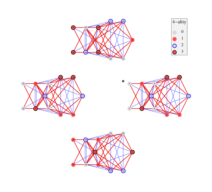
Figure 1: The left chiral graph of quantum symmetries ${\rm Oc}(\mathcal{E}_{4})$. Multiplication by the left chiral generator $100$ labeled 5 (resp. $001$ labeled 10) is encoded by oriented red edges (thick lines), in the direction of increasing (resp. decreasing) 4-ality. Multiplication by $010$ labeled 8 is encoded by unoriented blue egdes (thin lines).

We display in Fig. 1 the graph (with $48$ vertices) describing the multiplication by the chiral left generators. Multiplication by $100$ (resp. $001$) is encoded by oriented red edges (thick lines), in the direction of increasing (resp. decreasing) 4-ality, and multiplication by $010$ is encoded by unoriented blue edges (thin lines). The identity in $\mathcal{O}$ is marked with a star on the graph. The vertex representing the fundamental left generator of type $f$ is the neighbour of the identity along the corresponding edge (of type $f$) in the left chiral graph of quantum symmetry. The chiral adjoint operation (that interchanges matrices $O_{f^{L}}$ and ${O_{{\overline{f}}^{R}}}$) is given by the following table, where we list only the non trivial pairs that are interchanged by this operation:

$$\begin{array}[]{c|cccccccccccccccccc}\hline\cr&&\\ x&3&4&5&6&7&8&10&11&12&17&18&19&22&23&24&30&31&34\\ x^{{\dagger}}&13&14&33&37&38&21&45&25&26&32&39&40&44&27&28&47&48&41\\ &&\\ \hline\cr\end{array}$$

There are 12 self-adjoint generators ($x=x^{{\dagger}}$), ambichiral ones are 1, 2 and 9.

Adjacency matrices of $\boldsymbol{{\mathcal{E}}_{4}}$. We order vertices $x$ of the left quantum graph in such a way that connected components are separated in blocks. With this choice, the left chiral generator matrices take the following block diagonal form (see also [12]): $O_{100}^{L}={\rm diag}(G_{100},G_{100},G_{100},G_{100})$, $O_{010}^{L}={\rm diag}(G_{010},G_{010},G_{010},G_{010})$. $G_{100}$ is obtained from the decomposition of $O_{100}^{L}$ (or of $O_{100}^{R}$) in connected components, and $G_{010}$ from the decomposition of $O_{010}^{L}$ (or of $O_{010}^{R}$). For the $G_{f}$ matrices, we order the basis elements by increasing 4-ality

$$G_{100}=\left(\begin{array}[]{@{\,\,}c@{\,\,}c@{\,\,}c@{\,\,}c@{\,\,}c@{\,\,}c@{\,\,}c@{\,\,}c@{\,\,}c@{\,\,}c@{\,\,}c@{\,\,}c@{\,\,}}.&.&.&.&1&.&.&.&.&.&.&.\\ .&.&.&.&1&.&.&.&.&.&.&.\\ .&.&.&.&1&1&1&.&.&.&.&.\\ .&.&.&.&1&1&1&.&.&.&.&.\\ .&.&.&.&.&.&.&2&.&.&.&.\\ .&.&.&.&.&.&.&1&1&.&.&.\\ .&.&.&.&.&.&.&1&1&.&.&.\\ .&.&.&.&.&.&.&.&.&2&1&1\\ .&.&.&.&.&.&.&.&.&.&1&1\\ 1&1&1&1&.&.&.&.&.&.&.&.\\ .&.&1&1&.&.&.&.&.&.&.&.\\ .&.&1&1&.&.&.&.&.&.&.&.\end{array}\right),\qquad G_{010}=\left(\begin{array}[]{@{\,\,}c@{\,\,}c@{\,\,}c@{\,\,}c@{\,\,}c@{\,\,}c@{\,\,}c@{\,\,}c@{\,\,}c@{\,\,}c@{\,\,}c@{\,\,}c@{\,\,}}.&.&.&.&.&.&.&1&.&.&.&.\\ .&.&.&.&.&.&.&1&.&.&.&.\\ .&.&.&.&.&.&.&2&1&.&.&.\\ .&.&.&.&.&.&.&2&1&.&.&.\\ .&.&.&.&.&.&.&.&.&2&1&1\\ .&.&.&.&.&.&.&.&.&1&1&1\\ .&.&.&.&.&.&.&.&.&1&1&1\\ 1&1&2&2&.&.&.&.&.&.&.&.\\ .&.&1&1&.&.&.&.&.&.&.&.\\ .&.&.&.&2&1&1&.&.&.&.&.\\ .&.&.&.&1&1&1&.&.&.&.&.\\ .&.&.&.&1&1&1&.&.&.&.&.\end{array}\right).$$

It is now easy to determine the annular matrices $F_{n}$, the horizontal dimensions $d_{n}$, the total horizontal dimension $d_{H}$ and the dimension $d_{{\mathcal{B}}}$ of the quantum groupoïd ${\mathcal{B}}({\mathcal{E}}_{4})$. One can also calculate the quantum dimensions of simple objects of ${\mathcal{E}}_{4}$ and check the already obtained value for the quantum cardinality $|{\mathcal{E}}_{4}|$. Results are summarized in the table of Section 2.3.

Real-ambichiral partition functions of $\boldsymbol{{\mathcal{E}}_{4}}$ (i.e., $x=\overline{x}$, $x=x^{{\dagger}}$ and $x\in{\mathcal{J}}$). Here, such $x$’s coincide with ambichiral ones. Setting $U=004+101+121+400$, $V=000+012+040+210$, $W=U+V$ and $X=111$, we get

$$Z_{1}=4\overline{X}\;X+\overline{U}U+\overline{V}V\qquad\mbox{(the modular invariant partition function $\mathcal{Z}$)},$$

$$Z_{2}=4\overline{X}\;X+U\overline{V}+\overline{U}V,\qquad Z_{9}=2\overline{X}W+2\;\overline{W}X.$$

No exceptional module for ${\mathcal{E}}_{4}$. Since the permutation matrix $\mathfrak{C}$ commutes with $s$ and $t$, we may think of considering the new modular invariant matrix ${\mathcal{M}}^{\mathfrak{c}}=\mathfrak{C}\,{\mathcal{M}}$. However, in this particular case, ${\mathcal{M}}^{\mathfrak{c}}={\mathcal{M}}$, and we do not discover any new invariant in this way. Moreover the graph ${\mathcal{O}}$ of quantum symmetries contains only copies of the quantum graph ${\mathcal{E}}_{4}$. So we do not find any exceptional module in this case.

2.5 $\boldsymbol{{\rm Oc}({\mathcal{E}}_{6}({\rm SU}(4))}$

We consider the matrices ${\mathcal{K}}_{mn}$, keeping only those that are distinct, corresponding to each one of the possible norms $u$. For instance there are $30$ (distinct) matrices in norm 1 (i.e., $\#({\mathcal{K}}^{1})=30$), then $104$ in norm $2$ (i.e., $\#({\mathcal{K}}^{2})=104$), then $32,130,26,50,70,64,44,\ldots,2$ of them for the other possible norms. A first analysis gives immediately $30$ toric matrices in norm $1$, therefore all elements of ${\mathcal{K}}^{1}$, in particular ${\mathcal{K}}^{1}[1]=W_{00}={\mathcal{M}}$, then we find $36$ new ones in norm $2$ (many cases remaining unsettled at that stage), $4$ other in norm $3$ and $2$ in norm $12$ (but with multiplicity $5$), therefore a total of $72$ independent ones. A refined analysis of the norm $2$ case gives us $28$ more toric matrices, so that we have now reached the expected rank $r_{W}=100$. We are still missing $12=r_{O}-r_{W}$ others that should not be independent of those already found. $8$ $(=2\times 5-2)$ among them are immediately obtained from the fact that those coming from the norm $12$ analysis had multiplicity $5$. The last four are harder to find and are obtained after a deeper analysis of the norm $2$ case: they can be expressed as differences between a matrix belonging to the set ${\mathcal{K}}^{2}$ and a toric matrix previously determined in our analysis of the norm $3$ case (their matrix elements are nevertheless non-negative integers, of course). We then verify that all equations for the $46$ possible norms can be satisfied with the obtained $112$ toric matrices, and that the equation of modular splitting, itself, holds.

The next step is to solve the intertwining equations that determine the $6$ matrices expressing the generators of ${\mathcal{O}}$ using the methods described previously. Here again there are several free parameters still remaining after resolution of these equations, but they are subsequently determined by using non negativity and integrality of coefficients, commutation properties of generators, and imposing that the ${\rm SU}(4)$ polynomials $y_{7}$, $y_{8}$, $y_{9}$ should vanish.

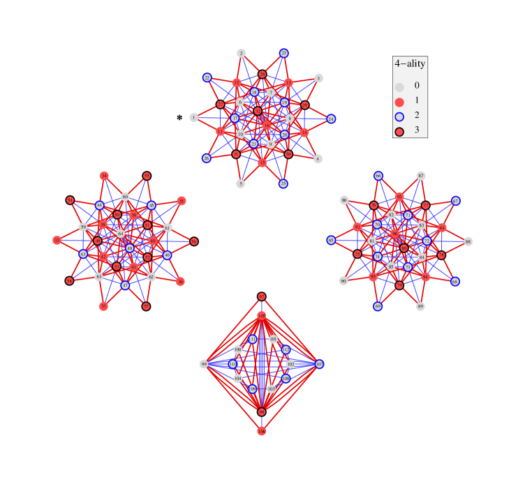
Figure 2: The left chiral graph of quantum symmetries ${\rm Oc}(\mathcal{E}_{6})$. Multiplication by the left chiral generator $100$ labeled 11 (resp. $001$ labeled 27) is encoded by oriented red edges (thick lines), in the direction of increasing (resp. decreasing) 4-ality. Multiplication by $010$ labeled 17 is encoded by unoriented blue edges (thin lines).

We display in Fig. 2 the graph (with $112$ vertices) describing the multiplication by the chiral left generators, where we adopt the same conventions as for the $\mathcal{E}_{4}$ case. The graph of quantum symmetries contains 4 connected components, the quantum graph $\mathcal{E}_{6}$ appears 3 times, and a module, that we call $\mathcal{E}_{6}^{\mathfrak{c}}$, appears once. The chiral adjoint operation (that interchanges matrices $O_{f^{L}}$ and ${O_{{\overline{f}}^{R}}}$) is given by the following table, where we list only the non trivial pairs that are interchanged by this operation,

$$\begin{array}[]{c|cccccccccccccccccccccccc}\hline\cr&&\\ x&6&7&8&9&10&11&12&13&14&15&16&17&18&19&20&21&27&28&29&30\\ x^{{\dagger}}&86&87&88&89&90&58&54&55&56&57&97&65&66&67&68&69&33&34&35&36\\ &&\\ x&31&32&38&39&40&41&42&48&49&50&51&52&53&64&80&96&&&&\\ x^{{\dagger}}&37&106&76&77&78&79&75&107&91&92&93&94&95&99&105&98&&&&\\ &&\\ \hline\cr\end{array}$$

There are 40 self-adjoint vertices ($x=x^{{\dagger}}$), ambichiral ones are (1, 2, 3, 4, 5, 22, 23, 24, 25, 26).

Adjacency matrices of $\boldsymbol{{\mathcal{E}}_{6}}$ and $\boldsymbol{{\mathcal{E}}_{6}^{\mathfrak{c}}}$. We order vertices $x$ of the left quantum graph in such a way that connected components are separated in blocks. The left chiral generator matrices take the following block diagonal form: $O_{100}^{L}={\rm diag}(G_{100},G_{100},G_{100},{G_{100}}^{\mathfrak{c}})$, $O_{010}^{L}={\rm diag}(G_{010},G_{010},G_{010},{G_{010}}^{\mathfrak{c}})$. Matrices $G_{100}$ and ${G_{100}}^{\mathfrak{c}}$ are obtained from the decomposition of $O_{100}^{L}$ (or of $O_{100}^{R}$) in connected components, $G_{010}$ and ${G_{010}}^{\mathfrak{c}}$ from the decomposition of $O_{010}^{L}$ (or of $O_{010}^{R}$). For the $G_{f}$ matrices, we order the basis elements by increasing 4-ality.

For the ${\mathcal{E}}_{6}$ graph we obtain:

$$G_{100}=\left(\begin{array}[]{@{\,\,}c@{\,\,}c@{\,\,}c@{\,\,}c@{\,\,}c@{\,\,}c@{\,\,}c@{\,\,}c@{\,\,}c@{\,\,}c@{\,\,}c@{\,\,}c@{\,\,}c@{\,\,}c@{\,\,}c@{\,\,}c@{\,\,}c@{\,\,}c@{\,\,}c@{\,\,}c@{\,\,}c@{\,\,}c@{\,\,}c@{\,\,}c@{\,\,}c@{\,\,}c@{\,\,}c@{\,\,}c@{\,\,}c@{\,\,}c@{\,\,}c@{\,\,}c@{\,\,}}.&.&.&.&.&.&.&.&.&.&1&.&.&.&.&.&.&.&.&.&.&.&.&.&.&.&.&.&.&.&.&.\\ .&.&.&.&.&.&.&.&.&.&.&1&.&.&.&.&.&.&.&.&.&.&.&.&.&.&.&.&.&.&.&.\\ .&.&.&.&.&.&.&.&.&.&.&.&1&.&.&.&.&.&.&.&.&.&.&.&.&.&.&.&.&.&.&.\\ .&.&.&.&.&.&.&.&.&.&.&.&.&1&.&.&.&.&.&.&.&.&.&.&.&.&.&.&.&.&.&.\\ .&.&.&.&.&.&.&.&.&.&.&.&.&.&1&.&.&.&.&.&.&.&.&.&.&.&.&.&.&.&.&.\\ .&.&.&.&.&.&.&.&.&.&1&1&.&.&.&1&.&.&.&.&.&.&.&.&.&.&.&.&.&.&.&.\\ .&.&.&.&.&.&.&.&.&.&.&1&1&.&.&1&.&.&.&.&.&.&.&.&.&.&.&.&.&.&.&.\\ .&.&.&.&.&.&.&.&.&.&.&.&1&1&.&1&.&.&.&.&.&.&.&.&.&.&.&.&.&.&.&.\\ .&.&.&.&.&.&.&.&.&.&.&.&.&1&1&1&.&.&.&.&.&.&.&.&.&.&.&.&.&.&.&.\\ .&.&.&.&.&.&.&.&.&.&1&.&.&.&1&1&.&.&.&.&.&.&.&.&.&.&.&.&.&.&.&.\\ .&.&.&.&.&.&.&.&.&.&.&.&.&.&.&.&1&.&.&.&1&.&.&.&.&1&.&.&.&.&.&.\\ .&.&.&.&.&.&.&.&.&.&.&.&.&.&.&.&1&1&.&.&.&1&.&.&.&.&.&.&.&.&.&.\\ .&.&.&.&.&.&.&.&.&.&.&.&.&.&.&.&.&1&1&.&.&.&1&.&.&.&.&.&.&.&.&.\\ .&.&.&.&.&.&.&.&.&.&.&.&.&.&.&.&.&.&1&1&.&.&.&1&.&.&.&.&.&.&.&.\\ .&.&.&.&.&.&.&.&.&.&.&.&.&.&.&.&.&.&.&1&1&.&.&.&1&.&.&.&.&.&.&.\\ .&.&.&.&.&.&.&.&.&.&.&.&.&.&.&.&1&1&1&1&1&.&.&.&.&.&.&.&.&.&.&.\\ .&.&.&.&.&.&.&.&.&.&.&.&.&.&.&.&.&.&.&.&.&.&.&.&.&.&1&.&.&.&1&1\\ .&.&.&.&.&.&.&.&.&.&.&.&.&.&.&.&.&.&.&.&.&.&.&.&.&.&1&1&.&.&.&1\\ .&.&.&.&.&.&.&.&.&.&.&.&.&.&.&.&.&.&.&.&.&.&.&.&.&.&.&1&1&.&.&1\\ .&.&.&.&.&.&.&.&.&.&.&.&.&.&.&.&.&.&.&.&.&.&.&.&.&.&.&.&1&1&.&1\\ .&.&.&.&.&.&.&.&.&.&.&.&.&.&.&.&.&.&.&.&.&.&.&.&.&.&.&.&.&1&1&1\\ .&.&.&.&.&.&.&.&.&.&.&.&.&.&.&.&.&.&.&.&.&.&.&.&.&.&1&.&.&.&.&.\\ .&.&.&.&.&.&.&.&.&.&.&.&.&.&.&.&.&.&.&.&.&.&.&.&.&.&.&1&.&.&.&.\\ .&.&.&.&.&.&.&.&.&.&.&.&.&.&.&.&.&.&.&.&.&.&.&.&.&.&.&.&1&.&.&.\\ .&.&.&.&.&.&.&.&.&.&.&.&.&.&.&.&.&.&.&.&.&.&.&.&.&.&.&.&.&1&.&.\\ .&.&.&.&.&.&.&.&.&.&.&.&.&.&.&.&.&.&.&.&.&.&.&.&.&.&.&.&.&.&1&.\\ 1&.&.&.&.&1&.&.&.&1&.&.&.&.&.&.&.&.&.&.&.&.&.&.&.&.&.&.&.&.&.&.\\ .&1&.&.&.&1&1&.&.&.&.&.&.&.&.&.&.&.&.&.&.&.&.&.&.&.&.&.&.&.&.&.\\ .&.&1&.&.&.&1&1&.&.&.&.&.&.&.&.&.&.&.&.&.&.&.&.&.&.&.&.&.&.&.&.\\ .&.&.&1&.&.&.&1&1&.&.&.&.&.&.&.&.&.&.&.&.&.&.&.&.&.&.&.&.&.&.&.\\ .&.&.&.&1&.&.&.&1&1&.&.&.&.&.&.&.&.&.&.&.&.&.&.&.&.&.&.&.&.&.&.\\ .&.&.&.&.&1&1&1&1&1&.&.&.&.&.&.&.&.&.&.&.&.&.&.&.&.&.&.&.&.&.&.\end{array}\right)$$,

$$G_{010}=\left(\begin{array}[]{@{\,\,}c@{\,\,}c@{\,\,}c@{\,\,}c@{\,\,}c@{\,\,}c@{\,\,}c@{\,\,}c@{\,\,}c@{\,\,}c@{\,\,}c@{\,\,}c@{\,\,}c@{\,\,}c@{\,\,}c@{\,\,}c@{\,\,}c@{\,\,}c@{\,\,}c@{\,\,}c@{\,\,}c@{\,\,}c@{\,\,}c@{\,\,}c@{\,\,}c@{\,\,}c@{\,\,}c@{\,\,}c@{\,\,}c@{\,\,}c@{\,\,}c@{\,\,}c@{\,\,}}.&.&.&.&.&.&.&.&.&.&.&.&.&.&.&.&1&.&.&.&.&.&.&.&.&.&.&.&.&.&.&.\\ .&.&.&.&.&.&.&.&.&.&.&.&.&.&.&.&.&1&.&.&.&.&.&.&.&.&.&.&.&.&.&.\\ .&.&.&.&.&.&.&.&.&.&.&.&.&.&.&.&.&.&1&.&.&.&.&.&.&.&.&.&.&.&.&.\\ .&.&.&.&.&.&.&.&.&.&.&.&.&.&.&.&.&.&.&1&.&.&.&.&.&.&.&.&.&.&.&.\\ .&.&.&.&.&.&.&.&.&.&.&.&.&.&.&.&.&.&.&.&1&.&.&.&.&.&.&.&.&.&.&.\\ .&.&.&.&.&.&.&.&.&.&.&.&.&.&.&.&1&1&1&.&1&1&.&.&.&.&.&.&.&.&.&.\\ .&.&.&.&.&.&.&.&.&.&.&.&.&.&.&.&1&1&1&1&.&.&1&.&.&.&.&.&.&.&.&.\\ .&.&.&.&.&.&.&.&.&.&.&.&.&.&.&.&.&1&1&1&1&.&.&1&.&.&.&.&.&.&.&.\\ .&.&.&.&.&.&.&.&.&.&.&.&.&.&.&.&1&.&1&1&1&.&.&.&1&.&.&.&.&.&.&.\\ .&.&.&.&.&.&.&.&.&.&.&.&.&.&.&.&1&1&.&1&1&.&.&.&.&1&.&.&.&.&.&.\\ .&.&.&.&.&.&.&.&.&.&.&.&.&.&.&.&.&.&.&.&.&.&.&.&.&.&1&.&.&.&1&1\\ .&.&.&.&.&.&.&.&.&.&.&.&.&.&.&.&.&.&.&.&.&.&.&.&.&.&1&1&.&.&.&1\\ .&.&.&.&.&.&.&.&.&.&.&.&.&.&.&.&.&.&.&.&.&.&.&.&.&.&.&1&1&.&.&1\\ .&.&.&.&.&.&.&.&.&.&.&.&.&.&.&.&.&.&.&.&.&.&.&.&.&.&.&.&1&1&.&1\\ .&.&.&.&.&.&.&.&.&.&.&.&.&.&.&.&.&.&.&.&.&.&.&.&.&.&.&.&.&1&1&1\\ .&.&.&.&.&.&.&.&.&.&.&.&.&.&.&.&.&.&.&.&.&.&.&.&.&.&1&1&1&1&1&2\\ 1&.&.&.&.&1&1&.&1&1&.&.&.&.&.&.&.&.&.&.&.&.&.&.&.&.&.&.&.&.&.&.\\ .&1&.&.&.&1&1&1&.&1&.&.&.&.&.&.&.&.&.&.&.&.&.&.&.&.&.&.&.&.&.&.\\ .&.&1&.&.&1&1&1&1&.&.&.&.&.&.&.&.&.&.&.&.&.&.&.&.&.&.&.&.&.&.&.\\ .&.&.&1&.&.&1&1&1&1&.&.&.&.&.&.&.&.&.&.&.&.&.&.&.&.&.&.&.&.&.&.\\ .&.&.&.&1&1&.&1&1&1&.&.&.&.&.&.&.&.&.&.&.&.&.&.&.&.&.&.&.&.&.&.\\ .&.&.&.&.&1&.&.&.&.&.&.&.&.&.&.&.&.&.&.&.&.&.&.&.&.&.&.&.&.&.&.\\ .&.&.&.&.&.&1&.&.&.&.&.&.&.&.&.&.&.&.&.&.&.&.&.&.&.&.&.&.&.&.&.\\ .&.&.&.&.&.&.&1&.&.&.&.&.&.&.&.&.&.&.&.&.&.&.&.&.&.&.&.&.&.&.&.\\ .&.&.&.&.&.&.&.&1&.&.&.&.&.&.&.&.&.&.&.&.&.&.&.&.&.&.&.&.&.&.&.\\ .&.&.&.&.&.&.&.&.&1&.&.&.&.&.&.&.&.&.&.&.&.&.&.&.&.&.&.&.&.&.&.\\ .&.&.&.&.&.&.&.&.&.&1&1&.&.&.&1&.&.&.&.&.&.&.&.&.&.&.&.&.&.&.&.\\ .&.&.&.&.&.&.&.&.&.&.&1&1&.&.&1&.&.&.&.&.&.&.&.&.&.&.&.&.&.&.&.\\ .&.&.&.&.&.&.&.&.&.&.&.&1&1&.&1&.&.&.&.&.&.&.&.&.&.&.&.&.&.&.&.\\ .&.&.&.&.&.&.&.&.&.&.&.&.&1&1&1&.&.&.&.&.&.&.&.&.&.&.&.&.&.&.&.\\ .&.&.&.&.&.&.&.&.&.&1&.&.&.&1&1&.&.&.&.&.&.&.&.&.&.&.&.&.&.&.&.\\ .&.&.&.&.&.&.&.&.&.&1&1&1&1&1&2&.&.&.&.&.&.&.&.&.&.&.&.&.&.&.&.\end{array}\right)$$

and for the ${\mathcal{E}}_{6}^{\mathfrak{c}}$ graph:

$$G_{100}^{\mathfrak{c}}=\left(\begin{array}[]{@{\,\,}c@{\,\,}c@{\,\,}c@{\,\,}c@{\,\,}c@{\,\,}c@{\,\,}c@{\,\,}c@{\,\,}c@{\,\,}c@{\,\,}c@{\,\,}c@{\,\,}c@{\,\,}c@{\,\,}c@{\,\,}c@{\,\,}}.&.&1&.&.&.&.&.&.&.&.&.&.&.&.&.\\ .&.&2&1&1&1&1&1&.&.&.&.&.&.&.&.\\ .&.&.&.&.&.&.&.&2&1&.&.&.&.&.&.\\ .&.&.&.&.&.&.&.&1&.&.&.&.&.&.&.\\ .&.&.&.&.&.&.&.&1&.&.&.&.&.&.&.\\ .&.&.&.&.&.&.&.&1&.&.&.&.&.&.&.\\ .&.&.&.&.&.&.&.&1&.&.&.&.&.&.&.\\ .&.&.&.&.&.&.&.&1&.&.&.&.&.&.&.\\ .&.&.&.&.&.&.&.&.&.&2&1&1&1&1&1\\ .&.&.&.&.&.&.&.&.&.&1&.&.&.&.&.\\ 1&2&.&.&.&.&.&.&.&.&.&.&.&.&.&.\\ .&1&.&.&.&.&.&.&.&.&.&.&.&.&.&.\\ .&1&.&.&.&.&.&.&.&.&.&.&.&.&.&.\\ .&1&.&.&.&.&.&.&.&.&.&.&.&.&.&.\\ .&1&.&.&.&.&.&.&.&.&.&.&.&.&.&.\\ .&1&.&.&.&.&.&.&.&.&.&.&.&.&.&.\end{array}\right),\qquad G_{010}^{\mathfrak{c}}=\left(\begin{array}[]{@{\,\,}c@{\,\,}c@{\,\,}c@{\,\,}c@{\,\,}c@{\,\,}c@{\,\,}c@{\,\,}c@{\,\,}c@{\,\,}c@{\,\,}c@{\,\,}c@{\,\,}c@{\,\,}c@{\,\,}c@{\,\,}c@{\,\,}}.&.&.&.&.&.&.&.&1&.&.&.&.&.&.&.\\ .&.&.&.&.&.&.&.&4&1&.&.&.&.&.&.\\ .&.&.&.&.&.&.&.&.&.&2&1&1&1&1&1\\ .&.&.&.&.&.&.&.&.&.&1&.&.&1&1&.\\ .&.&.&.&.&.&.&.&.&.&1&.&.&.&1&1\\ .&.&.&.&.&.&.&.&.&.&1&1&.&.&.&1\\ .&.&.&.&.&.&.&.&.&.&1&1&1&.&.&.\\ .&.&.&.&.&.&.&.&.&.&1&.&1&1&.&.\\ 1&4&.&.&.&.&.&.&.&.&.&.&.&.&.&.\\ .&1&.&.&.&.&.&.&.&.&.&.&.&.&.&.\\ .&.&2&1&1&1&1&1&.&.&.&.&.&.&.&.\\ .&.&1&.&.&1&1&.&.&.&.&.&.&.&.&.\\ .&.&1&.&.&.&1&1&.&.&.&.&.&.&.&.\\ .&.&1&1&.&.&.&1&.&.&.&.&.&.&.&.\\ .&.&1&1&1&.&.&.&.&.&.&.&.&.&.&.\\ .&.&1&.&1&1&.&.&.&.&.&.&.&.&.&.\end{array}\right)$$.

It is now easy to determine the annular matrices $F_{n}$, the horizontal dimensions $d_{n}$, the total horizontal dimension $d_{H}$ and the dimension $d_{{\mathcal{B}}}$ of the quantum groupoïd ${\mathcal{B}}({\mathcal{E}}_{6})$. One can also calculate the quantum dimensions of simple objects of ${\mathcal{E}}_{6}$ and check the already obtained value for the quantum cardinality $|{\mathcal{E}}_{6}|$. Results are summarized in the table of Section 2.3.

Real-ambichiral partition functions of $\boldsymbol{{\mathcal{E}}_{6}}$ (i.e., $x=\overline{x}$, $x=x^{{\dagger}}$ and $x\in{\mathcal{J}}$). Here, there are only two such $x$’s, but $10$ ambichiral vertices. Setting

$$U_{1}=000+060+202+222,\qquad U_{2}=006+022+220+600,$$

$$V_{1}=042+200+212,\qquad V_{2}=012+230+303,\qquad V_{3}=030+103+321,$$

$$V_{4}=004+121+420,\qquad V_{5}=030+123+301,\qquad V_{6}=024+121+400,$$

$$V_{7}=032+210+303,\qquad V_{8}=002+212+240$$

we obtain

$$Z_{1}=\overline{U_{1}}U_{1}+\overline{U_{2}}U_{2}+\overline{V_{1}}V_{1}+\overline{V_{2}}V_{2}+\overline{V_{3}}V_{3}+\overline{V_{4}}V_{4}+\overline{V_{5}}V_{5}+\overline{V_{6}}V_{6}+\overline{V_{7}}V_{7}+\overline{V_{8}}V_{8},$$

$$Z_{24}=\overline{U_{1}}U_{2}+\overline{U_{2}}U_{1}+\overline{V_{1}}V_{4}+\overline{V_{4}}V_{1}+\overline{V_{2}}V_{5}+\overline{V_{5}}V_{2}+\overline{V_{3}}V_{7}+\overline{V_{7}}V_{3}+\overline{V_{6}}V_{8}+\overline{V_{8}}V_{6}$$

and in particular we recognize the modular invariant $\mathcal{Z}=Z_{1}$.

An exceptional module for $\boldsymbol{{\mathcal{E}}_{6}}$. Since the permutation matrix $\mathfrak{C}$ commutes with $s$ and $t$, we may think of considering the new modular invariant matrix ${\mathcal{M}}^{\mathfrak{c}}=\mathfrak{C}\,{\mathcal{M}}$. Here, ${\mathcal{M}}^{\mathfrak{c}}\neq{\mathcal{M}}$ and we find a new invariant. Using the above notations, the corresponding partition function $\mathcal{Z}^{\mathfrak{c}}=\sum_{\lambda}\chi_{\lambda}\,{\mathcal{M}}^{\mathfrak{c}}_{\lambda\mu}\,\bar{\chi}_{\mu}$, which is of type-II, (the modular invariant is not a sum of blocks) reads:

$${Z_{1}}^{\mathfrak{c}}=\overline{U_{1}}U_{1}+\overline{U_{2}}U_{2}+\overline{V_{1}}V_{8}+\overline{V_{2}}V_{7}+\overline{V_{3}}V_{5}+\overline{V_{4}}V_{6}+\overline{V_{5}}V_{3}+\overline{V_{6}}V_{4}+\overline{V_{7}}V_{2}+\overline{V_{8}}V_{1}.$$

Its own quantum graph, denoted ${{\mathcal{E}}_{6}}^{\mathfrak{c}}$ appears as a module in the graph of quantum symmetries of ${\mathcal{O}}({\mathcal{E}}_{6})$. It has $16={\rm Tr}({\mathcal{M}}^{\mathfrak{c}})=r_{E}/2$ vertices. One can then study it directly, i.e., determine its own annular matrices, its own algebra of quantum symmetries etc. Since the quantum graph ${{\mathcal{E}}_{6}}^{\mathfrak{c}}$ is known from the very beginning (its adjacency matrices ${G_{f}}^{\mathfrak{c}}$, given previously, are obtained from the connected components of ${\mathcal{O}}({\mathcal{E}}_{6})$ which are not of type ${\mathcal{E}}_{6}$), the analysis is much easier than for ${\mathcal{E}}_{6}$. The ${\mathcal{A}}$ module structure of ${{\mathcal{E}}_{6}}$ and ${{\mathcal{E}}_{6}}^{\mathfrak{c}}$ differ (not the same annular matrices, of course). One finds $d_{H}=\sum_{n}\,d_{n}=11456=2^{6}179^{1}$ and $d_{\mathcal{B}}=\sum_{n}\,{d_{n}}^{2}=2152960=2^{9}5^{1}29^{2}$. Notice that ${{\mathcal{E}}_{6}}^{\mathfrak{c}}$ has no self-fusion. As expected, ${\mathcal{O}}({\mathcal{E}}_{6})$ and ${\mathcal{O}}({{\mathcal{E}}_{6}}^{\mathfrak{c}})$ are isomorphic algebras, but their realizations, in terms of the graph algebra of ${\mathcal{E}}_{6}$, are different.

2.6 $\boldsymbol{{\rm Oc}({\mathcal{E}}_{8}({\rm SU}(4))}$

We consider the matrices ${\mathcal{K}}_{mn}$, keeping only those that are distinct, corresponding to each one of the possible norms $u$. For instance there are $63$ (distinct) matrices in norm 1 (i.e., $\#({\mathcal{K}}^{1})=63$), then $48$ in norm $2$ (i.e., $\#({\mathcal{K}}^{2})=48$), then $38,71,25,36,26,60,16,18,32,38,30,36,9,\ldots$ of them for the other possible norms. A first analysis gives immediately $63$ toric matrices in norm $1$, therefore all elements of ${\mathcal{K}}^{1}$, in particular ${\mathcal{K}}^{1}[1]=W_{00}={\mathcal{M}}$ , then we find $48$ new ones in norm $2$ (among them, $23$ appear with multiplicity $2$), $8$ others in norm $3$ (all of them with multiplicity $2$), $16$ in norm $4$ (among them, $12$ with multiplicity $2$, and $8$ entries remain unsettled cases at that stage), $3$ in norm $5$ (among them, $3$ with multiplicity $2$), $4$ in norm $6$ (no multiplicities), $1$ in norm $7$ (with multiplicity $2$), nothing in norms 8, 9, 10, 11, 12, 14, but $1$ in norm $15$ (with multiplicity $2$) so that we reach a total of $63+48+8+16+3+4+1+1=144=r_{W}$, the expected rank. After having checked that the $8$ unsettled cases remaining in length $4$ can be reexpressed in terms of the others, we take into account the already determined multiplicities and see that $23+8+12+3+1+1=48$, so that we can easily complete the family since $144+48=192=r_{O}$. We then verify that all equations for the $142$ possible norms can be satisfied with the obtained $192$ toric matrices, and that the equation of modular splitting, itself, holds.

This case ${\mathcal{E}}_{8}$ involves huge computations, compared with the previous cases (the tensor ${\mathcal{K}}$ contains $40869849$ non-zero entries), but, fortunately, the resolution of the equation of modular splitting is somehow easier than in the ${\mathcal{E}}_{6}$ case (in particular, the determination of the $r_{O}-r_{W}$ matrices needed to complete the family).

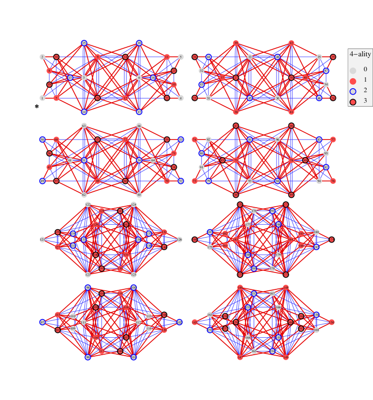
Figure 3: The left chiral graph of quantum symmetries ${\rm Oc}(\mathcal{E}_{8})$. Multiplication by the left chiral generator $100$ labeled 7 (resp. $001$ labeled 19) is encoded by oriented red edges (thick lines), in the direction of increasing (resp. decreasing) 4-ality. Multiplication by $010$ labeled 13 is encoded by unoriented blue edges (thin lines).

The next step is to solve the intertwining equations that determine the $6$ matrices expressing the fundamental generators of ${\mathcal{O}}$. Eliminating arbitrary coefficients in those matrices is actually a rather hard and tedious task involving simultaneously all the constraints and methods described previously (integrality, positivity, intertwining equations, commutation with complex conjugates and with chiral partners, polynomial identities in degrees 9, 10, 11). At the very end we obtain, up to reordering of the $192$ vertices, a single solution $O_{{010}^{L,R}}$ for the matrices of the left and right symmetric generators, a single solution for the left generator $O_{{100}^{L}}$ (that we block diagonalize in the form given below) but several solutions for the corresponding right generator $O_{{100}^{R}}$. However, the non unicity of the solutions for the pair of fundamental generators $(O_{{100}^{L}},O_{{100}^{R}})$ reflects the existence of graph automorphisms (see our discussion in Section 2.2); for instance one of them exchanges vertices $17$ with $18$, or $122$ with $123$ (see Fig. 3). For each of these choices (for definiteness we select one of these equivalent solutions and just call it ${O}_{{100}^{R}}$) one can find several distinct permutation matrices $Q$, with $Q=\tilde{Q}=Q^{-1}$ such that ${O}_{{100}^{R}}=Q\,{O}_{{001}^{L}}\,Q^{-1}$. We then restrict the possible choices for this matrix in the manner discussed at page 2.2. The permutation associated with the chiral adjoint matrix $Q$ that interchanges matrices $O_{f^{L}}$ and ${O_{{\overline{f}}^{R}}}$, up to graph isomorphisms, is given below (as before, we list only the non trivial pairs that are interchanged by this operation).

$$\begin{array}[]{c|cccccccccccccccccccc}\hline\cr&&\\ x&3&6&7&8&9&10&11&12&13&14&15&16&17&18&19&20&21&22&23&24\\ x^{{\dagger}}&121&126&25&26&174&28&29&169&97&49&50&102&52&53&73&74&150&76&77&145\\[2.84526pt] x&27&30&33&36&37&38&39&40&41&42&43&44&45&46&47&48&51&54&57&60\\ x^{{\dagger}}&127&132&180&175&103&55&56&108&58&59&79&80&156&82&83&151&135&136&184&183\\[2.84526pt] x&61&64&67&68&69&70&71&72&75&78&81&84&85&88&93&96&98&99&100&101\\ x^{{\dagger}}&111&112&86&87&160&89&90&159&139&144&192&187&115&120&168&163&133&134&138&137\\[2.84526pt] x&104&105&106&107&116&117&118&119&128&129&130&131&140&141&142&143&152&153&154&155\\ x^{{\dagger}}&185&186&181&182&162&161&158&157&173&172&170&171&148&149&147&146&189&188&191&190\\[2.84526pt] \hline\cr\end{array}$$

There are $32$ self-adjoint vertices ($x=x^{{\dagger}}$), ambichiral ones are 1, 2, 4, 5 (the toric matrices associated with vertices $4$ and $5$ are actually equal).

Adjacency matrices of $\boldsymbol{{\mathcal{E}}_{8}}$. We order vertices $x$ of the left quantum graph in such a way that connected components are separated in blocks. The left chiral generator matrices take the following block diagonal form: $O_{100}^{L}={\rm diag}(G_{100},G_{100},G_{100},G_{100},{G_{100}}^{\mathfrak{c}},{G_{100}}^{\mathfrak{c}},{G_{100}}^{\mathfrak{c}},{G_{100}}^{\mathfrak{c}})$, $O_{010}^{L}={\rm diag}(G_{010},G_{010},G_{010},G_{010},{G_{010}}^{\mathfrak{c}},{G_{010}}^{\mathfrak{c}},{G_{010}}^{\mathfrak{c}},{G_{010}}^{\mathfrak{c}})$. Matrices $G_{100}$ and ${G_{100}}^{\mathfrak{c}}$ are obtained from the decomposition of $O_{100}^{L}$ (or of $O_{100}^{R}$) in connected components, $G_{010}$ and ${G_{010}}^{\mathfrak{c}}$ from the decomposition of $O_{010}^{L}$ (or of $O_{010}^{R}$). For the $G_{f}$ matrices, we order the basis elements by increasing 4-ality,

$$G_{100}=\left(\begin{array}[]{@{\,\,}c@{\,\,}c@{\,\,}c@{\,\,}c@{\,\,}c@{\,\,}c@{\,\,}c@{\,\,}c@{\,\,}c@{\,\,}c@{\,\,}c@{\,\,}c@{\,\,}c@{\,\,}c@{\,\,}c@{\,\,}c@{\,\,}c@{\,\,}c@{\,\,}c@{\,\,}c@{\,\,}c@{\,\,}c@{\,\,}c@{\,\,}c@{\,\,}}.&.&.&.&.&.&1&.&.&.&.&.&.&.&.&.&.&.&.&.&.&.&.&.\\ .&.&.&.&.&.&.&1&.&.&.&.&.&.&.&.&.&.&.&.&.&.&.&.\\ .&.&.&.&.&.&1&1&2&.&.&1&.&.&.&.&.&.&.&.&.&.&.&.\\ .&.&.&.&.&.&.&.&.&1&.&.&.&.&.&.&.&.&.&.&.&.&.&.\\ .&.&.&.&.&.&.&.&.&.&1&.&.&.&.&.&.&.&.&.&.&.&.&.\\ .&.&.&.&.&.&.&.&1&1&1&2&.&.&.&.&.&.&.&.&.&.&.&.\\ .&.&.&.&.&.&.&.&.&.&.&.&1&1&.&.&.&.&.&.&.&.&.&.\\ .&.&.&.&.&.&.&.&.&.&.&.&1&.&1&.&.&.&.&.&.&.&.&.\\ .&.&.&.&.&.&.&.&.&.&.&.&1&1&1&.&1&1&.&.&.&.&.&.\\ .&.&.&.&.&.&.&.&.&.&.&.&.&.&.&1&1&.&.&.&.&.&.&.\\ .&.&.&.&.&.&.&.&.&.&.&.&.&.&.&1&.&1&.&.&.&.&.&.\\ .&.&.&.&.&.&.&.&.&.&.&.&.&1&1&1&1&1&.&.&.&.&.&.\\ .&.&.&.&.&.&.&.&.&.&.&.&.&.&.&.&.&.&1&1&1&.&.&.\\ .&.&.&.&.&.&.&.&.&.&.&.&.&.&.&.&.&.&.&1&1&.&.&1\\ .&.&.&.&.&.&.&.&.&.&.&.&.&.&.&.&.&.&1&.&1&.&.&1\\ .&.&.&.&.&.&.&.&.&.&.&.&.&.&.&.&.&.&.&.&.&1&1&1\\ .&.&.&.&.&.&.&.&.&.&.&.&.&.&.&.&.&.&.&.&1&.&1&1\\ .&.&.&.&.&.&.&.&.&.&.&.&.&.&.&.&.&.&.&.&1&1&.&1\\ 1&.&1&.&.&.&.&.&.&.&.&.&.&.&.&.&.&.&.&.&.&.&.&.\\ .&1&1&.&.&.&.&.&.&.&.&.&.&.&.&.&.&.&.&.&.&.&.&.\\ .&.&2&.&.&1&.&.&.&.&.&.&.&.&.&.&.&.&.&.&.&.&.&.\\ .&.&.&1&.&1&.&.&.&.&.&.&.&.&.&.&.&.&.&.&.&.&.&.\\ .&.&.&.&1&1&.&.&.&.&.&.&.&.&.&.&.&.&.&.&.&.&.&.\\ .&.&1&.&.&2&.&.&.&.&.&.&.&.&.&.&.&.&.&.&.&.&.&.\end{array}\right), G_{010}=\left(\begin{array}[]{@{\,\,}c@{\,\,}c@{\,\,}c@{\,\,}c@{\,\,}c@{\,\,}c@{\,\,}c@{\,\,}c@{\,\,}c@{\,\,}c@{\,\,}c@{\,\,}c@{\,\,}c@{\,\,}c@{\,\,}c@{\,\,}c@{\,\,}c@{\,\,}c@{\,\,}c@{\,\,}c@{\,\,}c@{\,\,}c@{\,\,}c@{\,\,}c@{\,\,}}.&.&.&.&.&.&.&.&.&.&.&.&1&.&.&.&.&.&.&.&.&.&.&.\\ .&.&.&.&.&.&.&.&.&.&.&.&1&.&.&.&.&.&.&.&.&.&.&.\\ .&.&.&.&.&.&.&.&.&.&.&.&2&2&2&.&1&1&.&.&.&.&.&.\\ .&.&.&.&.&.&.&.&.&.&.&.&.&.&.&1&.&.&.&.&.&.&.&.\\ .&.&.&.&.&.&.&.&.&.&.&.&.&.&.&1&.&.&.&.&.&.&.&.\\ .&.&.&.&.&.&.&.&.&.&.&.&.&1&1&2&2&2&.&.&.&.&.&.\\ .&.&.&.&.&.&.&.&.&.&.&.&.&.&.&.&.&.&1&1&1&.&.&.\\ .&.&.&.&.&.&.&.&.&.&.&.&.&.&.&.&.&.&1&1&1&.&.&.\\ .&.&.&.&.&.&.&.&.&.&.&.&.&.&.&.&.&.&1&1&2&.&.&2\\ .&.&.&.&.&.&.&.&.&.&.&.&.&.&.&.&.&.&.&.&.&1&1&1\\ .&.&.&.&.&.&.&.&.&.&.&.&.&.&.&.&.&.&.&.&.&1&1&1\\ .&.&.&.&.&.&.&.&.&.&.&.&.&.&.&.&.&.&.&.&2&1&1&2\\ 1&1&2&.&.&.&.&.&.&.&.&.&.&.&.&.&.&.&.&.&.&.&.&.\\ .&.&2&.&.&1&.&.&.&.&.&.&.&.&.&.&.&.&.&.&.&.&.&.\\ .&.&2&.&.&1&.&.&.&.&.&.&.&.&.&.&.&.&.&.&.&.&.&.\\ .&.&.&1&1&2&.&.&.&.&.&.&.&.&.&.&.&.&.&.&.&.&.&.\\ .&.&1&.&.&2&.&.&.&.&.&.&.&.&.&.&.&.&.&.&.&.&.&.\\ .&.&1&.&.&2&.&.&.&.&.&.&.&.&.&.&.&.&.&.&.&.&.&.\\ .&.&.&.&.&.&1&1&1&.&.&.&.&.&.&.&.&.&.&.&.&.&.&.\\ .&.&.&.&.&.&1&1&1&.&.&.&.&.&.&.&.&.&.&.&.&.&.&.\\ .&.&.&.&.&.&1&1&2&.&.&2&.&.&.&.&.&.&.&.&.&.&.&.\\ .&.&.&.&.&.&.&.&.&1&1&1&.&.&.&.&.&.&.&.&.&.&.&.\\ .&.&.&.&.&.&.&.&.&1&1&1&.&.&.&.&.&.&.&.&.&.&.&.\\ .&.&.&.&.&.&.&.&2&1&1&2&.&.&.&.&.&.&.&.&.&.&.&.\end{array}\right)$$

and for the ${\mathcal{E}}_{8}^{\mathfrak{c}}$:

$$G_{100}^{\mathfrak{c}}=\left(\begin{array}[]{@{\,\,}c@{\,\,}c@{\,\,}c@{\,\,}c@{\,\,}c@{\,\,}c@{\,\,}c@{\,\,}c@{\,\,}c@{\,\,}c@{\,\,}c@{\,\,}c@{\,\,}c@{\,\,}c@{\,\,}c@{\,\,}c@{\,\,}c@{\,\,}c@{\,\,}c@{\,\,}c@{\,\,}c@{\,\,}c@{\,\,}c@{\,\,}c@{\,\,}}.&.&.&.&.&.&1&.&.&.&.&.&.&.&.&.&.&.&.&.&.&.&.&.\\ .&.&.&.&.&.&1&1&1&.&1&.&.&.&.&.&.&.&.&.&.&.&.&.\\ .&.&.&.&.&.&1&1&1&1&.&.&.&.&.&.&.&.&.&.&.&.&.&.\\ .&.&.&.&.&.&.&1&.&1&1&1&.&.&.&.&.&.&.&.&.&.&.&.\\ .&.&.&.&.&.&.&.&1&1&1&1&.&.&.&.&.&.&.&.&.&.&.&.\\ .&.&.&.&.&.&.&.&.&.&.&1&.&.&.&.&.&.&.&.&.&.&.&.\\ .&.&.&.&.&.&.&.&.&.&.&.&1&1&1&.&.&.&.&.&.&.&.&.\\ .&.&.&.&.&.&.&.&.&.&.&.&1&.&1&1&.&.&.&.&.&.&.&.\\ .&.&.&.&.&.&.&.&.&.&.&.&.&1&1&1&.&.&.&.&.&.&.&.\\ .&.&.&.&.&.&.&.&.&.&.&.&.&.&1&1&.&1&.&.&.&.&.&.\\ .&.&.&.&.&.&.&.&.&.&.&.&.&.&1&1&1&.&.&.&.&.&.&.\\ .&.&.&.&.&.&.&.&.&.&.&.&.&.&.&1&1&1&.&.&.&.&.&.\\ .&.&.&.&.&.&.&.&.&.&.&.&.&.&.&.&.&.&1&.&1&.&.&.\\ .&.&.&.&.&.&.&.&.&.&.&.&.&.&.&.&.&.&1&1&.&.&.&.\\ .&.&.&.&.&.&.&.&.&.&.&.&.&.&.&.&.&.&1&1&1&1&1&.\\ .&.&.&.&.&.&.&.&.&.&.&.&.&.&.&.&.&.&.&1&1&1&1&1\\ .&.&.&.&.&.&.&.&.&.&.&.&.&.&.&.&.&.&.&.&.&1&.&1\\ .&.&.&.&.&.&.&.&.&.&.&.&.&.&.&.&.&.&.&.&.&.&1&1\\ 1&1&1&.&.&.&.&.&.&.&.&.&.&.&.&.&.&.&.&.&.&.&.&.\\ .&1&1&1&.&.&.&.&.&.&.&.&.&.&.&.&.&.&.&.&.&.&.&.\\ .&1&1&.&1&.&.&.&.&.&.&.&.&.&.&.&.&.&.&.&.&.&.&.\\ .&.&1&1&1&.&.&.&.&.&.&.&.&.&.&.&.&.&.&.&.&.&.&.\\ .&1&.&1&1&.&.&.&.&.&.&.&.&.&.&.&.&.&.&.&.&.&.&.\\ .&.&.&1&1&1&.&.&.&.&.&.&.&.&.&.&.&.&.&.&.&.&.&.\end{array}\right), G_{010}^{\mathfrak{c}}=\left(\begin{array}[]{@{\,\,}c@{\,\,}c@{\,\,}c@{\,\,}c@{\,\,}c@{\,\,}c@{\,\,}c@{\,\,}c@{\,\,}c@{\,\,}c@{\,\,}c@{\,\,}c@{\,\,}c@{\,\,}c@{\,\,}c@{\,\,}c@{\,\,}c@{\,\,}c@{\,\,}c@{\,\,}c@{\,\,}c@{\,\,}c@{\,\,}c@{\,\,}c@{\,\,}}.&.&.&.&.&.&.&.&.&.&.&.&1&1&.&.&.&.&.&.&.&.&.&.\\ .&.&.&.&.&.&.&.&.&.&.&.&1&1&2&1&.&.&.&.&.&.&.&.\\ .&.&.&.&.&.&.&.&.&.&.&.&1&1&2&1&.&.&.&.&.&.&.&.\\ .&.&.&.&.&.&.&.&.&.&.&.&.&.&1&2&1&1&.&.&.&.&.&.\\ .&.&.&.&.&.&.&.&.&.&.&.&.&.&1&2&1&1&.&.&.&.&.&.\\ .&.&.&.&.&.&.&.&.&.&.&.&.&.&.&.&1&1&.&.&.&.&.&.\\ .&.&.&.&.&.&.&.&.&.&.&.&.&.&.&.&.&.&2&1&1&.&.&.\\ .&.&.&.&.&.&.&.&.&.&.&.&.&.&.&.&.&.&1&1&1&1&1&.\\ .&.&.&.&.&.&.&.&.&.&.&.&.&.&.&.&.&.&1&1&1&1&1&.\\ .&.&.&.&.&.&.&.&.&.&.&.&.&.&.&.&.&.&.&1&1&1&1&1\\ .&.&.&.&.&.&.&.&.&.&.&.&.&.&.&.&.&.&.&1&1&1&1&1\\ .&.&.&.&.&.&.&.&.&.&.&.&.&.&.&.&.&.&.&.&.&1&1&2\\ 1&1&1&.&.&.&.&.&.&.&.&.&.&.&.&.&.&.&.&.&.&.&.&.\\ 1&1&1&.&.&.&.&.&.&.&.&.&.&.&.&.&.&.&.&.&.&.&.&.\\ .&2&2&1&1&.&.&.&.&.&.&.&.&.&.&.&.&.&.&.&.&.&.&.\\ .&1&1&2&2&.&.&.&.&.&.&.&.&.&.&.&.&.&.&.&.&.&.&.\\ .&.&.&1&1&1&.&.&.&.&.&.&.&.&.&.&.&.&.&.&.&.&.&.\\ .&.&.&1&1&1&.&.&.&.&.&.&.&.&.&.&.&.&.&.&.&.&.&.\\ .&.&.&.&.&.&2&1&1&.&.&.&.&.&.&.&.&.&.&.&.&.&.&.\\ .&.&.&.&.&.&1&1&1&1&1&.&.&.&.&.&.&.&.&.&.&.&.&.\\ .&.&.&.&.&.&1&1&1&1&1&.&.&.&.&.&.&.&.&.&.&.&.&.\\ .&.&.&.&.&.&.&1&1&1&1&1&.&.&.&.&.&.&.&.&.&.&.&.\\ .&.&.&.&.&.&.&1&1&1&1&1&.&.&.&.&.&.&.&.&.&.&.&.\\ .&.&.&.&.&.&.&.&.&1&1&2&.&.&.&.&.&.&.&.&.&.&.&.\end{array}\right).$$

It is now easy to determine the annular matrices $F_{n}$, the horizontal dimensions $d_{n}$, the total horizontal dimension $d_{H}$ and the dimension $d_{{\mathcal{B}}}$ of the quantum groupoïd ${\mathcal{B}}({\mathcal{E}}_{8})$. One can also calculate the quantum dimensions of simple objects of ${\mathcal{E}}_{8}$ and check the already obtained value for the quantum cardinality $|{\mathcal{E}}_{8}|$. Results are summarized in the table of Section 2.3.

Real-ambichiral partition functions of $\boldsymbol{{\mathcal{E}}_{8}}$ (i.e., $x=\overline{x}$, $x=x^{{\dagger}}$ and $x\in{\mathcal{J}}$). Here such $x$’s coincide with ambichiral ones. With $U_{1}=113+133+311+331$, $U_{2}=020+032+060+206+230+303+323+602$, $U_{3}=000+008+080+121+141+214+412+800$, one finds:

$$Z_{1}=2\overline{U_{1}}U_{1}+\overline{U_{2}}U_{2}+\overline{U_{3}}U_{3}\qquad\mbox{(the modular invariant $\mathcal{Z}$)},$$

$$Z_{2}=2\overline{U_{1}}U_{1}+\overline{U_{2}}U_{3}+\overline{U_{3}}U_{2},\qquad Z_{4}=Z_{5}=\overline{U_{1}}U_{2}+\overline{U_{2}}U_{1}+\overline{U_{1}}U_{3}+\overline{U_{3}}U_{1}.$$

An exceptional module for $\boldsymbol{{\mathcal{E}}_{8}}$. Since the permutation matrix $\mathfrak{C}$ commutes with $s$ and $t$, we may think of considering the new modular invariant matrix ${\mathcal{M}}^{\mathfrak{c}}=\mathfrak{C}\,{\mathcal{M}}$. However, in this case, and like for ${\mathcal{E}}_{4}$, we find that ${\mathcal{M}}^{\mathfrak{c}}=\mathfrak{C}\,{\mathcal{M}}$ is equal to ${\mathcal{M}}$. Therefore, we do not find a new modular invariant in this way. However, the graph ${\mathcal{O}}$ of quantum symmetries of ${\mathcal{E}}_{8}$ contains not only four copies of ${\mathcal{E}}_{8}$ but also four copies of a module that we call ${{\mathcal{E}}_{8}}^{\mathfrak{c}}$, with $24$ vertices as well. One can then study it directly, like we did in the previous case (its adjacency matrices ${G_{f}}^{\mathfrak{c}}$, given previously, are obtained from the connected components of ${\mathcal{O}}({\mathcal{E}}_{8})$ which are not of type ${\mathcal{E}}_{8}$). In particular, we can determine its own annular matrices, since, although they are associated with the same invariant, the ${\mathcal{A}}$ module structure of ${\mathcal{E}}_{8}$ and ${{\mathcal{E}}_{8}}^{\mathfrak{c}}$ differ. One can deduce, from this study, the dimensions of the different blocks $d_{n}$ of the associated bialgebra ${\mathcal{B}}({{\mathcal{E}}_{8}}^{\mathfrak{c}})$, for its first multiplication, and find $d_{H}=\sum_{n}\,d_{n}=95040=2^{6}3^{3}5^{1}11^{1}$ and $d_{\mathcal{B}}=\sum_{n}\,{d_{n}}^{2}=80547840=2^{1}23^{2}5^{1}19^{1}23^{1}$. In the present case ${\mathcal{O}}({\mathcal{E}}_{8})$ and ${\mathcal{O}}({{\mathcal{E}}_{8}}^{\mathfrak{c}})$ are identical.

Afterword

Although this was already discussed in our introduction, we conclude this article by comparing what was already known and what, to our knowledge, is new in the present paper.

What was already known:

• The modular invariant partition functions corresponding to the three exceptional cases discussed in this paper [40, 3, 2].

• The corresponding quantum graphs [36, 37, 32].

• The fact that every such graph passes the self-connection test [32], see also our remark on page 0.1. Concerning this last point, we believe that checking this condition should not be necessary for those quantum subgroups obtained, as here, from direct conformal embeddings, at least in those cases where the solution, obtained after resolution of the equations of modular splitting and intertwining, is unique (the solution should exist, and if the one obtained is unique … it is it!).

What was not known:

• The full resolution of the equation of modular splitting for these three cases (only the chiral part of it was used to obtain the ${\rm SU}(4)$ graphs in [32]).

• The structure of the algebra of quantum symmetries and the graphs of its fundamental generators for these three cases.

One can also find in the previous sections many details concerning quantum dimensions and cardinalities for quantum graphs obtained from conformal embeddings, as well as a description of general techniques that, to our knowledge, are not discussed elsewhere.

Appendix

We first remind the reader what are the expressions for representatives of the generators $s$ and $t$ of the modular group in the particular case of ${\rm SU}(g)$ groups and we give recurrence formulae for the fusion matrices of ${\rm SU}(4)$. Then, we give the quantum dimensions of the spaces of sections associated with the modular blocks of the partition function, for the three exceptional cases studied in this article. The quantum dimensions of ${\rm SU}(4)$ irreducible representations needed in this calculation are obtained from the quantum version of the Weyl formula. Using the Kac–Peterson formula for modular generators, we also obtain a general expression for the quantum cardinality of ${\mathcal{A}}_{k}$ when $q^{k+4}=-1$. Quantum dimensions for irreducible representations of $B_{7}\simeq{\rm Spin}(15)$, $A_{9}\simeq{\rm SU}(10)$ and $D_{10}\simeq{\rm Spin}(20)$ at level $k$ can be calculated in a standard way from the quantum version of the Weyl formula; those at level $1$ have been used in the text (Section 1.4.5). In the case of ${\rm SU}(10)$, or of ${\rm SU}(g)$ in general, the calculation at level $1$ is very simple, and one finds $\dim(n)=1$ for all $n\in{\mathcal{A}}_{1}({\rm SU}(g))$. In the case of ${\rm Spin}(15)$ we refer to a discussion in [12]. Our last appendix gives some details concerning the case of ${\rm Spin}(20)$.

Appendix A Generators $\boldsymbol{s}$ and $\boldsymbol{t}$ for $\boldsymbol{{\rm SL}(2,\mathbb{Z})}$

Expressions for representatives of the generators $s$ and $t$ of ${\rm SL}(2,\mathbb{Z})$ are given, for any simple Lie algebra, and for a given level $k$, by the Kac–Peterson formulae [24]. These general expressions, that we recall below in the case of ${\rm SU}(g)$, involves a summation over the elements of the Weyl group, which, for ${\rm SU}(4)$, is the symmetric group on four objects, and scalar products between fundamental weights shifted by the Weyl vector. These explicit expressions for $s$ and $t$ are matrices of size $r_{A}\times r_{A}$. Indices $m,n,\ldots$ range over all ${\rm SU}(g)$ Young tableaux (including the trivial) corresponding to i-irreps with levels up to $k$. As usual, $s$ and $t$ are unitary and such that $(s\,t)^{3}=s^{2}=\mathcal{C}$, the “charge matrix” satisfying $\mathcal{C}^{2}=\,\,\mathrm{l}\!\!\!1$. The diagonal $t$ matrix obeys $t^{2\,g\,\kappa}=\,\,\mathrm{l}\!\!\!1$, where $\kappa$ is the altitude, defined as $\kappa=k+g$, (in our ${\rm SU}(4)$ case, the dual Coxeter number is $g=4$). Using these expressions, we checked that $\mathcal{M}$ indeed commutes with the modular generators $s$ and $t$.

$$s_{mn}=\frac{i^{rg/2}\sqrt{\Delta(r)}}{(g+k)^{r/2}}\left(\sum_{s=1}^{g!}\epsilon_{w(s)}e^{-\frac{2i\pi\langle w(s)(m+\rho),n+\rho\rangle}{g+k}}\right),\qquad t_{mn}=e^{2i\pi\left[\frac{\langle m+\rho,m+\rho\rangle}{2(g+k)}-\frac{\langle\rho,\rho\rangle}{2g}\right]}\delta_{mn},$$

where $w(s)$ runs over the $g!$ permutations of the Weyl group of ${\rm SU}(g)$, $\epsilon_{w(s)}$ is its signature, $r=g-1$ is the rank, $\rho$ is the Weyl vector, and $\Delta(r)$ is the determinant of the fundamental quadratic form. For ${\rm SU}(g)$, each entry $s_{mn}$ of the $s$ matrix can be written in terms of the determinant of a $g\times g$ matrix $A(m,n)$, with matrix elements $A(m,n)_{a,b=1,\ldots,g}$, as follows [25]:

$$s_{mn}=\frac{i^{rg/2}}{\sqrt{g}(g+k)^{r/2}}\det A(m,n),\qquad\hbox{with}\quad A(m,n)_{ab}=\exp[-\frac{2i\pi}{k+g}\phi_{a}(m)\phi_{b}(n)]$$

$$\hbox{and}\quad\phi_{a}(m)=\sum_{s=a}^{g-1}(m_{s}+1)-\frac{1}{g}\sum_{s=1}^{g-1}s(m_{s}+1),$$

where $m_{s}$ are the components of $m$ along the basis of fundamental weights, and with the understanding that the first sum gives $0$ if $a=g$.

Appendix B Recurrence formulae for fusion and annular matrices of $\boldsymbol{{\rm SU}(4)}$

Fusion matrices for the fundamental irreducible representations can be obtained in several ways. One possibility is to use the previous expressions for $s$ and $t$ together with the Verlinde formulae, but in the case of ${\rm SU}(g)$ groups, and in particular for ${\rm SU}(4)$, it is much simpler to use standard Young tableaux techniques (at a fixed level, the horizontal size of the tableaux is bounded) or, equivalently, the Pieri rules describing the reduction of tensor products of arbitrary irreducible representations by the fundamental ones (see for instance [13, p. 695]). The same rules can be used to obtain the recursion formulae given below. Once the fusion matrices of the fundamental irreducible representations are known, the others can be determined from the truncated recursion formulae of ${\rm SU}(4)$ irreps, applied for increasing level $\ell$, up to $k$ ($2\leq\ell\leq k$):

$$N_{(\ell-p,p-q,q)}=N_{(1,0,0)}N_{(\ell-p-1,p-q,q)}-N_{(\ell-p-2,p-q+1,q)}-N_{(\ell-p-1,p-q-1,q+1)}$$

$$\phantom{N_{(\ell-p,p-q,q)}=}{}-N_{(\ell-p-1,p-q,q-1)}\qquad\textrm{for}\quad 0\leq q\leq p\leq\ell-1,$$

$$N_{(0,\ell-q,q)}=(N_{(q,\ell-q,0)})^{\rm tr}\qquad\textrm{for}\quad 1\leq q\leq\ell,$$

$$N_{(0,\ell,0)}=N_{(0,1,0)}N_{(0,\ell-1,0)}-N_{(1,\ell-2,1)}-N_{(0,\ell-2,0)}.$$

Annular matrices $F_{n}=(F_{n})_{ab}$ relative to a quantum graph ${\mathcal{E}}_{k}$ are calculated with exactly the same recurrence relations. Only the seed used to start the recurrence is different: $F_{(1,0,0)}$, $F_{(0,1,0)}$ and $F_{(0,0,1)}=F_{(1,0,0)}^{\rm tr}$ are the adjacency matrices of the chosen graph.

Appendix C Quantum dimensions

Quantum dimensions of the modular blocks. As discussed at the end of Section 1, every vertex $a$ of ${\mathcal{E}}_{k}$ has a dimension $\dim(a)=\dim(\Gamma_{a})/\dim(\Gamma_{0})$, where the dimension of the quantum space of sections $\Gamma_{a}$ is calculated by using induction from ${\mathcal{A}}_{k}({\rm SU}(4))$: $\dim(\Gamma_{a})=\bigoplus_{n\uparrow\Gamma_{a}}\dim(n)$. In particular, the dimensions of spaces of sections $\Gamma_{s}$ associated with the modular vertices $s$ of ${\mathcal{E}}_{k}$ (or with the various modular blocks of the partition function) are obtained by summing the quantum dimensions of the irreducible representations that appear in the modular blocks for the different cases: When $k=4$, i.e., $q=\exp(i\pi/8)$, the first two modular blocks have dimension $4\left(2+\sqrt{2}\right)$ and the third has dimension $4\left(1+\sqrt{2}\right)$. When $k=6$, i.e., $q=\exp(i\pi/10)$, the ten modular blocks have dimension $20+8\sqrt{5}$. When $k=8$, i.e., $q=\exp(i\pi/12)$, the four modular blocks (remember that the last one appears twice in the modular invariant) have dimension $12\left(9+5\sqrt{3}\right)$.

Complements and checks. Quantum dimensions of irreducible representations of ${\rm SU}(4)$, when $k=4,6,8$, that are needed in the previous calculation, have been calculated in two ways: from the Perron–Frobenius eigenvector of the adjacency matrix of the graph ${\mathcal{A}}_{k}$ associated with the defining representation, and from the quantum version of the Weyl formula,

$$\dim(m)=\prod_{\alpha>0}\frac{\langle m+\rho,\alpha\rangle_{q}}{\langle\rho,\alpha\rangle_{q}}$$

taking $q^{k+4}=-1$ at the end. Scalar products between a chosen weight $m=\{m_{1},m_{2},m_{3}\}$ and the six positive roots $\alpha$ of $A_{3}$ are displayed below in the half-ribbon diagram (seen as a generalized root set [33]) stemming from the $A_{3}={\mathcal{A}}_{2}({\rm SU}(2))$ graph. We also give the Weyl vector $\rho$

$$\begin{array}[]{ccc}m_{1}&&0\\ &m_{1}&\\ 0&&m_{1}\\ &0&\end{array}\;+\;\begin{array}[]{ccc}0&&0\\ &m_{2}&\\ m_{2}&&m_{2}\\ &m_{2}&\end{array}\;+\;\begin{array}[]{ccc}0&&m_{3}\\ &m_{3}&\\ m_{3}&&0\\ &0&\end{array},\qquad\rho=\begin{array}[]{ccc}\underline{1}&&\underline{1}\\ &\underline{3}&\\ 2&&2\\ &1&\end{array}.$$

The quantum Weyl denominator is $1_{q}^{3}2_{q}^{2}3_{q}$ (equal to $2$ when $q^{8}=-1$, to $5+2\sqrt{5}$ when $q^{10}=-1$ and to $5+3\sqrt{3}$ when $q^{12}=-1$). The q-dimensions of the fundamental irreducible representations have been already given in the text.

The quantum cardinality (quantum mass) $\boldsymbol{|{\mathcal{A}}_{k}|}$ of $\boldsymbol{{\rm SU}(4)}$ at level $\boldsymbol{k}$. This quantity is obtained by summing the square of the quantum dimensions of the $r_{A}$ irreducible representations. One can also use the property $|{\mathcal{A}}_{k}|=1/s_{00}^{2}$ where $s$ is the first generator of the modular group, together with the Kac–Peterson formula [24], therefore expressing $s_{00}$ in terms of weighted Weyl group averages of the norm of the Weyl vector. In this way, one finds:

$$|{\mathcal{A}}_{k}({\rm SU}(4))|=\frac{4(k+4)^{3}}{2^{16}\cos^{4}\left(\frac{\pi}{k+4}\right)\left(2\cos\left(\frac{2\pi}{k+4}\right)+1\right)^{2}\sin^{12}\left(\frac{\pi}{k+4}\right)}$$

and one recovers in particular the given expressions directly calculated for specific values of $k$.

Quantum dimensions for $\boldsymbol{D_{10}\simeq{\rm Spin}(20)}$ at level 1. We already know what the integrable representations of $D_{10}$ at level $1$ are, namely the trivial, the vectorial, and the two half-spinorial, but it is nice to recover this from a direct calculation of quantum dimensions. We use the quantum version of the Weyl formula and, like we did with $A_{3}$, we display the scalar products between an arbitrary weight and the $90$ positive roots of $D_{10}$ in the half-ribbon diagram (seen as a generalized root set [33]) stemming from the $D_{10}={\mathcal{D}}_{16}({\rm SU}(2))$ graph. We only display the Weyl vector $\rho$ and, to its right, the q-dimensions for the fundamental irreducible representations.

The quantum Weyl denominator is $1_{q}^{10}2_{q}^{9}3_{q}^{9}4_{q}^{8}5_{q}^{8}6_{q}^{7}7_{q}^{7}8_{q}^{6}9_{q}^{6}10_{q}^{4}11_{q}^{4}12_{q}^{3}13_{q}^{3}14_{q}^{2}15_{q}^{2}16_{q}17_{q}$,

$$\rho=\begin{array}[]{cccccccccc}\underline{1}&&\underline{1}&&\underline{1}&&\underline{1}&&\underline{1}&\underline{1}\\ &\underline{3}&&\underline{3}&&\underline{3}&&\underline{4}&&\\ 2&&5&&5&&6&&3&3\\ &4&&7&&8&&8&&\\ 2&&6&&1&&1&&5&5\\ &4&&9&&12&&12&&\\ 2&&7&&11&&14&&7&7\\ &5&&9&&13&&16&&\\ 3&&7&&11&&15&&9&9\\ &5&&9&&13&&17&&\\ 2&&7&&11&&15&&8&8\\ &4&&9&&13&&14&&\\ 2&&6&&11&&12&&6&6\\ &4&&8&&1&&1&&\\ 2&&6&&7&&8&&4&4\\ &4&&5&&5&&6&&\\ 2&&3&&3&&3&&2&2\\ &1&&1&&1&&1&&\end{array},\qquad\quad\begin{array}[]{c}\frac{10_{q}18_{q}}{1_{q}9_{q}}\\ \\ \frac{10_{q}16_{q}19_{q}}{1_{q}2_{q}8_{q}}\\ \\ \frac{10_{q}14_{q}18_{q}19_{q}}{1_{q}2_{q}3_{q}7_{q}}\\ \\ \frac{10_{q}12_{q}17_{q}18_{q}19_{q}}{1_{q}2_{q}3_{q}4_{q}6_{q}}\\ \\ \frac{10_{q}^{2}16_{q}17_{q}18_{q}19_{q}}{1_{q}2_{q}3_{q}4_{q}5_{q}^{2}}\\ \\ \frac{8_{q}10_{q}15_{q}16_{q}17_{q}18_{q}19_{q}}{1_{q}2_{q}3_{q}4_{q}^{2}5_{q}6_{q}}\\ \\ \frac{10_{q}14_{q}15_{q}16_{q}17_{q}18_{q}19_{q}}{1_{q}2_{q}3_{q}^{2}4_{q}5_{q}7_{q}}\\ \\ \frac{10_{q}13_{q}14_{q}15_{q}16_{q}17_{q}18_{q}19_{q}}{1_{q}2_{q}^{2}3_{q}5_{q}6_{q}7_{q}8_{q}}\\ \\ \frac{10_{q}12_{q}14_{q}16_{q}18_{q}}{1_{q}3_{q}5_{q}7_{q}9_{q}}\\ \\ \frac{10_{q}12_{q}14_{q}16_{q}18_{q}}{1_{q}3_{q}5_{q}7_{q}9_{q}}\end{array}$$

With an altitude of $\kappa=18+1=19$, so that $q=\exp(i\pi/19)$, one finds that the $q$-dimensions of the fundamental irreducible representations are 1, 0, 0, 0, 0, 0, 0, 0, 1, 1. Taking into account the trivial representation, one finds $|{\mathcal{A}}_{1}({\rm Spin}(20))|=1+3=4,$ as expected.

Acknowledgements

This research was supported in part by the ANR program “Geometry and Integrability in Mathematical Physics”, GIMP, ANR-05-BLAN-0029-0. One of us (R.C.) thanks the Centre de Recerca Matemàtica (CRM), Bellaterra, Universitat Autònoma de Barcelona, where part of this work was done, for its support.

References

- [1]
- [2] Aldazabal G., Allekote I., Font A., Nuñez C., coset compactifications with non-diagonal invariants, Internat. J. Modern Phys. A 7 (1992), 6273–6297, hep-th/9111018.
- [3] Altschuler D., Bauer M., Itzykson C., The branching rules of conformal embeddings, Comm. Math. Phys. 132 (1990), 349–364.
- [4] Bais F., Bouwknegt P., A classification of subgroup truncations of the bosonic string, Nuclear Phys. B 279 (1987), 561–570.
- [5] Böckenhauer J., Evans D., Modular invariants from subfactors: Type I coupling matrices and intermediate subfactors, Comm. Math. Phys. 213 (2000), 267–289, math.OA/9911239.
- [6] Böckenhauer J., Evans D., Modular invariants, graphs and -induction for nets of subfactors. II, Comm. Math. Phys. 200 (1999), 57–103, hep-th/9805023.
- [7] Böckenhauer J., Evans D., Kawahigashi Y., Chiral structure of modular invariants for subfactors, Comm. Math. Phys. 210 (2000), 733–784, math.QA/9907149.
- [8] Cappelli A., Itzykson C., Zuber J.-B., The ADE classification of minimal and conformal invariant theories, Comm. Math. Phys. 13 (1987), 1–26.
- [9] Coquereaux R., Notes on the quantum tetrahedron, Mosc. Math. J. 2 (2002), 41–80, hep-th/0011006.
- [10] Coquereaux R., Schieber G., Twisted partition functions for boundary conformal field theories and Ocneanu algebras of quantum symmetries, J. Geom. Phys. 42 (2002), 216–258, hep-th/0107001.
- [11] Coquereaux R., Schieber G., Orders and dimensions for sl(2) or sl(3) module categories and boundary conformal field theories on a torus, J. Math. Phys. 48 (2007), 043511, 17 pages, math-ph/0610073.
- [12] Coquereaux R., Schieber G., From conformal embeddings to quantum symmetries: an exceptional example, J. Phys. Conf. Ser. 103 (2008), 012006, 24 pages, arXiv:0710.1397.
- [13] Di Francesco P., Matthieu P., Sénéchal D., Conformal field theory, Graduate Texts in Contemporary Physics, Springer-Verlag, New York, 1997.
- [14] Di Francesco P., Zuber J.-B., lattice integrable models associated with graphs, Nuclear Phys. B 338 (1990), 602–646.
- [15] Drinfeld V.G., On quasitriangular quasi-Hopf algebras and on a group that is closely connected with , Algebra i Analiz 2 (1990), 149–181 (English transl.: Leningrad Math. J. 2 (1991), 829–860).
- [16] Etingof P., On Vafa’s theorem or tensor categories, Math. Res. Lett. 9 (2002), 651–657, math.QA/0207007.
- [17] Etingof P., Ostrik V., Finite tensor categories, Mosc. Math. J. 4 (2004), 627–654, math.QA/0301027.
- [18] Fuchs J., Schellekens B., Schweigert C., Quasi-Galois symmetries of the modular -matrix, Comm. Math. Phys. 176 (1996), 447–465, hep-th/9412009.
- [19] Fuchs J., Runkel I., Schweigert C., TFT construction of RCFT correlators. I. Partition functions, Nuclear Phys. B 646 (2002), 353–497, hep-th/0204148.
- [20] Fuchs J. Runkel I., Schweigert C., TFT construction of RCFT correlators. II. Unoriented world sheets, Nuclear Phys. B 678 (2003), 511–637, hep-th/0306164.
- [21] Hammaoui D., Schieber G., Tahri E.H., Higher Coxeter graphs associated to affine modular invariants, J. Phys. A: Math. Gen. 38 (2005), 8259–8286, hep-th/0412102.
- [22] Isasi E., Schieber G., From modular invariants to graphs: the modular splitting method, J. Phys. A: Math. Theor. 40 (2007), 6513–6537, math-ph/0609064.
- [23] Kac V.G., Peterson D.H., Spin and wedge representations of infinite-dimensional Lie algebras and groupss, Proc. Nat. Acad. Sci. U.S.A. 78 (1981), 3308–3312.
- [24] Kac V.G., Peterson D.H., Infinite-dimensional Lie algebras, theta functions and modular forms, Adv. in Math. 53 (1984), 125–264.
- [25] Kac V.G., Wakimoto M., Modular and conformal invariance constraints in representation theory of affine algebras, Adv. in Math. 70 (1988), 156–236.
- [26] Kazhdan D., Lusztig G., Tensor structures arising from affine Lie algebras. III, J. Amer. Math. Soc. 7 (1994), 335–381.
- [27] Kuperberg G., Spiders for rank 2 Lie algebras, Comm. Math. Phys. 180 (1996), 109–151, q-alg/9712003.
- [28] Levstein F., Liberati J.I., Branching rules for conformal embeddings, Comm. Math. Phys. 173 (1995), 1–16.
- [29] Longo R., Rehren K.-H., Nets of subfactors, Rev. Math. Phys. 7 (1995), 567–598, hep-th/9411077.
- [30] Ocneanu A., Seminars, 1996, unpublished.
- [31] Ocneanu A., Paths on Coxeter diagrams: from Platonic solids and singularities to minimal models and subfactors, Notes taken by S. Goto, Fields Institute Monographs, Editors Rajarama Bhat et al., AMS, 1999.
- [32] Ocneanu A., The classification of subgroups of quantum , in Proceedings of Bariloche Summer School 2000 “Quantum symmetries in theoretical physics and mathematics” (January 10–21, 2000, S.C. de Bariloche), Editors R. Coquereaux, A. García and R. Trinchero R., Contemp. Math. 294 (2000), 133–160.
-
[33]
Ocneanu A., Higher Coxeter systems,
Talk at the Workshop
“Subfactors and Algebraic Aspects of Quantum Field Theory”
(December 4–8, 2000, MSRI),
available at http://msri.org/publications/ln/msri/2000/subfactors/ocneanu/1/index.html. - [34] Ostrik V., Module categories, weak Hopf algebras and modular invariants, Transform. Groups 8 (2003), 177–206, math.QA/0111139.
- [35] Petkova V.B., Zuber J.-B., The many faces of Ocneanu cells, Nuclear Phys. B 603 (2001), 449–496, hep-th/0101151.
- [36] Petkova V.B., Zuber J.-B., From CFT to graphs, Nuclear Phys. B 463 (1996), 161–193, hep-th/9510175.
- [37] Petkova V.B., Zuber J.-B., Conformal field theory and graphs, in Proceedings 21st International Colloquium on Group Theoretical Methods in Physics (July 15–20, 1996, Goslar), Physical Applications and Mathematical Aspects of Geometry, Groups, and Algebras, Editors H. D. Doebner, P. Nattermann and W. Scherer, World Scientific, Singapore, 1997, Vol. 2, 627–632, hep-th/9701103.
- [38] Schellekens A. N., Meromorphic conformal field theories, Comm. Math. Phys. 153 (1993), 159–185, hep-th/9205072.
- [39] Schellekens A.N., Warner N.P., Conformal subalgebras of Kac–Moody algebras, Phys. Rev. D 34 (1986), 3092–3096.
- [40] Schellekens A.N., Yankielowicz S., Simple currents, modular invariants and fixed points, Internat. J. Modern Phys. A 5 (1990), 2903–2952.
- [41] Verstegen D., Conformal embeddings, rank-level duality and exceptional modular invariants, Comm. Math. Phys. 137 (1991), 567–586.
- [42] Wolf J. A., The geometry and structure of isotropy irreducible homogeneous spaces, Acta Math. 120 (1968), 59–148, Erratum, Acta Math. 152 (1984), 141–142.
- [43] Xu F., New braided endomorphisms from conformal inclusions, Comm. Math. Phys. 192 (1998), 349–403.
- [44] Xu F., An application of mirror extensions, arXiv:0710.4116.