Numerical Computation for Backward Doubly SDEs and SPDEs

Abstract

In this paper we present two numerical schemes of approximating solutions of backward doubly stochastic differential equations (BDSDEs for short). We give a method to discretize a BDSDE. And we also give the proof of the convergence of these two kinds of solutions for BDSDEs respectively. We give a sample of computation of BDSDEs.

Key words: Numerical simulations; Backward doubly stochastic differential equations; Euler’s approximation; SPDEs.

AMS 2000 Subject Classification: Primary 60H10, Secondary 60H20

1 Introduction

Since Pardoux and Peng introduced backward stochastic differential equation (BSDE), the theory of which has been widely used and developed, mainly because of a large part of problems in mathematical finance can be treated as a BSDE. However it is known that only a limited number of BSDE can be solved explicitly. To develop numerical method and numerical algorithm is very helpful, theoretically and practically. Recently many different types of discretization of BSDE and the related numerical analysis were introduced.

On the other hand, Paroux and Peng PP introduced a new class of backward stochastic differential equations-backward doubly stochastic differential equations and also showed the existence and uniqueness of the solution of BDSDE. But until now little work is devoted to the numerical method and the related numerical analysis. Here following the approach of Mémin, Peng and Xu MPX , we present two numerical schemes of approximating solutions of BDSDE, and proved the convergence of these two kinds of solutions for BDSDEs, respectively. First of the proofs makes use of and extends Donsker-Type theorem.

This paper is organized as follows. In section 2, we introduce some fundamental knowledge and assumptions of BDSDEs. In section 3, the discrete BDSDE and solutions are presented. In section 4, we will give our main results: the proof of convergence of numerical solutions for BDSDEs in two different schemes.

2 Some Preliminaries

Let ($\Omega,\mathcal{F},\mathbf{P}$) be a complete probability space, and $T>0$ be fixed throughout this paper. Let {$\mathit{W}_{t}$, $0\leq t\leq T$} and {$\mathit{B}_{t}$, $0\leq t\leq T$} be two mutually independent standard Brownian motion processes, with values respectively in $\mathbb{R}^{d}$and in $\mathbb{R}^{l}$, define on ($\Omega$,$\mathcal{F}$,$\mathbf{P}$). For each $t\in[0,T]$, we define

$$\mathcal{F}_{t}\doteq\mathcal{F}_{t}^{W}\vee\mathcal{F}_{t,T}^{B}$$

where for any process {$\eta_{t}$}, $\mathcal{F}_{s,t}^{\eta}=\sigma\{\eta_{r}-\eta_{s};s\leq r\leq t\}$, $\mathcal{F}_{t}^{\eta}=\mathcal{F}_{0,t}^{\eta}$.

For any $n\in\mathbb{N}$, let $\mathcal{M}^{2}(0,T;\mathbb{R}^{n})$ denote the set of (classes of $d\mathbf{P}\times dt$ $a.e.$ equal) $n$ dimensional jointly measurable random processes {$\varphi_{t};t\in[0,T]$} which satisfy:

(i). $\mathbb{E}\int\limits_{0}^{T}\left|\varphi_{t}\right|^{2}dt<\infty$

(ii). $\varphi_{t}$ is $\mathcal{F}_{t}$-measurable, for $a.e.t\in[0,T].$

We denote similarly by $\mathcal{S}^{2}([0,T];\mathbb{R}^{n})$ the set of continuous $n$ dimensional random processes which satisfy:

(i). $\mathbb{E}(\sup_{0\leq t\leq T}\left|\varphi_{t}\right|^{2})<\infty$

(ii). $\varphi_{t}$ is $\mathcal{F}_{t}$-measurable, for any $t\in[0,T].$

Let

$$f:\Omega\times[0,T]\times\mathbb{R}^{k}\times\mathbb{R}^{k\times d}\rightarrow\mathbb{R}^{k}$$

$$g:\Omega\times[0,T]\times\mathbb{R}^{k}\times\mathbb{R}^{k\times d}\rightarrow\mathbb{R}^{k\times l}$$

be jointly measurable and such that for any $(y,z)\in\mathbb{R}^{k}\times\mathbb{R}^{k\times d},$

$$f(\cdot,y,z)\in\mathcal{M}^{2}(0,T;\mathbb{R}^{k})$$

$$g(\cdot,y,z)\in\mathcal{M}^{2}(0,T;\mathbb{R}^{k\times l})$$

We assume moreover that there exist constants $K>0$ and $0<\alpha<1$ such that for any $(\omega,t)\in\Omega\times[0,T],(y_{1},z_{1}),(y_{2},z_{2})\in\mathbb{R}^{k}\times\mathbb{R}^{k\times d},$

$$(H.1)\ \ \left|f(t,y_{1},z_{1})-f(t,y_{2},z_{2})\right|\leq K(\left|y_{1}-y_{2}\right|+\left\|z_{1}-z_{2}\right\|)$$

$$\hskip 36.98857pt\left\|g(t,y_{1},z_{1})-g(t,y_{2},z_{2})\right\|\leq K\left|y_{1}-y_{2}\right|+\alpha\left\|z_{1}-z_{2}\right\|$$

Given $\xi\in L^{2}(\Omega,\mathcal{F}_{T},\mathbf{P};\mathbb{R}^{k})$, we consider the following backward doubly stochastic differential equation:

$$Y_{t}=\xi+\int\limits_{t}^{T}f(s,Y_{s},Z_{s})ds+\int\limits_{t}^{T}g(s,Y_{s},Z_{s})dB_{s}-\int\limits_{t}^{T}Z_{s}dW_{s},\qquad 0\leq t\leq T.$$

We note that the integral with respect to $\{B_{t}\}$ is a ”backward Itô integral” and the integral with respect to $\{W_{t}\}$ is a standard forward forward Itô integral, see Nualart and Pardoux NP .

Here we mainly study the case when Brownian motion is one-dimensional. Now we consider the following 1-dimensional BDSDE

$$Y_{t}=\xi+\int\limits_{t}^{T}f(s,Y_{s},Z_{s})ds+\int\limits_{t}^{T}g(s,Y_{s},Z_{s})dB_{s}-\int\limits_{t}^{T}Z_{s}\textrm{d}W_{s}$$ (1)

and the terminal condition is $y_{T}=\xi=\Phi(W_{T})$, where $\Phi(\cdot)$ is a functional of Brownian motion {$(B_{s},W_{s})_{0\leq s\leq T}$}, such that $\xi\in L^{2}(\mathcal{F}_{T})$. Particularly, if $f(\cdot)$, $g(\cdot)$ are not relative to $t$, $(\ref{equation:BDSDE})$ changes into:

$$Y_{t}=\xi+\int\limits_{t}^{T}f(Y_{s},Z_{s})ds+\int\limits_{t}^{T}g(Y_{s},Z_{s})dB_{s}-\int\limits_{t}^{T}Z_{s}\textrm{d}W_{s}$$ (2)

3 Numerical Scheme of Standard BDSDE

3.1 The Structure of Numerical Solution

When $n\in\mathbb{N}$ is big enough, we divide the time interval $[0,T]$ into $n\,$parts: $0=t_{0}<t_{1}<\cdot\cdot\cdot<t_{n}=T$, $\delta:=t_{j}-t_{j-1}=\frac{T}{n}$, for $1\leq j\leq n$.

Now we define the scaled random walk $\{B_{\cdot}^{n}\},\{W_{\cdot}^{n}\}$ , by setting $B_{0}^{n}=W_{0}^{n}=0,$

$$B_{t}^{n}=\sqrt{\delta}\sum_{j=1}^{[t/\delta]}\varepsilon_{j}^{n},W_{t}^{n}=\sqrt{\delta}\sum_{j=1}^{[t/\delta]}\beta_{j}^{n},\qquad 0\leq t\leq T$$

where $\{\varepsilon_{j}^{n}\}_{j=1}^{n},\{\beta_{j}^{n}\}_{j=1}^{n}$ are two mutually independent Bernoulli sequences, which are i.i.d. random variable satisfying

$$\varepsilon_{m}^{n}=\beta_{r}^{n}=\left\{\begin{array}[]{rl}+1,p=0.5\\ -1,p=0.5\end{array}\right.$$

Obviously, $B_{t}^{n},$ $W_{t}^{n}$ are both $\mathcal{F}_{t}$-measurable processes who take discrete values, denote $B_{j}^{n}=B_{t_{j}}^{n},W_{j}^{n}=W_{t_{j}}^{n}$, we get $B_{j}^{n}=\sqrt{\delta}\sum\limits_{m=1}^{j}\varepsilon_{m}^{n},W_{j}^{n}=\sqrt{\delta}\sum\limits_{r=1}^{j}\beta_{r}^{n}$. And we define the discrete filtrations $\mathcal{G}_{j}^{n}=\sigma\{\beta_{1},...,\beta_{j}\}=\sigma\{W_{t}^{n},0\leq t\leq t_{j}\},\mathcal{G}_{jj}^{n}=\sigma\{\beta_{1},...,\beta_{j}\}\vee\sigma\{\varepsilon_{j+1},...,\varepsilon_{n}\}=\sigma\{W_{t}^{n},0\leq t\leq t_{j}\}\vee\sigma\{B_{t}^{n},t_{j+1}\leq t\leq T\},$

Then, on the small interval $[t_{j},t_{j+1}]$, the equation

$$Y_{t_{j}}=Y_{t_{j+1}}+\int\limits_{t_{j}}^{t_{j+1}}f(s,Y_{s},Z_{s})ds+\int\limits_{t_{j}}^{t_{j+1}}g(s,Y_{s},Z_{s})dB_{s}-\int\limits_{t_{j}}^{t_{j+1}}Z_{s}dW_{s}$$ (3)

can be approximated by the discrete equation

$$y_{j}^{n}=y_{j+1}^{n}+f(t_{j},y_{j}^{n},z_{j}^{n})\delta+g(t_{j+1},y_{j+1}^{n},z_{j+1}^{n})(B_{j+1}^{n}-B_{j}^{n})-z_{j}^{n}(W_{j+1}^{n}-W_{j}^{n})$$ (4)

i.e.

$$y_{j}^{n}=y_{j+1}^{n}+f(t_{j},y_{j}^{n},z_{j}^{n})\delta+g(t_{j+1},y_{j+1}^{n},z_{j+1}^{n})\sqrt{\delta}\varepsilon_{j+1}-z_{j}^{n}\sqrt{\delta}\beta_{j+1}$$ (5)

For sake of simplicity, here we just consider the situation in which $f,g$ are not relative to $t$.

Lemma 3.1.

Let $y_{j+1}^{n}$ be a given $\mathcal{G}_{j+1,j+1}^{n}$-measurable random variable. Then, when$\ \delta<1/k$, there exists a unique $\mathcal{G}_{jj}^{n}$-measurable pair ($y_{j}^{n},z_{j}^{n}$) satisfying the equation:

$$y_{j}^{n}=y_{j+1}^{n}+f(y_{j}^{n},z_{j}^{n})\delta+g(y_{j+1}^{n},z_{j+1}^{n})\sqrt{\delta}\varepsilon_{j+1}-z_{j}^{n}\sqrt{\delta}\beta_{j+1}$$ (6)

Proof. We set $Y_{j+1}^{+}=y_{j+1}^{n}\mid_{\beta_{j+1}=1},Y_{j+1}^{-}=y_{j+1}^{n}\mid_{\beta_{j+1}=-1},y_{j}^{+}=y_{j}^{n}\mid_{\varepsilon_{j+1}=1},y_{j}^{-}=y_{j}^{n}\mid_{\varepsilon_{j+1}=-1}.$

Both $Y_{j+1}^{+},Y_{j+1}^{-}$ are $\mathcal{G}_{j+1,j+1}^{n}$-measurable. Then equation $(\ref{equation:discreteBDSDE})$ is equivalent to the following algebraic equations:

$$y_{j}^{+}=Y_{j+1}^{+}+f(y_{j}^{+},z_{j}^{+})\delta+g(Y_{j+1}^{+},z_{j+1}^{+})\sqrt{\delta}-z_{j}^{+}\sqrt{\delta}$$

$$y_{j}^{+}=Y_{j+1}^{-}+f(y_{j}^{+},z_{j}^{+})\delta+g(Y_{j+1}^{-},z_{j+1}^{-})\sqrt{\delta}+z_{j}^{+}\sqrt{\delta}$$

$$y_{j}^{-}=Y_{j+1}^{+}+f(y_{j}^{-},z_{j}^{-})\delta-g(Y_{j+1}^{+},z_{j+1}^{+})\sqrt{\delta}-z_{j}^{-}\sqrt{\delta}$$

$$y_{j}^{-}=Y_{j+1}^{-}+f(y_{j}^{-},z_{j}^{-})\delta-g(Y_{j+1}^{-},z_{j+1}^{-})\sqrt{\delta}+z_{j}^{-}\sqrt{\delta}$$

Solving these equations, we can get

$$z_{j}^{+}=\frac{1}{2\sqrt{\delta}}(Y_{j+1}^{+}-Y_{j+1}^{-})+\frac{1}{2}[g(Y_{j+1}^{+},z_{j+1}^{+})-g(Y_{j+1}^{-},z_{j+1}^{-})]$$

$$z_{j}^{-}=\frac{1}{2\sqrt{\delta}}(Y_{j+1}^{+}-Y_{j+1}^{-})-\frac{1}{2}[g(Y_{j+1}^{+},z_{j+1}^{+})-g(Y_{j+1}^{-},z_{j+1}^{-})]$$

$$y_{j}^{+}-f(y_{j}^{+},z_{j}^{+})\delta=\frac{1}{2}(Y_{j+1}^{+}+Y_{j+1}^{-})+\frac{\sqrt{\delta}}{2}[g(Y_{j+1}^{+},z_{j+1}^{+})+g(Y_{j+1}^{-},z_{j+1}^{-})]$$

$$y_{j}^{-}-f(y_{j}^{-},z_{j}^{-})\delta=\frac{1}{2}(Y_{j+1}^{+}+Y_{j+1}^{-})-\frac{\sqrt{\delta}}{2}[g(Y_{j+1}^{+},z_{j+1}^{+})+g(Y_{j+1}^{-},z_{j+1}^{-})]$$

That is to say:

$$z_{j}^{n}=\frac{1}{2\sqrt{\delta}}(Y_{j+1}^{+}-Y_{j+1}^{-})+\frac{1}{2}[g(Y_{j+1}^{+},z_{j+1}^{+})-g(Y_{j+1}^{-},z_{j+1}^{-})]\varepsilon_{j+1}$$

$$y_{j}^{n}-f(y_{j}^{n},z_{j}^{n})\delta=\frac{1}{2}(Y_{j+1}^{+}+Y_{j+1}^{-})+\frac{\sqrt{\delta}}{2}[g(Y_{j+1}^{+},z_{j+1}^{+})+g(Y_{j+1}^{-},z_{j+1}^{-})]\varepsilon_{j+1}$$

We can simulate a sample path of $\{\varepsilon_{j}\}$, then we calculate the corresponding BSDE along with the sequence. It is indeed a kind of Monte-Carlo method.

Example 3.1.

If $f(y,z)=ay+bz$,

$$Y^{n}_{j}=\frac{\frac{1}{2}(Y_{j+1}^{+}+Y_{j+1}^{-})+\frac{\sqrt{\delta}}{2}[g(Y_{j+1}^{+},Z_{j+1}^{+})+g(Y_{j+1}^{-},Z_{j+1}^{-})]\varepsilon_{j+1}+bZ^{n}_{j}\delta}{1-a\delta}.$$

The calculation begins at the terminal time $t_{n}=T$, with $y_{n}^{n}=\xi^{n}$, which is given and the problem is how to determine $Z_{n}$. Here we choose the way of setting $Z_{T}=\nabla Y_{T},$ i.e. $Z_{T}=\partial_{x}Y_{T}$.

Example 3.2.

For simplicity, we suppose a linear type, $f(y,z)=0$, $g(y,z)=ay+bz$, $Y_{T}=W_{T}$, then $Z_{T}=\nabla Y_{T}$.

We have

$$Y_{n-1}^{+}=Y_{n}^{+}+(aY_{n}^{+}+bZ_{n}^{+})\sqrt{\delta}-Z_{n-1}^{+}\sqrt{\delta}$$

$$Y_{n-1}^{+}=Y_{n}^{+}+(aY_{n}^{+}+bZ_{n}^{+})\sqrt{\delta}+Z_{n-1}^{+}\sqrt{\delta}$$

$$Y_{n-1}^{-}=Y_{n}^{+}+(aY_{n}^{+}+bZ_{n}^{+})\sqrt{\delta}-Z_{n-1}^{-}\sqrt{\delta}$$

$$Y_{n-1}^{-}=Y_{n}^{+}+(aY_{n}^{+}+bZ_{n}^{+})\sqrt{\delta}+Z_{n-1}^{-}\sqrt{\delta}$$

i.e.

$$Y_{n-1}^{+}=\frac{Y_{n}^{+}+Y_{n}^{-}}{2}(1+a\sqrt{\delta})+\frac{b}{2}(Z_{n}^{+}+Z_{n}^{-})\sqrt{\delta}$$

$$Z_{n-1}^{+}=\frac{Y_{n}^{+}-Y_{n}^{-}}{2\sqrt{\delta}}(1+a\sqrt{\delta})+\frac{b}{2}(Z_{n}^{+}-Z_{n}^{-})$$

$$Y_{n-1}^{-}=\frac{Y_{n}^{+}+Y_{n}^{-}}{2}(1-a\sqrt{\delta})+\frac{b}{2}(Z_{n}^{+}+Z_{n}^{-})\sqrt{\delta}$$

$$Z_{n-1}^{-}=\frac{Y_{n}^{+}+Y_{n}^{-}}{2\sqrt{\delta}}(1-a\sqrt{\delta})+\frac{b}{2}(Z_{n}^{+}-Z_{n}^{-})$$

After $Z_{n}$ is calculated, $Y_{j}$ and $Z_{j}$ can be backwardly step by step, following the way mentioned above.

On the other hand, taking conditional expectation on $(\ref{equation:discreteBDSDE})$, it follows that

$$z_{j}^{n}=\frac{1}{\sqrt{\delta}}\mathbb{E}[y_{j+1}^{n}\beta_{j+1}\mid\mathcal{G}_{jj}^{n}]+\mathbb{E}[g(y_{j+1}^{n},z_{j+1}^{n})\beta_{j+1}\mid\mathcal{G}_{jj}^{n}]\varepsilon_{j+1}$$

$$y_{j}^{n}-f(y_{j}^{n},z_{j}^{n})\delta=\mathbb{E}[y_{j+1}^{n}\mid\mathcal{G}_{jj}^{n}]+\sqrt{\delta}\mathbb{E}[g(y_{j+1}^{n},z_{j+1}^{n})\mid\mathcal{G}_{jj}^{n}]\varepsilon_{j+1}$$

At the terminal time $t_{n}=T$, consider the mapping $\Psi(z)=z-\frac{1}{2}[g(Y_{+},z)-g(Y_{-},z)]\varepsilon_{j+1}$, from the property of $g$, we obtain that the derivative of $\Psi(z)$ on $z$ is $1$, which implies that the mapping $\Psi(z)$ is a monotonic mapping. So there exists a unique value $z_{n-1}$ s.t. $z_{n-1}=\frac{1}{2\sqrt{\delta}}(Y^{+}-Y^{-})+\frac{1}{2}[g(Y^{+},z_{n-1})-g(Y^{-},z_{n-1})]$ holds. Consider the mapping $\Theta(y)=y-f(y,z_{j}^{n})\delta$ from the Lipschitz property of $f$, we obtain

$$\left\langle\Theta(y)-\Theta(y^{\prime}),y-y^{\prime}\right\rangle\geq(1-\delta K)\left|y-y^{\prime}\right|^{2}>0$$

which implies that the mapping $\Theta(y)$ is a monotonic mapping. So there exists a unique value $y$ s.t. $\Theta(y)=\mathbb{E}[y_{j+1}^{n}\mid\mathcal{G}_{jj}^{n}]+\sqrt{\delta}\mathbb{E}[g(y_{j+1}^{n},z_{j+1}^{n})\mid\mathcal{G}_{jj}^{n}]\varepsilon_{j+1}$ holds, i.e. $y_{j}^{n}=\Theta^{-1}(\mathbb{E}[y_{j+1}^{n}\mid\mathcal{G}_{jj}^{n}]+\sqrt{\delta}\mathbb{E}[g(y_{j+1}^{n},z_{j+1}^{n})\mid\mathcal{G}_{jj}^{n}]\varepsilon_{j+1})$.

Remark a. The existence of the solution of discrete BDSDE only depends on the Lipschitz condition of $f$ on $y$. In fact, if $f$ does not depend on $y$, we can easily get $\Theta^{-1}(y)=y+f(z_{j}^{n})\delta,$ And very obviously, if $g$ does not depend on $z$, $\{z_{\cdot}^{n}\}$ can be also easily got.

Remark b. In general, if $f$ nonlinearly depends on $y$, then $\Theta(y)$ can not be solved explicitly, so sometimes we can introduce the following scheme, we set $\overline{Y}_{T}^{n}=\overline{y}_{n}^{n}=\xi^{n},$ and starting from $j=n-1,$ backwardly solve

$$\overline{y}_{j}^{n}=\overline{y}_{j+1}^{n}+f(\mathbb{E}[\overline{y}_{j+1}^{n}\mid\mathcal{G}_{jj}^{n}],\overline{z}_{j}^{n})\delta+g(\overline{y}_{j+1}^{n},\overline{z}_{j+1}^{n})\sqrt{\delta}\varepsilon_{j+1}-\overline{z}_{j}^{n}\sqrt{\delta}\beta_{j+1}$$ (7)

or equivalently,

$$\overline{z}_{j}^{n}=\frac{1}{\sqrt{\delta}}\mathbb{E}[\overline{y}_{j+1}^{n}\beta_{j+1}\mid\mathcal{G}_{jj}^{n}]+\mathbb{E}[g(\overline{y}_{j+1}^{n},\overline{z}_{j+1}^{n})\beta_{j+1}\mid\mathcal{G}_{jj}^{n}]\varepsilon_{j+1}$$ (8)

$$\overline{y}_{j}^{n}=\mathbb{E}[\overline{y}_{j+1}^{n}\mid\mathcal{G}_{jj}^{n}]+f(\mathbb{E}[\overline{y}_{j+1}^{n}\mid\mathcal{G}_{jj}^{n}],\overline{z}_{j}^{n})\delta+\mathbb{E}[g(\overline{y}_{j+1}^{n},\overline{z}_{j+1}^{n})]\sqrt{\delta}\varepsilon_{j+1}$$ (9)

to approximate the solution of $\Theta(y)=\mathbb{E}[y_{j+1}^{n}\mid\mathcal{G}_{jj}^{n}]+\sqrt{\delta}\mathbb{E}[g(y_{j+1}^{n},z_{j+1}^{n})\mid\mathcal{G}_{jj}^{n}]\varepsilon_{j+1}.$

3.2 Monte-Carlo Method

For Forward-Backward SDEs,

$$\,\mathrm{d}X_{s} = b(s,X_{s})\,\mathrm{d}s+\sigma(s,X_{s})\,\mathrm{d}W_{s}.$$ (10)

$$X_{s} = x,\ \ \ \ 0\leq s\leq t.$$

$$-\,\mathrm{d}Y_{s}=f(s,X_{s}^{t,x},Y_{s},Z_{s})\,\mathrm{d}s-Z_{s}\,\mathrm{d}W_{s},$$ (11)

$$Y_{T}=\Psi(X_{T}^{t,x}).$$

where $b$, $\sigma$, $f$ and $\Phi$ satisfy usual assumption. by Theorem 4.1 of EPQ There exist two function $u(t,x)$ and $d(t,x)$, such that the solution $(Y^{t,x},Z^{t,x})$ of BSDE is

$$Y_{s}^{t,x}=u(s,X_{s}^{t,x}),\ \ \ Z_{s}^{t,x}=\sigma(s,X_{s}^{t,x})d(s,X_{s}^{t,x}),\ \ \ \ t\leq s\leq T,\,\mathrm{d}P\otimes\,\mathrm{d}s\textrm{ a.s.}$$

The solution of the BSDE is said to be Markovian. So it is naturally to solve the equation based on a binomial tree of $X_{s}$.

Example 3.2.

If $X_{s}\equiv W_{s}$, the solution of BSDE is

$$Y_{s}=u(s,W_{s}),\ \ \ Z_{s}=d(s,W_{s}),\ \ \ \ t\leq s\leq T,\,\mathrm{d}P\otimes\,\mathrm{d}s\textrm{ a.s.}$$

As for BDSDE, the structure of BDSDE is different from BSDE, that the solution is not generally in the form of $Y_{t}=\phi(t,W_{t},B_{T}-B_{t})$, $Z_{t}=\psi(t,W_{t},B_{T}-B_{t})$, even though $f$ and $g$ are deterministic functions.

Example 3.3.

$$-\,\mathrm{d}Y_{t} = t\,\mathrm{d}B_{t}-Z_{t}\,\mathrm{d}W_{t},$$

$$Y_{T} = 0.$$

The solution is

$$Y_{t} = \int_{t}^{T}s\,\mathrm{d}B_{s},$$

$$Z_{t} = 0.$$

Therefore, $Y_{t}$ is path dependent on $B.$, So it’s impossible to solve the solution on the nodes of the coupled binomial trees.

If we simulate a sample path of $B_{t}$, it becomes a classical numerical scheme of BSDE follow the path, which is indeed a Monte-Carlo method, and the solution surface will vibrate with the sample path of $B_{t}$. Yang Y gives some comparison examples of numerical solutions and explicit solutions.

3.3 Associated SPDE

For each $\left(t,x\right)\in R^{+}\times R^{d},$ let $\left\{X_{s}^{t,x},t\leq s\leq T\right\}$ be the solution of the SDE:

$$X_{s}^{t,x}=x+\int\limits_{t}^{s}b(X_{r}^{t,x})dr+\int\limits_{t}^{s}\sigma(X_{r}^{t,x})dW_{r},{\ \ \ }t\leq s\leq T.$$

The following BDSDE

$$Y_{s}^{t,x}=h\left(X_{T}^{t,x}\right)+\int\limits_{s}^{T}f(X_{r}^{t,x},Y_{r}^{t,x},Z_{r}^{t,x})dr+\int\limits_{s}^{T}g(X_{r}^{t,x},Y_{r}^{t,x},Z_{r}^{t,x})dB_{r}-\int\limits_{s}^{T}Z_{r}^{t,x}dW_{r},{\ \ \ }t\leq s\leq T.$$

Under assumption (H1) has a unique solution $(Y_{s}^{t,x},Z_{s}^{t,x})$, and under some suitable conditions,

$$u(t,x)=Y_{t}^{t,x},\left(t,x\right)\in[0,T]\times{\bf R}^{d}$$

is the unique solution of the following SPDE: $0\leq t\leq T,$

$$u(t,x)=u(T,x)+\int_{t}^{T}[\mathscr{L}u(s,x)+f(x,u(s,x),(\sigma\nabla u)(s,x))]\,\mathrm{d}s-\int_{t}^{T}g(x,u(s,x),(\sigma\nabla u)(s,x))\,\mathrm{d}B_{s}.$$

Note that $u(t,x)$ depends on $B(\cdot)$ indeed.

Example 3.4.

$f\equiv 0$, $g\equiv 1$,

$$u(t,x)=u(T,x)+\int_{t}^{T}\mathscr{L}u(s,x)\,\mathrm{d}s+\int_{t}^{T}\,\mathrm{d}B_{s}.$$

$W_{t}$ itself is a forward stochastic differential equation, the SDE is

$$X^{t,x}_{s}=x+\int_{t}^{s}\,\mathrm{d}W_{t},\ \ \ \ t\leq s.$$

3.4 Example and Simulation

The structure of solution is interesting. Note that the collection $\{\mathcal{F}_{t},\,t\in[0,T]\}$ is neither increasing nor decreasing, and it does not constitute filtration.

Example 3.3.

$$-dY_{t} = Z_{t}dB_{t}-Z_{t}dW_{t},$$

$$Y_{T} = W_{T}.$$

The solution is

$$Y_{t}=(B_{T}-B_{t})+W_{t}.$$

We usually apply binomial tree model to simulate Brownian motion. $W_{t}$ is a forward binomial tree and $B_{T}-B_{t}$ is a backward binomial tree. Then the coupled binomial tree is a tetrahedron. It is could be illustrated that all the paths $(t,W_{t},B_{T}-B_{t})$ are within a tetrahedron.

$(W_{t},B_{T}-B_{t})$ is a coupled Brownian motion.

Figure (3) illustrates $W_{t}$, Figure (3) illustrates $B_{T}-B_{t}$, and Figure (3) illustrates $(W_{t},B_{T}-B_{t})$. The tetrahedron is big and the paths are concentrated by central limit theorem.

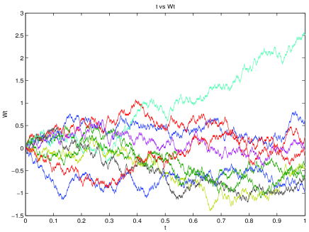
Figure 1: $(t,W_{t})$

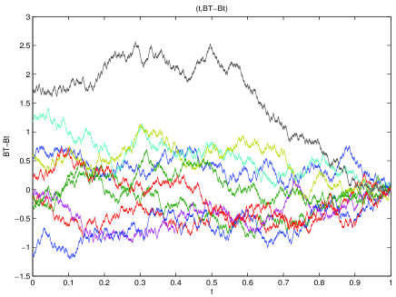
Figure 2: $(t,B_{T}-B_{t})$

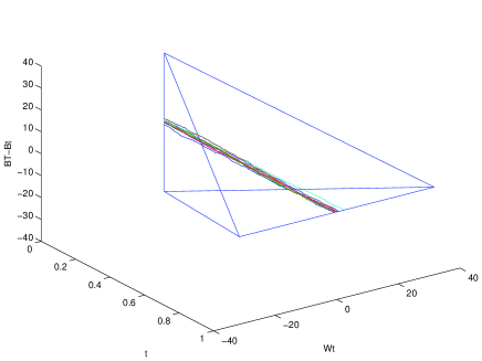
Figure 3: $(t,W_{t},B_{T}-B_{t})$

4 Main Results: Convergence Results for Discrete BDSDEs

4.1 Convergence of The Solution for Discrete BDSDEs

We consider the discrete terminal condition is $y_{n}^{n}:=\xi^{n}=\Phi((W_{j}^{n}),0\leq j\leq n)$, which is $\mathcal{G}_{nn}^{n}$-measurable random variable, for the discrete case. Firstly, for the scheme $(\ref{equation:discreteBDSDE})$ of BDSDE, if we construct the processes:

$$y_{t}^{n}=y_{[t/\delta]}^{n},z_{t}^{n}=z_{[t/\delta]}^{n},0\leq t\leq T$$

then the convergence between $(y_{t}^{n},z_{t}^{n})$ to $(y_{t},z_{t})$ can be derived in the same way as Donsker-Type theorem for BSDEs , by (P.Briand, B. Delyon and J. Mémin. (2001)PBJ ),

Assumption $(H.2)$ $\xi$ is $\mathcal{F}_{t}$-measurable and, for all $n,\xi^{n}$ is $\mathcal{G}_{nn}^{n}$-measurable s.t.

$$\mathbb{E}[\xi^{2}]+\sup\limits_{n}\mathbb{E}[(\xi^{n})^{2}]<\infty$$

Assumption $(H.3)$ $\xi^{n}$ converges to $\xi$ in $L^{1}$ as $n\rightarrow\infty.$

Theorem 4.1.

If the assumptions $(H.1)$, $(H.2)$ and $(H.3)$ hold. Let us consider the scaled random walks $B_{n},W_{n}$, if $B_{n}\rightarrow B,W_{n}\rightarrow W$ as $n\rightarrow\infty$ in the sense of that

$$\lim\limits_{n\rightarrow\infty}\sup\limits_{0\leq t\leq T}\left|B_{t}-B_{t}^{n}\right|=0\qquad\textrm{in }\mathbf{P},$$

and

$$\lim\limits_{n\rightarrow\infty}\sup\limits_{0\leq t\leq T}\left|W_{t}-W_{t}^{n}\right|=0\qquad\textrm{in }\mathbf{P},$$

then we have $(y^{n},z^{n})\rightarrow(y,z)$ in the following sense:

$$\lim\limits_{n\rightarrow\infty}\left\{\sup\limits_{0\leq t\leq T}\left|y_{t}^{n}-y_{t}\right|^{2}+\int\limits_{0}^{T}\left|z_{s}^{n}-z_{s}\right|^{2}ds\right\}=0\qquad\textrm{in }\mathbf{P}.$$ (12)

Method for the proof. The key point is to use the following decomposition

$$Y^{n}-Y=(Y^{n}-Y^{n,p})+(Y^{n,p}-Y^{\infty,p})+(Y^{\infty,p}-Y),$$ (13)

$$Z^{n}-Z=(Z^{n}-Z^{n,p})+(Z^{n,p}-Z^{\infty,p})+(Z^{\infty,p}-Z),$$ (14)

where the superscript $p$ stands for the approximation of the solution to the BDSDE via the Picard method. More precisely, we set $Y^{\infty,0}=0,Z^{\infty,0}=0,Y^{n,0}=0,Z^{n,0}=0$ and define $(Y^{\infty,p+1},Z^{\infty,p+1})$ as the solution of the BDSDE

$$Y_{t}^{\infty,p+1}=\xi+\int\limits_{t}^{T}f(Y_{s}^{\infty,p},Z_{s}^{\infty,p})ds+\int\limits_{t}^{T}g(Y_{s}^{\infty,p},Z_{s}^{\infty,p})dB_{s}-\int\limits_{t}^{T}Z_{s}^{\infty,p+1}dW_{s},\quad 0\leq t\leq T.$$ (15)

($(Y^{\infty,p+1},Z^{\infty,p+1})$ is solution of a BDSDE with non-dependent but random coefficients) and similarly

$$y_{k}^{n,p+1} = y_{k+1}^{n,p+1}+f(y_{k}^{n,p},z_{k}^{n,p})\delta+g(y_{k+1}^{n,p},z_{k+1}^{n,p})\sqrt{\delta}\varepsilon_{k+1}-z_{k}^{n,p+1}\sqrt{\delta}\beta_{k+1},\ k=n-1,...,0,{}$$

$$y_{n}^{n,p+1} = \xi^{n}$$ (16)

In order to define the discrete processes on $[0,T]$ we set for $0\leq t\leq T$, $Y_{t}^{n,p}=y_{[t/\delta]}^{n,p}$ and $Z_{t}^{n,p}=z_{[t/\delta]}^{n,p}$ so that $Y^{n,p}$ is càdlàg and $Z^{n,p}$ càglàd (càdlàg means right continuous with left limits and càglàd means left continuous with right limits).

We shall prove in Lemma 4.3 that the convergence of $(Y^{n,p},Z^{n,p})$ to $(Y^{n},Z^{n})$ is uniform in $n$ for the classical norm used for BDSDEs which is stronger than the convergence in the sense of $(\ref{equation:convergence1})$; this part is standard manipulations.

We shall prove that for any $p$, the convergence of $(Y^{n,p},Z^{n,p})$ to $(Y^{\infty,p},Z^{\infty,p})$ holds in the sense of $(\ref{equation:convergence1})$; this is the difficult part of the proof, and we shall need the results of section 4.1.1.

4.1.1 Convergence of Filtrations

Let us consider a sequence of càdlàg processes $W^{n}=(W_{t}^{n})_{0\leq t\leq T}$ and $W=(W_{t})_{0\leq t\leq T}$ a Brownian motion, all defined on the same probability space $(\Omega,\mathcal{F},\mathbf{P})$; $T$ is finite. We denote by $(\mathcal{G}_{t}^{n})$ (resp. $(\mathcal{G}_{t})$) the right continuous filtration s.t. $\sigma(W^{n})\subset\mathcal{G}^{n}_{t}$(resp.$\sigma(W)\subset\mathcal{G}_{t}$). Let us consider finally a sequence $X^{n}$ of $\mathcal{G}_{T}^{n}$-measurable integrable random variables, and $X$ an $\mathcal{G}_{T}$-measurable integrable random variable, together with the càdlàg martingales

$$M_{t}^{n}=\mathbb{E}[X^{n}\mid\mathcal{G}_{t}^{n}],\qquad M_{t}=\mathbb{E}[X\mid\mathcal{G}_{t}]$$

We denote by $[M^{n},M^{n}]$ (resp. $[M,M]$) the quadratic variation of $M^{n}$ (resp. $M$) and by $[M^{n},W^{n}]$ (resp. $[M,W]$) the cross variation of $M^{n}$ and $W^{n}$ (resp. $M$ and $W$).

Theorem 4.2.

Let us consider the following assumptions

(A1) for each $n$, $W^{n}$ is a square integrable $\mathcal{G}^{n}$-martingale with independent increments;

(A2) $W^{n}\rightarrow W$ in probability for the topology of uniform convergence of càdlàg processes indexed by $t\in[0,T]$;

(A3) a. $\mathbb{E}\left|X^{2}\right|+\sup\limits_{n}\mathbb{E}\left|(X^{n})^{2}\right|<\infty$

b. $\mathbb{E}[\left|X^{n}-X\right|]\rightarrow 0;$

Then, if conditions (A1) to (A3) are satisfied, we get

$$(W^{n},M^{n},[M^{n},M^{n}],[M^{n},W^{n}])\rightarrow(W,M,[M,M],[M,W])\qquad\textrm{in }\mathbf{P}$$

for the topology of uniform convergence on $[0,T]$. Moreover, for each $t\in[0,T]$, for each $0<\delta<1$,

$$(W_{t}^{n},M_{t}^{n},[M^{n},M^{n}]_{t}^{1/2},[M^{n},W^{n}]_{t}^{1/2})\rightarrow(W_{t},M_{t},[M,M]_{t}^{1/2},[M,W]_{t}^{1/2})\textrm{ in }L^{1+\delta}(\Omega,\mathcal{F},\mathbf{P}).$$

Corollary 4.1.

Let $W$ and $W^{n}$, $n\in\mathbb{N}^{\ast}$, be the standard Brownian motion and the random walks of Theorem 4.1 Let us consider, on the same space, $X$ and $X^{n}$ satisfying the assumption (A3) of Theorem 4.2.

Then there exists a sequence $(Z_{t}^{n})_{0\leq t\leq T}$ of $\mathcal{G}_{\cdot}^{n}$-progressively measurable processes, and an $\mathcal{G}_{\cdot}$-progressively measurable process $(Z_{t})_{0\leq t\leq T}$ such that: for all $t\in[0,T]$,

$$M_{t}^{n}=\mathbb{E}[X^{n}]+\int\limits_{0}^{t}Z_{s}^{n}dW_{s}^{n},\qquad M_{t}=\mathbb{E}[X]+\int\limits_{0}^{t}Z_{s}dW_{s}$$

and

$$\int\limits_{0}^{T}(Z_{t}^{n}-Z_{t})^{2}ds\rightarrow 0\qquad\textrm{in }\mathbf{P}.$$

Moreover, if $0<\delta<1$, $Z^{n}$ converges to $Z$ in the space $L^{1+\delta}(\Omega\times[0,T],\mathcal{F}\times\mathcal{B}([0,T]),\mathbf{P}\mathscr{\otimes\lambda})$ where $\lambda$ denotes the Lebesgue measure on $([0,T],\mathcal{B([}0,T\mathcal{]))}$.

4.1.2 Proof of Theorem 4.1

Equations $(\ref{equation:decompositonY}),(\ref{equation:decompositonZ})$ with the following lemma proved in appendix A.

Lemma 4.3.

Here we need to assume that

$$\lim\limits_{n\rightarrow\infty}\sup\limits_{0\leq t\leq T}\left|B_{t}-B_{t}^{n}\right|=0\qquad\textrm{in }\mathbf{P}.$$

With the notations following $(\ref{equation:continuousPicard}),(\ref{equation:discretePicard}),$

$$\sup\limits_{n}\mathbb{E}[\sup\limits_{0\leq t\leq T}\left|Y_{t}^{n}-Y_{t}^{n,p}\right|^{2}+\int\limits_{0}^{T}\left|Z_{s}^{n}-Z_{s}^{n,p}\right|^{2}ds]\rightarrow 0,\ as\ p\rightarrow\infty$$

imply that it remains to prove the convergence to zero of the process $Y^{n,p}-Y^{\infty,p}$and $Z^{n,p}-Z^{\infty,p}.$ This will be done by induction on $p.$ For sake of clarity, we drop the superscript $p,$set the time in subscript and write everything in continuous time, so that $(\ref{equation:continuousPicard}),(\ref{equation:discretePicard})$ become

$$Y_{t}^{\prime}=\xi+\int\limits_{t}^{T}f(Y_{s},Z_{s})ds+\int\limits_{t}^{T}g(Y_{s},Z_{s})dB_{s}-\int\limits_{t}^{T}Z_{s}^{\prime}dW_{s},\qquad 0\leq t\leq T.$$

$$Y_{t}^{\prime n}=\xi^{n}+\int\limits_{t}^{T}f(Y_{s-}^{n},Z_{s}^{n})dA_{s}^{n}+\int\limits_{t}^{T}g(Y_{s-}^{n},Z_{s}^{n})dB_{s}^{n}-\int\limits_{t}^{T}Z_{s}^{\prime n}dW_{s}^{n},\qquad 0\leq t\leq T.$$

where $A_{s}^{n}=[s/\delta]\delta$ and $Y_{-}$ denotes the càglàd process associated to $Y$. The assumption is that $\{Y_{t}^{n},Z_{t}^{n}\}_{0\leq t\leq T}$ converges to $\{Y_{t},Z_{t}\}_{0\leq t\leq T}$ in sense of $(\ref{equation:convergence1})$ and we have to prove that $\{Y_{t}^{\prime n},Z_{t}^{\prime n}\}_{0\leq t\leq T}$ converges to $\{Y_{t}^{\prime},Z_{t}^{\prime}\}_{0\leq t\leq T}$ in the same sense.

According to the Peng and Pardoux’s paper PP , we define the filtration $(\mathcal{G}_{t})_{0\leq t\leq T}$ by

$$\mathcal{G}_{t}\doteq\mathcal{F}_{t}^{W}\vee\mathcal{F}_{T}^{B}$$

and the $\mathcal{G}_{t}$-square integrable martingale

$$M_{t}=\mathbb{E}^{\mathcal{G}_{t}}[\xi+\int\limits_{0}^{T}f(Y_{s},Z_{s})ds+\int\limits_{0}^{T}g(Y_{s},Z_{s})dB_{s}],\qquad 0\leq t\leq T.$$

Then there exists $\mathcal{G}_{t}$-progressively measurable process $\{Z_{t}^{\prime}\}$ such that

$$\mathbb{E}\int\limits_{0}^{T}\left|Z_{t}^{\prime}\right|^{2}dt<\infty$$

$$M_{t}=M_{0}+\int\limits_{0}^{t}Z_{s}^{\prime}dW_{s},\qquad 0\leq t\leq T.$$

On the other hand, the process, defined by

$$M_{t}^{n}=Y_{t}^{\prime n}+\int\limits_{0}^{t}f(Y_{s-}^{n},Z_{s}^{n})dA_{s}^{n}+\int\limits_{0}^{t}g(Y_{s-}^{n},Z_{s}^{n})dB_{s}^{n},\qquad 0\leq t\leq T,$$ (17)

satisfies

$$M_{t}^{n}=M_{0}^{n}+\int\limits_{0}^{t}Z_{s}^{\prime n}dW_{s}^{n}.$$ (18)

Hence $M^{n}$ is an $\mathcal{F}_{\cdot}^{n}$-martingale and, since $Y_{T}^{n}=\xi^{n},$

$$M_{t}^{n}=\mathbb{E}[M_{T}^{n}\mid\mathcal{G}_{t}^{n}],\qquad M_{T}^{n}=Y_{t}^{n}+\int\limits_{0}^{T}f(Y_{s-}^{n},Z_{s}^{n})dA_{s}^{n}+\int\limits_{0}^{T}g(Y_{s-}^{n},Z_{s}^{n})dB_{s}^{n}.$$ (19)

If we want to apply Corollary, we have to prove the $L^{1}$ convergence of $M_{T}^{n}$. But since $Y^{n}$ and $Z^{n}$ are piecewise constant, we have

$$\begin{array}[]{llllll}&&\left|M_{T}^{n}-Y_{T}-\int\limits_{0}^{T}f(Y_{s},Z_{s})ds-\int\limits_{0}^{T}g(Y_{s},Z_{s})dB_{s}\right|\\ &\leq&\left|Y_{T}^{n}-Y_{T}\right|+\int\limits_{0}^{T}\left|f(Y_{s}^{n},Z_{s}^{n})-f(Y_{s},Z_{s})\right|ds+\left|\int\limits_{0}^{T}g(Y_{s}^{n},Z_{s}^{n})dB_{s}^{n}-\int\limits_{0}^{T}g(Y_{s},Z_{s})dB_{s}\right|\\ &\leq&(1+KT)\sup\limits_{0\leq t\leq T}\left|Y_{t}^{n}-Y_{t}\right|+K\int\limits_{0}^{T}\left|Z_{s}^{n}-Z_{s}\right|ds+\left|\int\limits_{0}^{T}(g(Y_{s}^{n},Z_{s}^{n})-g(Y_{s},Z_{s}))dB_{s}\right|\\ &&+\left|\int\limits_{0}^{T}g(Y_{s}^{n},Z_{s}^{n})d(B_{s}^{n}-B_{s})\right|\\ &\leq&(1+KT)\sup\limits_{0\leq t\leq T}\left|Y_{t}^{n}-Y_{t}\right|+K\int\limits_{0}^{T}\left|Z_{s}^{n}-Z_{s}\right|ds+K\sqrt{T}\sup\limits_{0\leq t\leq T}\left|Y_{t}^{n}-Y_{t}\right|\\ &&+\left|\int\limits_{0}^{T}(K\left|Y_{s}^{n}\right|+\alpha\left|Z_{s}^{n}\right|+\left|g(0,0)\right|)d(B_{s}^{n}-B_{s})\right|\end{array}$$

which tends to zero in probability and then in $L^{1}$ by $L^{2}$-bounded. This and equations $(\ref{representation of Martingale}),$ $(\ref{Martingale})$, imply together with Corollary that $M^{n}$ converges to

$$M_{t}=\mathbb{E}^{\mathcal{G}_{t}}[\xi+\int\limits_{0}^{T}f(Y_{s},Z_{s})ds+\int\limits_{0}^{T}g(Y_{s},Z_{s})dB_{s}]=Y_{t}^{\prime}+\int\limits_{0}^{t}f(Y_{s},Z_{s})ds+\int\limits_{0}^{t}g(Y_{s},Z_{s})dB_{s}$$

in the sense that

$$\sup\limits_{0\leq t\leq T}\left|M_{t}^{n}-M_{t}\right|+\int\limits_{0}^{T}\left|Z_{s}^{\prime n}-Z_{s}\right|^{2}ds\rightarrow 0\qquad\textrm{in }\mathbf{P}.$$

Since we want to prove that

$$\sup\limits_{0\leq t\leq T}\left|Y_{t}^{\prime n}-Y_{t}^{\prime}\right|+\int\limits_{0}^{T}\left|Z_{s}^{\prime n}-Z_{s}\right|^{2}ds\rightarrow 0\qquad\textrm{in }\mathbf{P},$$

it remain only to demonstrate

$$\sup\limits_{0\leq t\leq T}\left|\int\limits_{0}^{t}f(Y_{s}^{n},Z_{s}^{n})dA_{s}^{n}-\int\limits_{0}^{t}f(Y_{s},Z_{s})ds+\int\limits_{0}^{t}g(Y_{s-}^{n},Z_{s}^{n})dB_{s}^{n}-\int\limits_{0}^{t}g(Y_{s},Z_{s})dB_{s}\right|\rightarrow 0\quad\textrm{in }\mathbf{P}.$$

This is true since we have just proved the convergence of $\int\limits_{0}^{T}\left|f(Y_{s}^{n},Z_{s}^{n})-f(Y_{s},Z_{s})\right|ds$ to zero in probability and since the jumps of $t\rightarrow\int\limits_{0}^{t}f(Y_{s}^{n},Z_{s}^{n})dA_{s}^{n}$ tends to zero according to

$$\sup\limits_{0\leq t\leq T}\left|\int\limits_{0}^{t}Z_{s}^{n}dA_{s}^{n}-\int\limits_{0}^{t}Z_{s}ds\right|\rightarrow 0\quad\textrm{in }\mathbf{P},\quad\sup\limits_{0\leq t\leq T}\left|\int\limits_{0}^{t}(Z_{s}^{n})^{2}dA_{s}^{n}-\int\limits_{0}^{t}Z_{s}^{2}ds\right|\rightarrow 0\quad\textrm{in }\mathbf{P},$$

while we also have proved the convergence of $\left|\int\limits_{0}^{T}g(Y_{s}^{n},Z_{s}^{n})dB_{s}^{n}-\int\limits_{0}^{T}g(Y_{s},Z_{s})dB_{s}\right|$ to zero in probability.

4.2 Convergence of Modified Solution

Theorem 4.4.

If the assumptions $(H.1)$, $(H.2)$ and $(H.3)$ hold. We also assume that

$$\lim\limits_{n\rightarrow\infty}\sup\limits_{0\leq t\leq T}\left|B_{t}-B_{t}^{n}\right|=0\qquad\textrm{in }\mathbf{P}.$$

Then the discrete solutions $\{(\overline{y}^{n},\overline{z}^{n})\}_{n=1}^{\infty}$ under the scheme $(\ref{equation:modifieddiscreteBDSDE})$ converge to the solution $(y,z)$ of $(\ref{equation:BDSDE})$ in the following senses:

$$\lim\limits_{n\rightarrow\infty}\left\{\sup\limits_{0\leq t\leq T}\left|\overline{y}_{t}^{n}-y_{t}\right|^{2}+\int\limits_{0}^{T}\left|\overline{z}_{s}^{n}-z_{s}\right|^{2}ds\right\}=0\qquad\textrm{in }\mathbf{P}.$$ (20)

This can be derived from the convergence $(\ref{equation:convergence1}).$

For the convergence of this scheme, we must consider the following estimates under the following:

Assumption $\xi^{n}\in L^{2}(\xi_{n}^{n})$, $\mathbb{E}[\sum\limits_{j=0}^{n}\left|f(0,0)\right|^{2}]<\infty$, $\mathbb{E}[\sum\limits_{j=0}^{n}\left|g(0,0)\right|^{2}]<\infty.$

For this reason, we need the following Gronwall type lemma, which is proved in MPX .

Lemma 4.5.

Let us consider $a,b,\alpha$ positive constant, $b\delta<1$ and a sequence $(v_{j})_{j=1,...,n}$ of positive numbers such that, for every $k$

$$v_{j}+\alpha\leq a+b\delta\sum\limits_{i=1}^{j}v_{i},$$ (21)

then

$$\sup\limits_{j\leq n}v_{j}+\alpha\leq a\varepsilon_{\delta}(b),$$ (22)

where $\varepsilon_{\delta}(b)$ is the convergent sequence:

$$\varepsilon_{\delta}(b)=1+\sum\limits_{p=1}^{\infty}\frac{b^{p}}{p!}(1+\delta)\cdot\cdot\cdot(1+(p-1)\delta)$$ (23)

which is decreasing in $\delta$ and tends to $e^{b}$ as $\delta\rightarrow\infty.$

Lemma 4.6.

We assume that $\delta$ is small enough such that $(1+2K+7K^{2})\delta<1$. Then

$$\sup\limits_{j}\mathbb{E}\left|\overline{y}_{j}^{n}\right|^{2}+\delta\mathbb{E}[\sum\limits_{j=0}^{n}\left|\overline{z}_{j}^{n}\right|^{2}]\leq C_{\xi^{n},f,g}e^{(1+2K+7K^{2})T}$$ (24)

where $C_{\xi^{n},f,g}=\left|f(0,0)\right|^{2}+3\left|g(0,0)\right|^{2}+(1+K\delta+3K^{2}\delta+3\alpha^{2}\sqrt{\delta})\mathbb{E}\left|\xi^{n}\right|^{2}.$

Proof. By explicit scheme, we have

$$\overline{y}_{j}^{n}=\overline{y}_{j+1}^{n}+f(\mathbb{E}[\overline{y}_{j+1}^{n}\mid\mathcal{G}_{jj}^{n}],\overline{z}_{j}^{n})\delta+g(\overline{y}_{j+1}^{n},\overline{z}_{j+1}^{n})\sqrt{\delta}\varepsilon_{j+1}-\overline{z}_{j}^{n}\sqrt{\delta}\beta_{j+1}.$$

We then have

$$\begin{array}[]{ll}\mathbb{E}\left|\overline{y}_{j}^{n}\right|^{2}-\mathbb{E}\left|\overline{y}_{j+1}^{n}\right|^{2}=-\mathbb{E}\left|\overline{z}_{j}^{n}\right|^{2}\delta+\mathbb{E}[g(\overline{y}_{j+1}^{n},\overline{z}_{j+1}^{n})]^{2}\delta-\mathbb{E}\left|f(E[\overline{y}_{j+1}^{n}\mid\mathcal{G}_{jj}^{n}],\overline{z}_{j}^{n})\right|^{2}\delta^{2}\\ \hskip 105.27519pt+2\mathbb{E}[\overline{y}_{j}^{n}\cdot f(\mathbb{E}[\overline{y}_{j+1}^{n}\mid\mathcal{G}_{jj}^{n}],\overline{z}_{j}^{n})]\delta.\end{array}$$ (25)

Taking sum for $j=i,...,n-1$ yields

$$\mathbb{E}\left|\overline{y}_{i}^{n}\right|^{2} \leq \mathbb{E}\left|\xi^{n}\right|^{2}-\sum\limits_{j=i}^{n-1}\mathbb{E}\left|\overline{z}_{j}^{n}\right|^{2}\delta+2\delta\mathbb{E}\sum\limits_{j=i}^{n-1}\{\left|\overline{y}_{j}^{n}\right|(\left|f(0,0)\right|+K\left|\mathbb{E}[\overline{y}_{j+1}^{n}\mid\mathcal{G}_{jj}^{n}]\right|+K\left|\overline{z}_{j}^{n}\right|)\}$$

$$+\delta\mathbb{E}\sum\limits_{j=i}^{n-1}(\left|g(0,0)\right|+K\left|\overline{y}_{j+1}^{n}\right|+\alpha\left|\overline{z}_{j+1}^{n}\right|)^{2}.$$

Since the second last term is dominated by

$$\delta\mathbb{E}\sum\limits_{j=i}^{n-1}\{\left|\overline{y}_{j}^{n}\right|^{2}(1+K+4K^{2})+\left|f(0,0)\right|^{2}+K\left|\mathbb{E}[\overline{y}_{j+1}^{n}\mid\mathcal{G}_{jj}^{n}]\right|^{2}+\frac{1}{4}\left|\overline{z}_{j}^{n}\right|^{2}\}$$

$$\leq\delta\mathbb{E}\sum\limits_{j=i}^{n-1}\{\left|\overline{y}_{j}^{n}\right|^{2}(1+K+4K^{2})+\left|f(0,0)\right|^{2}+\frac{1}{4}\left|\overline{z}_{j}^{n}\right|^{2}\}+K\delta\mathbb{E}\left|\xi^{n}\right|^{2}$$

and the last term is dominated by

$$3\delta\mathbb{E}\sum\limits_{j=i}^{n-1}(\left|g(0,0)\right|^{2}+K^{2}\left|\overline{y}_{j+1}^{n}\right|^{2}+\alpha^{2}\left|\overline{z}_{j+1}^{n}\right|^{2})\hskip 142.26378pt$$

$$\leq 3\delta\mathbb{E}\sum\limits_{j=i}^{n-1}(\left|g(0,0)\right|^{2}+K^{2}\left|\overline{y}_{j}^{n}\right|^{2}+\alpha^{2}\left|\overline{z}_{j}^{n}\right|^{2})+3(K^{2}\delta+\alpha^{2}\sqrt{\delta})\mathbb{E}\left|\xi^{n}\right|^{2},$$

we thus have

$$\mathbb{E}\left|\overline{y}_{j}^{n}\right|^{2}+\delta(\frac{3}{4}-3\alpha^{2})\sum\limits_{j=i}^{n-1}\mathbb{E}\left|\overline{z}_{j}^{n}\right|^{2} \leq \left|f(0,0)\right|^{2}+3\left|g(0,0)\right|^{2}+(1+K\delta+3K^{2}\delta$$

$$+3\alpha^{2}\sqrt{\delta})\mathbb{E}\left|\xi^{n}\right|^{2}+(1+2K+7K^{2})\delta\sum\limits_{j=i}^{n-1}\mathbb{E}\left|\overline{y}_{j}^{n}\right|^{2}.$$

Then by Lemma 4.5, we obtain $(\ref{equation:control of modified solution}).$

Proof of Theorem 4.4 The convergence of $(y^{n},z^{n})$ to $(y,z)$ is already proved above. To prove that of $(\overline{y}^{n},\overline{z}^{n})$, it is sufficient to prove

$$\lim\limits_{n\rightarrow\infty}\left\{\sup\limits_{0\leq t\leq T}\left|\overline{y}_{t}^{n}-y_{t}^{n}\right|^{2}+\int\limits_{0}^{T}\left|\overline{z}_{s}^{n}-z_{s}^{n}\right|^{2}ds\right\}=0.$$

From $(\ref{equation:discreteBDSDE})$ and $(\ref{equation:modifieddiscreteBDSDE}),$ we have

$$\mathbb{E}\left|\overline{y}_{j}^{n}-y_{j}^{n}\right|^{2} = \mathbb{E}\left|\overline{y}_{j+1}^{n}-y_{j+1}^{n}\right|^{2}-\delta\mathbb{E}\left|\overline{z}_{j}^{n}-z_{j}^{n}\right|^{2}+\delta\mathbb{E}\left|g(\overline{y}_{j+1}^{n},\overline{z}_{j+1}^{n})-g(y_{j+1}^{n},z_{j+1}^{n})\right|^{2}$$

$$-\mathbb{E}\left|f(y_{j}^{n},z_{j}^{n})-f(\mathbb{E}[\overline{y}_{j+1}^{n}\mid\mathcal{G}_{jj}^{n}],\overline{z}_{j}^{n})\right|^{2}\delta^{2}$$

$$+2\mathbb{E}[(\overline{y}_{j}^{n}-y_{j}^{n})\cdot(f(y_{j}^{n},z_{j}^{n})-f(\mathbb{E}[\overline{y}_{j+1}^{n}\mid\mathcal{G}_{jj}^{n}],\overline{z}_{j}^{n}))]\delta.$$

We then take sum over $i$ from $j$ to $n-1.$ With $\xi^{n}-\overline{\xi}^{n}=0,$ we have

$$\mathbb{E}\left|\overline{y}_{i}^{n}-y_{i}^{n}\right|^{2} \leq -\delta\mathbb{E}\sum\limits_{j=i}^{n-1}\left|\overline{z}_{j}^{n}-z_{j}^{n}\right|^{2}+\delta\sum\limits_{j=i}^{n-1}\mathbb{E}\left|g(\overline{y}_{j+1}^{n},\overline{z}_{j+1}^{n})-g(y_{j+1}^{n},z_{j+1}^{n})\right|^{2}$$

$$+2\delta\sum\limits_{j=i}^{n-1}\mathbb{E}[(\overline{y}_{j}^{n}-y_{j}^{n})\cdot(f(y_{j}^{n},z_{j}^{n})-f(\mathbb{E}[\overline{y}_{j+1}^{n}\mid\mathcal{G}_{jj}^{n}],\overline{z}_{j}^{n}))]$$

$$\leq -\delta\mathbb{E}\sum\limits_{j=i}^{n-1}\left|\overline{z}_{j}^{n}-z_{j}^{n}\right|^{2}+2K^{2}\delta\sum\limits_{j=i}^{n-1}\mathbb{E}\left|\overline{y}_{j+1}^{n}-y_{j+1}^{n}\right|^{2}+2\alpha^{2}\delta\sum\limits_{j=i}^{n-1}\mathbb{E}\left|\overline{z}_{j+1}^{n}-z_{j+1}^{n}\right|^{2}$$

$$+2K^{2}\delta\sum\limits_{j=i}^{n-1}\mathbb{E}\left|\overline{y}_{j}^{n}-y_{j}^{n}\right|^{2}+\delta/2\sum\limits_{j=i}^{n-1}\mathbb{E}\left|\overline{z}_{j}^{n}-z_{j}^{n}\right|^{2}$$

$$+2K\delta\mathbb{E}\sum\limits_{j=i}^{n-1}\left|\overline{y}_{i}^{n}-y_{i}^{n}\right|\cdot\left|y_{j}^{n}-\mathbb{E}[\overline{y}_{j+1}^{n}\mid\mathcal{G}_{jj}^{n}]\right|.$$

Since $y_{j}^{n}-\mathbb{E}[\overline{y}_{j+1}^{n}\mid\mathcal{G}_{jj}^{n}]=f(\mathbb{E}[\overline{y}_{j+1}^{n}\mid\mathcal{G}_{jj}^{n}],\overline{z}_{j}^{n})\delta+\sqrt{\delta}\mathbb{E}[g(\overline{y}_{j+1}^{n},\overline{z}_{j+1}^{n})\mid\mathcal{G}_{jj}^{n}]\varepsilon_{j+1}$, the last term is dominated by

$$(K^{2}\delta^{4}+\delta^{3} + 2K\delta^{2})\sum\limits_{j=i}^{n-1}\mathbb{E}\left|\overline{y}_{j}^{n}-y_{j}^{n}\right|^{2}+\sum\limits_{j=i}^{n-1}K^{2}\mathbb{E}\left|f(\mathbb{E}[\overline{y}_{j+1}^{n}\mid\mathcal{G}_{jj}^{n}],\overline{z}_{j}^{n})\right|^{2}\delta^{3}$$

$$+\sum\limits_{j=i}^{n-1}\mathbb{E}\left|\mathbb{E}[g(\overline{y}_{j+1}^{n},\overline{z}_{j+1}^{n})\mid\mathcal{G}_{jj}^{n}]\right|^{2}\delta.$$

But with $(\ref{equation:control of modified solution})$, the second term is bounded by $C\delta^{2}$, and the last term is bounded by

$$4K^{2}\delta\sum\limits_{j=i}^{n-1}\mathbb{E}\left|\overline{y}_{j}^{n}\right|^{2}+4\alpha^{2}\delta\sum\limits_{j=i}^{n-1}\mathbb{E}\left|\overline{z}_{j}^{n}\right|^{2}+4(K^{2}\delta+\alpha^{2}\sqrt{\delta})\mathbb{E}\left|\xi^{n}\right|^{2}+2\left|g(0,0)\right|^{2}.$$

We thus have

$$\mathbb{E}\left|\overline{y}_{i}^{n}-y_{i}^{n}\right|^{2}+(\frac{1}{2}-2\alpha^{2})\delta\mathbb{E}\sum\limits_{j=i}^{n-1}\left|\overline{z}_{j}^{n}-z_{j}^{n}\right|^{2} \leq (4K^{2}\delta+K^{2}\delta^{4}+\delta^{3}+2K\delta^{2})\sum\limits_{j=i}^{n-1}\mathbb{E}\left|\overline{y}_{j}^{n}-y_{j}^{n}\right|^{2}$$

$$+4K^{2}\delta\sum\limits_{j=i}^{n-1}\mathbb{E}\left|\overline{y}_{j}^{n}\right|^{2}+4\alpha^{2}\delta\sum\limits_{j=i}^{n-1}\mathbb{E}\left|\overline{z}_{j}^{n}\right|^{2}$$

$$+4(K^{2}\delta+\alpha^{2}\sqrt{\delta})\mathbb{E}\left|\xi^{n}\right|^{2}+2\left|g(0,0)\right|^{2}+C\delta^{2}.$$

According to Lemma 4.6 and here providing that $g(0,0)=0$, we further have

$$\mathbb{E}\left|\overline{y}_{i}^{n}-y_{i}^{n}\right|^{2}+(\frac{1}{2}-2\alpha^{2})\delta\mathbb{E}\sum\limits_{j=i}^{n-1}\left|\overline{z}_{j}^{n}-z_{j}^{n}\right|^{2} \leq (1+2k+5k^{2})\delta\sum\limits_{j=i}^{n-1}\mathbb{E}\left|\overline{y}_{j}^{n}-y_{j}^{n}\right|^{2}+C^{\prime}\sqrt{\delta}.$$

By Gronwall Lemma 4.2.2, we get

$$\sup\limits_{i\leq n}\mathbb{E}\left|\overline{y}_{i}^{n}-y_{i}^{n}\right|^{2}\leq C^{\prime}\sqrt{\delta}e^{(1+2k+5k^{2})T}.$$

Then these two inequalities implies (20).

Appendix A. Proof of Lemma 4.3

For the proof of this lemma we come back to the discrete notations and we show that
Lemma A.1 There exist $\alpha>1$ and $n_{0}\in\mathbb{N}$ such that for all $n\geq n_{0}$, for all $p\in\mathbb{N}^{*}$,

$$\left\|(y^{n,p+1}-y^{n,p},z^{n,p+1}-z^{n,p})\right\|_{\alpha}^{2}\leq\frac{2}{3}\left\|(y^{n,p}-y^{n,p-1},z^{n,p}-z^{n,p-1})\right\|_{\alpha}^{2},$$

where, for $p\in\mathbb{N}$,

$$\left\|(y^{n,p+1}-y^{n,p},z^{n,p+1}-z^{n,p})\right\|_{\alpha}^{2}:=\mathbb{E}\left[\sup\limits_{0\leq k\leq n}\alpha^{k\delta}\left|y_{k}^{n,p+1}-y_{k}^{n,p}\right|^{2}+\delta\sum\limits_{k=0}^{n-1}\alpha^{k\delta}\left|z_{k}^{n,p+1}-z_{k}^{n,p}\right|^{2}\right].$$

Proof. For notational convenience, let us write $y,z$ in place of $y^{n,p+1}-y^{n,p},$ $z^{n,p+1}-z^{n,p}$ and $u,v$ in place of $y^{n,p}-y^{n,p-1},$ $z^{n,p}-z^{n,p-1}$. Let us pick $\varphi>1$ to be chosen later. With these notations in hands, we have, for $k=0,...,n-1$, since $y_{n}=0,$

$$\varphi^{k}y_{k}^{2}=\sum\limits_{i=k}^{n-1}\left(\varphi^{i}y_{i}^{2}-\varphi^{i+1}y_{i+1}^{2}\right)=(1-\varphi)\sum\limits_{i=k}^{n-1}\varphi^{i}y_{i}^{2}+\varphi\sum\limits_{i=k}^{n-1}\varphi^{i}(y_{i}^{2}-y_{i+1}^{2}).$$

We write $y_{i}^{2}-y_{i+1}^{2}=2y_{i}(y_{i}-y_{i+1})-(y_{i}-y_{i+1})^{2},$ to use the equation $(\ref{equation:discretePicard}),$ since

$$y_{i}-y_{i+1} = \delta\{f(y_{i}^{n,p},z_{i}^{n,p})-f(y_{i}^{n,p-1},z_{i}^{n,p-1})\}+\sqrt{\delta}\{g(y_{i+1}^{n,p},z_{i+1}^{n,p})-g(y_{i+1}^{n,p-1},z_{i+1}^{n,p-1})\}\varepsilon_{i+1}$$ (A.1)

$$-\sqrt{\delta}z_{i}\beta_{i+1}.$$

According to $(H.1),$ we have, for each $\nu>0,$

$$2y_{i}\{f(y_{i}^{n,p},z_{i}^{n,p})-f(y_{i}^{n,p-1},z_{i}^{n,p-1})\} \leq 2K\left|y_{i}\right|(\left|u_{i}\right|+\left|v_{i}\right|)$$

$$\leq 2(K^{2}/\nu)y_{i}^{2}+\nu(u_{i}^{2}+v_{i}^{2}),$$

$$2y_{i}\{g(y_{i+1}^{n,p},z_{i+1}^{n,p})-g(y_{i+1}^{n,p-1},z_{i+1}^{n,p-1})\} \leq 2\left|y_{i}\right|(K\left|u_{i+1}\right|+\alpha\left|v_{i+1}\right|)$$

$$\leq [(K^{2}+\alpha^{2})/\nu]y_{i}^{2}+\nu(u_{i+1}^{2}+v_{i+1}^{2})$$

and moreover, $(A.1)$ implies easily that

$$\delta z_{i}^{2}\leq 3(y_{i}-y_{i+1})^{2}+6K^{2}\delta^{2}(u_{i}^{2}+v_{i}^{2})-6\delta(K^{2}u_{i+1}^{2}+\alpha^{2}v_{i+1}^{2}).$$

As a byproduct of these inequalities, we deduce that, for $k=0,...,n-1,$

$$2\sum\limits_{i=k}^{n-1}\varphi^{i}y_{i}(y_{i}-y_{i+1})$$

$$\leq 2K^{2}(\delta/\nu)\sum\limits_{i=k}^{n-1}\varphi^{i}y_{i}^{2}+\nu\delta\sum\limits_{i=k}^{n-1}\varphi^{i}(u_{i}^{2}+v_{i}^{2})+[\sqrt{\delta}(K^{2}+\alpha^{2})/\nu]\sum\limits_{i=k}^{n-1}\varphi^{i}y_{i}^{2}\varepsilon_{i+1}$$

$$+\nu\sqrt{\delta}\sum\limits_{i=k}^{n-1}\varphi^{i}(u_{i+1}^{2}+v_{i+1}^{2})\varepsilon_{i+1}-2\sqrt{\delta}\sum\limits_{i=k}^{n-1}\varphi^{i}y_{i}z_{i}\beta_{i+1},$$

$$-\sum\limits_{i=k}^{n-1}\varphi^{i}(y_{i}^{2}-y_{i+1}^{2})\leq-(\delta/3)\sum\limits_{i=k}^{n-1}\varphi^{i}z_{i}^{2}+2K^{2}\delta^{2}\sum\limits_{i=k}^{n-1}\varphi^{i}(u_{i}^{2}+v_{i}^{2})-2\delta\sum\limits_{i=k}^{n-1}\varphi^{i}(K^{2}u_{i+1}^{2}+\alpha^{2}v_{i+1}^{2}),$$

and, setting $\rho=(\nu+2K^{2}\delta)\varphi\delta,$ we get

$$\varphi^{k}y_{k}^{2}+\varphi(\delta/3)\sum\limits_{i=k}^{n-1}\varphi^{i}z_{i}^{2} \leq (1-\varphi+2K^{2}\delta\varphi/\nu)\sum\limits_{i=k}^{n-1}\varphi^{i}y_{i}^{2}+\rho\sum\limits_{i=k}^{n-1}\varphi^{i}(u_{i}^{2}+v_{i}^{2})$$

$$+[\sqrt{\delta}\varphi(K^{2}+\alpha^{2})/\nu]\sum\limits_{i=k}^{n-1}\varphi^{i}y_{i}^{2}\varepsilon_{i+1}+\nu\varphi\sqrt{\delta}\sum\limits_{i=k}^{n-1}\varphi^{i}(u_{i+1}^{2}+v_{i+1}^{2})\varepsilon_{i+1}$$

$$-2\delta\varphi\sum\limits_{i=k}^{n-1}\varphi^{i}(K^{2}u_{i+1}^{2}+\alpha^{2}v_{i+1}^{2})-2\varphi\sqrt{\delta}\sum\limits_{i=k}^{n-1}\varphi^{i}y_{i}z_{i}\beta_{i+1}.$$

Thus, if $1-\varphi+2K^{2}\delta\varphi/\nu\leq 0$, we have, for $k=0,...,n-1,$

$$\begin{array}[]{ll}\varphi^{k}y_{k}^{2}+\varphi(\delta/3)\sum\limits_{i=k}^{n-1}\varphi^{i}z_{i}^{2}\\ \leq\rho\sum\limits_{i=k}^{n-1}\varphi^{i}(u_{i}^{2}+v_{i}^{2})+[\sqrt{\delta}\varphi(K^{2}+\alpha^{2})/\upsilon]\sum\limits_{i=k}^{n-1}\varphi^{i}y_{i}^{2}\varepsilon_{i+1}\\ +\nu\varphi\sqrt{\delta}\sum\limits_{i=k}^{n-1}\varphi^{i}(u_{i+1}^{2}+v_{i+1}^{2})\varepsilon_{i+1}-2\varphi\sqrt{\delta}\sum\limits_{i=k}^{n-1}\varphi^{i}y_{i}z_{i}\beta_{i+1}.\end{array}$$ (A.2)

In particular, taking the expectation of the previous inequality for $k=0$, we get

$$\mathbb{E}[\sum\limits_{i=0}^{n-1}\varphi^{i}z_{i}^{2}]\leq 3(\nu+2K^{2}\delta)\mathbb{E}[\sum\limits_{i=0}^{n-1}\varphi^{i}(u_{i}^{2}+v_{i}^{2})].$$ (A.3)

Now, coming back to $(A.2),$ we have, since $y_{n}=0,$

$$\sup\limits_{0\leq k\leq n}\varphi^{k}y_{k}^{2} \leq \rho\sum\limits_{i=0}^{n-1}\varphi^{i}(u_{i}^{2}+v_{i}^{2})+2[\sqrt{\delta}\varphi(K^{2}+\alpha^{2})/\nu]\sup\limits_{0\leq k\leq n-1}\left|\sum\limits_{i=0}^{n-1}\varphi^{i}y_{i}^{2}\varepsilon_{i+1}\right|$$

$$+2\nu\varphi\sqrt{\delta}\sup\limits_{0\leq k\leq n-1}\left|\sum\limits_{i=0}^{n-1}\varphi^{i}(u_{i+1}^{2}+v_{i+1}^{2})\varepsilon_{i+1}\right|+4\varphi\sqrt{\delta}\sup\limits_{0\leq k\leq n-1}\left|\sum\limits_{i=0}^{n-1}\varphi^{i}y_{i}z_{i}\beta_{i+1}\right|$$

and using Burkholder-Davis-Gundy inequality, we obtain,

$$\mathbb{E}[\sup\limits_{0\leq k\leq n}\varphi^{k}y_{k}^{2}] \leq \rho\mathbb{E}[\sum\limits_{i=0}^{n-1}\varphi^{i}(u_{i}^{2}+v_{i}^{2})]+C_{1}[\sqrt{\delta}\varphi(K^{2}+\alpha^{2})/\nu]\mathbb{E}[(\sum\limits_{i=0}^{n-1}\varphi^{2i}y_{i}^{4})^{1/2}]$$

$$+C_{2}\nu\varphi\sqrt{\delta}\mathbb{E}[(\sum\limits_{i=0}^{n-1}\varphi^{2i}(u_{i+1}^{2}+v_{i+1}^{2})^{2})^{1/2}]+C_{3}\varphi\sqrt{\delta}\mathbb{E}[(\sum\limits_{i=0}^{n-1}\varphi^{2i}y_{i}^{2}z_{i}^{2})^{1/2}]$$

$$\leq \rho\mathbb{E}[\sum\limits_{i=0}^{n-1}\varphi^{i}(u_{i}^{2}+v_{i}^{2})]+C_{1}\varphi[(K^{2}+\alpha^{2})/\nu]\mathbb{E}[\sup\limits_{0\leq k\leq n}\varphi^{k}y_{k}^{2}]$$

$$+C_{2}\nu\delta\mathbb{E}[\sum\limits_{i=0}^{n-1}\varphi^{i}(u_{i+1}^{2}+v_{i+1}^{2})]+C_{3}^{2}\varphi^{2}\delta\mathbb{E}[\sum\limits_{i=0}^{n-1}\varphi^{i}z_{i}^{2}]+\frac{1}{4}\mathbb{E}[\sup\limits_{0\leq k\leq n}\varphi^{k}y_{k}^{2}].$$

Finally, from $(A.3)$, we get the inequality,

$$\mathbb{E}[\sup\limits_{0\leq k\leq n}\varphi^{k}y_{k}^{2}+\delta\sum\limits_{i=0}^{n-1}\beta^{i}z_{i}^{2}]\leq\lambda\mathbb{E}[\sup\limits_{0\leq k\leq n}\varphi^{k}u_{k}^{2}+\delta\sum\limits_{i=0}^{n-1}\varphi^{i}v_{i}^{2}],$$ (A.4)

where $\lambda=\frac{\varphi(\nu+2K^{2}\delta)(1+3C_{3}^{2}\varphi-3C_{1}(K^{2}+\alpha^{2})/\nu)+C_{2}\nu}{\frac{3}{4}-C_{1}\varphi(K^{2}+\alpha^{2})/\nu}$ and providing that $1-\varphi+2K^{2}\delta\varphi/\nu\leq 0$.

Firstly, we choose $\nu$ such that $\frac{\nu(1+3C_{3}^{2}-3C_{1}(K^{2}+\alpha^{2})/\nu)+C_{2}\nu}{\frac{3}{4}-C_{1}(K^{2}+\alpha^{2})/\nu}=1/2$. We consider only $n$ greater than $n_{1}$ (i.e. $K\delta<1$ and $2K^{2}\delta/\nu<1$). Let us pick $\varphi$ of the form $\gamma^{\delta}$ with $\gamma\geq 1$. We want that $1-\gamma^{\delta}+2K^{2}\delta\gamma^{\delta}/\nu\leq 0$ meaning that $\gamma\geq exp{-\delta^{-1}log(1-2K^{2}\delta/\nu)}$. Since $exp\{-\delta^{-1}log(1-2K^{2}\delta/\nu)\}$ tends to $exp\{2K^{2}\delta/\nu\}$ as $n\rightarrow\infty(\delta\rightarrow 0)$, we choose $\gamma=exp\{1+2K^{2}\delta/\nu\}$. Hence, for $n$ greater than $n_{2}$ the condition is satisfied and (4.18) holds for $\varphi=\gamma^{\delta}$. It remains to observe that, $\nu$ and $\gamma$ being fixed as explained above, $\lambda$ converges, as $n\rightarrow\infty$, to $\frac{\nu(1+3C_{3}^{2}-3C_{1}(K^{2}+\alpha^{2})/\nu)+C_{2}\nu}{\frac{3}{4}-C_{1}(K^{2}+\alpha^{2})/\nu}$ which is equal to $1/2$. It follows that for $n$ large enough, say $n\geq n_{0},\lambda\leq 2/3$ and

$$\mathbb{E}[\sup\limits_{0\leq k\leq n}\gamma^{k\delta}y_{k}^{2}+\delta\sum\limits_{i=0}^{n-1}\gamma^{i\delta}z_{i}^{2}]\leq 2/3\mathbb{E}[\sup\limits_{0\leq k\leq n}\gamma^{k\delta}u_{k}^{2}+\delta\sum\limits_{i=0}^{n-1}\gamma^{i\delta}v_{i}^{2}],$$

which concludes the proof of this technical lemma.

To complete the proof of Lemma 4.3, it remains to check that

$$\sup\limits_{n}\mathbb{E}\left[\sup\limits_{0\leq k\leq n-1}|y_{k}^{n,1}|^{2}+\delta\sum\limits_{i=0}^{n-1}|z_{i}^{n,1}|^{2}\right]$$

is finite. But it is plain to check (using the same computations as above) that for $n$ large enough,

$$\mathbb{E}\left[\sup\limits_{0\leq k\leq n-1}|y_{k}^{n,1}|^{2}+\delta\sum\limits_{i=0}^{n-1}|z_{i}^{n,1}|^{2}\right]\leq Ce^{2}\left(\mathbb{E}[\xi^{2}]+|f(0,0)|^{2}+|g(0,0)|^{2}\right)$$

where $C$ is a universal constant.

Acknowledgements

The authors thank Professor Shige Peng for his helpful discussion.

References

- (1) Bouchard, B. & Ekeland, I. & Touzi, N.,2004. On the Malliavin approach to Monte Carlo approximation of conditional expectations. Finance Stochastics 8, 45C71.
- (2) El Karoui, N. & Peng, S. & Quenez, M.C., 1997. Backward Stochastic Differential Equations in Finance. Math. Finance. 7, 1-71.
- (3) Douglas J. Jr. & Ma.J. & Protter P., 1996. Numerical methods for forward-backward stochastic differential equations, Ann. Appl. Probab. 3, 940-968.
- (4) Ma, J. & Protter, P. & San Martín, J. & Torres, S., 2002. Numerical method for backward stochastic differential equations, Ann. Appl. Probab. 1, 302-316.
- (5) Mémin, J. & Peng, S. & Xu, M.,2002. Convergence of solutions of discrete reflected backward SDE’s and simulations. Preprint.
- (6) Ma, J. & Protter, P. & Yong, J., 1994. Solving forward-backward stochastic differential equations explicitlya four step scheme, Probab. Theory Related Fields 3, 339-359.
- (7) Nualart,D. & Pardoux,E.,1988. Stochastic evolution equations. J.Sov.Math. 16, 1233-1277
- (8) Pardoux, E. & Peng, S.,1994. Backward doubly stochastic differential equations and systems of quasilinear SPDEs. Probab. theory Relat. Fields. 98, 209-227
- (9) Philippe Briand & Bernard Delyon & Jean Mémin,2001. Donsker-Type Theorem for BSDEs. Elect. Comm. in Probab. 6, 1-14
- (10) Xu, M.,Contributions to Reflected Backward Stochastic Differential: Theory, Numerical analysis and Simulations.Ph.D. dissertation, Univ.Shandong, Jinan.
- (11) El Karoui, N. & Peng, S., 1990. Adapted solution of a backward stochastic differential equation. Systems and Control Letters. 14, 55-61.
- (12) Kloeden, P.E. & Platen, E., 1992. Numerical solution of stochastic differential equations. Springer. Berlin.
- (13) Jacod,J., 1981. Convergence en loi de semimartingales et variation quadratique. Séminaire de Probabilités, Lecture Notes in Math., Springer, Berlin. 850, 547-560.
- (14) Bally, V., 1997. An approximation scheme for BSDEs and applications to control and nonlinear PDE s. In Pitman Research Notes in Mathematics Series, Vol. 364. Longman, New York.
- (15) Bally, V. & Pages, G., 2001. A quantization algorithm for solving multi-dimensional optimal stopping problems. Preprint.
- (16) Chevance, D., 1997. Resolution numerique des équations differentielles stochastiques retrogrades, Ph.D. thesis, Université de Provence, Provence.
- (17) Mao, X.,1995. Adapted solutions of backward stochastic differential equations with Non-Lipshictz coefficients[J]. Stochastic Process and their Applications. 58, 281-292.
- (18) Bally, V., 1997. Approximation scheme for solutions of backward stochastic differential equations[J], Pitman Res. Notes Math. 364, 177-191.
- (19) Zhang, J., 2004. A Numerical scheme for backward stochastic equations. The Annals of Applied Probability. 14(1), 459-48.
- (20) Zhang, G., 2006. Discretization of backward semilinear stochastic evolution equations[J]. Proba Theory and Relat.Fields. Republished.
- (21) Matoussi, A. & Scheutzow, M.,2002. Stochastic PDES driven by nonlinear noise and backward doubly SDEs driven by nonlinear noise and backward doubly SDEs[J]. Theorey Probab.. 15, 1-39.
- (22) Yang, W.Q., 2008. Numerical Computation Examples for Backward Doubly SDEs, http://finance.math.sdu.edu.cn/faculty/yang/index.htm.