Abstract

Within a light-cone quantum-chromodynamics dipole formalism based on the Green function technique, we study nuclear shadowing in deep-inelastic scattering at small Bjorken $x_{Bj}\mathrel{\hbox to0.0pt{\lower 4.0pt\hbox{\hskip 1.0pt$\sim$}\hss}\raise 1.0pt\hbox{$<$}}0.01$. Such a formalism incorporates naturally color transparency and coherence length effects. Calculations of the nuclear shadowing for the $\bar{q}q$ Fock component of the photon are based on an exact numerical solution of the evolution equation for the Green function, using a realistic form of the dipole cross section and nuclear density function. Such an exact numerical solution is unavoidable for $x_{Bj}\mathrel{\hbox to0.0pt{\lower 4.0pt\hbox{\hskip 1.0pt$\sim$}\hss}\raise 1.0pt\hbox{$>$}}10^{-4}$, when a variation of the transverse size of the $\bar{q}q$ Fock component must be taken into account. The eikonal approximation, used so far in most other models, can be applied only at high energies, when $x_{Bj}\mathrel{\hbox to0.0pt{\lower 4.0pt\hbox{\hskip 1.0pt$\sim$}\hss}\raise 1.0pt\hbox{$<$}}10^{-4}$ and the transverse size of the $\bar{q}q$ Fock component is ”frozen” during propagation through the nuclear matter. At $x_{Bj}\leq 0.01$ we find quite a large contribution of gluon suppression to nuclear shadowing, as a shadowing correction for the higher Fock states containing gluons. Numerical results for nuclear shadowing are compared with the available data from the E665 and NMC collaborations. Nuclear shadowing is also predicted at very small $x_{Bj}$ corresponding to LHC kinematical range. Finally the model predictions are compared and discussed with the results obtained from other models.

Gluon Shadowing in DIS off Nuclei

1 Introduction

Nuclear shadowing in deep-inelastic scattering (DIS) off nuclei is usually studied via nuclear structure functions. In the shadowing region of small Bjorken $x_{Bj}\mathrel{\hbox to0.0pt{\lower 4.0pt\hbox{\hskip 1.0pt$\sim$}\hss}\raise 1.0pt\hbox{$<$}}0.01$ the structure function $F_{2}$ per nucleon turns out to be smaller in nuclei than in a free nucleon (see the review [1], for example). This affects then the corresponding study of nuclear effects, mainly in connection with the interpretation of the results coming from hadron-nucleus and heavy ion experiments.

Nuclear shadowing, intensively investigated during the last two decades, can be treated differently depending on the reference frame. In the infinite momentum frame of the nucleus it can be interpreted as a result of parton fusion [2, 3, 4, 5], leading to a reduction of the parton density at low Bjorken $x_{Bj}$. In the rest frame of the nucleus, however, this phenomenon looks like nuclear shadowing of the hadronic fluctuations of the virtual photon, and occurs due to their multiple scattering inside the target [6, 7, 8, 9, 10, 11, 12, 13, 14, 15, 16, 17, 18]. Although these two physical interpretations are complementary, the one based on the rest frame of the nucleus is more intuitive and straightforward.

The dynamics of nuclear shadowing in DIS is controlled by the effect of quantum coherence, which results from the destructive interference of amplitudes for which the interaction takes place on different bound nucleons. Taking into account the $|\bar{q}q\rangle$ Fock component of the photon, quantum coherence can be characterized by the lifetime of the $\bar{q}q$ fluctuation, which in turn can be estimated by relying on the uncertainty principle and Lorentz time dilation as,

$$t_{c}=\frac{2\,\nu}{Q^{2}+M_{\bar{q}q}^{2}}\ ,$$ (1)

where $\nu$ is the photon energy, $Q^{2}$ is photon virtuality and $M_{\bar{q}q}$ is the effective mass of the $\bar{q}q$ pair. This is usually called coherence time, but we also will use the term coherence length (CL), since light-cone kinematics is assumed, $l_{c}=t_{c}$. The CL is related to the longitudinal momentum transfer by $q_{c}=1/l_{c}$. Notice that for higher Fock states containing gluons $|\bar{q}qG\rangle$, $|\bar{q}q2G\rangle$, … , the corresponding effective masses are larger than $M_{\bar{q}q}$. Consequently, these fluctuations have a shorter coherence time than the lowest $|\bar{q}q\rangle$ state. The effect of CL is naturally incorporated in the Green function formalism, which has been already applied to DIS, Drell-Yan pair production [19, 17, 18], and vector meson production [20, 21] (see also the next Section).

In the present paper nuclear shadowing in DIS will be treated using again the Green function approach. Such a quantum mechanical treatment requires to solve the evolution equation for the Green function. Usually, for simplicity this equation is set up in a such way as to obtain the Green function in an analytical form (see [19, 17], for example), which requires, however, to implement several approximations into a rigorous quantum-mechanical approach, like a constant nuclear density function (36) and a specific quadratic form (35) of the dipole cross section. The solution obtained in a such way is the harmonic oscillator Green function [22] (see also Eq. (16)), usually used for calculation of nuclear shadowing [19, 17, 23]. Then the question about the accuracy of the predictions for nuclear shadowing using such approximations naturally arises.

In the process of searching for the corresponding answer, in 2003 the evolution equation for the Green function was solved numerically for the first time in ref. [18]. This allowed to exclude any additional assumptions and avoid supplementary approximations, which caused theoretical uncertainties. The corresponding predictions for nuclear shadowing in DIS at small $x_{Bj}$, based on the exact numerical solution of the evolution equation for the Green function [18], showed quite a large difference in comparison with approximate calculations [19, 17] obtained within the harmonic oscillator Green function approach, in the kinematic region when $l_{c}\mathrel{\hbox to0.0pt{\lower 4.0pt\hbox{\hskip 1.0pt$\sim$}\hss}\raise 1.0pt\hbox{$<$}}R_{A}$ ($R_{A}$ is the nuclear radius). However, no comparison with data was performed using this path integral technique based on an exact numerical solution of the two-dimensional Schrödinger equation for the Green function. This is one of the main goals of the present paper. Such a comparison with data provides a better baseline for future studies of the QCD dynamics, not only in DIS off nuclei but also in further processes occurring in lepton (proton)-nucleus interactions and in heavy-ion collisions.

The calculations of nuclear shadowing in DIS off nuclei presented so far within the light-cone (LC) Green function approach [19, 17, 18] were performed assuming only $\bar{q}q$ fluctuations of the photon, and neglecting higher Fock components containing gluons and sea quarks. The effects of higher Fock states are included in the energy dependence of the dipole cross section, $\sigma_{\bar{q}q}(\vec{r},s)$. However, as soon as nuclear effects are considered, these Fock states $|\bar{q}qG\rangle$, $|\bar{q}q2G\rangle$ …, lead to gluon shadowing (GS), which for simplicity has been neglected so far when the model predictions were compared with experimental data. The contribution of the gluon suppression to nuclear shadowing represents a shadowing correction for the multigluon higher Fock states. It was shown in ref.  [24] that GS becomes effective at small $x_{Bj}\mathrel{\hbox to0.0pt{\lower 4.0pt\hbox{\hskip 1.0pt$\sim$}\hss}\raise 1.0pt\hbox{$<$}}0.01$. The present available experimental data cover the shadowing region $\sim 0.0001\mathrel{\hbox to0.0pt{\lower 4.0pt\hbox{\hskip 1.0pt$\sim$}\hss}\raise 1.0pt\hbox{$<$}}x_{Bj}\mathrel{\hbox to0.0pt{\lower 4.0pt\hbox{\hskip 1.0pt$\sim$}\hss}\raise 1.0pt\hbox{$<$}}0.01$, and therefore the contribution of GS to the overall nuclear shadowing should be included. This is a further goal of the present paper.

Different (but equivalent) descriptions of GS are known, depending on the reference frame. In the infinite momentum frame of the nucleus it looks like fusion of gluons, which overlap in the longitudinal direction at small $x_{Bj}$, leading to a reduction of the gluon density. In the rest frame of the nucleus the same phenomenon looks as a specific part of Gribov’s inelastic corrections [25]. The lowest order inelastic correction related to diffractive dissociation $\gamma^{*}\,N\to X\,N$ [26] contains PPR and PPP contributions (in terms of the triple-Regge phenomenology, see [27]). The former is related to quark shadowing, while the latter, the triple-Pomeron term, corresponds to gluon shadowing. Indeed, only diffractive gluon radiation can provide the $M_{X}$ dependence $d\sigma_{dd}/dM^{2}_{X}\propto 1/M_{X}^{2}$ of the diffractive dissociation cross section. In terms of the light-cone QCD approach the same process is related to the inclusion of higher Fock components, $|\bar{q}q\,nG\rangle$, containing gluons [28]. Such fluctuations might be quite heavy compared to the simplest $|\bar{q}q\rangle$ fluctuation, and therefore have a shorter lifetime (see Eq. (1)), and need higher energies to be relevant.

Calculations of the GS contribution to nuclear suppression have been already performed within the light-cone QCD approach, for both coherent and incoherent production of vector mesons [20, 21], and also for production of Drell-Yan pairs [17]. They showed (except for the specific case of incoherent production of vector mesons) that GS is a non-negligible effect, especially for heavy nuclear targets at small and medium values of photon virtualities $Q^{2}\mathrel{\hbox to0.0pt{\lower 4.0pt\hbox{\hskip 1.0pt$\sim$}\hss}\raise 1.0pt\hbox{$<$}}$ a few GeV² and at large photon energies $\nu$. This is another reason to include the effect of GS for the calculation of nuclear shadowing, especially for making more realistic comparison of the predictions with experimental data.

Notice also that by investigating shadowing in the region of small $x_{Bj}\mathrel{\hbox to0.0pt{\lower 4.0pt\hbox{\hskip 1.0pt$\sim$}\hss}\raise 1.0pt\hbox{$<$}}0.01$ we can safely omit the nuclear antishadowing effect assumed to be beyond the shadowing dynamics [8, 9].

The paper is organized as follows. In the next Section 2 we present a short description of the light-cone dipole phenomenology for nuclear shadowing in DIS, together with the Green function formalism. In Section 3 we discuss how gluon shadowing modifies the total photoabsorption cross section on a nucleus. In Section 4 numerical results are presented and compared with experimental data, and also with the results from other models, in a broad range of $x_{Bj}$. Finally, in Section 5 we summarize our main results and discuss the possibility of future experimental evidence of the GS contribution to the overall nuclear shadowing in DIS at small values of $x_{Bj}$.

2 Light-cone dipole approach to nuclear shadowing

In the rest frame of the nucleus the nuclear shadowing in the total virtual photoabsorption cross section $\sigma_{tot}^{\gamma^{*}A}(x_{Bj},Q^{2})$ (or in the structure function $F_{2}^{A}(x_{Bj},Q^{2})$) can be decomposed over different Fock components of the virtual photon. Then the total photoabsorption cross section on a nucleus can be formally represented in the form

$$\sigma_{tot}^{\gamma^{*}A}(x_{Bj},Q^{2})=A~{}\sigma_{tot}^{\gamma^{*}N}(x_{Bj},Q^{2})-\Delta\sigma_{tot}(x_{Bj},Q^{2})\,,$$ (2)

where

$$\Delta\sigma_{tot}(x_{Bj},Q^{2})=\Delta\sigma_{tot}(\bar{q}q)+\Delta\sigma_{tot}(\bar{q}qG)+\Delta\sigma_{tot}(\bar{q}q2G)+\cdot\,.$$ (3)

Here the Bjorken variable $x_{Bj}$ is given by

$$x_{Bj}=\frac{Q^{2}}{2\,m_{N}\,\nu}\approx\frac{Q^{2}}{Q^{2}+s}\,,$$ (4)

where $s$ is the $\gamma^{*}$-nucleon center of mass (c.m.) energy squared, $m_{N}$ is mass of the nucleon, and $\sigma_{tot}^{\gamma^{*}N}(x_{Bj},Q^{2})$ in (2) is total photoabsorption cross section on a nucleon

$$\sigma_{tot}^{\gamma^{*}N}(x_{Bj},Q^{2})=\int d^{2}r\int_{0}^{1}d\alpha\,\Bigl{|}\Psi_{\bar{q}q}(\vec{r},\alpha,Q^{2})\,\Bigr{|}^{2}~{}\sigma_{\bar{q}q}(\vec{r},s)\,.$$ (5)

In this last expression $\sigma_{\bar{q}q}({\vec{r}},s)$ is the dipole cross section, which depends on the $\bar{q}q$ transverse separation $\vec{r}$ and the c.m. energy squared $s$, and $\Psi_{\bar{q}q}({\vec{r}},\alpha,Q^{2})$ is the LC wave function of the $\bar{q}q$ Fock component of the photon, which depends also on the photon virtuality $Q^{2}$ and the relative share $\alpha$ of the photon momentum carried by the quark. Notice that $x_{Bj}$ is related to the c.m. energy squared $s$ via Eq. (4). Consequently, hereafter we will write the energy dependence of variables in subsequent formulas also via an $x_{Bj}$-dependence whenever convenient.

The total photoabsorption cross section on a nucleon target (5) contains two ingredients. The first ingredient is given by the dipole cross section $\sigma_{\bar{q}q}(\vec{r},s)$, representing the interaction of a $\bar{q}q$ dipole of transverse separation $\vec{r}$ with a nucleon [29]. It is a flavor independent universal function of $\vec{r}$ and energy, and allows to describe various high energy processes in an uniform way. It is also known to vanish quadratically $\sigma_{\bar{q}q}(r,s)\propto r^{2}$ as $r\rightarrow 0$, due to color screening (property of color transparency [29, 30, 31]), and cannot be predicted reliably because of poorly known higher order perturbative QCD (pQCD) corrections and nonperturbative effects. However, it can be extracted from experimental data on DIS and structure functions using reasonable parametrizations, and in this case pQCD corrections and nonperturbative effects are naturally included in $\sigma_{\bar{q}q}(r,s)$.

There are two popular parameterizations of $\sigma_{\bar{q}q}(\vec{r},s)$: GBW presented in [32], and KST proposed in [24]. Detailed discussions and comparison of these two parametrizations can be found in refs. [23, 20, 18]. Whereas the GBW parametrization cannot be applied in the nonperturbative region of $Q^{2}$, the KST parametrization gives a good description of the transition down to the limit of real photoproduction, $Q^{2}=0$. Because we will study the shadowing region of small $x_{Bj}\mathrel{\hbox to0.0pt{\lower 4.0pt\hbox{\hskip 1.0pt$\sim$}\hss}\raise 1.0pt\hbox{$<$}}0.01$, where available experimental data from the E665 and NMC collaborations cover small and moderate values of $Q^{2}\mathrel{\hbox to0.0pt{\lower 4.0pt\hbox{\hskip 1.0pt$\sim$}\hss}\raise 1.0pt\hbox{$<$}}2\div 3$ GeV², we will prefer the latter parametrization.

The KST parametrization [24] has the following form, which contains an explicit dependence on energy,

$$\sigma_{\bar{q}q}(r,s)=\sigma_{0}(s)\,\left[1-exp\left(-\frac{r^{2}}{R_{0}^{2}(s)}\right)\right]\,.$$ (6)

The explicit energy dependence in the parameter $\sigma_{0}(s)$ is introduced in a such way that it guarantees that the correct hadronic cross sections is reproduced,

$$\sigma_{0}(s)=\sigma_{tot}^{\pi\,p}(s)\,\left(1+\frac{3\,R_{0}^{2}(s)}{8\,\langle r_{ch}^{2}\rangle_{\pi}}\right)\,,$$ (7)

where $\sigma_{tot}^{\pi\,p}(s)=23.6\,(s/s_{0})^{0.079}+1.432\,(s/s_{0})^{-0.45}\,\mbox{mb}$, which contains the Pomeron and Reggeon parts of the $\pi p$ total cross section [33], and $R_{0}(s)=0.88\,(s/s_{0})^{-\lambda/2}\,\mbox{fm}$, with $\lambda=0.28$ and where $s_{0}=1000\,\mbox{GeV}^{2}$ is the energy-dependent radius. In Eq. (7) $\langle r_{ch}^{2}\rangle_{\pi}=0.44\,\mbox{fm}^{2}$ is the mean pion charge radius squared. The form of Eq. (6) successfully describes the data for DIS at small $x_{Bj}$ only up to $Q^{2}\approx 10\,\mbox{GeV}^{2}$. Nevertheless, this interval of $Q^{2}$ is sufficient for the purpose of the present paper, which is focused on the study of nuclear shadowing at small $x_{Bj}\mathrel{\hbox to0.0pt{\lower 4.0pt\hbox{\hskip 1.0pt$\sim$}\hss}\raise 1.0pt\hbox{$<$}}0.01$ in the kinematic range $Q^{2}\mathrel{\hbox to0.0pt{\lower 4.0pt\hbox{\hskip 1.0pt$\sim$}\hss}\raise 1.0pt\hbox{$<$}}4\,\,\mbox{GeV}^{2}$ covered by available E665 and NMC data.
However, as we will present the predictions for nuclear shadowing at very small $x_{Bj}$ down to $10^{-7}$ accesible by the prepared experiments at LHC and at larger values of $Q^{2}\mathrel{\hbox to0.0pt{\lower 4.0pt\hbox{\hskip 1.0pt$\sim$}\hss}\raise 1.0pt\hbox{$>$}}10\,\,\mbox{GeV}^{2}$, we will use also the second GBW parametrization [32] of the dipole cross section.

The second ingredient of $\sigma_{tot}^{\gamma^{*}N}(x_{Bj},Q^{2})$ in (5) is the perturbative distribution amplitude (“wave function”) of the $\bar{q}q$ Fock component of the photon. For transversely (T) and longitudinally (L) polarized photons it has the form [34, 35, 10]:

$$\Psi_{\bar{q}q}^{T,L}({\vec{r}},\alpha,Q^{2})=\frac{\sqrt{N_{C}\,\alpha_{em}}}{2\,\pi}\,\,Z_{q}\,\bar{\chi}\,\hat{O}^{T,L}\,\chi\,K_{0}(\epsilon\,r)$$ (8)

where $\chi$ and $\bar{\chi}$ are the spinors of the quark and antiquark respectively, $Z_{q}$ is the quark charge, $N_{C}=3$ is the number of colors, and $K_{0}(\epsilon r)$ is a modified Bessel function with

$$\epsilon^{2}=\alpha\,(1-\alpha)\,Q^{2}+m_{q}^{2}\ ,$$ (9)

where $m_{q}$ is the quark mass. The operators $\widehat{O}^{T,L}$ read,

$$\widehat{O}^{T}=m_{q}\,\,\vec{\sigma}\cdot\vec{e}+i\,(1-2\alpha)\,(\vec{\sigma}\cdot\vec{n})\,(\vec{e}\cdot\vec{\nabla}_{r})+(\vec{\sigma}\times\vec{e})\cdot\vec{\nabla}_{r}\ ,$$ (10)

$$\widehat{O}^{L}=2\,Q\,\alpha(1-\alpha)\,(\vec{\sigma}\cdot\vec{n})\ .$$ (11)

Here $\vec{\nabla}_{r}$ acts on the transverse coordinate $\vec{r}$, $\vec{e}$ is the polarization vector of the photon, $\vec{n}$ is a unit vector parallel to the photon momentum, and $\vec{\sigma}$ is the three vector of the Pauli spin-matrices.

The distribution amplitude Eq. (8) controls the transverse $\bar{q}q$ separation with the mean value

$$\langle r\rangle\sim\frac{1}{\epsilon}=\frac{1}{\sqrt{Q^{2}\,\alpha\,(1-\alpha)+m_{q}^{2}}}\,.$$ (12)

For very asymmetric $\bar{q}q$ pairs with $\alpha$ or $(1-\alpha)\mathrel{\hbox to0.0pt{\lower 4.0pt\hbox{\hskip 1.0pt$\sim$}\hss}\raise 1.0pt\hbox{$<$}}m_{q}^{2}/Q^{2}$ the mean transverse separation $\langle r\rangle\sim 1/m_{q}$ becomes huge, since one must use current quark masses within pQCD. A popular recipe to fix this problem is to introduce an effective quark mass $m_{eff}\sim\Lambda_{QCD}$, which represents the nonperturbative interaction effects between the $q$ and $\bar{q}$. It is more consistent and straightforward, however, to introduce this interaction explicitly through a phenomenology based on the light-cone Green function approach, and which has been developed in [24].

The Green function $G_{\bar{q}q}(\vec{r_{2}},z_{2};\vec{r_{1}},z_{1})$ describes the propagation of an interacting $\bar{q}q$ pair between points with longitudinal coordinates $z_{1}$ and $z_{2}$ and with initial and final separations $\vec{r_{1}}$ and $\vec{r_{2}}$. This Green function satisfies the two-dimensional Schrödinger equation,

$$i\frac{d}{dz_{2}}\,G_{\bar{q}q}(\vec{r_{2}},z_{2};\vec{r_{1}},z_{1})=\left[\frac{\epsilon^{2}-\Delta_{r_{2}}}{2\,\nu\,\alpha\,(1-\alpha)}+V_{\bar{q}q}(z_{2},\vec{r_{2}},\alpha)\right]G_{\bar{q}q}(\vec{r_{2}},z_{2};\vec{r_{1}},z_{1})\ ,$$ (13)

with the boundary condition

$$G_{\bar{q}q}(\vec{r_{2}},z_{2};\vec{r_{1}},z_{1})|_{z_{2}=z_{1}}=\delta^{2}(\vec{r_{1}}-\vec{r_{2}})\,.$$ (14)

In Eq. (13) $\nu$ is the photon energy and the Laplacian $\Delta_{r}$ acts on the coordinate $r$.

We start with the propagation of a $\bar{q}q$ pair in vacuum. The LC potential $V_{\bar{q}q}(z_{2},\vec{r_{2}},\alpha)$ in (13) contains only the real part, which is responsible for the interaction between the $q$ and $\bar{q}$. For the sake of simplicity we use an oscillator form of this potential. Although more realistic models for the real part of the potential are available [36, 37], however, solution of the corresponding Schrödinger equation for the light-cone Green function is a challenge. Analytic solution has been known so far only for the oscillator potential. Otherwise one has to solve the Schrödinger equation numerically, which needs a dedicated study.

On the other hand, important is the mean $\bar{q}q$ transverse separation which is fitted to diffraction data. Any form of the potential must comply with this condition. The same restriction is imposed on the quark-gluon Fock states. The mean quark-gluon separation, which matters for shadowing, is fixed by high-mass diffraction data and should not be much affected by the choice of a model for the potential.

$${\rm Re}\,V_{\bar{q}q}(z_{2},\vec{r_{2}},\alpha)=\frac{a^{4}(\alpha)\,\vec{r_{2}}\,^{2}}{2\,\nu\,\alpha(1-\alpha)}\ ,$$ (15)

one can solve then two-dimensional Schrödinger equation (13) analytically, and the solution is given by the harmonic oscillator Green function [38]

$$G_{\bar{q}q}(\vec{r_{2}},z_{2};\vec{r_{1}},z_{1})=\frac{a^{2}(\alpha)}{2\;\pi\;i\;{\rm sin}(\omega\,\Delta z)}\,{\rm exp}\left\{\frac{i\,a^{2}(\alpha)}{{\rm sin}(\omega\,\Delta z)}\,\Bigl{[}(r_{1}^{2}+r_{2}^{2})\,{\rm cos}(\omega\;\Delta z)-2\;\vec{r_{1}}\cdot\vec{r_{2}}\Bigr{]}\right\}$$

$$\times{\rm exp}\left[-\frac{i\,\epsilon^{2}\,\Delta z}{2\,\nu\,\alpha\,(1-\alpha)}\right]\ ,$$ (16)

where $\Delta z=z_{2}-z_{1}$, and

$$\omega=\frac{a^{2}(\alpha)}{\nu\;\alpha(1-\alpha)}\ .$$ (17)

The shape of the function $a(\alpha)$ in Eq. (15) will be discussed below.

The probability amplitude to find the $\bar{q}q$ fluctuation of a photon at the point $z_{2}$ with separation $\vec{r}$, is given by an integral over the point $z_{1}$ where the $\bar{q}q$ is created by the photon with initial separation zero,

$$\Psi^{T,L}_{\bar{q}q}(\vec{r},\alpha)=\frac{i\,Z_{q}\sqrt{\alpha_{em}}}{4\pi\,E\,\alpha(1-\alpha)}\int\limits_{-\infty}^{z_{2}}dz_{1}\,\Bigl{(}\bar{\chi}\;\widehat{O}^{T,L}\chi\Bigr{)}\,G_{\bar{q}q}(\vec{r},z_{2};\vec{r_{1}},z_{1})\Bigr{|}_{r_{1}=0}\ .$$ (18)

The operators $\widehat{O}^{T,L}$ are defined by Eqs. (10) and (11), and here they act on the coordinate $\vec{r}_{1}$.

If we write the transverse part as

$$\bar{\chi}\;\widehat{O}^{T}\chi=\bar{\chi}\;m_{c}\,\,\vec{\sigma}\cdot\vec{e}\,\chi+\bar{\chi}\;\left[i\,(1-2\alpha)\,(\vec{\sigma}\cdot\vec{n})\,\vec{e}+(\vec{\sigma}\times\vec{e})\right]\,\chi\cdot\vec{\nabla}_{r}=E+\vec{F}\cdot\vec{\nabla}_{r}\ ,$$ (19)

then the distribution functions read,

$$\Psi^{T}_{\bar{q}q}(\vec{r},\alpha)=Z_{q}\sqrt{\alpha_{em}}\,\left[E\,\Phi_{0}(\epsilon,r,\lambda)+\vec{F}\,\vec{\Phi}_{1}(\epsilon,r,\lambda)\right]\ ,$$ (20)

$$\Psi^{L}_{\bar{q}q}(\vec{r},\alpha)=2\,Z_{q}\sqrt{\alpha_{em}}\,Q\,\alpha(1-\alpha)\,\bar{\chi}\;\vec{\sigma}\cdot\vec{n}\;\chi\,\Phi_{0}(\epsilon,r,\lambda)\ ,$$ (21)

where

$$\lambda=\frac{2\,a^{2}(\alpha)}{\epsilon^{2}}\ .$$ (22)

The functions $\Phi_{0,1}$ in Eqs. (20) and (21) are defined as

$$\Phi_{0}(\epsilon,r,\lambda)=\frac{1}{4\pi}\int\limits_{0}^{\infty}dt\,\frac{\lambda}{{\rm sh}(\lambda t)}\,{\rm exp}\left[-\ \frac{\lambda\epsilon^{2}r^{2}}{4}\,{\rm cth}(\lambda t)-t\right]\ ,$$ (23)

$$\vec{\Phi}_{1}(\epsilon,r,\lambda)=\frac{\epsilon^{2}\vec{r}}{8\pi}\int\limits_{0}^{\infty}dt\,\left[\frac{\lambda}{{\rm sh}(\lambda t)}\right]^{2}\,{\rm exp}\left[-\ \frac{\lambda\epsilon^{2}r^{2}}{4}\,{\rm cth}(\lambda t)-t\right]\ ,$$ (24)

where $sh(x)$ and $cth(x)$ are the hyperbolic sine and hyperbolic cotangent, respectively.

Note that the $\bar{q}-q$ interaction enters in Eqs. (20) and (21) via the parameter $\lambda$ defined in Eq. (22). In the limit of vanishing interaction $\lambda\to 0$ (i.e. $Q^{2}\to\infty$, $\alpha$ is fixed, $\alpha\not=0$ or $1$) Eqs. (20) - (21) produce the perturbative expressions of Eq. (8).

With the choice $a^{2}(\alpha)\propto\alpha(1-\alpha)$, the end-point behavior of the mean square interquark separation is $\langle r^{2}\rangle\propto 1/\alpha(1-\alpha)$, which contradicts the idea of confinement. Following [24] we fix this problem via a simple modification of the LC potential,

$$a^{2}(\alpha)=a^{2}_{0}+4a_{1}^{2}\,\alpha(1-\alpha)\ .$$ (25)

The parameters $a_{0}$ and $a_{1}$ were adjusted in [24] to data on total photoabsorption cross section [39, 40], diffractive photon dissociation, and shadowing in nuclear photoabsorption reaction. The results of our calculations vary within only $1\%$ when $a_{0}$ and $a_{1}$ satisfy the relation,

$$a_{0}^{2} = v^{1.15}\,(0.112)^{2}\,\,\mbox{GeV}^{2}$$

$$a_{1}^{2} = (1-v)^{1.15}\,(0.165)^{2}\,\,\mbox{GeV}^{2}\ ,$$ (26)

where $v$ takes any value $0<v<1$. In view of this insensitivity of the observables we fix the parameters at $v=1/2$. We checked that this choice does not affect our results beyond a few percent uncertainty.

The matrix element (5) contains the LC wave function squared, which has the following form for T and L polarizations, in the limit of vanishing interaction between $\bar{q}$ and $q$,

$$\Bigl{|}\Psi^{T}_{\bar{q}q}(\vec{r},\alpha,Q^{2})\,\Bigr{|}^{2}=\frac{2\,N_{C}\,\alpha_{em}}{(2\pi)^{2}}\,\sum_{f=1}^{N_{f}}\,Z_{f}^{2}\left[m_{f}^{2}\,K_{0}(\epsilon,r)^{2}+[\alpha^{2}+(1-\alpha)^{2}]\,\epsilon^{2}\,K_{1}(\epsilon\,r)^{2}\right]\ ,$$ (27)

and

$$\Bigl{|}\Psi^{L}_{\bar{q}q}(\vec{r},\alpha,Q^{2})\,\Bigr{|}^{2}=\frac{8\,N_{C}\,\alpha_{em}}{(2\pi)^{2}}\,\sum_{f=1}^{N_{f}}\,Z_{f}^{2}\,Q^{2}\,\alpha^{2}(1-\alpha)^{2}\,K_{0}(\epsilon\,r)^{2}\ ,$$ (28)

where $K_{1}$ is the modified Bessel function,

$$K_{1}(z)=-\frac{d}{dz}\,K_{0}(z)\,.$$ (29)

If one includes the nonperturbative $\bar{q}-q$ interaction, the perturbative expressions (27) and (28) should be replaced by:

$$\Bigl{|}\Psi^{T}_{npt}(\vec{r},\alpha,Q^{2})\,\Bigr{|}^{2}={2\,N_{C}\,\alpha_{em}}\,\sum_{f=1}^{N_{f}}\,Z_{f}^{2}\left[m_{f}^{2}\,\Phi_{0}^{2}(\epsilon,r,\lambda)+[\alpha^{2}+(1-\alpha)^{2}]\,\bigl{|}\vec{\Phi}_{1}(\epsilon,r,\lambda)\,\bigr{|}^{2}\,\right]\ ,$$ (30)

and

$$\Bigl{|}\Psi^{L}_{npt}(\vec{r},\alpha,Q^{2})\,\Bigr{|}^{2}={8\,N_{C}\,\alpha_{em}}\,\sum_{f=1}^{N_{f}}\,Z_{f}^{2}\,Q^{2}\,\alpha^{2}(1-\alpha)^{2}\,\Phi_{0}^{2}(\epsilon,r,\lambda)\ .$$ (31)

Notice that in the LC formalism the photon wave function contains also higher Fock states $|\bar{q}q\rangle$, $|\bar{q}qG\rangle$, $|\bar{q}q2G\rangle$, etc., but its effect can be implicitly incorporated into the energy dependence of the dipole cross section $\sigma_{\bar{q}q}(\vec{r},s)$, as is given in Eq. (5). The energy dependence of the dipole cross section is naturally included in the realistic KST parametrization Eq. (6).

Now we will continue with our discussion of DIS on nuclear targets, and will study the propagation of a $\bar{q}q$ pair in nuclear matter. Some work has already been done in this direction. In fact, the derivation of the formula for nuclear shadowing, keeping only the first shadowing term in Eq. (2), $\Delta\sigma_{tot}(x_{Bj},Q^{2})=\Delta\sigma_{tot}(\bar{q}q)$, can be found in [41]. This term represents the shadowing correction for the lowest $\bar{q}q$ Fock state, and has the following form

$$\Delta\sigma_{tot}(x_{Bj},Q^{2})=\frac{1}{2}~{}{Re}~{}\int d^{2}b\int_{-\infty}^{\infty}dz_{1}~{}\rho_{A}(b,z_{1})\int_{z_{1}}^{\infty}dz_{2}~{}\rho_{A}(b,z_{2})\int_{0}^{1}d\alpha~{}A(z_{1},z_{2},\alpha)\,,$$ (32)

with

$$A(z_{1},z_{2},\alpha)=\int d^{2}r_{2}~{}\Psi^{*}_{\bar{q}q}(\vec{r_{2}},\alpha,Q^{2})~{}\sigma_{\bar{q}q}(r_{2},s)\int d^{2}r_{1}~{}G_{\bar{q}q}(\vec{r_{2}},z_{2};\vec{r_{1}},z_{1})~{}\sigma_{\bar{q}q}(r_{1},s)~{}\Psi_{\bar{q}q}(\vec{r_{1}},\alpha,Q^{2})\,.$$ (33)

When nonpertubative interaction effects between the $\bar{q}$ and $q$ are explicitly included, one should replace in Eq. (33) $\Psi_{\bar{q}q}(\vec{r},\alpha,Q^{2})\Longrightarrow\Psi_{npt}(\vec{r},\alpha,Q^{2})$ and $\Psi_{\bar{q}q}^{*}(\vec{r},\alpha,Q^{2})\Longrightarrow\Psi_{npt}^{*}(\vec{r},\alpha,Q^{2})$.

In Eq. (32) $\rho_{A}({b},z)$ represents the nuclear density function defined at the point with longitudinal coordinate $z$ and impact parameter $\vec{b}$.

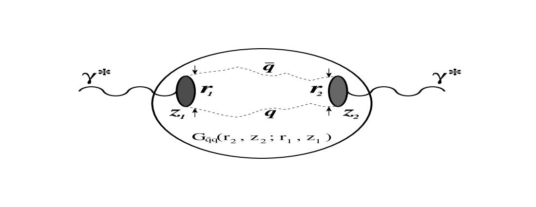
Figure 1: A cartoon for the shadowing term $\Delta\sigma_{tot}(x_{Bj},Q^{2})=\Delta\sigma_{tot}(\bar{q}q)$ in (2). Propagation of the $\bar{q}q$ pair through the nucleus is described by the Green function $G_{\bar{q}q}(\vec{r_{2}},z_{2};\vec{r_{1}},z_{1})$, which results from the summation over different paths of the $\bar{q}q$ pair.

The shadowing term $\Delta\sigma_{tot}(x_{Bj},Q^{2})=\Delta\sigma_{tot}(\bar{q}q)$ in (2) is illustrated in Fig. 1. At the point $z_{1}$ the initial photon diffractively produces the $\bar{q}q$ pair ($\gamma^{*}N\to\bar{q}qN$) with transverse separation $\vec{r_{1}}$. The $\bar{q}q$ pair then propagates through the nucleus along arbitrary curved trajectories, which are summed over, and arrives at the point $z_{2}$ with transverse separation $\vec{r_{2}}$. The initial and final separations are controlled by the LC wave function of the $\bar{q}q$ Fock component of the photon $\Psi_{\bar{q}q}(\vec{r},\alpha,Q^{2})$. During propagation through the nucleus the $\bar{q}q$ pair interacts with bound nucleons via the dipole cross section $\sigma_{\bar{q}q}(r,s)$, which depends on the local transverse separation $\vec{r}$. The Green function $G_{\bar{q}q}(\vec{r_{2}},z_{2};\vec{r_{1}},z_{1})$ describes the propagation of the $\bar{q}q$ pair from $z_{1}$ to $z_{2}$.

Describing the propagation of the $\bar{q}q$  pair in a  nuclear  medium, the  Green  function  $G_{\bar{q}q}(\vec{r_{2}},z_{2};\vec{r_{1}},z_{1})$ satisfies again the time-dependent two-dimensional Schrödinger equation (13). However, the potential in this case acquires in addition an imaginary part. This imaginary part of the LC potential $V_{\bar{q}q}(z_{2},\vec{r}_{2},\alpha)$ in Eq. (13) is responsible for the attenuation of the $\bar{q}q$ photon fluctuation in the medium, and has the following form

$$ImV_{\bar{q}q}(z_{2},\vec{r},\alpha)=-\frac{\sigma_{\bar{q}q}(\vec{r},s)}{2}\,\rho_{A}({b},z_{2})\,.$$ (34)

As was already mentioned above, the analytical solution of Eq. (13) is known only for the harmonic oscillator potential $V_{\bar{q}q}(r)\propto r^{2}$. Consequently, in order to keep such an analytical solution one should also use a quadratic approximation for the imaginary part of $V_{\bar{q}q}(z_{2},\vec{r}_{2},\alpha)$, i.e.

$$\sigma_{\bar{q}q}(r,s)=C(s)\,r^{2}\ ,$$ (35)

and uniform nuclear density

$$\rho_{A}(b,z)=\rho_{0}~{}\Theta(R_{A}^{2}-b^{2}-z^{2})\,.$$ (36)

In this case the solution of Eq. (13) has the same form as Eq. (16), except that one should replace $\omega\Longrightarrow\Omega$ and $a^{2}(\alpha)\Longrightarrow b(\alpha)$, where

$$\Omega=\frac{b(\alpha)}{\nu\alpha(1-\alpha)}=\frac{\sqrt{a^{4}(\alpha)-i\,\rho_{A}(b,z)\,\nu\,\alpha\,(1-\alpha)\,C(s)}}{\nu\,\alpha\,(1-\alpha)}\,.$$ (37)

The determination of the energy dependent factor $C(s)$ in Eq. (35) and the mean nuclear density $\rho_{0}$ in Eq. (36) can be realized by the procedure described in [17, 23, 18], and will be discussed below.

Investigating nuclear shadowing in DIS one can distinguish between two regimes, depending on the value of the coherence length:

(i) We start with the general case when there are no restrictions for $l_{c}$. If $l_{c}\sim R_{A}$ one has to take into account the variation of the transverse size $r$ during propagation of the $\bar{q}q$ pair through the nucleus, which is naturally included using a correct quantum-mechanical treatment based on the Green function formalism presented above. The overall total photoabsorption cross section on a nucleus is given as a sum over T and L polarizations, $\sigma^{\gamma^{*}A}=\sigma_{T}^{\gamma^{*}A}+\epsilon^{\prime}\,\sigma_{L}^{\gamma^{*}A}$, assuming that the photon polarization $\epsilon^{\prime}=1$. If one takes into account only the $\bar{q}q$ Fock component of the photon, the full expression after summation over all flavors, colors, helicities and spin states becomes [42]

$$\sigma^{\gamma^{*}A}(x_{Bj},Q^{2}) = A\,\sigma^{\gamma^{*}N}(x_{Bj},Q^{2})-\Delta\,\sigma(x_{Bj},Q^{2})$$

$$= A\,\int\,d^{2}r\,\int_{0}^{1}\,d\alpha\,\sigma_{\bar{q}q}(r,s)\,\Biggl{(}\Bigl{|}\Psi^{T}_{\bar{q}q}(\vec{r},\alpha,Q^{2})\Bigr{|}^{2}+\Bigl{|}\Psi^{L}_{\bar{q}q}(\vec{r},\alpha,Q^{2})\Bigr{|}^{2}\Biggr{)}$$

$$- \frac{N_{C}\,\alpha_{em}}{(2\pi)^{2}}\,\sum_{f=1}^{N_{f}}\,Z_{f}^{2}\,Re\,\int\,d^{2}b\,\int_{-\infty}^{\infty}\,dz_{1}\,\int_{z_{1}}^{\infty}\,dz_{2}\,\int_{0}^{1}\,d\alpha\,\int\,d^{2}r_{1}\,\int\,d^{2}r_{2}$$

$$\times\,\rho_{A}(b,z_{1})\,\rho_{A}(b,z_{2})\,\sigma_{\bar{q}q}(r_{2},s)\,\sigma_{\bar{q}q}(r_{1},s)$$

$$\times\,\Biggl{\{}\Bigl{[}\,\alpha^{2}+(1-\alpha)^{2}\,\Bigr{]}\,\epsilon^{2}\,\frac{\vec{r_{1}}\,\cdot\,\vec{r_{2}}}{r_{1}\,r_{2}}\,K_{1}(\epsilon\,r_{1})\,K_{1}(\epsilon\,r_{2})$$

$$\,\,\,\,\,\,\,\,\,\,\,\,\,\,\,+\,\Bigl{[}\,m_{f}^{2}+4\,Q^{2}\,\alpha^{2}\,(1-\alpha)^{2}\,\Bigr{]}\,K_{0}(\epsilon\,r_{1})\,K_{0}(\epsilon\,r_{2})\Biggr{\}}\,G_{\bar{q}q}(\vec{r_{2}},z_{2};\vec{r_{1}},z_{1})\,.$$

Here $\Bigl{|}\,\Psi^{T,L}_{\bar{q}q}(\vec{r},\alpha,Q^{2})\,\Bigr{|}^{2}$ are the absolute squares of the LC wave functions for the $\bar{q}q$ fluctuation of T and L polarized photons, summed over all flavors, and with the form given by Eqs. (27) and (28), respectively.

If one takes into account the nonperturbative interaction effects between $\bar{q}$ and $q$ of the virtual photon the expression for $\sigma^{\gamma^{*}A}(x_{Bj},Q^{2})$ Eq. (2) takes the following form:

$$\sigma^{\gamma^{*}A}_{npt}(x_{Bj},Q^{2}) = A\,\sigma^{\gamma^{*}N}_{npt}(x_{Bj},Q^{2})-\Delta\,\sigma_{npt}(x_{Bj},Q^{2})$$

$$= A\,\int\,d^{2}r\,\int_{0}^{1}\,d\alpha\,\sigma_{\bar{q}q}(r,s)\,\Biggl{(}\Bigl{|}\Psi^{T}_{npt}(\vec{r},\alpha,Q^{2})\Bigr{|}^{2}+\Bigl{|}\Psi^{L}_{npt}(\vec{r},\alpha,Q^{2})\Bigr{|}^{2}\Biggr{)}$$

$$- {N_{C}\,\alpha_{em}}\,\sum_{f=1}^{N_{f}}\,Z_{f}^{2}\,Re\,\int\,d^{2}b\,\int_{-\infty}^{\infty}\,dz_{1}\,\int_{z_{1}}^{\infty}\,dz_{2}\,\int_{0}^{1}\,d\alpha\,\int\,d^{2}r_{1}\,\int\,d^{2}r_{2}$$

$$\times\,\rho_{A}(b,z_{1})\,\rho_{A}(b,z_{2})\,\sigma_{\bar{q}q}(r_{2},s)\,\sigma_{\bar{q}q}(r_{1},s)$$

$$\times\,\Biggl{\{}\Bigl{[}\,\alpha^{2}+(1-\alpha)^{2}\,\Bigr{]}\,\vec{\Phi}_{1}(\epsilon\,,r_{1},\lambda)\cdot\vec{\Phi}_{1}(\epsilon\,,r_{2},\lambda)$$

$$\,\,\,\,\,\,\,\,\,\,\,\,\,+\,\Bigl{[}\,m_{f}^{2}+4\,Q^{2}\,\alpha^{2}\,(1-\alpha)^{2}\,\Bigr{]}\,\Phi_{0}(\epsilon\,,r_{1},\lambda)\,\Phi_{0}(\epsilon\,,r_{2},\lambda)\Biggr{\}}\,G_{\bar{q}q}(\vec{r_{2}},z_{2};\vec{r_{1}},z_{1})\,.$$

where $\Bigl{|}\,\Psi^{T,L}_{npt}(\vec{r},\alpha,Q^{2})\,\Bigr{|}^{2}$ are now given by Eqs. (30) and (31), respectively.

(ii) The CL is much larger than the mean nucleon spacing in a nucleus ($l_{c}\gg R_{A}$), which is the high energy limit. Correspondingly, the transverse separation $r$ between $\bar{q}$ and $q$ does not vary during propagation through the nucleus (Lorentz time dilation). In this case the eikonal formula for the total photoabsorption cross section on a nucleus can be obtained as a limiting case of the Green function formalism. Indeed, in the high energy limit $\nu\rightarrow\infty$, the kinetic term in Eq. (13) can be neglected and the Green function reads

$$G_{\bar{q}q}(b;\vec{r_{2}},z_{2};\vec{r_{1}},z_{1})|_{\nu\to\infty}=\delta(\vec{r_{2}}-\vec{r_{1}})\,\exp\Biggl{[}-\frac{1}{2}\,\sigma_{\bar{q}q}(r_{2},s)\,\int_{z_{1}}^{z_{2}}\,dz\,\rho_{A}(b,z)\Biggr{]}\,.$$ (40)

Including nonperturbative interaction effects between $\bar{q}$ and $q$, after substitution of the expression (40) into Eq. (2), one arrives at the following results:

$$\sigma^{\gamma^{*}A}_{npt}(x_{Bj},Q^{2}) = 2\,\int\,d^{2}b\,\int\,d^{2}r\,\int_{0}^{1}\,d\alpha\left\{1-\exp\,\Bigl{[}-\frac{1}{2}\,\sigma_{\bar{q}q}(r,s)\,T_{A}(b)\Bigr{]}\,\right\}$$

$$\times\,{2\,N_{C}\,\alpha_{em}}\,\sum_{f=1}^{N_{f}}\,Z_{f}^{2}\,\Biggl{\{}\Bigl{[}\,\alpha^{2}+(1-\alpha)^{2}\,\Bigr{]}\,\Bigl{|}\vec{\Phi}_{1}(\epsilon\,,r,\lambda)\Bigr{|}^{2}\,$$

$$\,\qquad\qquad\qquad\qquad+\,\Bigl{[}\,m_{f}^{2}+4\,Q^{2}\,\alpha^{2}\,(1-\alpha)^{2}\,\Bigr{]}\,\Phi_{0}^{2}(\epsilon\,,r,\lambda)\,\Biggr{\}}\,,$$

where

$$T_{A}(b)=\int_{-\infty}^{\infty}\,dz\,\rho_{A}(b,z)\,$$ (42)

is the nuclear thickness calculated with the realistic Wood-Saxon form of the nuclear density, with parameters taken from [43].

At the photon polarization parameter $\epsilon^{\prime}=1$ the structure function ratio $F_{2}^{A}/F_{2}^{N}$ is related to nuclear shadowing $R(A/N$ and can be expressed via a ratio of the total photoabsorption cross sections

$$\frac{F_{2}^{A}(x_{Bj},Q^{2})}{F_{2}^{N}(x_{Bj},Q^{2})}=A\,R(A/N)=\frac{\sigma_{T}^{\gamma^{*}A}(x_{Bj},Q^{2})+\sigma_{L}^{\gamma^{*}A}(x_{Bj},Q^{2})}{\sigma_{T}^{\gamma^{*}N}(x_{Bj},Q^{2})+\sigma_{L}^{\gamma^{*}N}(x_{Bj},Q^{2})}\,,$$ (43)

where the numerator on the right-hand side (r.h.s.) is given by Eq. (2), whereas the denominator can be expressed as the first term of Eq. (2) divided by the mass number $A$.

As we already mentioned above, an explicit analytical expression for the Green function $G_{\bar{q}q}(\vec{r_{2}},z_{2};\vec{r_{1}},z_{1})$ (16) can be found only for the quadratic form of the dipole cross section (35), and for uniform nuclear density function (36). It was shown in refs. [19, 23, 17, 18] that such an approximation gives results of reasonable accuracy, especially at small $x_{Bj}\mathrel{\hbox to0.0pt{\lower 4.0pt\hbox{\hskip 1.0pt$\sim$}\hss}\raise 1.0pt\hbox{$<$}}10^{-4}$ and for heavy nuclei. Nevertheless, it can be even more precise if one considers the fact that the expression (2) in the high energy limit can be easily calculated using realistic parametrizations of the dipole cross section (see Eq. (6) for the KST parametrization and ref. [32] for the GBW parametrization) and a realistic nuclear density function $\rho_{A}(b,z)$ [43]. Consequently, one needs to know the full Green function only in the transition region from non-shadowing ($x_{Bj}\sim 0.1$) to a fully developed shadowing given when coherence length $l_{c}\gg R_{A}$, which corresponds to $x_{Bj}\mathrel{\hbox to0.0pt{\lower 4.0pt\hbox{\hskip 1.0pt$\sim$}\hss}\raise 1.0pt\hbox{$<$}}10^{-4}$ depending on the value of $Q^{2}$. Therefore, the value of the energy dependent factor $C(s)$ in Eq. (35) can be determined by the procedure described in refs. [17, 23, 20]. According to this procedure, the factor $C(s)$ is adjusted by demanding that calculations employing the approximation (35) reproduce correctly the results for nuclear shadowing in DIS based on the realistic parametrizations of the dipole cross section Eq. (6) in the limit $l_{c}\gg R_{A}$, when the Green function takes the simple form (40). Consequently, the factor $C(s)$ is fixed by the relation

$$\frac{\int d^{2}\,b\,\int d^{2}\,r\,\Bigl{|}\Psi_{\bar{q}q}(\vec{r},\alpha,Q^{2})\Bigr{|}^{2}\,\left\{1-\exp\,\Bigl{[}-\frac{1}{2}\,C(s)\,r^{2}\,T_{A}(b)\Bigr{]}\,\right\}}{\int d^{2}\,r\,\Bigl{|}\Psi_{\bar{q}q}(\vec{r},\alpha,Q^{2})\Bigr{|}^{2}\,C(s)\,r^{2}}$$

$$=\frac{\int d^{2}\,b\,\int d^{2}\,r\,\Bigl{|}\Psi_{\bar{q}q}(\vec{r},\alpha,Q^{2})\Bigr{|}^{2}\,\left\{1-\exp\,\Bigl{[}-\frac{1}{2}\,\sigma_{\bar{q}q}(r,s)\,T_{A}(b)\Bigr{]}\,\right\}}{\int d^{2}\,r\,\Bigl{|}\Psi_{\bar{q}q}(\vec{r},\alpha,Q^{2})\Bigr{|}^{2}\,\sigma_{\bar{q}q}(r,s)}\,.$$ (44)

Correspondingly, the value $\rho_{0}$ of the uniform nuclear density (36) is fixed in an analogous way using the following relation

$$\int\,d^{2}\,b\,\Biggl{[}1-exp\,\Biggl{(}-\sigma_{0}\,\rho_{0}\,\sqrt{R_{A}^{2}-b^{2}}\,\Biggr{)}\,\Biggr{]}=\int\,d^{2}\,b\,\Biggl{[}1-exp\,\Biggl{(}-\frac{1}{2}\,\sigma_{0}\,T_{A}(b)\,\Biggr{)}\,\Biggr{]}\,,$$ (45)

where the value of $\rho_{0}$ was found to be practically independent of the cross section $\sigma_{0}$, when this changed from 1 to 50 mb [17, 23]. Such a procedure for the determination of the factors $C(s)$ and $\rho_{0}$ was applied also in refs. [20, 21], in the case of incoherent and coherent production of vector mesons off nuclei.

In order to remove the above mentioned uncertainties the evolution equation for the Green function was solved numerically for the first time in ref. [18]. Such an exact solution can be performed for arbitrary parametrization of the dipole cross section and for realistic nuclear density functions, although the nice analytical form for the Green function is lost in this case.

In the process of numerical solution of the Schrödinger equation (13) for the Green function $G_{\bar{q}q}(\vec{r_{2}},z_{2};\vec{r_{1}},z_{1})$ with the initial condition (14), it is much more convenient to use the following substitutions [18]

$$g_{0}(\vec{r_{2}},z_{2};z_{1},\lambda)=\int\,d^{2}r_{1}\,\Phi_{0}(\epsilon\,,r_{1},\lambda)\,\sigma_{\bar{q}q}(r_{1},s)\,G_{\bar{q}q}(\vec{r_{2}},z_{2};\vec{r_{1}},z_{1})\,,$$ (46)

and

$$\frac{\vec{r_{2}}}{r_{2}}\,g_{1}(\vec{r_{2}},z_{2};z_{1},\lambda)=\int\,d^{2}r_{1}\,\vec{\Phi}_{1}(\epsilon\,,r_{1},\lambda)\,\sigma_{\bar{q}q}(r_{1},s)\,G_{\bar{q}q}(\vec{r_{2}},z_{2};\vec{r_{1}},z_{1})\,.$$ (47)

After some algebra with Eq. (13) these new functions  $g_{0}(\vec{r_{2}},z_{2};z_{1},\lambda)$ and  $g_{1}(\vec{r_{2}},z_{2};z_{1},\lambda)$ can be shown to satisfy the following evolution equations

$$i\frac{d}{dz_{2}}\,g_{0}(\vec{r_{2}},z_{2};z_{1},\lambda)=\left\{\frac{1}{2\,\mu_{\bar{q}q}}\left[\epsilon^{2}-\frac{\partial^{2}}{\partial\,r_{2}^{2}}-\frac{1}{r_{2}}\,\frac{\partial}{\partial\,r_{2}}\right]+V_{\bar{q}q}(z_{2},\vec{r}_{2},\alpha)\right\}g_{0}(\vec{r_{2}},z_{2};z_{1},\lambda)\$$ (48)

and

$$i\frac{d}{dz_{2}}\,g_{1}(\vec{r_{2}},z_{2};z_{1},\lambda)=\left\{\frac{1}{2\,\mu_{\bar{q}q}}\left[\epsilon^{2}-\frac{\partial^{2}}{\partial\,r_{2}^{2}}-\frac{1}{r_{2}}\,\frac{\partial}{\partial\,r_{2}}+\frac{1}{r_{2}^{2}}\right]+V_{\bar{q}q}(z_{2},\vec{r}_{2},\alpha)\right\}g_{1}(\vec{r_{2}},z_{2};z_{1},\lambda)\ ,$$ (49)

with the boundary conditions

$$g_{0}(\vec{r_{2}},z_{2};z_{1},\lambda)|_{z_{2}=z_{1}}=\Phi_{0}(\epsilon\,,r_{2},\lambda)\,\sigma_{\bar{q}q}(r_{2},s)$$ (50)

and

$$g_{1}(\vec{r_{2}},z_{2};z_{1},\lambda)|_{z_{2}=z_{1}}=\tilde{\Phi}_{1}(\epsilon\,,r_{2},\lambda)\,\sigma_{\bar{q}q}(r_{2},s)\,,$$ (51)

where $\tilde{\Phi}_{1}(\epsilon\,,r,\lambda)$ is connected with $\vec{\Phi}_{1}(\epsilon\,,r,\lambda)$ by the following relation:

$$\vec{\Phi}_{1}(\epsilon\,,r,\lambda)=\frac{\vec{r}}{r}\tilde{\Phi}_{1}(\epsilon\,,r,\lambda)\,.$$ (52)

In Eqs. (48) and (49) the quantity

$$\mu_{\bar{q}q}=\nu\,\alpha\,(1-\alpha)$$ (53)

plays the role of the reduced mass of the $\bar{q}q$ pair.

Now the expression (2) for total photoabsorption cross section on a nucleus reads

$$\sigma^{\gamma^{*}A}_{npt}(x_{Bj},Q^{2}) = A\,\sigma^{\gamma^{*}N}_{npt}(x_{Bj},Q^{2})-\Delta\,\sigma(x_{Bj},Q^{2})$$

$$= A\,\int\,d^{2}r\,\int_{0}^{1}\,d\alpha\,\sigma_{\bar{q}q}(r,s)\,\Biggl{(}\Bigl{|}\Psi^{T}_{npt}(\vec{r},\alpha,Q^{2})\Bigr{|}^{2}+\Bigl{|}\Psi^{L}_{npt}(\vec{r},\alpha,Q^{2})\Bigr{|}^{2}\Biggr{)}$$

$$- {3\,\alpha_{em}}\,\sum_{f=1}^{N_{f}}\,Z_{f}^{2}\,\,Re\,\int\,d^{2}b\,\int_{-\infty}^{\infty}\,dz_{1}\,\int_{z_{1}}^{\infty}\,dz_{2}\,\int_{0}^{1}\,d\alpha\,\int\,d^{2}r_{2}$$

$$\times\,\rho_{A}(b,z_{1})\,\rho_{A}(b,z_{2})\,\sigma_{\bar{q}q}(r_{2},s)\,$$

$$\times\,\Biggl{\{}\Bigl{[}\,\alpha^{2}+(1-\alpha)^{2}\,\Bigr{]}\,\tilde{\Phi}_{1}(\epsilon\,,r_{2},\lambda)\,g_{1}(\vec{r_{2}},z_{2};z_{1},\lambda)$$

$$\,\,\,\,\,\,\,\,\,\,\,\,\,\,\,+\,\Bigl{[}\,m_{f}^{2}+4\,Q^{2}\,\alpha^{2}\,(1-\alpha)^{2}\,\Bigr{]}\,\Phi_{0}(\epsilon\,,r_{2},\lambda)\,g_{0}(\vec{r_{2}},z_{2};z_{1},\lambda)\Biggr{\}}\,.$$

Notice that this equation explicitly includes nonperturbative interaction effects between $\bar{q}$ and $q$. Details of the algorithm for the numerical solution of Eqs. (48) and (49) can be found in ref. [18].

Finally we would like to emphasize that the $\bar{q}q$ Fock component of the photon represents the highest twist shadowing correction [17], and vanishes at large quark masses as $1/m_{f}^{2}$. This does not happen for higher Fock states containing gluons, which lead to GS. Therefore GS represents the leading twist shadowing correction [24, 44]. Moreover, a steep energy dependence of the dipole cross section $\sigma_{\bar{q}q}(r,s)$ (see Eq. (6)) especially at smaller dipole sizes $r$ causes a steep energy rise of both corrections.

3 Gluon shadowing

In the LC Green function approach [19, 17, 20, 21, 18] the physical photon $|\gamma^{*}\rangle$ is decomposed into different Fock states, namely, the bare photon $|\gamma^{*}\rangle_{0}$, plus $|\bar{q}q\rangle$, $|\bar{q}qG\rangle$, etc. As we mentioned above the higher Fock states containing gluons describe the energy dependence of the photoabsorption cross section on a nucleon, and also lead to GS in the nuclear case. However, these fluctuations are heavier and have a shorter coherence time (lifetime) than the lowest $|\bar{q}q\rangle$ state, and therefore at small and medium energies only the $|\bar{q}q\rangle$ fluctuations of the photon matter. Consequently, GS, which is related to the higher Fock states, will dominate at higher energies, i.e. at small values of $x_{Bj}\mathrel{\hbox to0.0pt{\lower 4.0pt\hbox{\hskip 1.0pt$\sim$}\hss}\raise 1.0pt\hbox{$<$}}0.01$. Since we will study the shadowing region of $x_{Bj}\mathrel{\hbox to0.0pt{\lower 4.0pt\hbox{\hskip 1.0pt$\sim$}\hss}\raise 1.0pt\hbox{$<$}}0.01$ and the available experimental data reach values of $x_{Bj}$ down to $\sim 10^{-4}$, we will include GS in our calculations and show that it is not a negligible effect. Besides, no data for gluon shadowing are available and one has to rely on calculations.

In the previous Section 2 we discussed the nuclear shadowing for the $|\bar{q}q\rangle$ Fock component of the photon. It is dominated by the transverse photon polarizations, because the corresponding photoabsorption cross section is scanned at larger dipole sizes than for the longitudinal photon polarization. The transverse $\bar{q}q$ separation is controlled by the distribution amplitude Eq. (8), with the mean value given by Eq. (12). Contributions of large size dipoles come from the asymmetric $\bar{q}q$ fluctuations of the virtual photon, when the quark and antiquark in the photon carry a very large ($\alpha\to 1$) and a very small fraction ($\alpha\to 0$) of the photon momentum, and vice versa. The LC wave function for longitudinal photons (28) contains a term $\alpha^{2}\,(1-\alpha)^{2}$, which makes considerably smaller the contribution from asymmetric $\bar{q}q$ configurations than for transversal photons (see Eq. (27)). Consequently, in contrast to transverse photons, all $\bar{q}q$ dipoles from longitudinal photons have a size squared $\propto 1/Q^{2}$ and the double-scattering term vanishes as $\propto 1/Q^{4}$. The leading-twist contribution for the shadowing of longitudinal photons arises from the $|\bar{q}qG\rangle$ Fock component of the photon because the gluon can propagate relatively far from the $\bar{q}q$ pair, although the $\bar{q}$-$q$ separation is of the order $1/Q^{2}$. After radiation of the gluon the pair is in an octet state, and consequently the $|\bar{q}qG\rangle$ state represents a $GG$ dipole. Then the corresponding correction to the longitudinal cross section is just gluon shadowing.

The phenomenon of GS, just as for the case of nuclear shadowing discussed in the Introduction, can be treated differently depending on the reference frame. In the infinite momentum frame this phenomenon looks similar to gluon-gluon fusion, corresponding to a nonlinear term in the evolution equation [45]. This effect should lead to a suppression of the small-$x_{Bj}$ gluons also in a nucleon, and lead to a precocious onset of the saturation effects for heavy nuclei. Within a parton model interpretation, in the infinite momentum frame of the nucleus the gluon clouds of nucleons which have the same impact parameter overlap at small $x_{Bj}$ in the longitudinal direction. This allows gluons originated from different nucleons to fuse, leading to a gluon density which is not proportional to the density of nucleons any more. This is gluon shadowing.

The same phenomenon looks quite different in the rest frame of the nucleus. It corresponds to the process of gluon radiation and shadowing corrections, related to multiple interactions of the radiated gluons in the nuclear medium [28]. This is a coherence phenomenon known as the Landau-Pomeranchuk effect, namely the suppression of bremsstrahlung by interference of radiation from different scattering centers, demanding a sufficiently long coherence time of radiation, a condition equivalent to a small Bjorken $x_{Bj}$ in the parton model.

Although these two different interpretations are not Lorentz invariant, they represent the same phenomenon, related to the Lorentz invariant Reggeon graphs. It was already discussed in detail in refs. [20, 46] that the double-scattering correction to the cross section of gluon radiation can be expressed in Regge theory via the triple-Pomeron diagram. It is interpreted as a fusion of two Pomerons originated from different nucleons, 2$\,{\bf I\!P}\rightarrow{\bf I\!P}$, which leads to a reduction of the nuclear gluon density $G_{A}$.

Notice that in the hadronic representation such a suppression of the parton density corresponds to Gribov’s inelastic shadowing [25], which is related to the single diffraction cross section. In particular, GS corresponds to the triple-Pomeron term in the diffractive dissociation cross section, which enters the calculations of inelastic corrections.

There are still very few numerical evaluations of gluon shadowing in the literature, all of them done in the rest frame of the nucleus, using the idea from ref. [28]. As was discussed above gluon shadowing can be identified as the shadowing correction to the longitudinal cross section coming from the $GG$ dipole representing the $|\bar{q}qG\rangle$ Fock component of the photon. An important point for the evaluation of GS is knowing about the transverse size of this $GG$ dipole. This size has been extracted in ref. [24] from data for diffractive excitation of the incident hadrons to the states of large mass, the so called triple-Pomeron region. The corresponding diffraction cross section ($\propto r^{4}$) is a more sensitive probe of the mean transverse separation than the total cross section ($\propto r^{2}$). Consequently, it was found in ref. [24] that the mean dipole size of the $GG$ system (radius of propagation of the LC gluons) is rather small , $r_{0}\approx 0.3\,\,\mbox{fm}$ [47]. Such a small quark-gluon fluctuation represents the only known way how to resolve the long-standing problem of the small size of the triple-Pomeron coupling.

To incorporate the smallness of the size of quark-gluon fluctuations into the LC dipole approach, a nonperturbative LC potential describing the quark-gluon interaction was introduced into the Schrödinger equation for the LC Green function describing the propagation of a quark-gluon system. The strength of the potential was fixed by data on high mass ($M_{X}^{2}$) diffraction $pp\to pX$ [24]. This approach allows to extend the methods of pQCD to the region of small $Q^{2}$. Since a new semihard scale $1/r_{0}\sim 0.65\,\,\mbox{GeV}$ is introduced, one should not expect a substantial variation of gluon shadowing at $Q^{2}\mathrel{\hbox to0.0pt{\lower 4.0pt\hbox{\hskip 1.0pt$\sim$}\hss}\raise 1.0pt\hbox{$<$}}4/r_{0}^{2}$. Indeed, the calculations performed in [24] for $Q^{2}=0$ and $4\,\,\mbox{GeV}^{2}$, using different techniques, led to about the same gluon shadowing. At higher $Q^{2}$ shadowing slowly (logarithmically) decreases, in accordance with the expectations based on the evolution equation [4], which clearly demonstrates that GS is a leading-twist effect.

In this paper we repeated the calculations [24] of the ratio of the gluon densities in nuclei and nucleon,

$$R_{G}(x_{Bj},Q^{2})=\frac{G_{A}(x_{Bj},Q^{2})}{A\,G_{N}(x_{Bj},Q^{2})}\approx 1-\frac{\Delta\sigma_{tot}(\bar{q}qG)}{\sigma_{tot}^{\gamma^{*}A}}\ ,$$ (55)

where $\Delta\sigma_{tot}(\bar{q}qG)$ is the inelastic correction to the total cross section $\sigma_{tot}^{\gamma^{*}A}$, related to the creation of a $|\bar{q}qG\rangle$ intermediate Fock state,

$$\Delta\sigma_{tot}(\bar{q}qG)={\rm Re}\int\limits_{-\infty}^{\infty}dz_{2}\int\limits_{-\infty}^{z_{2}}dz_{1}\,\rho_{A}(b,z_{1})\,\rho_{A}(b,z_{2})\int d^{2}x_{2}\,d^{2}y_{2}\,d^{2}x_{1}\,d^{2}y_{1}\int d\alpha_{q}\,\frac{d\,\alpha_{G}}{\alpha_{G}}$$ (56)

$$\times F^{\dagger}_{\gamma^{*}\to\bar{q}qG}(\vec{x}_{2},\vec{y}_{2},\alpha_{q},\alpha_{G})\ G_{\bar{q}qG}(\vec{x}_{2},\vec{y}_{2},z_{2};\vec{x}_{1},\vec{y}_{1},z_{1})\ F_{\gamma^{*}\to\bar{q}qG}(\vec{x}_{1},\vec{y}_{1},\alpha_{q},\alpha_{G})\ .$$

Here $\vec{x}$ and $\vec{y}$ are the transverse distances from the gluon to the quark and antiquark, respectively, $\alpha_{q}$ is the fraction of the LC momentum of the $\bar{q}q$ carried by the quark, and $\alpha_{G}$ is the fraction of the photon momentum carried by the gluon. $F_{\gamma^{*}\to\bar{q}qG}$ is the amplitude of diffractive $\bar{q}qG$ production in a $\gamma^{*}N$ interaction [24], and it is given by

$$F_{\gamma^{*}\to\bar{q}qG}(\vec{x},\vec{y},\alpha_{q},\alpha_{G}) = {9\over 8}\,\Psi_{\bar{q}q}(\alpha_{q},\vec{x}-\vec{y})\,\left[\Psi_{qG}\left(\frac{\alpha_{G}}{\alpha_{q}},\vec{x}\right)-\Psi_{\bar{q}G}\left(\frac{\alpha_{G}}{1-\alpha_{q}},\vec{y}\right)\,\right]$$ (57)

$$\times \biggl{[}\sigma_{\bar{q}q}(x)+\sigma_{\bar{q}q}(y)-\sigma_{\bar{q}q}(\vec{x}-\vec{y})\biggr{]}\ ,$$

where $\Psi_{\bar{q}q}$ and $\Psi_{\bar{q}G}$ are the LC distribution functions of the $\bar{q}q$ fluctuations of a photon and $qG$ fluctuations of a quark, respectively.

In the above equation $G_{\bar{q}qG}(\vec{x}_{2},\vec{y}_{2},z_{2};\vec{x}_{1},\vec{y}_{1},z_{1})$ is the LC Green function which describes the propagation of the $\bar{q}qG$ system from the initial state with longitudinal and transverse coordinates $z_{1}$ and $\vec{x}_{1},\vec{y}_{1}$, respectively, to the final coordinates $(z_{2},\vec{x}_{2},\vec{y}_{2})$. For the calculation of gluon shadowing one should suppress the intrinsic $\bar{q}q$ separation, i.e. assume $\vec{x}=\vec{y}$. In this case the Green function simplifies, and effectively describes the propagation of a gluon-gluon dipole through a medium.

An important finding of ref. [24] is the presence of a strong nonperturbative interaction which squeezes the gluon-gluon wave packet and substantially diminishes gluon shadowing. The smallness of the gluon-gluon transverse separation is not a model assumption, but is dictated by data for hadronic diffraction into large masses (triple-Pomeron regime), which is controlled by diffractive gluon radiation.

Figure 2: The ratio of the nucleus-to-nucleon gluon densities as function of the thickness of the nucleus, $L=T(b)/\rho_{0}$, at $Q^{2}=4\,\,\mbox{GeV}^{2}$ and different fixed values of $x_{Bj}$. Figure is taken from ref. [20].

Further calculational details can be found in [24]. In our case we calculated the gluon shadowing only for the lowest Fock component containing just one LC gluon. In terms of the parton model it reproduces the effects of fusion of many gluons to one gluon (in terms of Regge approach it corresponds to the $n{\bf I\!P}\to{\bf I\!P}$ vertex). Inclusion of higher multigluon Fock components is still a challenge. However, their effect can be essentially taken into account by the eikonalization of the calculated $R_{G}(x_{Bj},Q^{2})$, as argued in [48]. In other words, the dipole cross section, which is proportional to the gluon density at small separations, should be renormalized everywhere, in the form

$$\sigma_{\bar{q}q}\Rightarrow R_{G}\,\sigma_{\bar{q}q}\ .$$ (58)

Such a procedure makes the nuclear medium more transparent. This could be expected since Gribov’s inelastic shadowing is known to suppress the total hadron-nucleus cross sections, i.e. to make nuclei more transparent [29, 49].

As an illustration of not very strong onset of GS, here we present $R_{G}(x_{Bj},Q^{2})$, Eq. (55), for different nuclear thicknesses $T_{A}(b)$. Using an approximation of constant nuclear density (see Eq. (36)), $T_{A}(b)=\rho_{0}\,L$, where $L=2\,\sqrt{R_{A}^{2}-b^{2}}$, the ratio $R_{G}(x_{Bj},Q^{2})$ is also implicitly a function of $L$. An example for the calculated $L$-dependence of $R_{G}(x_{Bj},Q^{2})$ at $Q^{2}=4\,\,\mbox{GeV}^{2}$ is depicted in Fig. 2 for different values of $x_{Bj}$.

One can expect intuitively from Eq. (58) that GS should always diminish the nuclear cross sections of various processes in nuclear targets, and that the onset of GS is stronger for heavier nuclei. However, this is not so for incoherent electroproduction of vector mesons, analyzed in ref. [20]. The specific structure of the expression for the nuclear production cross section causes that the cross section of incoherent electroproduction of vector mesons is rather insensitive to GS. Furthermore, the effect of GS is stronger for light than for heavy nuclear targets, in contradiction with the standard intuition. Moreover, for heavy nuclei the effect GS can lead even to a counterintuitive enhancement (antishadowing), as was analyzed in ref. [20]. For the case of coherent vector meson production $\gamma^{*}A\to VA$ [20], GS was shown to be a much stronger effect in comparison with incoherent production, which confirms the expected reduction of the nuclear production cross section.

Similarly, it was analyzed in ref. [46] that multiple scattering of higher Fock states containing gluons leads to an additional suppression of the Drell-Yan cross section. In the present paper we will demonstrate that gluon shadowing also suppresses the total photoabsorption cross section on a nucleus $\sigma_{tot}^{\gamma^{*}A}(x_{Bj},Q^{2})$. Here we expect quite a strong effect of GS in the shadowing region of small $x_{Bj}\mathrel{\hbox to0.0pt{\lower 4.0pt\hbox{\hskip 1.0pt$\sim$}\hss}\raise 1.0pt\hbox{$<$}}(0.01\div 0.001)$, in the kinematic range of available data corresponding to small and medium values of $Q^{2}\sim$ a few GeV².

4 Numerical results

As we mentioned above the main goal of this paper is to compare for the first time available experimental data with realistic predictions for nuclear shadowing in DIS, based on exact numerical solutions of the evolution equation for the Green function. Such a comparison is performed for the shadowing region of small $x_{Bj}\mathrel{\hbox to0.0pt{\lower 4.0pt\hbox{\hskip 1.0pt$\sim$}\hss}\raise 1.0pt\hbox{$<$}}0.01$. As was discussed in the previous section one should take into account also a contribution of gluon shadowing, which increases the overall nuclear suppression. The effect of GS was already calculated in ref. [50], but only for the $F_{2}^{C}/F_{2}^{D}$ ratio of structure functions. Although the quark shadowing was compute approximately via longitudinal form factor of the nucleus and assuming only the leading shadowing term, it was shown that GS is a rather large effect at $x_{Bj}\sim 10^{-4}$. In the present paper we will also show that GS is not a negligible effect, and can in principle be detected by the data on the total photoabsorption nuclear cross section in future experiments.

The predictions for nuclear shadowing based on an exact numerical solution of the evolution equation was compared in ref. [18] with approximate results obtained using the harmonic oscillatory form of the Green function (16). Quite a large discrepancy was found, in the range of $x_{Bj}\mathrel{\hbox to0.0pt{\lower 4.0pt\hbox{\hskip 1.0pt$\sim$}\hss}\raise 1.0pt\hbox{$>$}}0.001$, where the variation of the transverse size of the $\bar{q}q$ pair during propagation through the nucleus becomes important. Such a variation is naturally included in the Green function formalism and consequently the exact shape of the Green function is extremely important.

We use an algorithm for the numerical solution of the Schrödinger equation for the Green function, as developed and described in ref. [18]. This gives the possibility of calculating nuclear shadowing for arbitrary LC potentials $V_{\bar{q}q}(z,\vec{r},\alpha)$ and nuclear density functions. Because the available data from the E665 [51, 52] and NMC [53, 54] collaborations cover the region of small and medium values of $Q^{2}\mathrel{\hbox to0.0pt{\lower 4.0pt\hbox{\hskip 1.0pt$\sim$}\hss}\raise 1.0pt\hbox{$<$}}4\,\,\mbox{GeV}^{2}$, we prefer the KST parametrization of the dipole cross section (6), which is valid down to the limit of real photoproduction. On the contrary, the second GBW parametrization [32] of the dipole cross section cannot be applied in the nonperturbative region and therefore we do not use it in our calculations.

In the process of exact numerical solutions of the evolution equation for the Green function, the imaginary part of the LC potential (34) contains the corresponding KST dipole cross section as well. The nuclear density function $\rho_{A}({b},z)$ was taken in the realistic Wood-Saxon form, with parameters taken from ref. [43]. The nonperturbative interaction effects between $\bar{q}$ and $q$ are included explicitly via the real part of the LC potential of the form (15), which is supported also by the fact that the data from E665 and NMC collaborations correspond to very small values of $Q^{2}\mathrel{\hbox to0.0pt{\lower 4.0pt\hbox{\hskip 1.0pt$\sim$}\hss}\raise 1.0pt\hbox{$<$}}1\,\,\mbox{GeV}^{2}$ in the region of small $x_{Bj}\mathrel{\hbox to0.0pt{\lower 4.0pt\hbox{\hskip 1.0pt$\sim$}\hss}\raise 1.0pt\hbox{$<$}}0.004$.

Figure 3: Nuclear shadowing for lead. Calculations correspond to exact numerical solution of the evolution equation for the Green function using the KST [24] parametrization of the dipole cross section and a realistic nuclear density function of the Woods-Saxon form [43]. The thick and thin solid curves represent the predictions calculated with and without contribution of gluon shadowing, respectively. The dotted lines are calculated using a constant nuclear density function (36) and the quadratic form of the dipole cross section, $\sigma(r,s)=C(s)\,r^{2}$, where the energy dependent factor C(s) is determined by Eq. (44). The dashed curves are calculated for the same quadratic form of the dipole cross section, but for the realistic nuclear density function ([43])

We included also the effects of gluon shadowing for the lowest Fock component containing just one LC gluon. Although the inclusion of higher Fock components with more gluons is complicated, their effect was essentially taken into account by eikonalization of the calculated $R_{G}(x_{Bj},Q^{2})$ [48], i.e using the renormalization (58).

Nuclear shadowing effects were studied via the $x_{Bj}$- behavior of the ratio of proton structure functions (43) divided by the mass number $A$. First we present nuclear shadowing for a lead target in Fig. 3 at different fixed values of $Q^{2}$. The thick and thin solid curves represent the predictions obtained with and without the contribution of gluon shadowing, respectively.

Figure 4: Comparison of the model with experimental data from the E665 [51, 52] and NMC [53, 54] collaborations. Calculations correspond to the exact numerical solution of the evolution equation for the Green function using KST [24] parametrization of the dipole cross section and a realistic nuclear density function of the Woods-Saxon form [43]. The solid and dashed curves are calculated with and without the contribution of gluon shadowing, respectively.

One can see that the onset of GS happens at smaller $x_{Bj}$ than the quark shadowing, which is supported by the fact that higher Fock fluctuations containing gluons are in general heavier than $\bar{q}q$ and have a shorter coherence length. Fig. 3 demonstrates quite a strong effect of GS in the range of $x_{Bj}\in(0.01,0.0001)$ where the most of available data exist. This is a result of the suppression of the dipole cross section by the renormalization (58), which can result only in a reduction of the total photoabsorption cross section on a nuclear target. Besides the effect of GS is stronger at smaller $Q^{2}$ because corresponding Fock fluctuations of the photon have a larger transverse size.

In Fig. 3 we also present, for comparison and by the dotted lines, the approximate predictions for nuclear shadowing in DIS using constant nuclear density (36) and the quadratic form of the dipole cross section, $\sigma(r,s)=C(s)\,r^{2}$. The energy dependent factor C(s) is determined by Eq. (44), and the uniform nuclear density is fixed by the condition (45). One can see that these approximate predictions overestimate the values of nuclear shadowing obtained by means of an exact numerical solution of the evolution equation for the Green function. The difference from the exact calculation (thin solid lines) is not large and rises towards small values of $Q^{2}$. The reason is that the quadratic approximation of the dipole cross section cannot be applied exactly at large dipole sizes. Since the available data from the E665 [51, 52] and NMC [53, 54] collaborations at smallest values of $x_{Bj}$ correspond also to small $Q^{2}\ll 1\,\,\mbox{GeV}^{2}$, one can expect a larger difference between the exact and approximate results in comparison with what is shown in Fig. 3 at $Q^{2}=2\,\,\mbox{GeV}^{2}$. Keeping the quadratic form of the dipole cross section, but using the realistic nuclear density [43], one can obtain the results depicted in Fig. 3 by the dashed lines. It brings a better agreement with the exact calculations.

At low $x_{Bj}\mathrel{\hbox to0.0pt{\lower 4.0pt\hbox{\hskip 1.0pt$\sim$}\hss}\raise 1.0pt\hbox{$<$}}10^{-4}$ one should expect a saturation of nuclear shadowing at the level given by Eq. (2). This is realized only for the dipole cross section, without energy dependence, i.e. for example for parametrization (35) of the dipole cross section with constant factor $C(s)\approx 3$ [19]. However, this is not so for the realistic KST parametrization Eq. (6), where the saturation level is not fixed exactly due to energy (Bjorken $x_{Bj}$-) dependence of the dipole cross section $\sigma_{\bar{q}q}(r,s)$.

Figure 5: Model predictions for nuclear shadowing for a broad $x_{Bj}$-region down to $10^{-7}$ corresponding to LHC kinematical range at three different values of $Q^{2}=2$, $6$ and $18\,\,\mbox{GeV}^{2}$. Calculations of the nuclear shadowing for the $\bar{q}q$ Fock component of the photon correspond to the exact numerical solution of the evolution equation for the Green function using KST [24] parametrization of the dipole cross section and a realistic nuclear density function of the Woods-Saxon form [43]. The solid and dashed curves are calculated with and without the contribution of gluon shadowing, respectively.

In Fig. 4 we present a comparison of the model predictions with experimental data at small $x_{Bj}$, from the E665 [51, 52] and NMC [53, 54] collaborations. One can see a quite reasonable agreement with experimental data, in spite of the absence of any free parameters in the model. Several comments are in order: first, if GS is not taken into account, for the C/D and Ca/D ratios the nuclear shadowing looks overestimated in comparison with the E665 data for $x_{Bj}\sim 0.01$, while it looks in a good agreement for C/D, and a little bit underestimated for Ca/D in comparison with the NMC data. This is affected by the known incompatibility of the results from both experiments for the ratios over D. Second, as was discussed in the previous section, the effect of GS produces an additional nuclear shadowing which rises with mass number $A$. Consequently, it leads to a small overestimation of the nuclear shadowing for the C/D and Ca/D ratios in comparison with the E665 data, but it seems to be a in good agreement with the NMC data.

Figure 6: The same as Fig.5 but with GBW [32] parametrization of the dipole cross section.

For heavy nuclear targets there is only E665 data for the ratios Xe/D and Pb/D. Fig. 4 shows a reasonable good description of these data, even if the effect of GS is taken into account. The difference between the solid and dashed lines in Fig. 4 represents quite a large effect of GS, which was neglected up to the present time in calculations of nuclear shadowing in DIS [19, 17, 23] assuming that it would be a very small effect in the kinematic range covered by the available experimental data. On the contrary, looking at Fig. 4 one can see that the effect of GS as an additional nuclear shadowing cannot be neglected and should be included in calculations already in the region of $x_{Bj}\mathrel{\hbox to0.0pt{\lower 4.0pt\hbox{\hskip 1.0pt$\sim$}\hss}\raise 1.0pt\hbox{$<$}}0.01\div 0.001$. Very large error bars especially at small $x_{Bj}\sim 10^{-4}$ do not allow to investigate separately the effect of GS, and therefore more exact new data on nuclear shadowing in DIS at small $x_{Bj}$ are very important for further exploratory studies of the nuclear modification of structure functions and also for gluon shadowing.

For completeness we present also in Figs. 5 and 6 predictions for nuclear shadowing down to very small $x_{Bj}=10^{-7}$ accesible by experiments at LHC using two different realistic parametrizations of the dipole cross section, KST [24] and GBW [32]. Again, one can see quite large effect of GS as a difference between the solid and dashed lines.

Here, we would like to emphasize that at $x_{Bj}\mathrel{\hbox to0.0pt{\lower 4.0pt\hbox{\hskip 1.0pt$\sim$}\hss}\raise 1.0pt\hbox{$<$}}10^{-4}$ transverse size separations of the photon fluctuations are “frozen” during propagation through nuclear medium and one can use the simplified expressions, Eq. (40) and (2) for calculation of nuclear shadowing.

Figure 7: Comparison of the model results for the ratio Pb/nucleon obtained without (upper thick solid line) and with (lower thick solid line) gluon shadowing, with other models, versus $x_{Bj}$, at fixed $Q^{2}=3\,\,\mbox{GeV}^{2}$. Bartels are the results from [58], Frankfurt from [55] ($Q^{2}=4\,\,\mbox{GeV}^{2}$), and ACKLS from [56].

Finally, we present in Fig. 7 a comparison of the nuclear shadowing calculated using our model with the results of other models, for $Q^{2}=3\,\,\mbox{GeV}^{2}$ (except the results of ref. [55], which are at $Q^{2}=4\,\,\mbox{GeV}^{2}$). Notice that the difference between models rises towards small values of $x_{Bj}$, as a result of the different treatment of various nuclear effects, and absence of relevant experimental information at such small $x_{Bj}$. At $x_{Bj}=10^{-5}$ we predict quite a large effect of GS (compare upper and lower thick solid lines).

In ref. [56] nuclear structure functions were studied using relation with diffraction on nucleons known as Gribov inelastic corrections. The results of these calculations are depicted in Fig. 7 by dotted curves.

The model presented in [55] employs again a parametrization of hard diffraction at the scale $Q_{0}^{2}$, which gives nuclear shadowing in terms of Gribov’s corrections similar to ref. [56]. Then the nuclear suppression calculated at $Q^{2}_{0}$ is used as initial condition for Dokshitzer-Gribov-Lipatov-Altareli-Parisi (DGLAP) [57] evolution. This results are presented in Fig. 7 by dashed curves.

The model based on a numerical solution of the non-linear equation for small-$x_{Bj}$ evolution in nuclei was employed in [58]. The result is shown in Fig. 7 by thin solid curve.

At very small $x_{Bj}$ our model predictions, including the effect of GS, roughly agrees with those of [56], but lie below the results of other models. If the effect of GS is not taken into account the situation is substantially different and the corresponding curve (see upper thick solid line) lies in between the results from other models.

Most models presented above are based on eikonal formulas, which should be used only in the high energy limit, when the coherence length $l_{c}\gg R_{A}$, i.e. at $x_{Bj}\mathrel{\hbox to0.0pt{\lower 4.0pt\hbox{\hskip 1.0pt$\sim$}\hss}\raise 1.0pt\hbox{$<$}}10^{-4}$. However, they were applied also in the region when $l_{c}\mathrel{\hbox to0.0pt{\lower 4.0pt\hbox{\hskip 1.0pt$\sim$}\hss}\raise 1.0pt\hbox{$<$}}R_{A}$. In this transition shadowing region $x_{Bj}\in(0.0001,0.01)$ such approximations lead in general to a larger nuclear shadowing than a realistic situation, when more exact expressions should be more appropriate (compare Eqs. (2) and (2)). For this reason, theoretical predictions of most models overestimate nuclear shadowing in the range of $x_{Bj}$ where available experimental data exist.

So far the main source of experimental information on gluon shadowing was DIS on nuclei. Although it probes only quark distributions, the $Q^{2}$ dependence of nuclear effects is related via the evolution equations to the gluon distribution. At the smallest value of $x_{Bj}=0.01$ reached in the NMC experiment the gluon suppression factor $R_{G}(Sn)/R_{G}(C)=0.87\pm 0.05$ was obtained in ref. [59] within the Leading-Log (LL) approximation. This result is somewhat lower that our expectation $R_{G}\sim 0.98$ which can be read out from Fig. 2. However, according to [59] the next-to-LL corrections at $x_{Bj}=0.01$ are about $10-20\%$, which apparently eliminates the disagreement with our calculations. Furthermore, the full Leading-Order (LO) DGLAP analysis of the NMC data [53, 54] in ref. [60], which should not be less accurate than LL calculations, led to a conclusion that the NMC data are not sensitive to gluon shadowing. Moreover, the recent Next-to-LO (NLO) analysis by de Florian and Sassot [61] was claimed to be sensitive to gluons. This analysis found almost no GS at $x_{Bj}=0.01$ in good agreement with our calculations.

Other possible sources of information about gluon shadowing were considered in refs. [62, 63, 64]. It was proposed in [62] to probe gluons in nuclei by direct photons produced in $p-A$ collisions in the proton fragmentation region where one can access smallest values of the light-front momentum fraction variable $x_{2}$ in nuclei. This, however, should not work, since at large value of the light-front momentum fraction variable $x_{1}$ in the proton (i.e. at large Feynman $x_{F}$) one faces the energy sharing problem [65]: it is more difficult to give the whole energy to one particle in $p-A$, than in $p-p$ collision. This effect leads to a breakdown of QCD factorization and to nuclear suppression observed at forward rapidities [65, 66, 67, 68] in any reaction measured so far, even at low energies, where no shadowing is possible.

An attempt to impose a restriction on GS analyzing the nuclear effects in $J/\Psi$ production observed in $p-A$ collisions by the E866 experiment [69], was made in [63]. The mechanisms of $J/\Psi$ production and nuclear effects are so complicated, that it would be risky to rely on oversimplified models. Indeed, the analysis performed in this paper completely misses the color transparency effects, which are rather strong [70] and vary throughout the interval of $x_{F}$ studied in this paper. For this reason the results of the analysis are not trustable.

The new analysis of nuclear parton distribution functions performed in  [64] included the BRAHMS data for high-$p_{T}$ pion production at forward rapidities [71]. As we mentioned above, hadron production in this kinematic region of large $x_{1}$ ($x_{F}$) is suppressed by multiple parton interactions [65], rather than by shadowing. Consequently, the results of this analysis are not trustable either. Moreover, it seems to provide another confirmation for an alternative dynamics for the suppression observed in the data [71]. Indeed, it was concluded in [64] that gluons in lead target are completely terminated at $x_{Bj}=10^{-4}$ where $R_{G}<0.05$ is predicted. This is cannot be true because in the limit of strong shadowing the gluon ratio has a simple form $R_{G}=\pi R_{A}^{2}/(A\sigma_{eff})$, where $\sigma_{eff}$ is the effective cross section responsible for shadowing. The strong effect predicted in [64] needs $\sigma_{eff}>150\,\mbox{mb}$.

5 Summary and conclusions

We presented a rigorous quantum-mechanical approach based on the light-cone QCD Green function formalism which naturally incorporates the interference effects of CT and CL. Within this approach [19, 41, 17, 18] we studied nuclear shadowing in deep-inelastic scattering at small Bjorken $x_{Bj}$.

Calculations of nuclear shadowing corresponding to the $\bar{q}q$ component of the virtual photon performed so far were based only on efforts to solve the evolution equation for the Green function analytically, and unfortunately an analytical harmonic oscillatory form of the Green function (16) could be obtained only by using additional approximations, like a constant nuclear density function (36) and the dipole cross section of the quadratic form (35). This brings additional theoretical uncertainties in the predictions for nuclear shadowing. In order to remove these uncertainties we solve the evolution equation for the Green function numerically, which does not require additional approximations.

In ref. [18] it was found for the first time the exact numerical solution of the evolution equation for the Green function, using two realistic parametrizations of the dipole cross section (GBW [32] and KST [24]), and a realistic nuclear density function of the Woods-Saxon form [43]. It was demonstrated that the corresponding nuclear shadowing shows quite large differences from approximate results [19, 17]. On the other hand, we showed that approximate calculations corresponding to uniform nuclear density (48) and quadratic dipole cross section (47), but with energy dependent factor $C(s)$ determined by Eq. (44), bring a better agreement with exact realistic calculations (see Fig. 3). However, the difference from the exact calculations rises towards small values of $Q^{2}$, where available data exist at smallest values of $x_{Bj}\sim 10^{-4}$. This confirms the claim that the quadratic approximation of the dipole cross section cannot be applied at large dipole sizes.

Since the available data from the shadowing region of $x_{Bj}\mathrel{\hbox to0.0pt{\lower 4.0pt\hbox{\hskip 1.0pt$\sim$}\hss}\raise 1.0pt\hbox{$<$}}0.01$ comes mostly from the E665 and NMC collaborations, and cover only small and medium values of $Q^{2}\mathrel{\hbox to0.0pt{\lower 4.0pt\hbox{\hskip 1.0pt$\sim$}\hss}\raise 1.0pt\hbox{$<$}}4\,\,\mbox{GeV}^{2}$, we used only the KST realistic parametrization [24] of the dipole cross section, which is more suitable for this kinematic region and the corresponding expressions can be applied down to the limit of real photoproduction. On the other hand, the data obtained at the lower part of the $x_{Bj}$-kinematic interval correspond to very low values of $Q^{2}<1\,\,\mbox{GeV}^{2}$ (nonperturbative region). For this reason we include explicitly the nonperturbative interaction effects between $\bar{q}$ and $q$, taking into account the real part of the LC potential $V_{\bar{q}q}$ (15) in the time-dependent two-dimensional Schrödinger equation (13).

In order to compare the realistic calculations with data on nuclear shadowing, the effects of GS are taken into account. The same path integral technique [24] can be applied in this case, and GS was calculated only for the lowest Fock component containing just one LC gluon. Although the inclusion of higher Fock components containing more gluons is still a challenge, their effect was essentially taken into account by eikonalization of the calculated $R_{G}(x_{Bj},Q^{2})$ ,using the renormalization (58). We found quite a large effect of GS, which starts to be important already at $x_{Bj}\sim 0.01$. The effect of GS rises towards small $x_{Bj}$ because higher Fock components with more gluons having shorter coherence time will contribute to overall nuclear shadowing. Such a situation is illustrated in Fig. 3.

Performing numerical calculations, we find that our model is in reasonable agreement with existing experimental data (see Fig. 4). Large error bars and incompatibility of the experimental results from the E665 and NMC collaborations do not allow to study separately the effect of GS, and therefore more accurate new data on nuclear shadowing in DIS off nuclei at still smaller $x_{Bj}\mathrel{\hbox to0.0pt{\lower 4.0pt\hbox{\hskip 1.0pt$\sim$}\hss}\raise 1.0pt\hbox{$<$}}10^{-5}$ are very important for further exploratory studies of GS effects.

Comparison among various models shows large differences for the Pb/nucleon ratio of structure functions at $x_{Bj}=10^{-5}$ and $Q^{2}=3\,\,\mbox{GeV}^{2}$ (see Fig. 7), which has a large impact on the calculation of high-$p_{T}$ particles in nuclear collisions at RHIC and LHC. Such large differences at small $x_{Bj}$ among different models should be testable by the new more precise data on nuclear structure functions, which can be obtained in lepton-ion collider planned at BNL [72].

In most models presented above the final formulae for nuclear shadowing are based on the eikonal approximation, which can be used exactly only in the high energy limit, $l_{c}\gg R_{A}$. Consequently, such an approach cannot be really applied in the transition shadowing region, $l_{c}\approx R_{A}$, where $x_{Bj}\in(0.0001,0.01)$, because it produces a larger nuclear shadowing than in a realistic case when more appropriate expressions should be taken into account (compare Eqs. (2) and (2)).

Concluding, a combination of the exact numerical solution of the evolution equation for the Green function with the universality of the LC dipole approach based on the Green function formalism provides us with a very powerful tool for realistic calculations of many processes. It allows to minimize theoretical uncertainties in the predictions of nuclear shadowing in DIS off nuclei, which gives the possibility to obtain reliable information about nuclear modification of the structure functions at low $x_{Bj}$, with an important impact on the physics performed in heavy ion collisions at RHIC and in lepton-ion interactions planned at BNL.

Acknowledgments: This work was supported in part by Fondecyt (Chile) grants 1050589 and 1050519, by DFG (Germany) grant PI182/3-1, by the Slovak Funding Agency, Grant No. 2/7058/27 and the grant VZ MSM 6840770039 and LC 07048 (Czech Republic).

References

- [1] M. Arneodo, Phys. Rept. 240 (1994) 301.
- [2] O.V. Kancheli, Sov. Phys. JETP Lett. 18 (1973) 274.
- [3] V.N. Gribov, E.M. Levin and M.G. Ryskin, Phys. Rept. 100 (1983) 1.
- [4] A.H. Mueller and J. Qiu, Nucl. Phys. B 268 (1986) 427.
- [5] J. Qiu, Nucl. Phys. B 291 (1987) 746.
- [6] T.H. Bauer, R.D. Spital, D.R. Yennie and F.M. Pipkin, Rev. Mod. Phys. 50 (1978) 261.
- [7] L.L. Frankfurt and M.I. Strikman, Phys. Rept. 160 (1988) 235.
- [8] S.J. Brodsky and H.J. Lu, Phys. Rev. Lett. 64 (1990) 1342.
- [9] S.J. Brodsky, I. Schmidt and J.-J. Yang, Phys. Rev. D70 (2004) 116003.
- [10] N.N. Nikolaev and B.G. Zakharov, Z. Phys. C 49 (1991) 607.
- [11] W. Melnitchouk and A.W. Thomas, Phys. Lett. B 317 (1993) 437.
- [12] N.N. Nikolaev, G. Piller and B.G. Zakharov, JETP 81 (1995) 851.
- [13] G. Piller, W. Ratzka and W. Weise, Z. Phys. A 352 (1995) 427.
- [14] B.Z. Kopeliovich and B. Povh Phys. Lett. B 367 (1996) 329.
- [15] B.Z. Kopeliovich and B. Povh Z. Phys. A 356 (1997) 467.
- [16] G. Piller and W. Weise, Phys. Rept. 330 (2000) 1.
- [17] B.Z. Kopeliovich, J. Raufeisen and A.V. Tarasov, Phys. Rev. C 62 (2000) 035204.
- [18] J. Nemchik, Phys. Rev. C 68 (2003) 035206.
- [19] B.Z. Kopeliovich, J. Raufeisen and A.V. Tarasov, Phys. Lett. B 440 (1998) 151.
- [20] B.Z. Kopeliovich, J. Nemchik, A. Schaefer and A.V. Tarasov, Phys. Rev. C 65 (2002) 035201.
- [21] J. Nemchik, Phys. Rev. C 66 (2002) 045204.
- [22] B.Z. Kopeliovich and B.G. Zakharov, Phys. Rev. D 44 (1991) 3466.
- [23] J. Raufeisen, Ph.D. thesis, Heidelberg, 2000, hep-ph/0009358.
- [24] B.Z. Kopeliovich, A. Schäfer and A.V. Tarasov, Phys. Rev. D 62 (2000) 054022.
- [25] V.N. Gribov, Sov. Phys. JETP 29 (1969) 483.
- [26] V. Karmanov and L.A. Kondratyuk, Sov. Phys. JETP Lett. 18 (1973) 266.
- [27] Yu.M. Kazarinov, B.Z. Kopeliovich, L.I. Lapidus and I.K. Potashnikova, JETP 70 (1976) 1152.
- [28] A.H. Mueller, Nucl. Phys. B335 (1990) 115.
- [29] A.B. Zamolodchikov, B.Z. Kopeliovich and L.I. Lapidus, Sov. Phys. JETP Lett. 33 (1981) 595.
- [30] G. Bertsch, S.J. Brodsky, A.S. Goldhaber and J.F. Gunion, Phys. Rev. Lett. 47 (1981) 297.
- [31] S.J. Brodsky and A. Mueller, Phys. Lett. B 206 (1988) 685.
- [32] K. Golec-Biernat and M. Wüsthoff, Phys. Rev. D 59 (1999) 014017; Phys. Rev. D 60 (1999) 114023.
- [33] Review of Particle Physics, R.M. Barnett et al., Phys. Rev. D 54 (1996) 191.
- [34] J.B. Kogut and D.E. Soper, Phys. Rev. D 1 (1970) 2901.
- [35] J.M. Bjorken, J.B. Kogut and D.E. Soper, Phys. Rev. D 3 (1971) 1382.
- [36] H.J. Pirner and N. Nurpeissov, Phys. Lett. B595 (2004) 379.
- [37] H.J. Pirner, B. Galow and O. Schlaudt, Light-Cone Constituent Quark Model, e-Print: arXiv:0804.3490 [hep-ph].
- [38] R.P. Feynman and A.R. Gibbs, Quantum Mechanics and Path Integrals (McGraw-Hill, New York, 1965).
- [39] H1 Collaboration, S. Aid et al., Z. Phys. C69, (1995) 27.
- [40] ZEUS Collaboration, M. Derrick et al., Phys. Lett. B293 (1992) 465.
- [41] J. Raufeisen, A.V. Tarasov and O.O. Voskresenskaya, Eur. Phys. J. A 5 (1999) 173.
- [42] B.G. Zakharov, Phys. Atom. Nucl. 61 (1998) 838.
- [43] H.De Vries, C.W.De Jager and C.De Vries, Atomic Data and Nucl. Data Tables 36 (1987) 469.
- [44] B.Z. Kopeliovich and A.V. Tarasov, Nucl. Phys. A710 (2002) 180.
- [45] L.V. Gribov, E.M. Levin and M.G. Ryskin, Nucl. Phys. B188 (1981) 555.
- [46] B.Z. Kopeliovich, J. Raufeisen, A.V. Tarasov and M.B. Jonson, Phys. Rev. C 67 (2003) 014903.
- [47] B.Z. Kopeliovich, I.K. Potashnikova, B. Povh and E. Predazzi, Phys. Rev. Lett. 85 (2000) 507.
- [48] B.Z. Kopeliovich, A.V. Tarasov and J. Hüfner, Nucl. Phys. A696 (2001) 669.
- [49] B.Z. Kopeliovich and J. Nemchik, Phys. Lett. B368 (1996) 187.
- [50] M.B. Johnson et al., Phys. Rev. C65 (2002) 025203.
- [51] E665 Collaboration, M.R. Adams et al., Z. Phys. C67 (1995) 403.
- [52] E665 Collaboration, M.R. Adams et al., Phys. Rev. Lett. 68 (1992) 3266.
- [53] NMC Collaboration, P. Amaudruz et al., Nucl. Phys. B441 (1995) 3.
- [54] NMC Collaboration, M. Arneodo et al., Nucl. Phys. B441 (1995) 12.
-
[55]
L. Frankfurt, V. Guzey, M. McDermott and M. Strikman,
JHEP 0202 (2002) 027;
L. Frankfurt, V. Guzey and M. Strikman, Phys. Rev. D71 (2005) 054001. - [56] N. Armesto, A. Capella, A.B. Kaidalov, J.López-Albacete and C.A. Salgado, Eur. Phys. J. C29 (2003) 531.
-
[57]
Yu.L. Dokshitzer,
Sov. Phys. JETP 46 (1977) 641,
[Zh. Eksp. Teor. Fiz. 73 (1977) 1216];
V.N. Gribov and L.N. Lipatov, Yad. Fiz. 15 (1972) 781, [Sov. J. Nucl. Phys. 15 (1972) 438];
G. Altareli and G. Parisi, Nucl. Phys. B126 (1977) 298. - [58] J. Bartels, E. Gotsman, E.M. Levin, M. Lublinsky and U. Maor, Phys. Rev. D68 (2003) 054008.
- [59] T. Gousset and H.J. Pirner, Phys. Lett. B375 (1996) 349.
-
[60]
K.J. Eskola, V.J. Kolhinen and P.V. Ruuskanen,
Nucl. Phys. B535 (1998) 351;
K.J. Eskola, V.J. Kolhinen and C.A. Salgado, Eur. Phys. J. C9 (1999) 61. - [61] D. de Florian, R. Sassot, Phys. Rev. D69 (2004) 074208.
- [62] F. Arleo and T. Gousset, Probing gluon shadowing with forward photons at RHIC, e-Print: arXiv:0806.0769 [hep-ph].
- [63] F. Arleo, Constraints on nuclear gluon densities from data, e-Print: arXiv:0804.2802 [hep-ph].
- [64] K.J. Eskola, H. Paukkunen and C.A. Salgado, An improved global analysis of nuclear parton distribution functions including RHIC data, e-Print: arXiv:0802.0139 [hep-ph].
- [65] B.Z. Kopeliovich, J. Nemchik, I.K. Potashnikova, I. Schmidt and M.B. Johnson, Phys. Rev. C72 (2005) 054606.
- [66] B.Z. Kopeliovich, J. Nemchik, I.K. Potashnikova, I. Schmidt and M.B. Johnson, Nucl. Phys. B146 (2005) 171.
- [67] J. Nemchik, V. Petracek, I.K. Potashnikova and M. Sumbera, Study of nuclear suppression at large forward rapidities in d-Au collisions at RHIC e-Print: arXiv:0805.4267 [hep-ph]
- [68] J. Nemchik and I.K. Potashnikova, Forward physics in proton-nucleus and nucleus-nucleus collisions, e-Print: arXiv:0807.1605 [hep-ph]
- [69] E866 Collaboration, M.J. Leitch et al., Phys. Rev. Lett. 84 (2000) 3256.
- [70] Y.B. He, J. Huefner and B.Z. Kopeliovich, Phys. Lett. B 477 (2000) 93.
-
[71]
BRAHMS Collaboration, I. Arsene et al.,
Phys. Rev. Lett. 93 (2004) 242303;
Hongyan Yang et al., J. Phys. G34 (2007) S619. - [72] R.G. Milner, in Proceedings of the XII International Workshop on DIS, 14-18 April 2004, Štrbské Pleso, Slovakia, 173-182.