Motivated by recent experiments [Pashkin et al. Nature, 421, 823 (2003)] which showed coherent oscillations of two superconducting qubits system, we consider a system of two charge qubits coupled to a common stripline microwave resonator. We discuss the separable and entangled behavior as well as the quantum and classical information deficits. Numerical computation of these quantities for several regimes is performed. We find that for less entangled states the partner can extract much more information by means of classical communication and local operations.

1 Introduction

Fundamental quantum phenomena, such as non-locality and entanglement of quantum degrees of freedom, have regained a lot of interest recently, mainly due to their potential usefulness as a computational resource. There is a considerable interest in the study of the quantum deficits and quantum correlations properties of systems that are comprised of qubits, with the aim of using such systems for quantum information processing [1, 2]. An understanding of the correlations properties of such a system is of great use since it provides information about coherence and the transmission channels in a multi-qubit system. Such information could be useful for the study of controlled, decoherence-free information transfer through the channel.

On the other hand, the realization of a solid-state qubit based on familiar and highly developed semiconductor technology would facilitate scaling to a many-qubit computer and make quantum computation more accessible [3]. An attractive point of that proposal is the large spin decoherence time characteristic of semiconductors; a drawback is that it requires local control of intense magnetic fields. As an alternative, a spin-based logical qubit involving a multiple charge qubits setup and voltage controlled exchange interactions was devised, but at the price of considerable overhead in additional operations [4, 5]. Also, entangled qubits are very important in the context of achieving quantum teleportation [6, 7, 8], quantum coding [9, 10] and cryptography [11]. Recently, investigation of classical, quantum and total correlation has been attracting many authors. For example, Prants et. al. [12] have investigated the stability and instability of quantum evolution in the interaction between a 2-two level atom with recoil photon and a quantized field mode in an ideal cavity. X. Cui et. al. have used the correlation entropy to quantify the correlation between two qubits [13]. Quantifying the quantum and classical deficits by using the quantum and classical correlations are investigated by Pankowski et al. [14]. A quantum correlation of a physically interesting system interacting with its environment in the context of two-coupled superconducting charges model has been discussed in Ref. [15].

In this paper we consider a class of a two-qubit system consists of two superconducting charge qubits interact with a common stripline microwave resonator. We carefully investigate the effective dynamics of the qubits subsystem in a regime where the two identical superconducting charge qubits coupled capacitively to a stripline resonator. The behavior of classical and quantum correlations are discussed for different regimes. Also this depends, amongst other things, on the initial state settings. Finally, we evaluate the quantum and classical deficits for a generated entangled state between the two qubits.

2 Two qubits coupled to a stripline resonator

Here we consider two identical superconducting charge qubits each of which is coupled capacitively to a stripline resonator. If the qubits are placed at an antinode of the fundamental harmonic mode of the resonator, then we can describe the system as a pair of two-level systems coupled to a simple harmonic oscillator. The charging energy of the qubits and their coupling to the resonator can be controlled by the application of magnetic and electric fields [16, 17]. If these are tuned so that the qubits are close to resonance with the field, then by using the rotating wave approximation, the the system can be described by,

$$\hat{H}_{in}=\sum_{j=1}^{2}\left\{\Gamma{{}_{1}\sigma_{z}^{(j)}+}\lambda(\psi^{\dagger}\sigma_{-}^{(i)}+h.c.)\right\},$$ (1)

where $\psi$ and $\psi^{\dagger}$ are the annihilation and creation operators of the photons, $\Gamma_{j}$ the energy of the $j^{th}$ Cooper pair box,$\lambda$ the resonator-qubit coupling and $\sigma^{\prime}s$ are the Pauli matrices.

In the invariant sub-space of the global system, we can consider a set of complete basis of the qubit-field system as $\bigl{|}ee,n\bigr{\rangle},\bigl{|}eg,n+1\bigr{\rangle},\bigl{|}ge,n+1\bigr{\rangle}$ and $\bigl{|}gg,n+2\bigr{\rangle}$. The time evolution of the density operator of the system is given by

$$\varrho_{cf}(t)=\mathcal{U}(t)\{\varrho_{a}(0)\otimes\varrho_{f}(0)\}\mathcal{U}^{\dagger}(t),$$ (2)

where $\mathcal{U}(t)=\exp\left(-i\hat{H}t/\bar{h}\right)$ is the unitary operator, its components are given by,

$$\mathcal{U}_{11}(t) = \sum_{i=1}^{3}{(-1)^{i+1}\alpha_{i}e^{-i\mu_{1}t}[\mu_{i}(\Delta+\mu_{i})-2\beta^{2}]},$$

$$\mathcal{U}_{12}(t) = \gamma\sum_{i=1}^{3}{(-1)^{i+1}e^{-i\mu_{i}t}(\Delta+\mu_{i})},$$

$$\mathcal{U}_{13}(t) = \mathcal{U}_{12}(t),\quad\mathcal{U}_{14}(t)=2\beta\gamma\sum_{i=1}^{3}{(-1)^{i+1}\alpha_{i}e^{-i\mu_{i}t}},$$

$$\mathcal{U}_{22}(t) = \sum_{i=1}^{3}{(-1)^{i+1}\frac{\alpha_{i}}{\mu_{i}}e^{-i\mu_{i}t}\Bigl{[}(\beta^{2}(\Delta-\mu_{i})-(\Delta+\mu_{i}))(\gamma^{2}+\mu_{i}(\Delta-\mu_{i}))\Bigr{]}}$$

$$-\frac{\Delta(\beta^{2}-\gamma^{2})}{\mu_{1}\mu_{2}\mu_{3}},$$

$$\mathcal{U}_{23}(t) = -\sum_{i=1}^{3}{(-1)^{i+1}\frac{\alpha_{i}}{\mu_{i}}e^{-i\mu_{i}t}\Bigl{[}\beta^{2}(\Delta-\mu_{i})-\gamma^{2}(\Delta+\mu_{i})\Bigr{]}}+\frac{\Delta(\beta^{2}-\gamma^{2})}{\mu_{1}\mu_{2}\mu_{3}},$$

$$\mathcal{U}_{24}(t) = -\beta\sum_{i=1}^{3}{(-1)^{i+1}\alpha_{i}e^{-i\mu_{i}t}(\Delta-\mu_{i})},$$

$$\mathcal{U}_{31}(t) = \mathcal{U}_{13}(t),\quad\mathcal{U}_{32}(t)=\mathcal{U}_{23}(t),\quad\mathcal{U}_{33}(t)=\mathcal{U}_{22}(t),$$

$$\mathcal{U}_{41}(t) = \mathcal{U}_{14}(t),\quad\mathcal{U}_{42}(t)=\mathcal{U}_{24}(t),\quad\mathcal{U}_{43}(t)=\mathcal{U}_{34}(t),$$

$$\mathcal{U}_{44}(t) = -\sum_{i=1}^{3}{(-1)^{i+1}\alpha_{i}e^{-i\mu_{i}t}\Bigl{[}2\gamma^{2}+\mu_{i}(\Delta-\mu_{i})\Bigr{]}},$$ (3)

where $\gamma=\sqrt{n+1},\beta=\sqrt{n+2}$,$\alpha_{1}=(\mu_{12}\mu_{13})^{-1},~{}\alpha_{2}=(\mu_{12}\mu_{23})^{-1},\alpha_{3}=(\mu_{13}\mu_{23})^{-1}$, $\mu_{kj}=\mu_{k}-\mu_{j}$ and $\mu_{i}=\frac{2}{3}\kappa\cos\theta_{i}$ with $\kappa=\sqrt{3(\Delta^{2}+2(\beta^{2}+\gamma^{2}))}$ and $\theta_{1}=\frac{1}{3}\cos^{-1}\left(-\frac{27\Delta}{\kappa^{3}}\right)$,  $\theta_{2}=\frac{2\pi}{3}+\theta_{1},~{}\theta_{3}=\frac{2\pi}{3}+\theta_{2}$.

Since we are interested in discussing some properties of the charge qubits system, we calculate the density matrix of the charged qubit by tracing out the field i.e $\varrho_{ab}=tr_{f}\{\varrho_{cf}\}$ .

$$\varrho_{ab}(t) = A_{n}^{(1)}|^{2}\bigl{|}gg\bigr{\rangle}\bigl{\langle}gg\bigr{|}+A_{n}^{\ast(1)}A_{n+2}^{(2)}\bigl{|}eg\bigr{\rangle}\bigl{\langle}gg\bigr{|}+A_{n}^{\ast(1)}A_{n+1}^{(3)}\bigl{|}ge\bigr{\rangle}\bigl{\langle}gg\bigr{|}$$ (4)

$$+A_{n}^{\ast(1)}A_{n+2}^{(4)}\bigl{|}ee\bigr{\rangle}\bigl{\langle}gg\bigr{|}+A_{n}^{(1)}A_{n+2}^{\ast(2)}\bigl{|}gg\bigr{\rangle}\bigl{\langle}eg\bigr{|}+|A_{n}^{(2)}|^{2}\bigl{|}eg\bigr{\rangle}\bigl{\langle}eg\bigr{|}$$

$$+A_{n}^{\ast(2)}A_{n}^{(3)}\bigl{|}ge\bigr{\rangle}\bigl{\langle}eg\bigr{|}+A_{n}^{\ast(2)}A_{n+1}^{(4)}\bigl{|}ee\bigr{\rangle}\bigl{\langle}eg\bigr{|}+A_{n}^{(1)}A_{n+1}^{\ast(3)}\bigl{|}gg\bigr{\rangle}\bigl{\langle}ge\bigr{|}$$

$$+A_{n}^{(2)}A_{n}^{\ast(3)}\bigl{|}eg\bigr{\rangle}\bigl{\langle}ge\bigr{|}+|A_{n}^{(3)}|^{2}\bigl{|}ge\bigr{\rangle}\bigl{\langle}ge\bigr{|}+A_{n}^{\ast(3)}A_{n+1}^{(4)}\bigl{|}ee\bigr{\rangle}\bigl{\langle}ge\bigr{|}$$

$$+ A_{n}^{(1)}A_{n+2}^{\ast(4)}\bigl{|}gg\bigr{\rangle}\bigl{\langle}ee\bigr{|}+A_{n}^{\ast(2)}A_{n+1}^{(4)}\bigl{|}eg\bigr{\rangle}\bigl{\langle}ee\bigr{|}$$

$$+A_{n}^{(3)}A_{n+1}^{\ast(4)}\bigl{|}ge\bigr{\rangle}\bigl{\langle}ee\bigr{|}+|A_{n}^{(4)}|^{2}\bigl{|}ee\bigr{\rangle}\bigl{\langle}ee\bigr{|},$$

with,

$$A_{n}^{(1)} = \sum_{j=1}^{4}{\mathcal{U}_{1j}(n)A^{(j)}(0)},\quad A_{n}^{(2)}=\sum_{j=1}^{4}{\mathcal{U}_{2j}(n)A^{(j)}(0)},\quad$$

$$A_{n}^{(3)} = \sum_{j=1}^{4}{\mathcal{U}_{3j}(n)A^{(j)}(0)},\quad A_{n}^{(4)}=\sum_{j=1}^{4}{\mathcal{U}_{4j}(n)A^{(j)}(0)},$$ (5)

where, $A^{(1)}(0)=b_{1}b_{2},~{}A^{(2)}(0)=b_{1}a_{2},~{}A^{(3)}(0)=a_{1}b_{2},~{}A^{(4)}(0)=a_{1}a_{2}.$

3 Correlation dynamics

The correlations in a state $\rho_{ab}$ can be split into two parts, quantum and classical parts [18]. The classical part is seen as the amount of information bout one subsystem, say $A$, that can be obtained by performing a measurement on the other subsystem, $B$. The total correlation $\mathcal{T}_{c}$ can be measured by the Von Neumann mutual information between the two subsystems, which is defined by

$$\mathcal{T}_{c}=\mathcal{S}(\varrho_{a})+\mathcal{S}(\varrho_{b})-S(\varrho_{ab}),$$ (6)

where $\mathcal{S}(i)=-tr{\varrho_{i}log\varrho_{i}}$, $i=a,b$ and $ab$. Bipartite system consists of two states $\varrho_{a}$ and $\varrho_{b}$ is called classical correlated if one can write the total state as a tensor product of the individual states, i.e $\varrho_{ab}=\varrho_{a}\otimes\varrho_{b}$. These types of systems are called separable, which has no entanglement. So that the total correlations comes from the classical correlation [19, 20, 21]. If we cannot write the total state as a tensor product of its individual subsystems, then the states are quantum correlated. These types of correlation can be evaluated by calculating the amount of entanglement contained in the system. For bipartite systems, there are several measures to quantify the degree of entanglement. Among these measures, concurrence, entanglement of formation [22] and negativity [23]. The negativity measure states that if the eigenvalues of the partial transpose of the total state $\varrho_{ab}$ are given by $\lambda_{\xi},\xi=1,2,3,4$, then the degree of entanglement is,

$$\mathcal{Q}_{c}=\sum_{\xi=1}^{4}{|\lambda_{\xi}|-1}.$$ (7)

For maximally entangled state the degree of entanglement is unity, while for mixed entangled states $0\leq\mathcal{Q}_{c}<1$. Physically, the quantum correlation measures the amount of immediate effect on one subsystem say, $\varrho_{a(b)}$ when we measure the other system $\varrho_{b(a)}$ [20]. On the other hand, the quantum correlation is fragile, so due to the decoherence a maximally entangled state can be turned into a completely separable state. On other words the quantum correlation can be completely erased, while the classical correlation cannot be erased [24]. So the classical correlation can be defined as the difference between the total correlation and the quantum correlation[20, 14],

$$\mathcal{C}_{c}=\mathcal{T}_{c}-\mathcal{Q}_{c}$$ (8)

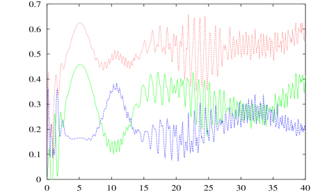
Figure 1: The total correlation for the system in excited state (a)$\frac{\Delta}{\lambda}=0.5$ (b) $\frac{\Delta}{\lambda}=1.0$ where $\bar{n}=10$.(C)$\frac{\Delta}{\lambda}=0.5$(d) $\frac{\Delta}{\lambda}=1$ where $\bar{n}=20$.

In Fig.(1), we assume that the qubits system is initially prepared in excited state i.e $\rho_{ab}(0)=|ee\rangle\langle ee|$. The effect of the detuning parameter $\Delta$ on the dynamics of correlation is shown in Figs.$(1a)$ and $(1b)$, where we plot the quantum, classical and the total correlations. It is clear that at $t=0$ the system is completely separable, so there is no any correlations between the two qubits. For a short period of time there is no quantum correlation but the classical and total correlations take place in a similar manner, $\mathcal{T}_{c}=\mathcal{C}_{c}$. As time evolves the quantum correlation appears and increases on the expanse of the classical correlation. At a certain range of time, the classical correlation exceeds the quantum correlation i. e $\mathcal{C}_{c}>\mathcal{Q}_{c}$, while for some other ranges $\mathcal{Q}_{c}>\mathcal{C}_{c}$. From theses figures we can see that for small values of the detuning parameter the quantum correlation tends to a minimum value while the classical correlation reaches to a maximum value at $\lambda t\simeq 10$ for Fig. $(1a)$.

The situation is changed considerably when the detuning is increased, where at the corresponding point which has been observed in Fig. $(1a)$, the minimum values of the quantum correlation increases on the expanse of the classical correlation. Also, the maximum values of $\mathcal{Q}_{c}$ as well as the intervals in which $\mathcal{C}_{c}>\mathcal{Q}_{c}$ decreases as the detuning parameter increases. These behaviors are seen by comparing Figs.($1a)$ and $(1b)$. The same remarks are seen in Figs.$(1c)$ and $(1d)$, where we consider $\bar{n}=20$. This means that as $\frac{\Delta}{\lambda}$ is increased a strong quantum correlation obtained, where the intervals of times in which $\mathcal{Q}_{c}>\mathcal{C}_{c}$ increase for large values of the detuning parameter So one can consider the detuning parameter as a control parameter to generate a long lived entanglement, where the two qubits entangled forever [15].

The effect of the mean photon number $\bar{n}$ is shown by comparing Figs. $(a,b)$ and Figs. $(c,d)$, where we assume that $\bar{n}=10,20$ respectively. From these figures the usual Rabi oscillation is seen, where the location of its oscillation is moved toward the positive direction as the time increases. Also, as the mean photon number increases the oscillations decreases and hence both classical and quantum correlations increase. This is clear by comparing Figs.$(1a)$ where we consider $\bar{n}=10$ and Fig.$(1c)$, where $\bar{n}=20$. We can see that although the maximum values of the $\mathcal{Q}_{c}$ decreases as $\bar{n}$ increases, the quantum correlations are more stable. This phenomena is seen clearly by comparing Figs.$(1b)$ and $(1d)$

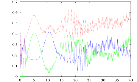
Figure 2: The total correlation for a system in ground state (a)$\frac{\Delta}{\lambda}=0.5$ and $\bar{n}=10$ (b) $\frac{\Delta}{\lambda}=1.0$ and $\bar{n}=20$

In Fig.$(2)$, we assume that the initial state of the atomic system is prepared in the ground state, $\psi_{AB}(0)=\bigl{|}gg\bigr{\rangle}$. By comparing the classical and quantum correlations in Fig. $(1a)$ and Fig. $(2a)$, one can see that the minimum value of the quantum correlation round $\lambda t=10$, in Fig.$(1a)$ is larger than that depicted on its corresponding at Fig.$(2a)$. Also, the intervals of times in which the quantum correlation is larger than the classical increases for the atomic system is prepared initially in the excited state Also, the same remark is seen in Fig. $(1d)$ and Fig. $(2b)$, where the minimum value of the quantum correlation in the later figure is smaller than that for Fig$.(1d)$.

From the preceding results, we can say that the quantum and classical correlations are sensitive for the detuning parameter, mean photon number and the initial state setting of the atomic system. One can recruitment these parameter to generate long-lived entangled state, where starting by atomic system in excited state, large detuning parameter and small mean photon number is one of the best choice to generate a useful entangled state for quantum information tasks.

Figure 3: The solid and dot curves represent the quantum and classical deficits for a system initially prepared in an excited state, where $\bar{n}=10$ and $\frac{\Delta}{\lambda}=0.5,1$ for Fig.(a) and Fig.(b) respectively.

4 Deficits

To measure how much of correlations that must be destroyed during the process of localizing information into a subsystem, we have to evaluate what is called quantum deficit. It is defined as the difference between the informational content in a state and information that can be localize to a subsystem by the use of local unitary operations and a dephasing channel [25]. The localizable information of a state $\varrho_{ab}$ is defined by the maximal amount of local information. In a mathematical form it is defined as,

$$\mathcal{I}_{loz}=Sup_{\Lambda\in LOCC}(\mathcal{I}(\varrho_{a})+\mathcal{I}(\varrho_{b})),$$ (9)

under the local operation and classical communication, LOCC. Then we can define the quantum deficit as

$$\mathcal{Q}_{def}=\mathcal{I}({\varrho_{AB}})-\mathcal{I}_{loz}.$$ (10)

Also in this context, it is important to evaluate the classical information deficit, $\mathcal{C}_{def}$. To achieve this aim we evaluate the local information, the total information which contained in the individual subsystems $\varrho_{a}$ and $\varrho_{b}$, $\mathcal{I}_{Lo}$. This quantity is defined by [25]-[27].

$$\mathcal{I}_{Lo}=\mathcal{I}(\varrho_{a})+\mathcal{I}(\varrho_{b})$$ (11)

Then the classical information deficit is,

$$\mathcal{C}_{def}=\mathcal{I}_{Loz}-\mathcal{I}_{Lo}.$$ (12)

This quantity quantify the amount of information that can be obtained from the state $\varrho_{ab}$ by exploiting additional correlations.

Given a specific initial state settings, it is known how to calculate the actual quantum and classical deficits in the interaction channel. Our investigation can be highlighted by a simple open question: what is the difference between highest quantum and classical deficits that will be obtained according different initial states? In Fig.$(3)$, we plot the quantum and classical deficits for the charged qubits system initially prepared in the excited state, $\bigl{|}\psi_{ab}(0)\bigr{\rangle}=\bigl{|}gg\bigr{\rangle}$ and the mean photon number $\bar{n}=10$, for different values of the detuning parameter. From this figure, it is clear that $\mathcal{Q}_{def}$ is zero for separable states at $\tau=0$. As the quantum correlation increase, the quantum deficit increases. This is because an entangled state is generated with high degree of entanglement. As an example at $\lambda t\simeq 5$, the generated entangled state has a high degree of entanglement and hence the $\mathcal{Q}_{def}$ increases. Also we can see that the quantum correlation is maximum round $\lambda t\simeq 20$ (see Fig. 1b). this means that an entangled state is generated with a high degree of entanglement. If we take a look at the same point in Fig.(3b), it is simply see that the quantum deficit is maximum, this is due to the weakness of the entanglement. So, one can say that for entangled states which have high degree of entanglement, the amount of information that destroyed in the process of localizing is much larger than for that observed in the less entangled states.

In Fig. $(4)$ we investigating a different setting of the charged qubit, where we consider the qubits are initially prepared in the ground state. The figure shows as one increases the detuning and the mean photon number the quantum deficit increases while the classical deficit decreases. This behavior due to the increasing of the degree of entanglement for these parameters.

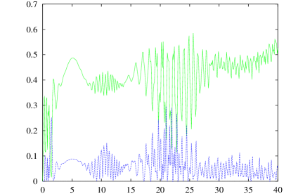
Figure 4: The same as Fig. (3), but for the charged qubits system is initially prepared in the ground state (a) For $\bar{n}=10$ and $\frac{\Delta}{\lambda}=0.5.$ (b) For $\bar{n}=20$ and $\frac{\Delta}{\lambda}=1.$

It would be interesting to study more deeply this phenomenon and understand better its connection to different kinds of entangled states. Hopefully, this will shed some light on the mysterious nature of multi-party correlations. Notice that there is a remarkable increases of the classical deficit $\mathcal{C}_{def}$ for less entangled states. This means that Alice and Bob can extract more information by means of the $CLOCC$ (classical communication and local operations). As an example around $\lambda t\simeq 5$, the classical correlation is minimum, so the amount of information that can be extracted in $CLOCC$ by Alice and Bob is minimum, while at $\lambda t\simeq 10$, where $\mathcal{C}_{c}$ is maximum, the classical deficit is maximum.

5 Conclusion

In conclusion, we have discussed quantum and classical information deficits of two superconducting charge qubits coupled with a common microwave resonator. It is shown that, under particular conditions, novel phenomena can be observed such as a strong quantum correlations, long-lived of entanglement and entangled states with high degree of entanglement generation. Moreover the enhancement of quantum correlation is much better than the classical correlations. Due to fragileness of the entanglement, the amount of information which has been destroyed in the process of localization increases for the generated entangled state has a high degree of entanglement. On the other hand, Alice and Bob can extract more information by using the local operation and classical communication for less entangled states. Also, theses results are very important in quantum cryptography, where if, we consider an eavesdropper(Eve) can make an additional measurement on the joint state between Alice and Bob, then the destroyed non-local information will increase for large detuning and small mean photon number.

References

- [1] C. J. Mewton and Z. Ficek, J. Phys. B 40, S181 (2007)
- [2] Y.A. Pashkin, T. Yamamoto, O. Astafiev, Y. Nakamura, D.V. Averin and J.S. Tsai, Nature, 421, 823, (2003).
- [3] M. Hentschel, D. C. B. Valente, E. R. Mucciolo, and H. U. Baranger, Phys. Rev. B 76, 235309 (2007)
- [4] D. D. Awschalom, D. Loss, and N. Samarth, (Springer, Berlin, 2002).
- [5] D. Loss and D. P. DiVincenzo, Phys. Rev. A 57, 120 (1998).
- [6] M. Riebe, M. Chwalla, J. Benhelm, H. Haeffner, W. Haensel, C. F. Roos, R. Blatt New J. Phys. 9, 211 (2007).
- [7] K. Hammerer, E.S. Polzik and J.I. Cirac Phys. Rev. A 74, 064301 (2007).
- [8] R. Perry, J. Opt. Soc. Am. B 22, 1561 (2005).
- [9] P. Garbaczewski, Appl. Math. Inf. Sci. 1, 1 (2007); N. Metwally, Int. J. Quant. Inf.,6 1, 187 - 200 (2008).
- [10] W. X.-Wen, L. Xiang and W. Yong, Phys. Lett. 24 11-14 (2007).
- [11] C. H. Bennett and G. Brassard, in Proceedings of IEEE International Conference on Computers, Systems, and Signal Processing (IEEE, 1984), pp. 175 – 179.
- [12] S.V. Prants, M.Yu. Uleysky and V.Yu. Argonov Phys. Rev. A.73 art. 023807 (2006).
- [13] X. Cui, S.-J. Gu, J. Cao, Y. Wang and H.-Q. Lin, J. Phys. A 40 13523 (2007).
- [14] L. Pankowski and B. Radtke, J. Phys. A, 41 075308 (2008).
- [15] M. Abdel-Aty, Phys. Lett. A , doi:10.1016/j.Physleta 200802017,(2008)
- [16] Y. Nakamura, Yu. A. Pashkin and J. S. Tsai, Nature, 398:786, (1999).
- [17] D. A. Rodrigues, C. E. A. Jarvis, B. L. Gyorffy, T. P. Spiller and J. F. Annett, J. Phys.: Cond. Matt. 20, 075211 (2008)
- [18] L. Henderson and V. Vedral, J. Phys. A 34, 6899 (2001); V. Vedral, Phys. Rev. Lett. 90, 050401 (2003); M. Abdel-Aty, Laser Physics Letters, 1, 104 (2004); F. N. M. Al-Showaikh, Appl. Math. Inf. Sci. 2, 21 (2008)
- [19] B. Groisman, S. Popescu and A. Winter Phys. Rev. A 72 032317 (2005).
- [20] W. L. Chan, J.-P. Cao, D. Yang and S.-J. Gu, J. Phys. A 4012143 (2007).
- [21] X. Cui, S-J. Gu, J. Cao, Y. Wang and H.-Q. Lin, J. Phys. A 40 13523 (2007).
- [22] S. Hill and W. K. Wootters phys. Rev. A 54 3624 (1996); W. K. Wootters, Phys. Rev. Lett. 80 2245, (1998).
- [23] K. Zyczkowski, P. Horodecki, A. Sanpera and M. Lewenstein, Phys. Rev. A 58, 883 (1998).
- [24] A. Gogo, W. D. Snyder, and M. Beck, Phys. Rev. A 71, 052103 (2005).
- [25] J. Oppenheim, M. Horodecki, P. Horodecki and R. Horodecki, Phys. Rev. Lett. 89 180402 (2002).
- [26] B. Synak and M. Horodecki, J. Phys. A: Math. Gen. 37 11465-11474 (2004).
- [27] M. Horodecki, P. Horodecki, R. Horodecki, J. Oppenheim, A. Sen De, U. Sen, and B. Synak, Phys. Rev. A 71, 062307 (2005).