Pre-equilibrium dilepton production from an anisotropic quark-gluon plasma
Abstract
We calculate leading-order dilepton yields from a quark-gluon plasma which has a time-dependent anisotropy in momentum space. Such anisotropies can arise during the earliest stages of quark-gluon plasma evolution due to the rapid longitudinal expansion of the created matter. Two phenomenological models for the proper time dependence of the parton hard momentum scale, , and the plasma anisotropy parameter, , are constructed which describe the transition of the plasma from its initial non-equilibrium state to an isotropic thermalized state. The first model constructed interpolates between 1+1 dimensional free streaming at early times and 1+1 dimensional ideal hydrodynamical expansion at late times. In the second model we include the effect of collisional broadening of the parton distribution functions in the early-time pre-equilibrium stage of plasma evolution. We find for both cases that for fixed initial conditions high-energy dilepton production is enhanced by pre-equilibrium emission. When the models are constrained to fixed final pion multiplicity the dependence of the resulting spectra on the assumed plasma isotropization time is reduced. Using our most realistic collisionally-broadened model we find that high-transverse momentum dilepton production would be enhanced by at most 40% at the Relativistic Heavy Ion Collider and 50% at CERN Large Hadron Collider if one assumes an isotropization/thermalization time of 2 fm/c. Given sufficiently precise experimental data this enhancement could be used to determine the plasma isotropization time experimentally.
pacs:
11.15Bt, 04.25.Nx, 11.10Wx, 12.38MhI Introduction
With the ongoing ultrarelativistic heavy ion collision experiments at RHIC and future experiments planned at LHC the goal is to produce a deconfined plasma of quarks and gluons (QGP). This new state of matter is expected to be formed once the temperature of nuclear matter exceeds the critical temperature, 200 MeV. However, many properties of the expected QGP are still poorly understood. One of the most difficult problems is the determination of the isotropization and thermalization time of the QGP, and , respectively.111For simplicity from here forward we will assume that these two time scales are the same, , so that the system achieves isotropization and thermalization at the same proper time given by . At RHIC energies it was found that, for 2 GeV, the plasma elliptic flow, , was well described by ideal hydrodynamical models. Based on early studies Huovinen:2001cy ; Hirano:2002ds ; Tannenbaum:2006ch ideal hydrodynamical fits to elliptic flow data indicated that the matter can be modeled as a nearly-perfect fluid starting at extremely early times after the collision, 0.6 fm/c Huovinen:2001cy . However, recent hydrodynamical studies Luzum:2008cw which include the effect of all 2nd-order transport coefficients consistent with conformal symmetry have shown that these initial estimates for the isotropization/thermalization time of the plasma have a sizable uncertainty due to poor knowledge of the proper initial conditions (CGC versus Glauber), details of plasma hadronization and subsequent hadronic cascade, etc. As a result, it now seems that isotropization times up to 2 fm/c are not ruled out by RHIC data and in order to further constrain this time additional theoretical and experimental input will be required.
As mentioned above there are uncertainties introduced in hydrodynamic modeling of the quark-gluon plasma (QGP) due primarily to the dependence of the results on the assumed initial conditions: initial energy density, spatial profile, flow velocity, etc. In order to remove this uncertainty one would like to find observables which are sensitive to the earliest times after the collision and are relatively unaffected by the later stages of plasma evolution. One obvious candidate to consider is high-energy dilepton production since dileptons couple only electromagnetically to the plasma and therefore, in their high-energy spectra, carry information about plasma initial conditions. To this end here we calculate the dependence of leading-order high-energy dilepton production on the assumed isotropization and thermalization time of the QGP using two simple models for early-time QGP evolution.
To begin the discussion we introduce two proper time scales: (1) the parton formation time, , which is the time after which one can treat the partons generated from the nuclear collision by a distribution of on-shell partons; and (2) the isotropization time, , which is the time when the system becomes isotropic in momentum-space. At RHIC energies fm/c and at LHC energies fm/c. Immediately after the collision, the partons are produced from the incoming colliding nuclei at , at which time the partonic momentum distributions can be assumed to be isotropic.222See Ref. Jas:2007rw for an alternative view of the early times after the initial collision wherein the authors find that the distribution may be prolate for longer than assumed here. We postpone the study of the possibility of early-time prolate distributions to future work. The subsequent rapid longitudinal expansion of the matter (along the beam line) causes it to become much colder in the longitudinal direction than in the transverse direction Baier:2000sb . Longitudinal cooling occurs because initially the longitudinal expansion rate is larger than the parton interaction rate and, as a result, a local momentum-space anisotropy is induced with in the local rest frame. If the system is to return to an isotropic state it is necessary that at some later time the interaction rate overcomes the expansion rate with the system finally isotropizing and remaining isotropic for . Once isotropy is achieved (and maintained by parton interactions) the use of hydrodynamic simulations can be justified. We are therefore critically interested in the properties of the plasma around the isotropization time as these provide the relevant initial conditions for subsequent hydrodynamic evolution.
The study of anisotropic plasmas has received much interest recently due to the fact that a quark-gluon plasma which has a local momentum-space anisotropy, , is subject to the chromo-Weibel instability Strickland:2007fm ; Mrowczynski:2000ed ; Randrup:2003cw ; Romatschke:2003ms ; Arnold:2003rq ; Romatschke:2004jh ; Mrowczynski:2004kv ; Rebhan:2004ur ; Arnold:2005vb ; Arnold:2004ti ; Rebhan:2005re ; Romatschke:2005pm ; Schenke:2006xu ; Schenke:2006fz ; Manuel:2006hg ; Bodeker:2007fw ; Romatschke:2006nk ; Romatschke:2006wg ; Dumitru:2005gp ; Dumitru:2006pz ; Rebhan:2008uj . The chromo-Weibel instability causes rapid growth of soft gauge fields which preferentially work to restore the isotropy of the quark-gluon plasma on time scales much shorter than the collisional time scale. However, most of the theoretical and numerical developments in describing the time-evolution of a QGP subject to the chromo-Weibel instability have been restricted to asymptotic energies at which perturbative resummations can be applied and hence the presence of the instability-driven isotropization at RHIC and LHC energies is not yet proven. In addition, numerical studies of the chromo-Weibel instability in an 1-dimensionally expanding system show that there is a time delay before the effects of plasma instabilities become important to the system’s dynamics Romatschke:2006wg ; Rebhan:2008uj . Future work will address these issues but until they become available there is a substantial amount of theoretical uncertainty in the QGP isotropization time, 3 fm/c.
In the absence of a precise physical framework for describing the thermalization of the quark-gluon plasma and the associated time scales, one possible way to proceed is by studying the dependence of observables sensitive to the earliest times after the collision on the assumed plasma isotropization time by constructing simple space-time models. As mentioned above, one candidate observable is electromagnetic radiation such as high-energy photon and dilepton production333Hereafter, high-energy dileptons will refer to lepton pairs with pair transverse momentum () or invariant mass () greater than 1 GeV. since these particles interact only electromagnetically and can escape from the strongly interacting medium created after the collision unhindered. Hence, they are perfect probes for studying the early-time dynamics of the system. In the case of high-energy medium photon production it is difficult for experimentalists to subtract the large backgrounds coming from decays from other sources of photons, making it hard to measure a clean high-energy medium photon production signal.444For a discussion of the effect of possible momentum-anisotropies on high-energy photon production see Ref. Schenke:2006yp . In the case of high-energy dileptons, the experimental situation is dramatically improved and it then becomes a question of making the necessary theoretical predictions to see how large the effect of a possible anisotropic pre-equilibrium phase would be on dilepton production.
Phenomenological studies of the production of high-energy dileptons have shown that there are several important dilepton sources and it’s necessary to include each of these depending on the kinematic region. For dilepton pair transverse momentum or invariant mass greater than 1 GeV the most important sources of dilepton pairs are: charm quark decays, initial state Drell-Yan scatterings, jet-conversion, jet-fragmentation, and medium (thermal) production. For an extensive discussion of the various sources of the dilepton production in a heavy-ion collision, we refer the reader to Gale:2003iz ; Turbide:2006zz and references therein. Note that in most previous phenomenological studies of photon and dilepton production it has been assumed that the system “instantaneously” thermalizes with and hence is locally isotropic throughout its evolution.
In this paper, we extend our previous work Mauricio:2007vz and concentrate on the impact of momentum-space anisotropies on the leading order medium dilepton production at large invariant mass and transverse momentum. We propose two simple phenomenological models for the time dependence of the plasma momentum-space anisotropy, , and hard momentum scale, . In the first model we interpolate between 1+1 dimensional longitudinal free-streaming and 1+1 dimensional ideal hydrodynamic expansion. In the second model we incorporate the effect of momentum-space broadening due to hard-hard elastic scatterings in the pre-equilibrium dynamics.555We will assume that this elastic scattering rate is regulated in the infrared by an isotropic screening mass for simplicity. In both models we introduce two parameters, and , with setting the width of the transition from early-time pre-equilibrium dynamics to late-time equilibrated dynamics. In the limit our models reduce to ideal 1+1 dimensional hydrodynamical expansion and in the opposite limit correspond to two different types of non-equilibrium plasma evolution: free streaming expansion or collisionally-broadened expansion.
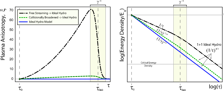
In Fig. 1 we sketch the proper time dependence of the plasma anisotropy parameter, , and energy density in the three cases considered below: free-streaming followed by ideal hydrodynamic expansion, collisionally broadened expansion followed by ideal hydrodynamic expansion, and “instantaneous” thermalization (ideal hydro throughout evolution). As can be seen from this figure for both the free streaming and collisionally-broadened cases with fixed initial conditions the energy density is always greater than that obtained by a system undergoing ideal hydrodynamic evolution and therefore one expects that, for fixed initial conditions, non-equilibrium effects can significantly enhance dilepton production. In order to calculate just how much the signal is enhanced requires detailed calculations which we present below. As our first result we will show that for fixed initial conditions the addition of a pre-equilibrium phase at times enhances high-energy dilepton production by up to an order of magnitude.
We then study the effect of constraining our space-time models so that the initial conditions vary in order to guarantee that the final pion multiplicity is independent of the assumed isotropization/thermalization time. We show that allowing the initial conditions to vary in this way reduces the final effect of the possible anisotropic pre-equilibrium phase. In order to quantify the effect we introduce a ratio called the “dilepton enhancement”, , which is the ratio of the dilepton yield obtained when one assumes a finite isotropization/thermalization time to that obtained when one assumes that the plasma “instantaneously” thermalizes at the formation time, . We show that, in our most realistic collisionally-broadened model, the dilepton enhancement can be up to 40% at RHIC energies and 50% at LHC energies if one assumes a isotropization/thermalization time of 2 fm/c. We also show that as one varies the assumed isotropization/thermalization time that the dilepton enhancement, , has a non-trivial dependence on pair transverse momentum which could allow experimental determination of if the experimental medium dilepton yields are obtained with high enough precision.
The work is organized as follows: In Sec. II we calculate the dilepton production rate at leading order using an anisotropic phase space distribution. In Sec. III we construct models which interpolate between anisotropic and isotropic plasmas. In Sec. IV we present our final results on the dependence of dilepton production on the assumed plasma isotropization time and compare with other relevant sources of high-energy dileptons. Finally, we present our conclusions and give an outlook in the Sec. V.
II Dilepton Rate from Kinetic Theory
From relativistic kinetic theory, the dilepton production rate (i.e. the number of dileptons produced per space-time volume and four dimensional momentum-space volume) at leading order in the electromagnetic coupling, , is given by Kapusta:1992uy ; Dumitru:1993vz ; Strickland:1994rf :
| (1) |
where is the phase space distribution function of the medium quarks (anti-quarks), is the relative velocity between quark and anti-quark and is the total cross section
| (2) |
where is the lepton mass and is the center-of-mass energy. Since we will be considering high-energy dilepton pairs with center-of-mass energies much greater than the dilepton mass we can safely ignore the finite dilepton mass corrections and use simply . In addition, to very good approximation we can assume that the distribution function of quarks and anti-quarks is the same, .
In this work we will assume azimuthal symmetry of the matter in momentum-space so that the anisotropic quark/anti-quark phase distributions can be obtained from an arbitrary isotropic phase space distribution by squeezing () or stretching () along one direction in the momentum space, i.e.
| (3) |
where is the hard momentum scale, is the direction of the anisotropy and is a parameter that reflects the strength and type of anisotropy. In general, is related to the average momentum in the partonic distribution function. In isotropic equilibrium, where =0, can be identified with the plasma temperature . To give another specific example, in the case of 1+1 dimensional free-streaming discussed in Sec. III.1.2 is given by the initial “temperature” .
For general we split the delta function in Eq. (1) such that we can perform the integration:
| (4) | |||||
Choosing spherical coordinates with the anisotropy vector defining the axis, we can write:
| (5) |
It is then possible to reexpress the remaining delta function as:
| (6) |
with . The angles are defined as the solutions to the following transcendental equation:
| (7) |
We point out that there are two solutions to Eq. (7) when . After these substitutions and expanding out the phase space integrals, we obtain:
| (8) | |||||
with
| (9) |
Note that when , the limit of isotropic dilepton production is recovered trivially. Also note that as increases we expect the differential dilepton rate to decrease since for fixed the increasing oblateness of the parton distribution functions causes the effective parton density to decrease:
| (10) | |||||
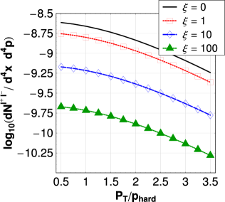
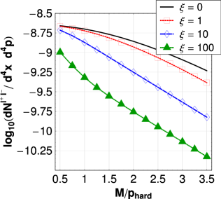
In order to evaluate the anisotropic dilepton rate it is necessary to perform the remaining two integrations in Eq. (8) numerically. In Fig. 2 we plot the resulting differential dilepton rate as a function of transverse momentum and invariant mass for . One can see the effect of increasing for fixed , namely that the dilepton production rate decreases due, primarily, to the density effect mentioned above.
Knowing the rate, however, is not enough to make a phenomenological prediction for the expected dilepton yields. For this one must include the space-time dependence of and and then integrate over the space-time volume
| (11a) | ||||
| (11b) | ||||
where fm is the radius of the nucleus in the transverse plane. These expressions are evaluated in the center-of-mass (CM) frame while the differential dilepton rate is calculated for the local rest frame (LR) of the emitting region. Then, the dilepton pair energy has to be understood as in the differential dilepton rate . Additionally, in Eqs. (11) we have assumed that there is only longitudinal expansion of the system. Since at early times the transverse expansion is small compared to the longitudinal expansion, one can ignore it. Some studies have suggested that the influence of the transverse expansion on the space-time evolution becomes phenomenologically important around 2.7 fm/c Ollitrault:2007du , therefore, our approximation is valid for describing the early-time behaviour we are interested in. Substituting Eq. (8) into Eqs. (11) we obtain the dilepton spectrum including the effect of a time-dependent momentum anisotropy.
Note that we have not included the next-to-leading order (NLO) corrections to the dilepton rate due to the complexity of these contributions for finite . These affect dilepton production for isotropic systems for 1 Thoma:1997dk ; Arnold:2002ja ; Arleo:2004gn ; Turbide:2006mc . In the regions of phase space where there are large NLO corrections, we will apply -factors to our results as indicated. These -factors are determined by taking the ratio between NLO and LO calculation for an isotropic plasma, therefore, in this work we are implicitly assuming that the -factor will be the same for an anisotropic plasma.
III Space-Time Models
In this section we present two new models for 1+1 dimensional non-equilibrium time-evolution of the QGP and review the cases of 1+1 dimensional free-streaming and 1+1 dimensional hydrodynamic expansion. In all cases considered below the number density will obey in its asymptotic regions.666The interpolating models will only obey this relation outside of a region of order around where the transition between different types of expansion takes place. In the transition region will increase due to non-equilibrium effects as we discuss later in the text. This results in all cases from the assumption that the total particle number is fixed while the size of the box containing the plasma is expanding at the speed of light in the longitudinal direction (1d expansion).
In each case below we will be required to specify a proper time dependence of the hard-momentum scale, , and anisotropy parameter, , which is consistent with this scaling for and . Before proceeding, however, it is useful to note some general relations. Firstly we remind the reader that the plasma anisotropy parameter is related to the average longitudinal and transverse momentum of the plasma partons via the relation
| (12) |
Therefore, we can immediately see that for an isotropic plasma that , and for an oblate plasma which has that .
Secondly we note that given any anisotropic phase space distribution of the form specified in Eq. (3) the local energy density can be factorized via a change of variables to give
| (13) | ||||
where is the initial local energy density deposited in the medium at and
| (14) |
We note that and .
III.1 Asymptotic Limits of the Anisotropic Phase Space Distribution
Before presenting our proposed interpolating models we review previous calculations for the free streaming and hydrodynamic expansion cases Kapusta:1992uy ; Kampfer:1992bb ; Kajantie:1986dh and show how to determine our anisotropic phase space distribution function parameters, and , in these two cases.
III.1.1 1+1 Dimensional Ideal Hydrodynamical Expansion Limit
We first consider the limiting case that so that the plasma is assumed to be “instantaneously” thermal and isotropic and undergoes ideal 1+1 dimensional hydrodynamical expansion throughout its evolution. In ideal hydrodynamical evolution using the boost-invariant 1+1 Bjorken model Bjorken:1982qr we can identify with the temperature and the anisotropy parameter vanishes by assumption, . Due to the fact that the distribution function for highly relativistic particles will depend only on the ratio between the energy and temperature, with . In this case the number density, hard scale (temperature), energy density, and anisotropy parameter obey the following
| (15a) | |||||
| (15b) | |||||
| (15c) | |||||
| (15d) | |||||
In order to obtain an analytic result for the differential dilepton rate which is applicable at high energies one can approximate the quark and anti-quark Fermi-Dirac distributions by Boltzmann distributions and integrate Eq. (8) analytically. In this case it is also possible to perform the necessary integration of the rate over the plasma space-time evolution analytically Kapusta:1992uy ; Kajantie:1986dh to obtain:
| (16a) | ||||
| (16b) | ||||
where , and . As a check of our numerics we have verified that numerical integration of our dilepton rate given in Eq. (8) over space-time via Eqs. (11) reproduces this analytic result in the limit and .
III.1.2 1+1 Dimensional Free Streaming Limit
As another limiting case we can assume instead that our 1+1 dimensional expanding plasma is non-interacting. If this were true then the system would simply undergo 1+1 dimensional free-streaming expansion Kapusta:1992uy ; Kampfer:1992bb . Since, in this case, the system would never become truly thermal or isotropic this corresponds to taking the opposite limit from the one we took in the previous subsection, namely we will now take the limit .
In the free streaming case, the distribution function is a solution of the collisionless Boltzmann equation
| (17) |
where the subscript indicates that this is the free-steaming solution. In this work we will also assume that the distribution function is isotropic at the formation time, .
| (18) |
where is the transverse momentum, is the longitudinal momentum and is the hard momentum scale at . The typical hard momentum scale of particles undergoing 1+1 dimensional free streaming expansion is constant in time. In the case of indefinite free-streaming expansion the system never reaches thermal equilibrium and so the system strictly cannot have a temperature associated with it; however, since our assumed distribution function is isotropic at , we can identify the initial “temperature” of the system, , with the hard momentum scale when comparing hydrodynamic and free streaming expansion.
Eq. (17) has a family of solutions which are boost invariant along the (beam) axis
| (19) |
Therefore, the functional dependence of the distribution function for the free streaming case is of the form
| (20) |
This distribution function can be simplified if we change to co-moving coordinates:
| (21a) | ||||
| (21b) | ||||
where, as usual, is the momentum-space rapidity, is the proper time, and is the space-time rapidity. In terms of these variables one obtains
| (22) |
Note that in the case of indefinite free-streaming at late times the quark and anti-quark longitudinal momentum are highly red-shifted reducing late time emission of high-energy dilepton pairs.
As written in Eq. (12) the anisotropy parameter is related with the average transverse and longitudinal momenta of the partons. The average momentum-squared values appearing there are defined in the standard way:
| (23) |
Using the 1+1 dimensional free streaming distribution given in Eq. (22) and transforming to co-moving coordinates defined in (21) so that we obtain
| (24a) | ||||
| (24b) | ||||
Inserting these expressions into the general expression for given in Eq. (12) one obtains . With this in hand we can also determine proper time dependence of the energy density in the free-streaming case by substituting this expression for into Eq. (13), . At early times one must use the full expression given by Eq. (13); however, at late times one can expand this result to obtain as expected for a 1+1 free streaming plasma Baym:1984np .
Summarizing, one finds in the 1+1 free streaming case that in the limit :
| (25a) | |||||
| (25b) | |||||
| (25c) | |||||
| (25d) | |||||
With the distribution function given by Eq. (22), the dilepton spectrum can be calculated. As a function of the invariant mass , one obtains
| (26) |
In the last expression, the integration is over all from 0 to and over all from to subject to the constraint
As a function of the transverse momentum, , the dilepton production using free streaming case we obtain777In the original article by Kapusta et. al Kapusta:1992uy , the calculation of was not presented.
| (27) |
with
| (28) |
We have verified that using the expressions listed in Eq. (25) our direct numerical integration of the rate given in Eq. (8) over space-time via Eqs. (11) reproduces this analytic result in the free-streaming limit.
We note in closing that as a solution of the collisionless (non-interacting) Boltzmann equation, the free-streaming case can be taken as an upper bound on the magnitude of the plasma anisotropy parameter since for fixed (no transverse expansion/contraction) cannot be larger than the free-streaming value by causality.
III.2 Momentum-space Broadening in a 1+1 Dimensionally Expanding Plasma
In the previous two subsections we presented details of the limiting cases for 1+1 dimensional plasma evolution: 1+1 ideal hydrodynamic expansion and 1+1 dimensional free streaming, with the former arising if there is rapid thermalization of the plasma and the latter arising if the plasma has no interactions. We would now like to extend these models to include the possibility of momentum-space broadening of the plasma partons due to interactions (hard and soft). This can be accomplished mathematically by generalizing our expression for to
| (29) |
In the limit , and one recovers the 1+1 hydrodynamical expansion limit and in the limit one recovers the 1+1 dimensional free streaming limit, For general between these limits one obtains the proper time dependence of the energy density and temperature by substituting (29) into the general expression for the factorized energy density (13) to obtain . In the limit this gives the following scaling relations for the number density, energy density, and hard momentum scale
| (30a) | |||||
| (30b) | |||||
| (30c) | |||||
Different values of arise dynamically from the different processes contributing to parton isotropization. Below we list the values of resulting from processes which are relevant during the earliest times after the initial nuclear impact.
III.2.1 Collisional Broadening via Elastic 22 collisions
In the original version of the bottom up scenario Baier:2000sb , it was shown that, even at early times after the nuclear impact, elastic collisions between the liberated partons will cause a broadening of the longitudinal momentum of the particles compared to the non-interacting, free-streaming case. During the first stage of the bottom-up scenario, when , the initial hard gluons have typical momentum of order and occupation number of order . Due to the fact that the system is expanding at the speed of light in the longitudinal direction . If there were no interactions this expansion would be equivalent to 1+1 free streaming and the longitudinal momentum would scale like . However, when elastic collisions of hard gluons are taken into account Baier:2000sb , the ratio between the longitudinal momentum and the typical transverse momentum of a hard particle decreases as:
| (31) |
Assuming, as before, isotropy at the formation time, , this implies that for a collisionally-broadened plasma . Note that, as obtained in Ref Baier:2000sb , the derivation of this result makes an implicit assumption that the elastic cross-section is screened at long distances by an isotropic real-valued Debye mass. This is not guaranteed in an anisotropic plasma as the Debye mass can be become complex due to the chromo-Weibel instability Romatschke:2003ms . However, at times short compared to the time scale where plasma instabilities become important we expect the isotropic result to hold to good approximation.
III.2.2 Effect of Plasma Instabilities
Plasma instabilities affect the first stage of bottom-up scenario Arnold:2003rq . These instabilities are characterized by the growing of chromo-electric and -magnetic fields and . These fields bend the particles and how much bending occurs will depend on the amplitude and domain size of the induced chromofields. Currently, the precise parametric relations between the amount of plasma anisotropy and amplitude and domain size of the chromofields are not known from first principles. There are three possibilities for how the chromo-Weibel instability will affect isotropization of a QGP proposed in the literature Bodeker:2005nv ; Arnold:2005qs ; Arnold:2007cg :
| (32) |
where
| (33) |
These results correspond to , , and , respectively.
III.2.3 Summary and Discussion
Summarizing, the coefficient takes on the following values
| (34) |
The exponents in Eq. (34) are direct consequence of the relation between the anisotropy parameter and the longitudinal and transverse momentum given in Eq. (12). The exponent indicates which kind of broadening we are considering. Notice that =2 (0) reproduces the behaviour of free streaming (hydrodynamic) expansion.
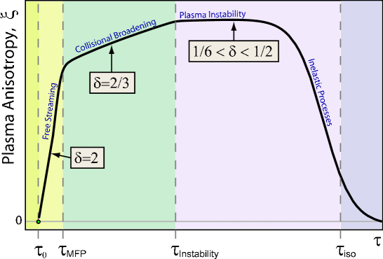
In Fig. 3 we sketch the time-dependence of the plasma anisotropy parameter indicating the time scales at which the various processes become important. At times shorter than the mean time between successive elastic scatterings, , the system will undergo 1+1 dimensional free streaming with . For times long compared to but short compared to the plasma anisotropy will grow with the collisionally-broadened exponent of . Here is the time at which instability-induced soft gauge fields begin to influence the hard-particles’ motion. When the plasma anisotropy grows with the slower exponent of due to the bending of particle trajectories in the induced soft-field background. At times large compared to inelastic processes are expected to drive the system back to isotropy Baier:2000sb . We note here that for small and realistic couplings it has been shown Schenke:2006xu that one cannot ignore the effect of collisional-broadening of the distribution functions and that this may completely eliminate unstable modes from the spectrum.
Based on such a sketch one could try to construct a detailed model which includes all of the various time scales and study the dependence of the process under consideration on each. However, due to the current theoretical uncertainties in each of these time scales and their dependences on experimental conditions we choose to use a simpler approach in which we will construct two phenomenological models which smoothly interpolate the coefficient :
| Free streaming interpolating model : | |||
| Collisionally-broadened interpolating model : |
In both models we introduce a transition width, , which governs the smoothness of the transition from the initial value of to at . The free streaming interpolating model will serve as an upper-bound on the possible effect of early time momentum-space anisotropies while the collisionally-broadened interpolating model should provide a more realistic estimate of the effect due to the lower anisotropies generated. This will help us gauge our theoretical uncertainties. Note that by using such a smooth interpolation one can achieve a reasonable phenomenological description of the transition from non-equilibrium to equilibrium dynamics which should hopefully capture the essence of the physics. In the next section we will give mathematical definitions for these two models.
III.3 Space-Time Interpolating Models with Fixed Initial Conditions
In order to construct our interpolating models, the parameter should be a function of proper time. To accomplish this, we introduce a smeared step function
| (35) |
where sets the width of the transition between non-equilibrium and hydrodynamical evolution in units of .888Note that compared to Ref. Mauricio:2007vz we have modified our definition of so that it now measures the width in units of instead of . This results in time-dependence of modeled quantities not experiencing unphysical “dips” which can occur for large values of in our previous interpolating model AndiPersonal . In the limit when , we have and when we have .
Physically, the energy density should be continuous as we change from the initial non-equilibrium value of to the final isotropic value appropriate for ideal hydrodynamic expansion. Once the energy density is specified this immediately gives us the time dependence of the hard momentum scale. We find that for general this can be accomplished with the following model
| (36a) | ||||
| (36b) | ||||
| (36c) | ||||
with defined in Eq. (14) and for fixed initial conditions
| (37a) | |||||
| (37b) | |||||
The power of in keeps the energy density continuous at for all . In the following subsections we will briefly discuss the two interpolating models we consider in this work.
III.3.1 Free streaming interpolating model
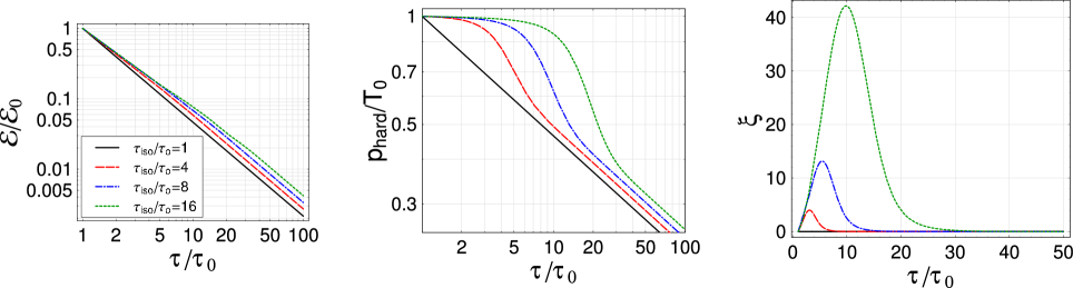
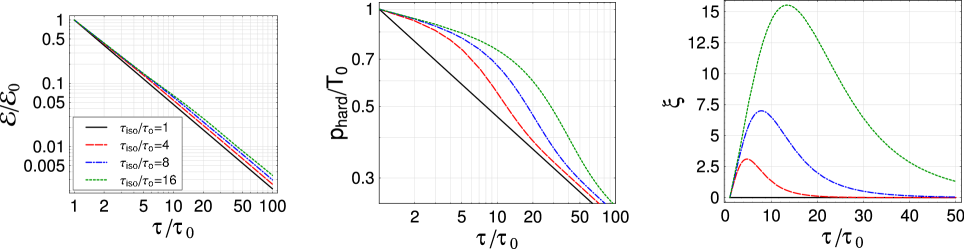
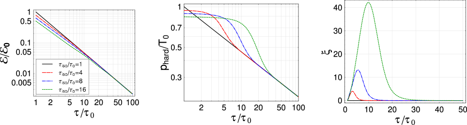
Using Eq. (36) we can obtain a model which interpolates between early-time 1+1 dimensional longitudinal free streaming and late-time 1+1 dimensional ideal hydrodynamic expansion by choosing . With this choice and in the limit , we have and the system undergoes 1+1 dimensional free streaming. When then and the system is expanding hydrodynamically. In the limit , , the system makes a theta function transition from free streaming to hydrodynamical evolution with the energy density being continuous during this transition by construction. In Fig. 4 we plot the time-dependence of , , and assuming (top) and (bottom) for different values of . As can be seen from this figure for fixed initial conditions during the period of free-streaming evolution the system always has a higher effective temperature () than would be obtained by a system which undergoes only hydrodynamic expansion from the formation time. As we will show in the results section, for fixed initial conditions, this results in a sizable enhancement in high-energy dilepton production.
III.3.2 Collisionally-broadened interpolating model
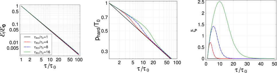
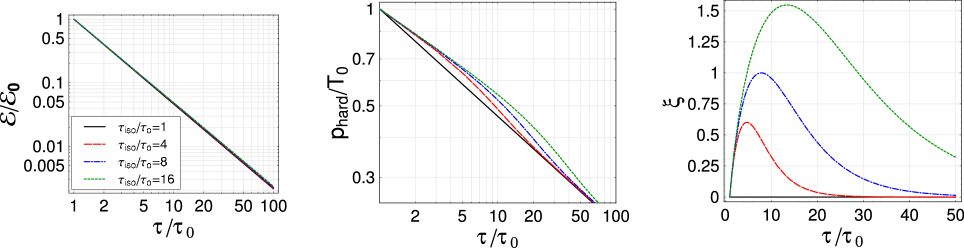
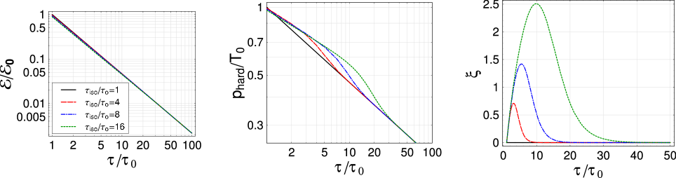
Similarly using Eq. (36) we can obtain a model which interpolates between early-time 1+1 dimensional collisionally-broadened expansion and late-time 1+1 dimensional ideal hydrodynamic expansion by choosing . In Fig. 5 we plot the time-dependence of , , and assuming (top) and (bottom) for different values of . As in the free-streaming interpolating model for fixed initial conditions at early times a collisionally-broadened system always has a higher effective temperature () than would be obtained by a system which undergoes only hydrodynamic expansion from the formation time. As we will show in the results section, for fixed initial conditions, this results in an enhancement in high-energy dilepton production; however, compared to the free-streaming case the effect is reduced due to the lower effective temperatures obtained by the collisionally-broadened plasma. We also note that in the case of collisionally-broadened expansion the magnitude of is significantly reduced as compared to the free-streaming case. As can be seen from the rightmost panel of Fig. 5 even if one assumes a large isotropization time, , the amount of momentum space anisotropy generated is small with for and for .
| Interpolating Model | RHIC – 10% | RHIC – 20% | LHC – 10% | LHC – 20% |
|---|---|---|---|---|
| Free-Streaming () | 0.8 fm/c | 1.2 fm/c | 0.26 fm/c | 0.4 fm/c |
| Collisionally-Broadened () | 5 fm/c | 18 fm/c | 1.6 fm/c | 6.2 fm/c |
III.4 Space-Time Interpolating Models with Fixed Final Multiplicity
In the previous subsection we constructed models which allow one to interpolate between an initially non-equilibrium plasma to an isotropic equilibrium one assuming that the initial conditions are held fixed. One problem with this procedure is that given fixed initial conditions these interpolating models will result in generation of particle number during the transition from to zero.
One can derive an expression for the amount by which the number density is increased by starting from the general expression for the particle number density and using the expression for derived in the previous section (36c) to obtain
| (38) |
Taking the limit we obtain
| (39) |
Translating this into a statement about the entropy generation using gives
| (40) |
When either or , goes to zero and there is no entropy generation; however, entropy generation increases monotonically with . In the limit of large we find
| (41) |
Again we see that in the limit that either or then there is no entropy generation.
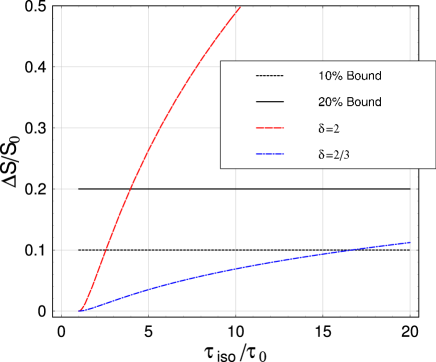
The requirement of bounded entropy generation can be used to constrain non-equilibrium models of the QGP Dumitru:2007qr . In Fig. 6 we plot the entropy generation (particle number generation) resulting from our models using Eq. (40) for along with bounds at 10% and 20%. In the free-streaming interpolating model () with fixed initial conditions requiring that the percentage entropy generation be less than each of these bounds requires for the 10% bound and for the 20% bound. In the collisionally-broadened interpolating model () with fixed initial conditions we obtain similarly for the 10% bound and for the 20% bound. We summarize our results in Table 1. As can be seen from Table 1 requiring the listed bounds on entropy generation the values of allowed in our free-streaming interpolating model become highly constrained. However, in the case of the collisionally-broadened interpolating model the upper-bounds imposed on are much larger due to the much lower entropy generation required to transition from collisionally-broadened evolution to hydrodynamic evolution.
One problem with our fixed initial condition family of models is that due to the fact that they generate additional particles the multiplicity of final particles is not independent of the assumed value of . Because most of the experimental results for dilepton spectra are binned with respect to a fixed final multiplicity this means that we should also construct models which always result in a fixed final number density. In the following subsection we will show how this can be accomplished.
III.4.1 Enforcing Fixed Final Multiplicity
We will now construct interpolating models which have a fixed final entropy (multiplicity). In order to accomplish this the initial conditions will have to vary as a function of the assumed isotropization time. We will show that, as a result, for finite one must lower the initial “temperature” in both the free-streaming and collisionally-broadened interpolating models. To accomplish this requires only a small modification to the definition of in Eq. (37):
| (42a) | |||||
| (42b) | |||||
As a consequence of this modification, the initial energy density and hence initial “temperature” will depend on the assumed value for . There is no modification required for . We demonstrate this in Fig. 7 where we plot the time-dependence of , , and for and (top) and (bottom) .
In the remainder of this work we present our final results for dilepton yields using both approaches, i.e., fixed initial conditions using Eqs. (36) with (37) or fixed final multiplicity through Eq. (36) with (42). We mention that in both cases, dilepton production is affected in the presence of anisotropies in momentum-space, however, one anticipates that the effect will be larger when the initial conditions are held fixed due to the larger particle number generation. We will come back to this issue in the conclusions and discussion.
IV Results
In this section we will present expected yields resulting from a central Au-Au collision at RHIC full beam energy, =200 GeV and from a Pb-Pb collision at LHC full beam energy, =5.5 TeV. In all figures in this section we will present the prediction for RHIC energies in the left panel and LHC energies in the right panel.
Before presenting our results we first explain the setup, numerical techniques used, and parameters chosen for our calculations. Because the differential dilepton rate given in Eq. (8) is independent of the assumed space-time model. We first evaluate it numerically using double-exponential integration with a target precision of . The result for the rate was then tabulated on a uniformly-spaced 4-dimensional grid in , , , and : , , . This table was then used to build a four-dimensional interpolating function which was valid at continuous values of these four variables. We then boost this rate from the local reference frame to center-of-mass frame and evaluate the remaining integrations over space-time ( and ) and transverse momentum or invariant mass appearing in Eqs. (11) using quasi-Monte Carlo integration with , and, depending on the case, restrict the integration to any cuts specified in or . Our final integration time, , is set by solving numerically for the point in time at which the temperature in our interpolating model is equal to the critical temperature, i.e. . We will assume that when the system reaches , all medium emission stops. We are not taking into account the emission from the mixed/hadronic phase at late times since the kinematic regime we study (high and ) is dominated by early-time high-energy dilepton emission Strickland:1994rf ; Mauricio:2007vz .
For RHIC energies we take an initial temperature = 370 MeV, at a formation time of = 0.26 fm/c, and use = 6.98 fm. For LHC energies, we use = 0.088 fm/c, = 845 MeV and = 7.1 fm. In both cases, the critical temperature is taken as 160 MeV and the spectra are calculated at midrapidity region . Any cuts in transverse momentum or invariant mass will be indicated along with results. Note that the precise numerical value of the parameters above were chosen solely in order to facilitate straightforward comparisons with previous works Turbide:2006mc from which we have obtained predictions for Drell Yan, heavy quark, jet-fragmentation, and jet-thermal dilepton yields.
Finally we note that below we will use -factors to adjust for next-to-leading order corrections to the dilepton rate. These -factors are determined by computing the ratio of the next-to-leading order prediction of Arnold:2002ja ; Turbide:2006mc with our leading order prediction in the case of ideal-hydrodynamic expansion. We therefore assume that the -factors are independent of the assumed thermalization time. This is an approximation which, in the future, one would like to relax by computing the full next-to-leading order dilepton rate in the presence of momentum-space anisotropies.
IV.1 Dilepton production with fixed initial conditions
We now present the results of the dilepton production assuming the time dependence of the energy density, the hard momentum scale and the anisotropy parameter are given by Eqns. (36) and (37) with .
IV.1.1 Free streaming interpolating model
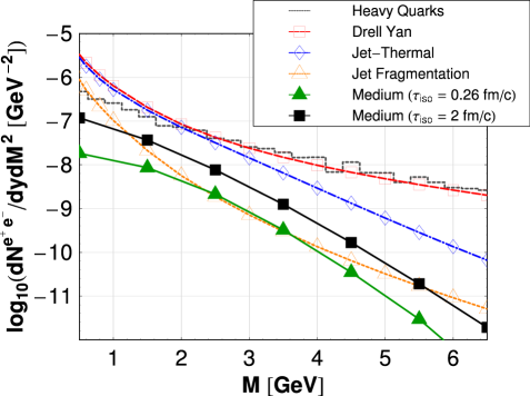
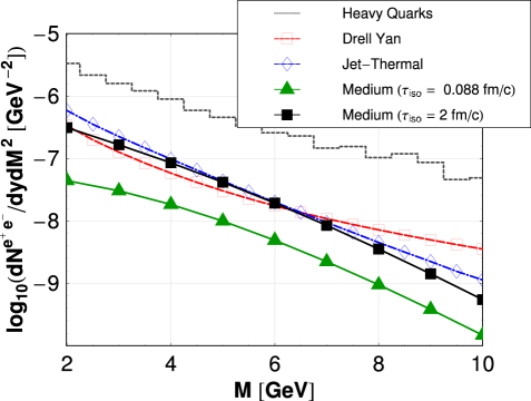
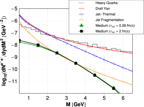
In Fig. 8, we show our predicted dilepton mass spectrum for RHIC and LHC energies assuming the time dependence of the energy density, the hard momentum scale and the anisotropy parameter are given by Eqns. (36) and (37) with . This corresponds to our free-streaming interpolating model. For us this model will serve as an upper-bound on the possible effect of momentum-space anisotropies on dilepton yields. From Fig. 8 we see that for both RHIC or LHC energies, there is a significant enhancement of up to one order of magnitude in the medium dilepton yield when we vary the isotropization time from to 2 fm/c. This enhancement is due to the fact that in 1+1 dimensional free streaming, the system preserves more transverse momentum as can be seen from Fig. 4. For fixed initial conditions this results in a larger effective temperature than would be obtained if the system underwent locally-isotropic (hydrodynamical) expansion throughout its evolution.
Nevertheless, as Fig. 8 shows, as a function of invariant mass, the other contributions to high-energy dilepton yields (Drell-Yan, jet-thermal, and jet-fragmentation) are all of the same order of magnitude as the medium contribution. This coupled with the large background coming from semileptonic heavy quarks decays would make it extremely difficult for experimentalists to extract a clean medium dilepton signal from the invariant mass spectrum. For this reason it does not look very promising to determine plasma initial conditions from the dilepton invariant mass spectrum. For this reason we will not present our predictions for the invariant mass spectrum for the intermediate models detailed below and only return to the invariant mass spectrum at the end of this section for completeness.
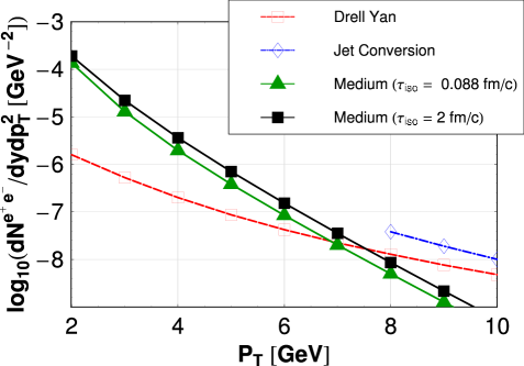
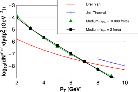
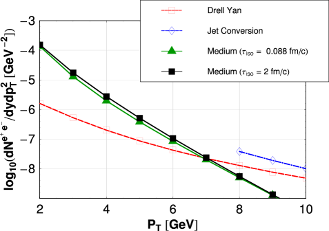
The good news is, however, that as a function of transverse momentum, see Fig. 9, the production of medium dileptons is expected to dominate other production mechanisms for 4 (6) GeV in the case of RHIC (LHC). In addition to this we see that for the free-streaming interpolating model that there is a significant enhancement of medium dileptons for both RHIC and LHC energies.
In order to quantify the effect of time-dependent pre-equilibrium emissions we define the “dilepton enhancement”, , as the ratio of the dilepton yield obtained with an isotropization time of to that obtained from an instantaneously thermalized plasma undergoing only 1+1 hydrodynamical expansion, ie. .
| (43) |
Using this criterion we find for the free streaming interpolating model with fixed initial conditions the dilepton enhancement at fm/c can be as large as 10. However, as mentioned above we expect that the actual enhancement will be lower due to the fact that parton interactions such as collisional-broadening will modify the free-streaming to something growing slower in proper time bringing the system closer to equilibrized expansion. In addition, as we will discuss below when using fixed initial conditions and there is significant entropy generation which, when properly normalized to fixed final multiplicity, results in reduced . Therefore, we expect obtained from the free streaming interpolation model with fixed initial conditions to be an upper-bound on the effect of pre-equilibrium emissions. Some of our results fixing initial conditions are related with recent work on dilepton production from a viscous QGP Dusling:2008xj .
IV.1.2 Collisionally-broadened interpolating model
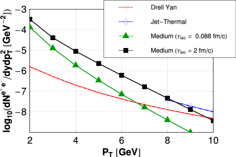
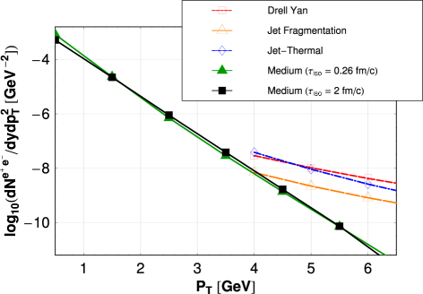
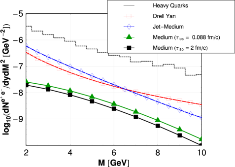
In Fig. 10, we show our predicted dilepton transverse momentum spectrum for RHIC and LHC energies assuming the time dependence of the energy density, the hard momentum scale and the anisotropy parameter are given by Eqns. (36) and (37) with . This corresponds to our collisionally-broadened interpolating model with fixed initial conditions. From Fig. 10 we see that for both RHIC or LHC energies, there is dilepton enhancement in the kinematic range shown; however, compared to the free streaming case the enhancement is reduced. This is due to the fact that the collisionally-broadened interpolating model is always closer to locally-isotropic expansion than the free-streaming () model, see Figs. 4 and 5.
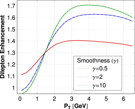
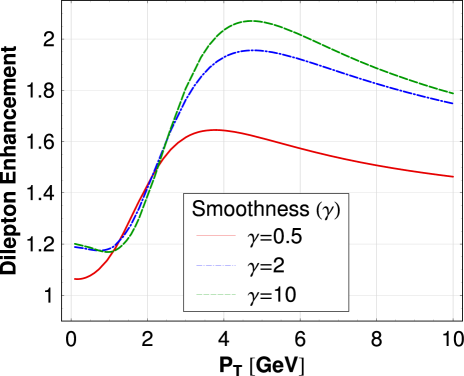
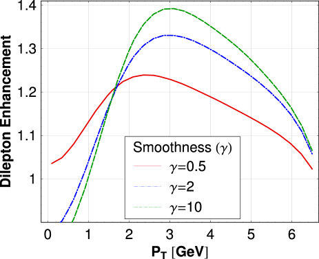
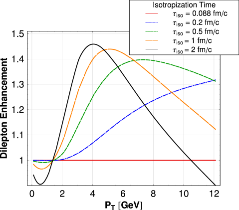
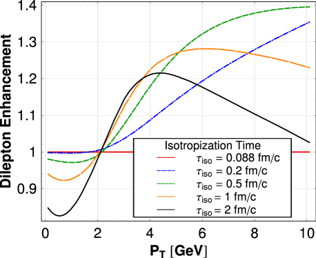
In Fig. 11 we show the dilepton enhancement, , as function of transverse momentum for fm/c at (left) RHIC energies (right) LHC energies. The invariant mass cut is the same as in Fig. 10 ( GeV). As can be seen from Fig. 11 using fixed initial conditions there is a rapid increase in between 1 and 3 GeV at RHIC energies and 1 and 4 GeV at LHC energies. The precise value of the enhancement depends on the assumed width and in Fig. 11 we show for . As can be seen from this figure both sharp and smooth transitions from early-time collisionally-broadened expansion to ideal hydrodynamic expansion result in a 40-70% enhancement of medium dilepton yields at RHIC energies and 60-100% at LHC energies. We will return to this in the results summary at the end of this section.
IV.2 Dilepton production with fixed final multiplicity
We now present the results of the dilepton production assuming the time dependence of the energy density, the hard momentum scale and the anisotropy parameter are given by Eqns. (36) and (42) with .
IV.2.1 Free streaming interpolating model
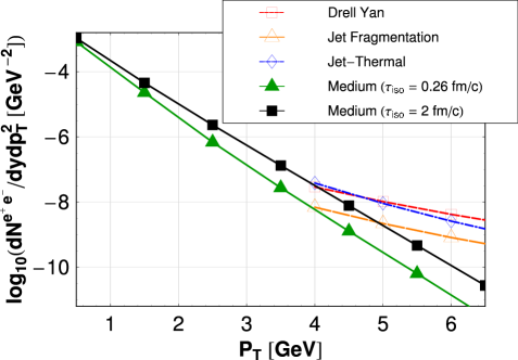
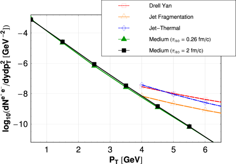
In Fig. 12, we show our predicted dilepton transverse momentum spectrum for RHIC and LHC energies assuming the time dependence of the energy density, the hard momentum scale and the anisotropy parameter are given by Eqns. (36) and (42) with . This corresponds to our free-streaming interpolating model with fixed final multiplicity. From Fig. 12 we see that for both RHIC or LHC energies, there is dilepton enhancement in the kinematic range shown; however, when fixing on final multiplicity the effect of a free-streaming pre-equilibrium phase is reduced. In fact, for small and large the free-streaming interpolating model with fixed final multiplicities predicts a suppression of dileptons. This is due to the fact that in order to maintain fixed final multiplicity for fm/c the free-streaming model initial energy density has to be reduced by (see top row of Fig. 7).
IV.2.2 Collisionally-broadened interpolating model
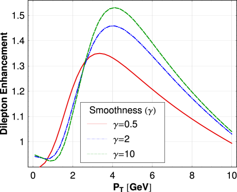
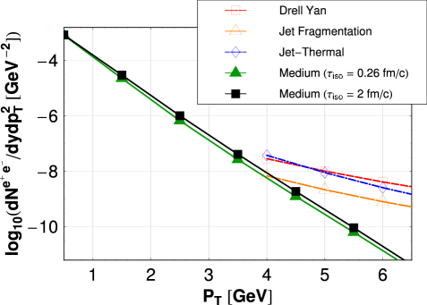
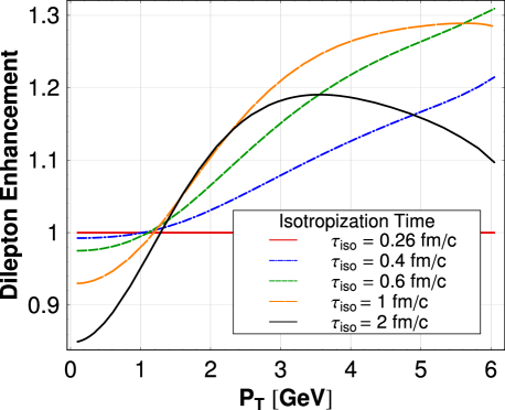
In Figs. 13 and 14, we show our predicted dilepton invariant mass and transverse momentum spectrum for RHIC and LHC energies assuming the time dependence of the energy density, the hard momentum scale and the anisotropy parameter are given by Eqns. (36) and (42) with . This corresponds to our collisionally-broadened interpolating model with fixed final multiplicity. In Fig. 15 we show the dilepton enhancement, , as function of transverse momentum for fm/c at (left) RHIC energies (right) LHC energies. The invariant mass cut is the same as in Fig. 14 ( GeV). As can be seen from Fig. 15 similar to the case of fixed initial conditions there is a rapid increase in between 1 and 3 GeV at RHIC energies and 1 and 4 GeV at LHC energies. However, compared to the case of the collisionally-broadened interpolating model with fixed initial condition (Fig. 11) the maximum enhancement is reduced slightly and we see a more pronounced peak in as a function of transverse momentum appearing. As can be seen from this figure both sharp and smooth transitions from early-time collisionally-broadened expansion to ideal hydrodynamic expansion result in a 20-40% enhancement of medium dilepton yields at RHIC energies, and 30-50% at LHC energies.
IV.3 Summary of Results
Based on the figures presented in the previous subsections we see that the best opportunity for measuring information about plasma initial conditions is from the GeV dilepton transverse momentum spectra between 1 6 GeV at RHIC and 2 8 GeV at LHC. This is due to the fact that medium dilepton yields dominate other mechanisms in that kinematic range and hence give the cleanest possible information about plasma initial conditions. In all cases shown above dilepton production is enhanced by pre-equilibrium emissions with the largest enhancements occurring when assuming fixed initial conditions and the free-streaming interpolating model. As we have mentioned above this model sets the upper-bound for the expected dilepton enhancement. Our most physically realistic model is the collisionally-broadened interpolating model with fixed final multiplicity so we will use it for our final predictions of expected dilepton enhancement. For this model, as can be seen from Fig. 15, assuming fm/c we find a 20-40% enhancement in dilepton yields at RHIC and 30-50% at LHC.
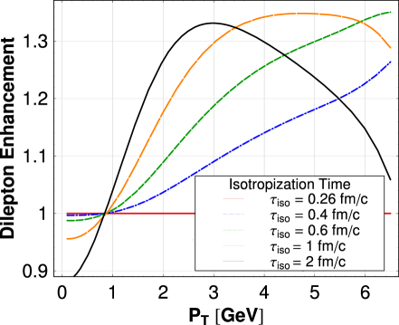
In addition we can calculate the dilepton enhancement for different assumed values for . This is shown for RHIC energies (left) and LHC energies (right) in Fig. 16 where we have fixed and varied to see the effect of varying the assumed isotropization time. As can be seen from this figure the effect of reducing is to shift the peak in to larger while at the same time reducing the overall amplitude of the peak. This feature seems generic at both RHIC and LHC energies. Therefore, in order to see the difference between an instantaneously thermalized QGP with and one with a later thermalization time requires determining the medium dilepton spectra between GeV at RHIC and GeV at LHC with high precision so that one could measure the less than 50% variation resulting from pre-equilibrium emissions.
Finally, we point out that in Fig. 16 we have chosen an invariant mass cut of GeV. Since our model predicts the full yields versus and it is possible to take other cuts (invariant mass and/or transverse momentum). This could be coupled with fits to experimental data, allowing one to fix and via a “multiresolution” analysis. To demonstrate the dependence of on the mass cut in Fig. 17 we show the dilepton enhancement, , using a mass cut of GeV. As can be seen from this Figure the qualitative features of our model’s predictions are similar to the lower mass cut presented in Fig. 16; however, for this mass cut we see that there is a stronger suppression of dilepton production at low and high invariant masses if there is late thermalization, fm/c. Such features can be used to constrain the model further when confronted with experimental data.
V Conclusions
In this work we have presented models which allow one to smoothly interpolate between early-time non-equilibrium 1+1 dimensional expansion to late-time isotropic equilibrium 1+1 dimensional hydrodynamic expansion. To accomplish this we introduced simple interpolating models with two parameters: , which is the time at which the system begins to expand hydrodynamically and which sets the width of the transition. Using these models we integrated the leading order rate for dilepton production in an anisotropic plasma over our modeled space-time evolution. Based on our numerical results for the variation of dilepton yields with the assumed values of we find that the best opportunity to determine information about the plasma isotropization time is by analyzing the high transverse momentum (1 6 GeV at RHIC and 2 8 GeV at LHC) dilepton spectra using relatively low pair invariant mass cuts ( GeV). Based on these spectra we introduced the “dilepton enhancement” factor which measures the ratio of yields obtained from a plasma which isotropizes at to one which isotropizes at the formation time, .
We showed that for our most extreme model, the free-streaming interpolating model () with fixed initial conditions, that the resulting enhancement can be as large as 10; however, this extreme model probably overestimates the amount of anisotropy in the plasma. Additionally, this model results in a large amount of entropy generation during the transition from the free-streaming asymptotic behavior to hydro asymptotic behavior. As we discussed this greatly constrains the maximum isotropization times which are consistent with experimental indications of low (10-20%) entropy generation.
In order to construct a more realistic model we then included collisional-broadening of the initial pre-equilibrium parton distribution functions (). In this more realistic model there is much less entropy generation and the system is always closer to ideal 1+1 hydrodynamic expansion than in the free-streaming interpolating model. As a result the dilepton enhancement due to pre-equilibrium emissions is lower than the free-streaming case. We find that when fixing final multiplicity at RHIC energies there is a 20-40% enhancement in the high-transverse momentum dileptons and at LHC energies it is 30-50% when one assumes an isotropization time of fm/c. The amplitude of the enhancement and position of the peak in the enhancement function, , varies with the assumed value of which, given sufficiently precise data, would provide a way to determine the plasma isotropization time experimentally. We presented our predictions for the dilepton enhancement, , as a function of for two different invariant mass cuts, demonstrating that our model can be constrained by a multiresolution analysis which should give higher statistics and further constrain the two model parameters at our disposal.
One shortcoming of this work is that we haven’t included NLO corrections to dilepton production from an anisotropic QGP. At low invariant mass these corrections would become important. As a next step one must undertake a calculation of the rate for dilepton pair production at NLO in an anisotropic plasma. This is complicated by the presence of plasma instabilities which render some expressions like correlators formally divergent and hence analytically meaningless. However, when combined with numerical solution of the long-time behavior of a plasma subject to the chromo-Weibel instability it may be possible to extract finite correlators ArnoldPersonal . This is a daunting but doable task. Absent such a calculation, phenomenologically speaking it is probably a very good approximation to simply take existing NLO calculations and apply the enhancement function as calculated at LO. We leave this for future work.
Another uncertainty comes from our implicit assumption of chemical equilibrium. If the system is not in chemical equilibrium (too many gluons and/or too few quarks) early time quark chemical potentials, or fugacities, will affect the production of lepton pairs Dumitru:1993vz ; Strickland:1994rf . However, to leading order the quark and gluon fugacities will cancel between numerator and denominator in the dilepton enhancement, Strickland:1994rf . We, therefore, expect that to good approximation one can factorize the effects of momentum space anisotropies and chemical non-equilibrium.
We note in closing that the interpolating model presented here has application beyond the realm of computing dilepton yields. In fact, such a model can be used to assess the phenomenological consequences of momentum-space anisotropies in other possible observables which are sensitive to early-time stages of the QGP, e.g., photon production Schenke:2006yp , heavy-quark transport, jet-medium induced electromagnetic radiation, etc.
Acknowledgements.
We thank to A. Dumitru, M. Gyulassy, A. Ipp, A. Rebhan, and B. Schenke for helpful discussions. We also thank S. Turbide for providing us predictions for the other relevant sources of dilepton production. M. Martinez gratefully acknowledges support by the Helmholtz Research School and Otto Stern School of the Johann Wolfgang Goethe-Universität. M.S. was supported by DFG project GR 1536/6-1.References
- (1) P. Huovinen, P. F. Kolb, U. W. Heinz, P. V. Ruuskanen and S. A. Voloshin, Phys. Lett. B 503 (2001) 58.
- (2) T. Hirano and K. Tsuda, Phys. Rev. C 66 (2002) 054905.
- (3) M. J. Tannenbaum, Rept. Prog. Phys. 69 (2006) 2005.
- (4) M. Luzum and P. Romatschke, Phys. Rev. C 78, 034915 (2008).
- (5) W. Jas and S. Mrowczynski, Phys. Rev. C 76, 044905 (2007).
- (6) R. Baier, A. H. Mueller, D. Schiff and D. T. Son, Phys. Lett. B 502 (2001) 51.
- (7) M. Strickland, J. Phys. G 34, S429 (2007).
- (8) S. Mrowczynski and M. H. Thoma, Phys. Rev. D 62 (2000) 036011.
- (9) J. Randrup and S. Mrowczynski, Phys. Rev. C 68 (2003) 034909.
- (10) P. Romatschke and M. Strickland, Phys. Rev. D 68 (2003) 036004.
- (11) P. Romatschke and M. Strickland, Phys. Rev. D 70, 116006 (2004).
- (12) P. Arnold, J. Lenaghan and G. D. Moore, JHEP 0308 (2003) 002.
- (13) S. Mrowczynski, A. Rebhan and M. Strickland, Phys. Rev. D 70 (2004) 025004.
- (14) P. Arnold, J. Lenaghan, G. D. Moore and L. G. Yaffe, Phys. Rev. Lett. 94 (2005) 072302.
- (15) A. Rebhan, P. Romatschke and M. Strickland, Phys. Rev. Lett. 94 (2005) 102303.
- (16) P. Arnold, G. D. Moore and L. G. Yaffe, Phys. Rev. D 72 (2005) 054003.
- (17) A. Rebhan, P. Romatschke and M. Strickland, JHEP 0509 (2005) 041.
- (18) P. Romatschke and R. Venugopalan, Phys. Rev. Lett. 96 (2006) 062302.
- (19) B. Schenke, M. Strickland, C. Greiner and M. H. Thoma, Phys. Rev. D 73 (2006) 125004.
- (20) B. Schenke and M. Strickland, Phys. Rev. D 74 (2006) 065004.
- (21) C. Manuel and S. Mrowczynski, Phys. Rev. D 74 (2006) 105003.
- (22) P. Romatschke and R. Venugopalan, Phys. Rev. D 74 (2006) 045011.
- (23) D. Bodeker and K. Rummukainen, JHEP 0707 (2007) 022.
- (24) P. Romatschke and A. Rebhan, Phys. Rev. Lett. 97 (2006) 252301.
- (25) A. Dumitru and Y. Nara, Phys. Lett. B 621 (2005) 89.
- (26) A. Dumitru, Y. Nara and M. Strickland, Phys. Rev. D 75 (2007) 025016.
- (27) A. Rebhan, M. Strickland and M. Attems, Phys. Rev. D 78, 045023 (2008).
- (28) C. Gale and K. L. Haglin, arXiv:hep-ph/0306098.
- (29) S. Turbide, “Electromagnetic radiation from matter under extreme conditions”, PhD Dissertation, UMI-NR-25272 (2006).
- (30) M. Martinez and M. Strickland, Phys. Rev. Lett. 100 (2008) 102301.
- (31) J. I. Kapusta, L. D. McLerran and D. Kumar Srivastava, Phys. Lett. B 283, 145 (1992).
- (32) A. Dumitru, D. H. Rischke, T. Schonfeld, L. Winckelmann, H. Stocker and W. Greiner, Phys. Rev. Lett. 70 (1993) 2860.
- (33) M. Strickland, Phys. Lett. B 331, 245 (1994).
- (34) J. Y. Ollitrault, Eur. J. Phys. 29 (2008) 275.
- (35) M. H. Thoma and C. T. Traxler, Phys. Rev. D 56 (1997) 198.
- (36) P. Arnold, G. D. Moore and L. G. Yaffe, JHEP 0206 (2002) 030.
- (37) F. Arleo et al., arXiv:hep-ph/0311131.
- (38) S. Turbide, C. Gale, D. K. Srivastava and R. J. Fries, Phys. Rev. C 74 (2006) 014903.
- (39) K. Kajantie, J. I. Kapusta, L. D. McLerran and A. Mekjian, Phys. Rev. D 34, 2746 (1986).
- (40) B. Kampfer and O. P. Pavlenko, Phys. Lett. B 289, 127 (1992).
- (41) J. D. Bjorken, Phys. Rev. D 27, 140 (1983).
- (42) G. Baym, Phys. Lett. B 138, 18 (1984).
- (43) K. Dusling and S. Lin, Nucl. Phys. A 809 (2008) 246.
- (44) D. Bodeker, JHEP 0510 (2005) 092.
- (45) P. Arnold and G. D. Moore, Phys. Rev. D 73 (2006) 025013.
- (46) P. Arnold and G. D. Moore, Phys. Rev. D 76 (2007) 045009.
- (47) A. Dumitru, E. Molnar and Y. Nara, Phys. Rev. C 76, 024910 (2007).
- (48) A. Ipp, personal communication.
- (49) P. Arnold, personal communication.
- (50) B. Schenke and M. Strickland, Phys. Rev. D 76, 025023 (2007).