Damping of forward neutrons in $pp$ collisions

Abstract

We calculate absorptive corrections to single pion exchange in the production of leading neutrons in $pp$ collisions. Contrary to the usual procedure of convolving the survival probability with the cross section, we apply corrections to the spin amplitudes. The non-flip amplitude turns out to be much more suppressed by absorption than the spin-flip one. We identify the projectile proton Fock state responsible for the absorptive corrections as a color octet-octet 5-quarks configuration. Calculations within two very different models, color-dipole light-cone description, and in hadronic representation, lead to rather similar absorptive corrections. We found a much stronger damping of leading neutrons than in some of previous estimates. Correspondingly, the cross section is considerably smaller than was measured at ISR. However, comparison with recent measurements by the ZEUS collaboration of neutron production in deep-inelastic scattering provides a strong motivation for challenging the normalization of the ISR data. This conjecture is also supported by preliminary data from the NA49 experiment for neutron production in $pp$ collisions at SPS.

I Introduction

The pion is known to have a large coupling to nucleons, therefore pion exchange is important in processes with isospin one in the cross channel (e.g. $p+n\to n+p$). However, the pion Regge trajectory has a low intercept $\alpha_{\pi}(0)\approx 0$, and this is why it ceases to be important at high energies in binary reactions, while other mesons, $\rho,\ a_{2}$, etc. take over.

Quite a different situation occurs in inclusive reactions of leading neutron production. Inclusive reactions in general are known to have (approximate) Feynman scaling, and as a consequence the pion contribution to neutron production remains nearly unchanged with energy. This can be seen from the graphical representation of the cross section of the inclusive reaction $h+p\to X+n$, depicted in Fig. 1.

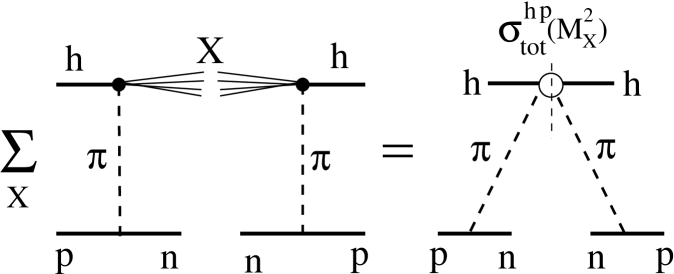
Figure 1: Graphical representation of the cross section of inclusive neutron production in hadron-proton collisions, in the fragmentation region of the proton.

Summing up all final states $X$ at a fixed invariant mass $M_{X}$ and relying on the optical theorem, one arrives at the total hadron-pion cross section at c.m. energy $M_{X}$. This cross section is a slowly varying function of $M_{X}$ (restricted by the Froissart bound), and this is the source for Feynman scaling. At the same time, the effective interval of energy squared for pion exchange is less than $s$, which is the c.m. energy squared for $hp$ collisions. Indeed, the effective energy squared interval $s^{\prime}$ is given by the multi-peripheral kinematics of particle production as,

$${s^{\prime}\over s_{0}}={s\over M_{X}^{2}}\approx{1\over 1-z}\,,$$ (1)

where $s_{0}$ is the scale factor, usually fixed at $1\,\mbox{GeV}^{2}$; and $z=p_{n}^{+}/p_{p}^{+}$ is the fraction of the proton light-cone momentum carried by the neutron, which is close to Feynman $x_{F}$ at large $z\to 1$.

In fact, the pion exchange brings in a factor $(1-z)^{-2\alpha_{\pi}}$ ($\alpha_{\pi}(t)$ is the pion Regge trajectory) to the cross section, which is independent of the collision energy $s$, if $z$ is fixed. Thus, the pion exchange contribution does not vanish with energy, and this is in more detail the origin of the Feynman scaling. From the point of view of dispersion relations, the smaller the 4-momentum transfer squared $t$, the closer we approach the pion pole, and the more important is its contribution. The smallest values of $t$ are reached in the forward direction and at $z\to 1$. The latter condition, however, leads to the dominance of other Reggeons which have higher intercepts. Indeed, the corresponding Regge factor $(1-z)^{-2\alpha_{\footnotesize{I\!\!R}}}$ for $\rho$ and $a_{2}$ Reggeons is about $1/(1-z)$ times larger than the one for pion. Although in general these Reggeons are suppressed by an order of magnitude compared to the pion k2p , they become equally important and start taking over at $z\mathrel{\hbox to0.0pt{\lower 4.0pt\hbox{\hskip 1.0pt$\sim$}\hss}\raise 1.0pt\hbox{$>$}}0.9$.

Another important correction, which is the main focus of this paper, is the effect of absorption, or initial/final state interactions. The active projectile partons participating in the reaction, as well as the spectator ones, can interact with the proton target or with the recoil neutron, and initiate particle production, which usually leads to a substantial reduction of the neutron momentum. The probability that this does not happen, called sometimes survival probability of a large rapidity gap, leads to a suppression of leading neutrons produced at large $z$. There are controversies regarding the magnitude of this suppression. Some calculations predict quite a mild effect, of about $10\%$ boreskov1 ; boreskov2 ; 3n ; ap , while others strong1 ; strong2 ; ryskin expect a strong reduction by about a factor of 2. See ryskin for a discussion of the current controversies in data and theory, for leading neutron production.

Usually absorptive corrections are calculated in a probabilistic way, convolving the gap survival probability with the cross section. We found, however, that the spin amplitudes of neutron production acquire quite different suppression factors, and one should work with amplitudes, rather than with probabilities.

In Sect. II we introduce the spin amplitudes for inclusive production of neutrons and calculate the cross section in Born approximation of single pion exchange. Contrary to the usual case in binary reactions, the spin non-flip term is large and rises towards small $z$. Comparison with ISR measurements isr shows that the calculation overshoots somewhat the data, albeit only by about $10\%$. Calculations also result in a substantial rise of the cross section with energy.

In Sect. III the absorptive corrections are introduced. Assuming that the corrections factorize in impact parameter space, the spin amplitudes are transformed to this representation, and the general expression for the gap survival amplitude is derived. We found that the main Fock component of the incoming proton, which is responsible for the absorptive corrections, is a 5-quark color octet-octet state. Therefore it is not a surprise that the resulting neutron damping at which we arrive is quite strong. In order to figure out what was missed in previous calculations which led to a weak absorption damping, in Sect. III.3 we reformulated the current mechanism in terms of Reggeon calculus.

We calculate the gap survival amplitude within two quite different models. In Sect. IV we employ the well developed phenomenology of light-cone color dipoles fitted to photoproduction and deep-inelastic scattering (DIS) data. We use the saturated model for the dipole cross section, generalized recently to a partial dipole-proton amplitude.

Another model for the survival amplitude is presented in Sect. V. Expanding the 5-quark Fock state over the full set of hadronic states, we assumed that the $\pi p$ pair containing the 5 valence quark is the dominant term. The gap survival amplitudes of pion and proton was extracted in a model independent way directly from data for elastic $\pi p$ and $pp$ scattering. We found that the results of the two models, based on dipole and hadronic representations, resulted in rather similar gap survival amplitudes.

In Sect. VI we calculate the spin non-flip and flip contributions to the cross section, and found that the inclusive cross section of neutron production is about twice as small as the original result of the Born approximation. We also conclude that absorptive corrections practically terminate the strong energy dependence that results from the Born approximation. The ISR data support this observation.

Although the calculated shape of $z$-distribution is improved by absorption and corresponds to the shape of the ISR data at $q_{T}=0$, the overall normalization is quite lower than in the data. In Sect. VII.2 we compare the ISR data with other measurements, in particular with the recent results of the ZEUS collaboration for inclusive neutron production in the photoabsorption reaction $\gamma p\to Xn$. The two sets of data turn out to be not really consistent, what makes questionable the normalization of the ISR data.

We summarize the main results and observations in Sect. VIII.

II Pion pole

The Born approximation pion exchange contribution to the amplitude of neutron production $pp\to nX$, depicted in Fig. 2a, in the leading order in small parameter $m_{N}/\sqrt{s}$ has the form

$$A^{B}_{p\to n}(\vec{q},z)=\frac{1}{\sqrt{z}}\,\bar{\xi}_{n}\left[\sigma_{3}\,\tilde{q}_{L}+\vec{\sigma}\cdot\vec{q}_{T}\right]\xi_{p}\,\phi^{B}(q_{T},z)\,,$$ (2)

where $\vec{\sigma}$ are Pauli matrices; $\xi_{p,n}$ are the proton or neutron spinors; $\vec{q}_{T}$ is the transverse component of the momentum transfer;

$$\tilde{q}_{L}=(1-z)\,m_{N}\,.$$ (3)

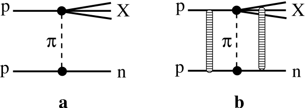
Figure 2: a: Born graph with single pion exchange; b: illustration of absorptive corrections.

In the region of small $1-z\ll 1$ the pseudoscalar amplitude $\phi^{B}(q_{T},z)$ has the triple-Regge form,

$$\phi^{B}(q_{T},z) = \frac{\alpha_{\pi}^{\prime}}{8}\,G_{\pi^{+}pn}(t)\,\eta_{\pi}(t)\,(1-z)^{-\alpha_{\pi}(t)}$$ (4)

$$\times A_{\pi^{+}p\to X}(M_{X}^{2})\,,$$

where the 4-momentum transfer squared $t$ has the form,

$$t=-\,{1\over z}\,\left(\tilde{q}_{L}^{2}+q_{T}^{2}\right)\,,$$ (5)

and $\eta_{\pi}(t)$ is the phase (signature) factor which can be expanded near the pion pole as,

$$\eta_{\pi}(t)=i-ctg\left[\frac{\pi\alpha_{\pi}(t)}{2}\right]\approx i+\frac{2}{\pi\alpha_{\pi}^{\prime}}\,\frac{1}{m_{\pi}^{2}-t}\,.$$ (6)

We assume a linear pion Regge trajectory $\alpha_{\pi}(t)=\alpha_{\pi}^{\prime}(t-m_{\pi}^{2})$, where $\alpha_{\pi}^{\prime}\approx 0.9\,\mbox{GeV}^{-2}$. The imaginary part in (6) is neglected in what follows, since its contribution near the pion pole is small.

The effective vertex function $G_{\pi^{+}pn}(t)=g_{\pi^{+}pn}\exp(R_{1}^{2}t)$ includes the pion-nucleon coupling and the form factor which incorporates the $t$-dependence of the coupling and of the $\pi N$ inelastic amplitude. We take the values of the parameters used in k2p , $g^{2}_{\pi^{+}pn}(t)/8\pi=13.85$ and $R_{1}^{2}=0.3\,\mbox{GeV}^{-2}$. Notice that the choice of $R_{1}$ does not bring much uncertainty, since we focus here at data for forward production, $q_{T}=0$, so $t$ is quite small.

The amplitudes in (2)-(4) are normalized as,

$$\sigma^{\pi^{+}p}_{tot}(s^{\prime}=M_{X}^{2})={1\over M_{X}^{2}}\sum\limits_{X}|A_{\pi^{+}p\to X}(M_{X}^{2})|^{2}\,,$$ (7)

where different hadronic final states $X$ are summed at fixed invariant mass $M_{X}$. Correspondingly, the differential cross section of inclusive neutron production reads bishari ; 2klp ,

$$z\,\frac{d\sigma^{B}_{p\to n}}{dz\,dq_{T}^{2}} = {1\over s}\left|A^{B}_{p\to n}(\vec{q}_{T},z)\right|^{2}$$ (8)

$$= \left(\frac{\alpha_{\pi}^{\prime}}{8}\right)^{2}|t|G_{\pi^{+}pn}^{2}(t)\left|\eta_{\pi}(t)\right|^{2}(1-z)^{1-2\alpha_{\pi}(t)}$$

$$\times \sigma^{\pi^{+}p}_{tot}(s^{\prime}=M_{X}^{2})\,.$$

Since at $z\to 1$ the value of $M_{X}^{2}$ decreases, we rely on a realistic fit to the experimental data pdg for $\pi^{+}p$ total cross section.

The results of the Born approximation calculation, Eq. (8), at $\sqrt{s}=200,\ 62.7$ and $30.6\,\mbox{GeV}$, are depicted together with the ISR data isr , in Figs. 3 and 4.

Figure 3: Born approximation (dashed curve) for leading neutron production and ISR data isr , at $\sqrt{s}=62.7\,\mbox{GeV}$ and $p_{T}=0$. Two solid curves, the upper and bottom ones, show the effect of absorptive corrections calculated in the dipole approach ($\times S^{(5q)}$) and in hadronic representation ($\times S^{(hadr)}$) respectively.

Figure 4: Energy dependence of inclusive neutron production. The three upper curves present the forward cross section at $\sqrt{s}=30.6\,\mbox{GeV}$ (solid), $62.7\,\mbox{GeV}$ (dashed) and $200\,\mbox{GeV}$ (dotted-dashed), calculated in the Born approximation. The same cross sections, although corrected for absorption ($\times S^{(5q)}$), are given by the three curves at the bottom. Data at $\sqrt{s}=30.6\,\mbox{GeV}$ and $62.7\,\mbox{GeV}$ isr are depicted by squares and inverse triangles respectively

The data are given at two energies $\sqrt{s}=30.6\,\mbox{GeV}$ and $62.7\,\mbox{GeV}$, and therefore we use these energies in our calculations. One can see that the Born approximation considerably exceeds the data.

Notice that only at small $1-z\sim m_{\pi}/m_{N}$ one can approach the pion pole, i.e. the smallness of the pion mass is important for Eq. (4). Otherwise $t$ is large even at $q_{T}=0$, and the pion exchange gains a considerable imaginary part. Besides, the spin-flip amplitude $\phi^{B}(q_{T},z)$ acquires a weak dependence on $q_{T}$ at small scattering angles, $q_{T}^{2}\ll(1-z)^{2}m_{N}^{2}$.

III Absorptive corrections

Absorptive corrections, or initial/final state interactions, illustrated in Fig. 2, look quite complicated in momentum representation where they require multi-loop integrations. However, if they do not correlate with the amplitude of the process $\pi^{+}p\to X$, then these corrections factorize in impact parameter and become much simpler. Therefore, first of all, we should Fourier transform the amplitude Eq. (2) to impact parameter space.

III.1 Impact parameter representation

The partial Born amplitude at impact parameter $\vec{b}$, corresponding to (2), has the form,

$$f^{B}_{p\to n}(\vec{b},z)=\frac{1}{\sqrt{z}}\,\bar{\xi}_{n}\left[\sigma_{3}\,\tilde{q}_{L}\,\theta^{B}_{0}(b,z)-i\,\frac{\vec{\sigma}\cdot\vec{b}}{b}\,\theta^{B}_{s}(b,z)\right]\xi_{p}\,,$$ (9)

where

$$\theta^{B}_{0}(b,z) = \int d^{2}q\,e^{i\vec{b}\vec{q}}\,\phi^{B}(q_{T},z)$$ (10)

$$= \frac{N(z)}{1-\beta^{2}\epsilon^{2}}\,\left[K_{0}(\epsilon b)-K_{0}(b/\beta)\right]\,;$$

$$\theta^{B}_{s}(b,z) = {1\over b}\int d^{2}q\,e^{i\vec{b}\vec{q}}\,(\vec{b}\cdot\vec{q})\,\phi^{B}(q_{T},z)$$ (11)

$$= \frac{N(z)}{1-\beta^{2}\epsilon^{2}}\,\left[\epsilon\,K_{1}(\epsilon b)-\frac{1}{\beta}\,K_{1}(b/\beta)\right]\,.$$

Here

$$N(z) = \frac{1}{2}\,g_{\pi^{+}pn}\,z(1-z)^{\alpha^{\prime}_{\pi}(m_{\pi}^{2}+\tilde{q}_{L}^{2}/z)}e^{-R_{1}^{2}\tilde{q}_{L}^{2}/z}$$

$$\times A_{\pi p\to X}(M_{X}^{2})\,$$

$$\epsilon^{2} = \tilde{q}_{L}^{2}+zm_{\pi}^{2}\,,$$

$$\beta^{2} = R_{1}^{2}-\alpha_{\pi}^{\prime}\,\frac{\ln(1-z)}{z}\,.$$ (12)

To simplify the calculations we replaced here the Gaussian form factor, $\exp(-\beta^{2}q_{T}^{2})$, by the monopole form $1/(1+\beta^{2}q_{T}^{2})$, which is a good approximation at the small values of $q_{T}$ we are interested in. At the same time we keep the exact expression for the dependence on $\tilde{q}_{L}$, which can be rather large.

III.2 Survival amplitude of large rapidity gaps

At large $z\to 1$ the process under consideration is associated with the creation of a large rapidity gap (LRG), $\Delta y=|\ln(1-z)|$, where no particle is produced. Absorptive corrections may also be interpreted as a suppression related to the survival probability of LRG, which otherwise can be easily filled by multiparticle production initiated by inelastic interactions of the projectile partons with the target. Usually the corrected cross section is calculated as a convolution of the cross section with the survival probability factor (see ryskin and references therein). This recipe may work sometimes as an approximation, but only for $q_{T}$-integrated cross section. Otherwise one should rely on a survival amplitude, rather than probability. Besides, the absorptive corrections should be calculated differently for the spin-flip and non-flip amplitudes (see below).

In impact parameter representation one can expand the incoming proton over the Fock components, $|3q\rangle,\ |3qg\rangle,\ |4q\bar{q}\rangle$, etc. For every Fock state with fixed transverse separations between the constituents the eikonal form is exact. In the dipole representation the absorption corrected amplitude can be written as,

$$f_{p\to n}(b,z) = \sum\limits_{l}\prod\limits_{i}d^{2}r_{i}\,d\alpha_{i}\,C^{p}_{l}(\{r_{i},\alpha_{i}\})\,$$ (13)

$$\times \left[\tilde{f}^{B}_{p\to n}(b,z,\{r_{i},\alpha_{i}\})\right]_{l}e^{if_{l}(b,z,\{r_{i}\})}.$$

Here we sum over Fock states containing different number of partons of different species, having transverse positions $\vec{r}_{i}$ and fractional light-cone momenta $\alpha_{i}$. The parton distribution amplitudes $C^{p}_{l}(\{r_{i},\alpha_{i}\})$ are normalized to the probabilities $W_{l}$ of having $l$-th Fock state in the proton, $\int\prod\limits_{i}d^{2}r_{i}\,d\alpha_{i}|C^{p}_{l}(\{r_{i},\alpha_{i}\})|^{2}=W_{l}$. We neglect the small real part of the partial amplitude $f_{l}(b,z,\{r_{i}\})$ of elastic scattering of the partonic state $|l;\{r_{i}\}\rangle$ on a nucleon, and assume that it is pure imaginary and isotopic invariant (Pomeron exchange).

Now we have to identify the Fock states responsible for initial and final state interactions leading to absorptive corrections. We start with Fig. 5a, containing the amplitude of the pion-proton inelastic collision $\pi+p\to X$. This is usually described as color exchange, leading to the creation of two color octet states with a large rapidity interval $\sim\ln(M_{X}^{2}/s_{0})$ ($s_{0}=1\,\mbox{GeV}^{2}$), as illustrated in Fig. 5b.

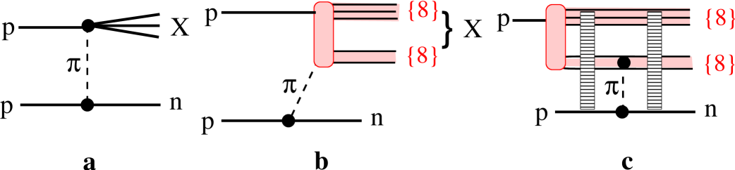
Figure 5: a: Born graph with single pion exchange and excitation of the projectile proton, $p+\pi\to X$; b: inelastic proton-pion interaction, $p+\pi\to X$, via color exchange, leading to the production of two color-octet dipoles which hadronize further to $X$; c: Fock state representation of the previous mechanism. A color octet-octet dipole which is a 5-quark Fock component of the projectile proton, interacts with the target proton via $\pi^{+}$ exchange. This 5-quark state may experience initial and final state interaction via vacuum quantum number (Pomeron) exchange with the nucleons (ladder-like strips).

Perturbatively, the interaction is mediated by gluonic exchanges. Nonperturbatively, e.g. in the string model, the hadron collision looks like intersection and flip of strings. Hadronization of the color-octet dipole (described for example by the string model) leads to the production of different final states $X$.

According to Fig. 5b the produced color octet-octet state can experience final state interactions with the recoil neutron. On the other hand, at high energies multiple interactions become coherent, and one cannot specify at which point the charge-exchange interaction happens, i.e. both initial and final state interactions must be included. One can rephrase this in terms of the Fock state decomposition. The projectile proton can fluctuate into a 5-quark color octet-octet before the interaction with the target. The fluctuation life-time, or coherence time (length), is given by

$$l_{c}=\frac{2E_{p}}{M_{X}^{2}-m_{N}^{2}}\,,$$ (14)

which rises with energy and at high energies considerably exceeds the longitudinal size of target proton. Technically, one should integrate the amplitude over the longitudinal coordinate $l$ of the fluctuation point, weighted with a phase factor $e^{il/l_{c}}$ (see an example in kst2 ), which effectively restricts the distances from the target to $\Delta l\mathrel{\hbox to0.0pt{\lower 4.0pt\hbox{\hskip 1.0pt$\sim$}\hss}\raise 1.0pt\hbox{$<$}}l_{c}$.

This leads to a different space-time picture of the process at high energies, namely the incoming proton fluctuates into a 5-quark state $|\{3q\}_{8}\{\bar{q}q\}_{8}\rangle$ long in advance of the interaction between the $\{\bar{q}q\}_{8}$ pair and the target via pion exchange, see Fig. 5c. This is the general intuitive picture which is supported by more formal calculations zamolodchikov ; stan-ivan . Assuming only final state interactions one should sum up the amplitudes of the process depicted in Fig. 5b and of the double step collision in which the 5-quark state is produced diffractively in the first collision $pN\to|\{3q\}_{8}\{\bar{q}q\}_{8}\rangle\,N$, and then the 5-quark system experiences charge exchange scattering of another proton via pion exchange. The resulting amplitude exposes both initial and final state attenuation of the 5-quark state,

$$f_{p\to n}(b,z)=f^{B}_{p\to n}(b,z)\,S^{(}b,z)\,.$$ (15)

Thus, the 5-quark component of the projectile proton propagates through the target experiencing initial and final state interactions. The effective absorption cross section is the inelastic cross section of the $|\{3q\}_{8}\{\bar{q}q\}_{8}\rangle$ dipole on a nucleon.

Of course, besides the five valence quarks, also gluons can be radiated, which are essential for the energy dependence of $\sigma^{\pi p}_{tot}(M_{X}^{2})$. They are effectively included in the following calculations.

III.3 Reggeon calculus

Previous calculations 3n ; ryskin proposed rather mild absorptive corrections, corresponding to only a beam proton experiencing multiple interactions in the target. This was motivated by Reggeon graphs depicted in Fig. 6a,b (we show only some of the interference terms))

Figure 6: Absorptive corrections due to possibility of inelastic interactions which can fill up the large rapidity gap. a: Interactions of the projectile proton and its remnants (see Fig. 7) with the target ; b: triple Pomeron interaction due to interactions of produced particles (e.g. radiated gluons); c: interactions including the pion remnants (see Fig. 7). Only some of the interference graphs are shown.

Fig. 6a presents multiple interactions of the projectile proton and its remnants. Fig. 6b includes interactions of the multiparton states produced in $\pi-p$ inelastic collision (see Fig. 2). This term is proportional to the triple-Pomeron coupling, which is assumed to be small, and for this reason it was neglected in 3n ; ap ; ryskin . The third term Fig. 6c, overlooked in 3n ; ap , has a different behavior since it contains a 4-Reggeon vertex $\pi\pi{I\!\!P}{I\!\!P}$, and may not be small. The structure of this vertex, as well as of the cut Pomeron, are shown in Fig. 7.

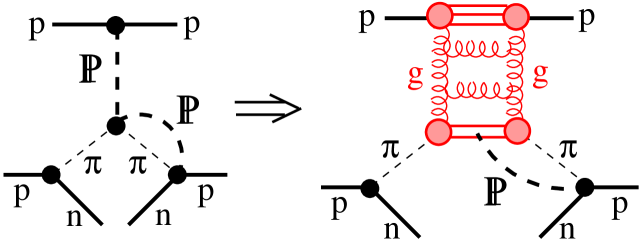
Figure 7: Structure of the four-Reggeon vertex $\pi\pi{I\!\!P}{I\!\!P}$.

The interaction of the radiated gluons (the rungs of the Pomeron ladder) is indeed weak, as follows from the smallness of the triple-Pomeron coupling. This is explained dynamically in spots by the shortness of the transverse separation between the radiated gluons and the source. There is no such a suppression, however, for the interaction of the ${\bar{q}q}_{8}$ pair, which is the pion remnant, as is depicted in Fig. 7. Calculations performed below confirm that the term shown in Figs. 6c, 7, missed in 3n ; ryskin , is large.

IV Absorptive corrections in saturated regime

Another way to estimate the absorption effects is to consider directly the interaction of the 5-quark octet-octet dipole with the proton target. Following the dual parton model capella approach, we replace the $|3q\rangle_{8}-|\bar{q}q\rangle_{8}$ dipole by two color triplet dipoles, $(qq)-q$ and $q-\bar{q}$, as is illustrated in Fig. 8.

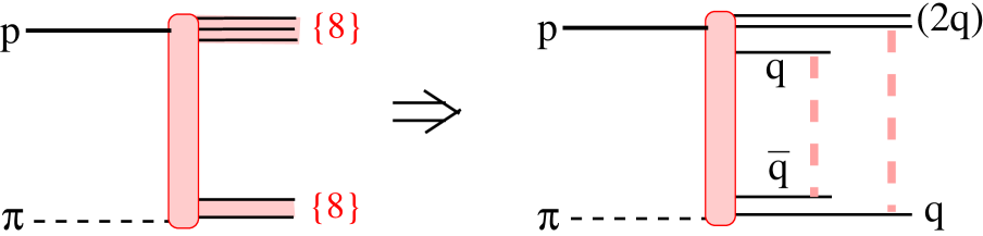
Figure 8: Inelastic pion-proton interaction, $\pi+p\to X$, in Fig. 5, leading to the production of two color-triplet dipoles, $q-\bar{q}$ and $(2q)-q$.

This approximation has an accuracy $1/N_{c}^{2}$, which is sufficient for our purposes.

Thus, the survival amplitude for such a 5-quark state can be represented as a product,

$$S^{(5q)}(b) = S^{(3q)}(b)\,S^{(q\bar{q})}(b)$$

$$= \left[1-\,{\rm Im}\,\Gamma^{(3q)p}(b)\right]\left[1-\,{\rm Im}\,\Gamma^{(\bar{q}q)p}(b)\right].$$

similar to Eq. (34), The elastic amplitude $\Gamma^{(\bar{3}3)p}(b)$ of a color $\{\bar{3}3\}$ dipole interacting with a proton is related to the partial elastic amplitude

$$\,{\rm Im}\,\Gamma^{(\bar{3}3)p}(b,z)=\int d^{2}rW_{\bar{3}3}(r,M_{X}^{2})\,\,{\rm Im}\,f^{\bar{3}3}_{el}(\vec{b},\vec{r},s,\alpha),$$ (17)

where $\alpha$ is the fractional light-cone momentum carried by the $3$, or $\bar{3}$; $r$ is the dipole transverse size; and $W_{\bar{3}3}(r,M_{X}^{2})$ is the dipole size distribution function, which is specified later, as well as the relation between $\alpha$ and $z$. Now we concentrate on the partial dipole amplitude $f^{\bar{3}3}_{el}(\vec{b},\vec{r},s,\alpha)$.

IV.1 Generalized unintegrated gluon density and partial dipole amplitude

The $\bar{q}q$-dipole-proton total cross section can be directly fitted to data on the proton structure function measured in deep-inelastic scattering (DIS). The popular form gbw of the dipole cross section, which describes quite well data at small Bjorken $x$, has a saturated shape, i.e. the cross section levels off at large dipole sizes. For soft reactions, such as the one we are dealing with here, the c.m. energy rather than Bjorken $x$, is the proper variable. A similar parameterization, with the saturated shape fitted to data on DIS at $Q^{2}$ not high and real photo-absorption and photoproduction of vector mesons, led to the result kst2 ,

$$\sigma_{\bar{q}q}(r,s)=\sigma_{0}(s)\left[1-e^{-r^{2}/R_{0}^{2}(s)}\right]\,,$$ (18)

where $R_{0}(s)=0.88\,fm\,(s_{0}/s)^{0.14}$ and $s_{0}=1000\,GeV^{2}$. This cross section is normalized to reproduce the pion-proton total cross section, $\int d^{2}r\,|\Psi_{\pi}(r)|^{2}\sigma_{\bar{q}q}(r,s)=\sigma^{\pi p}_{tot}(s)$. The pion wave function squared integrated over longitudinal quark momenta has the form,

$$\left|\Psi_{\pi}(\vec{r})\right|^{2}=\frac{3}{8\pi\langle r^{2}_{ch}\rangle_{\pi}}\exp\left(-\frac{3r^{2}}{8\langle r^{2}_{ch}\rangle_{\pi}}\right)\,,$$ (19)

where $\langle r^{2}_{ch}\rangle_{\pi}=0.44\,\mbox{fm}^{2}$ r-pion is the mean pion charge radius squared. This normalization condition results in

$$\sigma_{0}(s)=\sigma^{\pi p}_{tot}(s)\,\left(1+\frac{3\,R^{2}_{0}(s)}{8\,\langle r^{2}_{ch}\rangle_{\pi}}\right)\,,$$ (20)

For the numerical calculation we rely on one of the popular parameterizations for the energy dependent total cross sections pdg (only the Pomeron part), $\sigma^{\pi p}_{tot}(s)=\Sigma_{0}+\Sigma_{1}\ln^{2}(s/s_{1})$, where $\Sigma_{0}=20.9\,\mbox{mb}$ $\Sigma_{1}=0.31\,\mbox{mb}$ and $s_{1}=28.9\,\mbox{GeV}^{2}$.

Just as the dipole-proton total cross section can be calculated via the unintegrated gluon density in the proton gbw , one can calculate the partial amplitude $f(\vec{b},\vec{r})$ via a generalized transversely off-diagonal gluon distribution amir2 ,

$${\rm Im}f^{N}_{\bar{q}q}(\vec{b},\vec{r},\beta) = \frac{1}{12\pi}\int\frac{d^{2}q\,d^{2}q^{\prime}}{q^{2}\,q^{\prime 2}}\,\alpha_{s}\,{\cal F}(x,\vec{q},\vec{q}^{\,\prime})e^{i\vec{b}\cdot(\vec{q}-\vec{q}^{\,\prime})}$$ (21)

$$\times \left(e^{-i\vec{q}\cdot\vec{r}\beta}-e^{i\vec{q}\cdot\vec{r}(1-\beta)}\right)\,$$

$$\times \left(e^{i\vec{q}^{\,\prime}\cdot\vec{r}\beta}-e^{-i\vec{q}^{\,\prime}\cdot\vec{r}(1-\beta)}\right)\,\,.$$

A model for the generalized unintegrated gluon density was proposed recently amir2 , based on the saturated form of the diagonal gluon density gbw , and assuming a factorized dependence on both $\vec{q}$ and $\vec{q}^{\,\prime}$. One gets

$${\cal F}(x,\vec{q},\vec{q}^{\ \prime})=\frac{3\,\sigma_{0}}{16\,\pi^{2}\,\alpha_{s}}\ q^{2}\,q^{\prime\,2}\,R_{0}^{2}(x)$$

$$\times {\rm exp}\Bigl{[}-{1\over 8}\,R_{0}^{2}(x)\,(q^{2}+q^{\prime\,2})\Bigr{]}{\rm exp}\bigl{[}-{1\over 2}B(x)(\vec{q}-\vec{q}^{\ \prime})^{2}\bigr{]}\,,$$

This Bjorken $x$-dependent density, appropriate for hard reactions, leads to an $x$-dependent partial amplitude amir2 . Although in general it should not be used for soft processes, one can switch from an $x$- to an $s$-dependence keeping the same parameterization and adjusting the parameters to observables in soft reactions, as was done in kst2 , see Eq. (18). Then the partial amplitude reads

$$\,{\rm Im}\,f^{\bar{q}q}_{el}(\vec{b},\vec{r},s,\alpha)=\frac{\sigma_{0}(s)}{8\pi B(s)}\,\Biggl{\{}\exp\left[-\frac{[\vec{b}+\vec{r}(1-\alpha)]^{2}}{2B(s)}\right]+\exp\left[-\frac{(\vec{b}-\vec{r}\alpha)^{2}}{2B(s)}\right]-2\exp\Biggl{[}-\frac{r^{2}}{R_{0}^{2}(s)}-\frac{[\vec{b}+(1/2-\alpha)\vec{r}]^{2}}{2B(s)}\Biggr{]}\Biggr{\}},$$

(23)

This partial amplitude correctly reproduces the dipole cross section Eq. (18),

$$2\int d^{2}b\,{\rm Im}f^{\bar{q}q}_{el}(\vec{b},\vec{r},s,\alpha)=\sigma_{\bar{q}q}(r,s)\,.$$ (24)

Another condition that needs to be satisfied is reproducing the slope $B^{\pi p}_{el}(s)$ of the elastic $\pi p$ differential cross section,

$$B^{\pi p}_{el}(s) = {1\over 2}\,\langle b^{2}\rangle\frac{1}{\sigma^{\pi p}_{tot}}\int d^{2}b\int\limits_{0}^{1}d\alpha$$ (25)

$$\times \int d^{2}r\,\left|\Psi_{\pi}(\vec{r},\alpha)\right|^{2}{\rm Im}f^{\bar{q}q}_{el}(\vec{b},\vec{r},s,\alpha)\,.$$

This condition allows to evaluate the parameter $B(s)$ in (23). To simplify this calculation, we fix here $\alpha=1/2$ in the partial amplitude and arrive at

$$B(s)=B^{\pi p}_{el}(s)-{1\over 3}\,\langle r_{ch}^{2}\rangle_{\pi}-{1\over 8}\,R_{0}^{2}(s)\,.$$ (26)

In what follows we use a Regge parameterization for the elastic slope, $B^{\pi p}_{el}(s)=B_{0}+2\alpha_{I\!\!P}^{\prime}\ln(s/\mu^{2})$, with $B_{0}=6\,\mbox{GeV}^{-2}$, $\alpha_{I\!\!P}^{\prime}=0.25\,\mbox{GeV}^{-2}$, and $\mu^{2}=1\,\mbox{GeV}^{2}$.

In the case of a $(2q)-q$ dipole all relations are analogous to Eqs. (18)-(26), but one should make the following replacements: (i) $\sigma^{\pi p}_{tot}(s)\Rightarrow\sigma^{pp}_{tot}(s)$ with $\Sigma_{0}=35.5\,\mbox{mb}$; (ii) $\langle r_{ch}^{2}\rangle_{\pi}\Rightarrow\langle r_{ch}^{2}\rangle_{p}=0.8\,\mbox{fm}^{2}$ proton ; (iii) $B^{\pi p}_{el}(s)\Rightarrow B^{pp}_{el}(s)$ with $B_{0}=8\,\mbox{GeV}^{-2}$.

IV.2 Survival amplitudes of dipoles

To proceed further with the calculation of the survival amplitude, Eqs. (IV)-(17), we have to specify the dipole size distribution. One can get a hint from Figs. 5b and 8 that the size distribution of the $(3q)_{8}-(\bar{q}q)_{8}$ dipoles is actually given by the partial amplitude squared of $\pi-p$ elastic scattering at c.m. energy $E_{c.m.}=M_{X}=\sqrt{s(1-z)}$. Assuming a Gaussian dependence of this partial amplitude on impact parameter, we get

$$W_{8-8}(r,M_{X}^{2})=\frac{1}{2\pi\,B^{\pi p}_{el}(M_{X}^{2})}\exp\left[-\frac{r^{2}}{2B^{\pi p}_{el}(M_{X}^{2})}\right]\,.$$ (27)

Thus, the size of the $q\bar{q}$ and $q-2q$ dipoles is $z$-dependent and controlled by $B^{\pi p}_{el}(M_{X}^{2})$.

Performing the integration in (17) with this weight factor and the partial dipole amplitude Eq. (23), we arrive at the survival amplitude for a $\bar{q}-q$ dipole,

$$S^{(\bar{q}q)}(b,z) = 1-\frac{\sigma_{0}(s)}{4\pi}\left\{\frac{1}{B_{\alpha}(s,z)}\exp\left[-\frac{b^{2}}{B_{\alpha}(s,z)}\right]+\frac{1}{B_{1-\alpha}(s,z)}\exp\left[-\frac{b^{2}}{B_{1-\alpha}(s,z)}\right]\right.$$ (28)

$$- \left.\frac{2}{B_{1/2-\alpha}(s,z)\left[1+B^{\pi p}_{el}(M_{X}^{2})/R_{0}^{2}(s)\right]}\exp\left[-\frac{b^{2}}{B_{1/2-\alpha}(s,z)}\right]\right\}\,,$$

where

$$B_{\beta}(s,z) = 2B(s)+\beta^{2}\,B^{\pi p}_{el}(M_{X}^{2})\,,$$ (29)

and $\beta$ equals either $\alpha$, or $1-\alpha$, or $1/2-\alpha$. All other quantities related to a $\bar{q}q$ dipole are defined in Sect. IV.1.

The same expressions Eqs. (28)-(29) can be used for the survival amplitude $S^{(3q)}(b)$ of a baryon $(2q)-q$ dipole, after making the same replacements of $\sigma^{\pi p}_{tot}(s)$, $\langle r_{ch}^{2}\rangle_{\pi}$ and $B^{\pi p}_{el}(s)$, as is listed at the end of Sect. IV.1 (except $\tilde{B}^{\pi p}_{el}(M_{X}^{2})$ which should be kept as is).

The last variable to be specified is $\alpha$, which is related to $z=1-M_{X}^{2}/s$ via the relation for the invariant mass $M_{X}$ of the 5q system,

$$M_{X}^{2}=\frac{m^{2}_{3q}+k_{T}^{2}}{1-\alpha}+\frac{m^{2}_{\bar{q}q}+k_{T}^{2}}{\alpha}\,,$$ (30)

where $k_{T}$ is the relative transverse momentum of $(\bar{q}q)_{8}$ and $(3q)_{8}$. For the large values of $M_{X}^{2}\gg m_{p}^{2}$ that we are interested in,

$$\alpha=\frac{m_{T}^{2}}{M_{X}^{2}}=\frac{m_{T}^{2}}{s(1-z)}\,,$$ (31)

where we fix $m_{T}^{2}=\langle m^{2}_{\bar{q}q}+k_{T}^{2}\rangle=1\,\mbox{GeV}^{2}$, assuming that $\langle m^{2}_{\bar{q}q}\rangle\sim\langle k_{T}^{2}\rangle\sim m_{\rho}^{2}$.

The results for the $5q$ dipole survival probability Eq. (IV) calculated at $\sqrt{s}=44.7\,\mbox{GeV}$ and $z=0.8$, are shown in Figs. 9 and 10.

Figure 9: Partial survival amplitude $S(b,z)$ at $\sqrt{s}=60\,\mbox{GeV}$ and $z=0.8$. Survival amplitudes $S^{(2q})(b,z)$ for a $\bar{q}-q$ dipole, and $S^{(3q})(b,z)$ for a $q-2q$ dipole, are depicted by dot-dashed and dashed curves, respectively. Their product, $S^{(5q})(b,z)$, is shown by the solid curve.

Figure 10: Partial survival amplitude $S(b,z)$ at $\sqrt{s}=60\,\mbox{GeV}$ and $z=0.8$. The survival amplitude evaluated in hadronic representation. Dot-dashed, dashed and solid curves show the pion and proton survival amplitudes and their product, respectively.

V Survival amplitude in hadronic representation

V.1 Expansion over multi-hadronic states

One can expand the 5-quark Fock state over the hadronic basis,

$$\left|\{3q\}_{8}\{\bar{q}q\}_{8}\right\rangle=d_{0}|p\rangle+d_{1}|N\pi\rangle+d_{2}|N2\pi\rangle+...\,.$$ (32)

These components are associated with different suppression factors, which can be calculated via known hadron-proton elastic amplitudes. Correspondingly, the absorption corrected partial amplitude gets the form

$$f_{p\to n}(b,z)=f^{B}_{p\to n}(b,z)\,S^{(hadr)}(b)\,,$$ (33)

where $S^{(hadr)}(b)$ is the survival amplitude averaged over different hadronic components in (32).

Since the admixture of sea quarks in the proton is small, the projection of the 5-quark state to the proton, the amplitude $d_{0}$, must be small. The states that contribute consist mainly of a nucleon accompanied by one or more pions and other mesons, and therefore here we make the natural assumption that the amplitude $d_{1}$ is the dominant one, since both states $|\{3q\}_{8}\{\bar{q}q\}_{8}\rangle$ and $|N\pi\rangle$ have the same valence quark content. Then the survival amplitude of a large rapidity gap mediated by pion exchange is related to the amplitude of no-interaction of a $p-\pi$ pair propagating through the target proton. Neglecting the difference in impact parameters of the pion and proton, we get

$$S^{(hadr)}(b) = S^{\pi p}(b)\,S^{pp}(b)$$ (34)

$$= \left[1-\,{\rm Im}\,\Gamma^{pp}(b)\right]\left[1-\,{\rm Im}\,\Gamma^{\pi p}(b)\right]\,.$$

Here we expressed the hadron-nucleon survival amplitude via the elastic partial amplitude $\Gamma(b)$,

$$S^{hN}(b)=1-\,{\rm Im}\,\Gamma^{hN}(b)\,.$$ (35)

An implicit energy dependence is assumed in here and further on, unless specified.

Nevertheless, the calculation of the partial amplitudes $\Gamma^{hN}(b)$ is still a challenge, and different models and approximations are known. For instance, if the total cross section $\sigma^{hN}_{tot}$ and the elastic slope $B^{hN}_{el}$ are known, and one assumes a Gaussian shape for the differential hadron-proton cross section, one gets

$$\,{\rm Im}\,\Gamma^{hN}_{(Gauss)}(b)=\frac{\sigma^{hN}_{tot}}{4\pi B^{hN}_{el}}\,\exp\left[-\frac{b^{2}}{2B^{hN}_{el}}\right]\,.$$ (36)

At high energies, however, this is a poor approximation, since the unitarity bound stops the rise of the partial amplitude at small $b$, and the periphery becomes the main source of the observed rise of the total cross sections amaldi ; k3p . As a result, the shape of the $b$-dependence changes with energy and cannot be Gaussian.

One has to incorporate unitarity corrections, and a popular way to do it is the eikonal approximation kps1 ,

$$\,{\rm Im}\,\Gamma^{hp}_{(eik)}(b)=1-e^{-{\rm Im}\Gamma_{0}^{hp}(b)}\,,$$ (37)

where $\Gamma_{0}^{hp}(b)$ is an input, bare amplitude, which is actually unknown. It can be compared with data only after unitarization (e.g. eikonalization) procedure.

The eikonal approximation cannot be correct, since hadrons are not eigenstates of the interaction, and they can be diffractively excited. To improve the eikonal approximation (37) one should include all possible intermediate diffractive excitations gribov . This is a difficult task, since there is no experimental information about diffractive off-diagonal transitions between different excited states. So far this has been done only in a two-channel toy-model kl-78 ; levin .

Another way of include the higher order Gribov corrections is the so called quasi-eikonal model kaidalov . However, it is based on an ad hoc recipe for higher order diffractive terms, which is not supported by any known dynamics.

The dipole approach zkl ; mine ; kps1 allows to sum up the Gribov corrections in all orders, for a given Fock state of the projectile hadron. However, the inclusion of higher Fock states is difficult and model dependent.

V.2 Partial elastic amplitude from data

Nevertheless, one can get reliable information about $\Gamma^{hp}(b)$ extracting it directly from data for the elastic differential cross section and the ratio of real-to-imaginary amplitudes. We parameterize the imaginary and real parts of the elastic scattering amplitude in momentum representation as

$${\rm Im}\,f^{hp}(t)=\sum\limits_{i=1}^{3}a_{i}\,e^{b_{i}\,t};$$ (38)

$${\rm Re}\,f^{hp}(t)=c\,e^{d\,t}\ ,$$ (39)

where $a_{i},\ b_{i},\ c,\ d$ are the fitting parameters. The amplitudes are related to the cross sections as

$$\frac{d\,\sigma^{hp}_{el}}{d\,t}=\bigl{[}{\rm Re}\,f^{hp}(t)\bigr{]}^{2}+\bigl{[}{\rm Im}\,f^{hp}(t)\bigr{]}^{2}\ ;$$ (40)

$$\sigma^{hp}_{tot}=4\,\sqrt{\pi}\,{\rm Im}\,f^{hp}(0)\ .$$ (41)

We applied this analysis to data on the $pp$ elastic differential cross section data-pp . To make the normalization of data for the differential cross section more certain, first of all we perform a common fit of the $pp$ and $\bar{p}p$ total cross sections with the same Pomeron part, as function of energy. Then we adjust the normalizations of data for the differential elastic cross sections to the optical points, i.e. demand that $4\,\sqrt{\pi}\,\sum a_{i}=\sigma_{tot}$ at each energy.

Data rho for the ratio of real to imaginary parts of the forward amplitude, $\rho^{hp}(s)={\rm Re}\,f^{hp}(0)/{\rm Im}\,f^{hp}(0)$, were also used in the analysis. We fitted these data with a smooth energy dependence and demanded $c=\rho\,\sum a_{i}$ for each energy included in the analysis of differential cross sections. The details of the fit to $pp$ data can be found in k3p . Here we applied the same procedure to data for pion-proton scattering, using the database from data-ppi .

After the parameters in (38) and (39) are found, one can calculate the partial amplitude in impact parameter representation at each energy as

$$\Gamma^{hp}(b)=\frac{1}{2\,\pi^{3/2}}\int d^{2}b\,e^{i\,\vec{q}\cdot\vec{b}}\,f^{hp}(-q^{2})\ ,$$ (42)

where $\vec{q}$ is the transverse component of the transferred momentum, $t\approx-q^{2}$. It is normalized according to (41).

Examples are depicted in Fig. 11 for the partial amplitudes ${\rm Im}\,\Gamma^{pp}(b)$ (left panel) and ${\rm Im}\,\Gamma^{\pi p}(b)$ (right panel).

Figure 11: Imaginary part of the partial elastic amplitude extracted by a model-independent analysis of data on the elastic differential cross section. Left: $pp$ partial amplitude ${\rm Im}\,\Gamma^{pp}(b)$ at c.m. energies $\sqrt{s}=23.5\,\mbox{GeV}$ and $546\,\mbox{GeV}$. Right: $\,{\rm Im}\,\Gamma^{\pi p}(b)$ at $\sqrt{s}=13.7\,\mbox{GeV}$ and $19.4\,\mbox{GeV}$.

One can see that at $b=0$ the amplitude nearly saturates the unitarity limit and hardly changes with energy, while at larger impact parameters the amplitude substantially grows. This means that the corresponding LRG survival amplitude is minimal for central collisions where it steadily decreases with energy towards zero in the black disc (Froissart) limit. Our results for $S^{(hadr)}(b,z)$ are depicted in Fig. 10 at $\sqrt{s}=40\,\mbox{GeV}$ and $z=0.8,\ 0.9$.

V.3 Extreme damping

Although the survival amplitudes for protons and pions were extracted in a model independent way directly from data, we feel that the main assumption made above, that the 5-quark state can be represented by just a $\pi N$ pair has a rather shaky basis. Quite probably the higher Fock component containing more pions might be important. Indeed, either the color octet-octet state or the two triplet-antitriplets representing its decay multiply produce hadrons, mainly pions. Of course, it would be exaggeration to include all of these pions into the absorption damping factor. This would be like interpreting the color transparency effect in hadronic representation by a sum of different hadrons. Neglecting the off diagonal transitions and interferences one arrives at the so called Bjorken paradox bjorken : instead of color transparency one gets hadronic opacity. The most economic way to include the interferences is to switch to the color dipole representation, as we did in Sect. IV. However, it useful to understand the magnitude of a maximal suppression when all produced pions contribute in the same footing to the absorption corrections.

Apparently the pion multiplicity should rise with $M_{X}^{2}$. Following the prescription of the dual parton model capella we replaced the octet-octet dipole, $\{3q\}_{8}-\{\bar{q}q\}_{8}$, by two color-triplet strings, $q-\bar{q}$ and $qq-q$, which share the c.m. energy $M_{X}$ in fractions of $1/3$ and $2/3$ respectively. This is illustrated in Fig. 8.

The multiplicities of pions produced from the decay of these strings are known from fits to data on $e^{+}e^{-}$ annihilation tasso and deep-inelastic scattering kaidalov-ter ,

$$\langle n_{\pi}\rangle_{q-\bar{q}} = 4+0.72\ln(M_{X}^{2}/9s_{0})\,;$$ (43)

$$\langle n_{\pi}\rangle_{qq-q} = 0.45+0.135\ln(4M_{X}^{2}/9s_{0})\,,$$ (44)

where $s_{0}=1\,\mbox{GeV}$. Since we need the full multiplicity, we multiplied the number of charged pions by $3/2$. The fit Eq. (43) was performed for $M_{X}>4.2\,\mbox{GeV}$, which, for instance at $\sqrt{s}=50\,\mbox{GeV}$, corresponds to $z<0.99$. We impose this restriction which is well within the interval of $z$ we are interested in.

Thus we can replace the $|\{3q\}_{8}\{\bar{q}q\}_{8}\rangle$ dipole by a nucleon and multipion state. In the eikonal approach such a maximal suppression corresponds to the absorptive suppression factor,

$$S^{(hadr)}_{max}(b,z)=S^{NN}(b)\sum\limits_{n_{\pi}=0}W_{n_{\pi}}(z)\,S^{(n_{\pi}\pi)N}(b)\,,$$ (45)

where $W_{n_{\pi}}(z)$ is the probability distribution of number of pions which we assume to have a Poisson shape, $W_{n_{\pi}}(z)=(\langle n_{\pi}\rangle^{n_{\pi}}/n_{\pi}!)e^{-\langle n_{\pi}\rangle}$. The mean number of pions $\langle n_{\pi}(z)\rangle$ depends on $z$ according to (43)-(44) and equals to,

$$\langle n_{\pi}(z)\rangle = \langle n_{\pi}\rangle_{q-\bar{q}}+\langle n_{\pi}\rangle_{qq-q}$$ (46)

$$= 2.76+0.855\,\ln(M_{X}^{2}/s_{0})\,.$$

The survival amplitude of a LRG for the target nucleon interacting with a row of pions can be presented in the eikonal form like in the Glauber model, i.e. $S^{(n_{\pi}\pi)N}(b)=[S^{\pi N}(b)]^{n_{\pi}}$. Then the maximal suppression factor Eq. (45) gets the form,

$$S^{(hadr)}_{max}(b,z)=S^{NN}(b)\exp\left\{-\langle n_{\pi}(z)\rangle\left[1-S^{\pi N}(b)\right]\right\}$$ (47)

$$= \left[1-\,{\rm Im}\,\Gamma^{NN}(b)\right]\exp\Bigl{[}-\langle n_{\pi}(z)\rangle\,\,{\rm Im}\,\Gamma^{\pi N}(b)\Bigr{]}\,.$$

Later, in Sect. VII we will compare the effect of the maximal suppression Eq. (47) with the conventional ones.

VI Cross section corrected for absorption

Now we can correct for absorption the Born partial amplitudes Eq. (9) of neutron production,

$$\theta_{0,s}(b,z)=\theta^{B}_{0,s}(b,z)\,S(b,z)\,,$$ (48)

where $S(b,z)$ is calculated either within the dipole approach, Eq. (IV), or in the hadronic model, Eq. (34). In Fig. 12 we compare the Born partial spin amplitudes with the ones corrected for absorption, plotted as functions of impact parameter at $z=0.8$ and $\sqrt{s}=44.7\,\mbox{GeV}$.

Figure 12: Partial spin amplitudes, Eq. (9), for neutron production, non-flip, $\theta_{0}(b,z)$, and spin-flip, $b\theta_{s}(b,z)$. Solid curves show the result of Born approximation. Dashed and dot-dashed curves include absorptive corrections calculated in the dipole approach ($\times S^{(5q)}(b,z)$) and in hadronic model ($\times S^{(hadr)}(b,z)$), respectively.

Now, it is straightforward to Fourier transform these amplitudes back to momentum representation. The absorption modified Eq. (2) reads

$$A_{p\to n}(\vec{q},z)=\frac{1}{\sqrt{z}}\bar{\xi}_{n}\left[\sigma_{3}\tilde{q}_{L}\,\phi_{0}(q_{T},z)+\vec{\sigma}\cdot\vec{q}_{T}\phi_{s}(q_{T},z)\right]\xi_{p},$$ (49)

where according to (10), (11) and (33),

$$\phi_{0}(q_{T},z) = \frac{N(z)}{2\pi(1-\beta^{2}\epsilon^{2})}\int\limits_{0}^{\infty}db\,b\,J_{0}(bq_{T})\,S(b,z)$$ (50)

$$\times \left[K_{0}(\epsilon b)-K_{0}\left({b\over\beta}\right)\right]\,;$$

$$q_{T}\,\phi_{s}(q_{T},z) = \frac{N(z)}{2\pi(1-\beta^{2}\epsilon^{2})}\int\limits_{0}^{\infty}db\,b\,J_{1}(bq_{T})\,S(b,z)$$ (51)

$$\times \left[\epsilon\,K_{1}(\epsilon b)-{1\over\beta}\,K_{1}\left({b\over\beta}\right)\right]\,.$$

Eventually, we are in a position to calculate the differential cross section of inclusive production of neutrons corrected for absorption,

$$z\,\frac{d\sigma_{p\to n}}{dz\,dq_{T}^{2}}=\sigma_{0}(z,q_{T})+\sigma_{s}(z,q_{T})\,,$$ (52)

where

$$\sigma_{0}(z,q_{T}) = \frac{\tilde{q}_{L}^{2}}{zs}\,\left|\phi_{0}(q_{T},z)\right|^{2}$$ (53)

$$\sigma_{s}(z,q_{T}) = \frac{q_{T}^{2}}{zs}\,\left|\phi_{s}(q_{T},z)\right|^{2}\,.$$ (54)

The forward neutron production cross section corrected for absorption is compared with data isr in Fig. 3. The two models for absorption, dipole and hadronic, give the upper and bottom solid curves respectively. The results of both models are pretty close to each other, but substantially underestimate the data (see further discussions). This is a consequence of very strong absorptive corrections found here compared to previous calculations 3n ; ap , which nevertheless reported good agreement with data.

The energy dependence of the cross section is presented in Fig. 4, at $\sqrt{s}=30.6,\ 62.7$ and $200\,\mbox{GeV}$. Apparently the steep rise of the cross section with energy, observed in Born approximation, is nearly compensated by the falling energy dependence of the LRG survival amplitudes. Aside for the normalization, the results for the $z$- and energy-dependence agree quite well with the data.

We also calculate the $q_{T}$-dependence of the differential cross section Eq. (52). The results for $\sqrt{s}=200\,\mbox{GeV}$ are shown in Fig. 13 for $z=0.6$ (left panel) and $z=0.9$ (right panel).

Figure 13: Differential cross section of neutron production, Eq. (52), at $\sqrt{s}=200\,\mbox{GeV}$, $z=0.7$ (upper panel) and $z=0.9$ (bottom panel). Contributions of the non-flip, Eq. (53), and spin-flip, Eq. (54), processes are shown by dashed curves, and their sum is depicted by solid curves.

The $q_{T}$ distribution shrinks towards larger $z$. For instance, the slope calculated at $q_{T}^{2}=0.1\,\mbox{GeV}^{2}$ equals to $B(z=0.7)=12.3\,\mbox{GeV}^{-2}$ and $B(z=0.9)=17.3\,\mbox{GeV}^{-2}$. At the same time, at small $q_{T}$ the spin-flip term starts sticking out at large $z$, and the effective slope measured at such small $q_{T}$ may become small, and even negative.

Notice that the effective slope also rises with energy. The $q_{T}$ distribution calculated at $\sqrt{s}=50\,\mbox{GeV}$ at the same values of $z$ demonstrates a similar pattern, but the slopes are about two units of $\,\mbox{GeV}^{-2}$ smaller.

VII Discussion

There are few points in the above presentation which deserve more discussion.

VII.1 Maximal suppression

Although our results presented in Figs. 3 and 4 for the cross section calculated with the hadronic model are quite below the ISR data, we think that we could only underestimate the strength of the absorptive damping. We represented the color octet-octet dipole by by a $\pi p$ pair, but apparently the effective number of pions might be larger. Of course this can only suppress the cross section further down and worsen the disagreement with the ISR data. To see the scale of possible effects we considered in Sect. V.3 an extreme case of mean number of pions corresponding to hadronization of the octet-octet dipole. The result for the cross section of neutron production is compared with the $\pi p$ hadronic model in Fig. 14.

Figure 14: Comparison of the effect of the cross section damping caused by a $\pi-p$ pair and by a nucleon accompanied by $\langle n_{\pi}\rangle$ pions (see Sect. V.3 for the details), represented by the upper and bottom curves respectively. Calculations are performed for $\sqrt{s}=30\,\mbox{GeV}$ and $q_{T}=0$.

The effect of suppression caused by the extra pions is not strong at large $z$, since the pion exchange partial amplitude is very peripheral, while the suppression factor $S^{(hadr)}_{max}$ is more central. Correspondingly, the effect of extra suppression becomes stronger towards smaller $z$.

VII.2 Challenging the ISR data

The shape of both the $z$ and energy dependence which resulted from our calculations agree with data isr . However, the predicted cross section, shown in Figs. 3 and 4, underestimates the data isr by about a factor of two.

Nevertheless, there are indications that the source of disagreement may be the normalization of the data. A strong evidence comes from the recent measurements by the ZEUS collaboration zeus of leading neutron production in semi-inclusive deep-inelastic scattering (DIS) and photoproduction, that the normalization of the ISR data isr is overestimated by about a factor of two. Indeed, according to Regge factorization the fraction of events with leading neutron production in $h$-proton collision,

$$\frac{dN}{dzdq_{T}^{2}}=\frac{1}{\sigma^{hp}_{tot}}\,\frac{d\sigma_{hp\to Xn}}{dzdq_{T}^{2}}\,,$$ (55)

should be universal, i.e. independent of the particle $h$. Of course this universality should be broken by absorption corrections, and it is natural to expect that neutron damping should be stronger in $pp$ collisions than in photoproduction. However, a comparison of photo-production and $pp$ data performed in zeus demonstrated just the opposite: the ratio Eq. (55) for $pp$ is twice that for photoproduction. Moreover, Fig. 15 demonstrates that even neutrons produced in DIS, where absorption effects should be minimal, are quite more suppressed than in the ISR data for $pp$ collisions.

Figure 15: Number of events distribution, Eq. (55), for neutron production. Open points: ISR data isr for forward, $q_{T}=0$, neutron production divided by $\sigma^{pp}_{tot}$ at $\sqrt{s}=62.7\,\mbox{GeV}$ pdg . The overall normalization uncertainty is $20\%$ isr . Closed points: number of events for neutron production in DIS ($Q^{2}>4\,\mbox{GeV}^{2}$). The ZEUS data zeus are extrapolated to $q_{T}=0$ as is described in the text. Systematic errors related to the acceptance and energy scale uncertainties are added in quadrature. The overall normalization uncertainty is $4\%$ zeus . Asterix points: event number distribution for $pp\to nX$ measured in the NA49 experiment at $E_{lab}=158\,\mbox{GeV}$ and extrapolated to $q_{T}=0$ na49 .

Extrapolating to $q_{T}=0$ the ZEUS data for neutron production in DIS, within an angle $0.8\,$mrad, we used the measured slope $b(z)=(16.3\,z-4.25)\,\mbox{GeV}^{-2}$.

Notice that the ZEUS results zeus also show that the ratio Eq. (620) rises with $Q^{2}$, demonstrating decreasing absorptive corrections, in good accord with the above expectations and in contradiction with the weak absorption suggested by the ISR data.

Another evidence comes from the ratio of the pion-to-proton structure functions measured at small $x$ in zeus . Contrary to the natural expectation $F_{2}^{\pi}(x)/F_{2}^{p}(x)\approx 2/3$, it was found to be about $1/3$. This shows that the absorptive corrections reduce the cross section by a factor of two (like in our calculations). As was already commented, absorptive corrections in $pp$ collisions should not be smaller than in DIS.

Although the systematic uncertainty of the ISR data was claimed in isr to be $20\%$, it was probably underestimated.

One can find in ryskin more comments on the current controversies in the available data for leading neutron production in hadronic collisions.

A firm support for our conjecture about an incorrect normalization of the ISR data comes from preliminary data from the NA49 experiment at CERN SPSna49 for leading neutron production in $pp$ collisions at $E_{lab}=158\,\mbox{GeV}$. The measured cross section integrated over $q_{T}$ was extrapolated to $q_{T}=0$ assuming the same slope of $q_{T}$ dependence as measured for proton production na49 . The found fractional cross section plotted in Fig. 15 is about twice as low as the ISR data, but agrees well with the ZEUS DIS data.

VII.3 Further corrections

Besides the pion pole, Fig. 2, other mechanisms which were discussed in k2p can contribute. Isovector Reggeons, $\rho$ $a_{2}$ and $a_{1}$, also lead to neutron production. These Reggeons contribute mostly to the spin-flip amplitude, i.e. vanish in the forward direction where we compare with data. These corrections to the cross section were estimated in k2p to be about $10\%$, as well as the possibility of additional pion production in the pion-nucleon vertex, $\pi p\to\pi n$ k2p . We neglect this corrections here, since they are small and quite uncertain. The main focus of this paper is the calculation of absorptive corrections.

Since the isovector Reggeon amplitudes are mainly spin-flip, they are small in forward direction, but become more important with rising $q_{T}$. Thus, they should reduce the value of the $q_{T}^{2}$-slope of the differential cross section calculated in Sect. VI. Indeed the slope measured in the ZEUS experiment zeus2007 is substantially smaller than is suggested by the contribution of pion exchange.

VIII Summary

To summarize, we highlight some of the results.

• Pion exchange is usually associated with the spin-flip amplitude. However, the amplitude of an inclusive process mediated by pion exchange acquires a substantial non-flip part which in many cases dominates.

• We applied absorptive corrections to the spin amplitudes. This is quite different from a convolution of the LRG survival probability with the cross section, as it has been done in many publications. We found that the non-flip amplitude is suppressed by absorption much more than the spin-flip one, therefore applying an overall suppression factor is not correct.

• We identified the projectile system which undergoes initial and final state interactions as a color octet-octet 5-quark state. Absorptive corrections are calculated within two models, color-dipole light-cone approach, and in hadronic representation. The two descriptions, being so different, nevertheless lead to very similar results.

• Since the projectile 5-quark state interacts with the target stronger than a single nucleon, we predict a much stronger damping of neutrons compared to some of previous estimates.

• Comparison of fractional cross sections of forward neutron production in $pp$ collisions isr and in DIS zeus show a substantial discrepancy which indicates an incorrect normalization of ISR data. The preliminary data for neutron production in $pp$ collisions from the NA49 experiment at CERN SPS na49 are about twice lower than the ISR data, once again confirming that the latter has an incorrect normalization. This explains why our results are significantly lower than the ISR data. New data for inclusive neutron production at RHIC, at $\sqrt{s}=200-500\,\mbox{GeV}$ are expected soon phenix .

- (1) B. Kopeliovich, B. Povh and I. Potashnikova, Z. Phys. C 73, 125 (1996) [arXiv:hep-ph/9601291].
- (2) M. Bishari, Phys. Lett. B 38, 510 (1972).
- (3) K.G. Boreskov, A.A. Grigorian and A.B. Kaidalov, Sov. J. Nucl. Phys. 24, 411 (1976).
- (4) K.G. Boreskov, A.A. Grigorian, A.B. Kaidalov and I.I.Levintov, Sov. J. Nucl. Phys. 27, 813 (1978).
- (5) N. N. Nikolaev, W. Schafer, A. Szczurek and J. Speth, Phys. Rev. D 60, 014004 (1999) [arXiv:hep-ph/9812266].
- (6) U. D’Alesio and H. J. Pirner, Eur. Phys. J. A 7, 109 (2000) [arXiv:hep-ph/9806321].
- (7) K.J.M. Moriarty, J.H. Tabor and A. Ungkichanukit, Phys. Rev. D16, 130 (1977).
- (8) V.A. Khoze, A.D. Martin and M.G. Ryskin, Eur. Phys. J. C18, 167 (2000).
- (9) A. B. Kaidalov, V. A. Khoze, A. D. Martin and M. G. Ryskin, Eur. Phys. J. C 47, 385 (2006).
- (10) W. Flauger and F. Mönnig, Nucl. Phys. B109 (1976) 347.
- (11) Yu. M. Kazarinov, B. Z. Kopeliovich, L. I. Lapidus and I. K. Potashnikova, Sov. Phys. JETP 43, 598 (1976) [Zh. Eksp. Teor. Fiz. 70, 1152 (1976)].
- (12) W.-M. Yao et al. (Particle Data Group), J. Phys. G 33, 1 (2006).
- (13) B. Z. Kopeliovich, A. Schafer and A. V. Tarasov, Phys. Rev. D 62, 054022 (2000) [arXiv:hep-ph/9908245].
- (14) J. Hufner, B. Kopeliovich and A. B. Zamolodchikov, Z. Phys. A 357, 113 (1997) [arXiv:nucl-th/9607033].
- (15) S. J. Brodsky, I. Schmidt and J. J. Yang, Phys. Rev. D 70, 116003 (2004) [arXiv:hep-ph/0409279].
- (16) B. Z. Kopeliovich, I. K. Potashnikova, B. Povh and I. Schmidt, Phys. Rev. D 76, 094020 (2007) [arXiv:0708.3636 [hep-ph]].
- (17) A. Capella, U. Sukhatme, C. I. Tan and J. Tran Thanh Van, Phys. Rept. 236, 225 (1994).
- (18) K. J. Golec-Biernat and M. Wusthoff, Phys. Rev. D 59, 014017 (1999) [arXiv:hep-ph/9807513].
- (19) S. Amendolia et al., Nucl. Phys. B277 (1986) 186.
- (20) B. Z. Kopeliovich, H. J. Pirner, A. H. Rezaeian and I. Schmidt, Phys. Rev. D 77, 034011 (2008) [arXiv:0711.3010 [hep-ph]].
- (21) R. Rosenfelder, Phys. Lett. B 479, 381 (2000).
- (22) U. Amaldi and K.R. Schubert, Nucl. Phys. B166 (1980) 301.
- (23) B. Z. Kopeliovich, I. K. Potashnikova, B. Povh and E. Predazzi, Phys. Rev. Lett. 85, 507 (2000) [arXiv:hep-ph/0002241]; Phys. Rev. D 63, 054001 (2001) [arXiv:hep-ph/0009008].
- (24) B. Z. Kopeliovich, I. K. Potashnikova and I. Schmidt, Phys. Rev. C 73, 034901 (2006) [arXiv:hep-ph/0508277].
- (25) V.N. Gribov, Sov. Phys. JETP 29, 483 (1969).
- (26) B. Z. Kopeliovich and L. I. Lapidus, Pisma Zh. Eksp. Teor. Fiz. 28, 664 (1978).
- (27) E. Gotsman, E. Levin and U. Maor, arXiv:0708.1506 [hep-ph].
- (28) A.B. Kaidalov, Phys. Rep. 50 (1979) 157.
- (29) B. Z. Kopeliovich, L. I. Lapidus and A. B. Zamolodchikov, JETP Lett. 33, 595 (1981) [Pisma Zh. Eksp. Teor. Fiz. 33, 612 (1981)].
- (30) B. Z. Kopeliovich, Phys. Rev. C 68, 044906 (2003) [arXiv:nucl-th/0306044].
- (31) F. Abe et al., Phys. Rev. D50, 550 (1993); R. Battiston et al., Phys. Lett. 127B (1983) 472; M. Bozzo et al., Phys. Lett. 147B (1984) 385; 155B (1985) 197; D. Bernard et al., Phys. Lett. 198B (1987) 583; G. Arnison et al., 128B (1983) 336
- (32) U. Amaldi et al., Nucl. Phys. 166B (1980) 301; C. Augier et al., Phys. Lett. 316B (1993) 448; N. Amos et al., Phys. Rev. Lett. 68 (1992) 2433
- (33) J.R. Cudell, A. Lengyel and E. Martynov, Phys. Rev. D 73, 034008 (2006) [arXiv:hep-ph/0511073].
- (34) J. D. Bjorken and J. Kogut, Phys. Rev. D8, 1341 (1973).
- (35) R. Brandelik et al. [TASSO Collaboration], Phys. Lett. B 89, 418 (1980).
- (36) A. B. Kaidalov and K. A. Ter-Martirosian, Sov. J. Nucl. Phys. 39, 979 (1984) [Yad. Fiz. 39, 1545 (1984)].
- (37) S. Chekanov et al. [ZEUS Collaboration], Nucl. Phys. B 637, 3 (2002) [arXiv:hep-ex/0205076].
- (38) D. Varga, NA49 Collaboration, Eur. Phys. J. C 33, S515 (2004).
- (39) S. Chekanov et al. [ZEUS Collaboration], Nucl. Phys. B 776, 1 (2007) [arXiv:hep-ex/0702028].
- (40) The PHENIX collaboration, M. Togawa et al. talk at the Conference ”SPIN 2006”, Kyoto, October 2-7, 2006.