Incidence of the host galaxy on the measured optical linear polarization of blazars.

Abstract

We study the incidence of the underlying host galaxy light on the measured optical linear polarization of blazars. Our methodology consists of the implementation of simulated observations obtained under different atmospheric conditions, which are characterised by the Gaussian $\sigma$ of the seeing function. The simulated host plus active nucleus systems span broad ranges in luminosity, structural properties, redshift, and polarization; this allows us to test the response of the results against each of these parameters.

Our simulations show that, as expected, the measured polarization is always lower than the intrinsic value, due to the contamination by non-polarized star light from the host. This effect is more significant when the host is brighter than the active nucleus, and/or a large photometric aperture is used. On the other hand, if seeing changes along the observing time under certain particular conditions, spurious microvariability could be obtained, especially when using a small photometric aperture. We thus give some recommendations in order to minimise both unwanted effects, as well as basic guidelines to estimate a lower limit of the true (nuclear) polarization.

As an example, we apply the results of our simulations to real polarimetric observations, with high temporal resolution, of the blazar PKS 0521$-$365.

1 Introduction

It is normally accepted that blazars are active galactic nuclei (AGNs) seen with the line-of-sight very close to the axis of a relativistic jet originated at its innermost regions (e.g. Antonucci, 1993; Urry & Padovani, 1995). The radiation of the jet is intrinsically polarized and relativistically boosted, usually outshining the flux from any other component of the nucleus (e.g., accretion disk). Blazars present a strong and rapid variable flux (e.g., Romero et al., 2002, and references therein), as well as high and variable optical polarization (e.g., Andruchow, Cellone, & Romero, 2005, and references therein). This latter property is of particular interest, since its accurate knowledge is important to correctly evaluate the intensity and orientation of the magnetic field in blazars. Accurate variability studies are important because they allow to estimate the size of the emission region.

If it were possible to obtain detailed light curves at different wavelengths, identifying any correlation (or lack of it) between them, we could learn about the emission processes that produce the observed spectral energy distribution. From the point of view of optical linear polarization variability, although several models try to explain its origin, the lack of good obsevational data is a problem that prevents against a satisfactory evaluation of the models.

An issue to be kept in mind in optical studies of AGNs, is the need to separate the nuclear emission from the stellar light contribution of the underlying host galaxy. This, in principle, is possible when the photometric parameters of the host can be accurately measured (e.g. Kuhlbrodt et al., 2004; Nilsson et al., 2007; Gadotti, 2008). However, this is usually a difficult task for blazars, given their small angular sizes. A further complication is added by the fact that any astronomical observation is affected by systematic errors introduced by the instrument and (for ground-based observations) the atmosphere. Whereas a quantitative and accurate knowledge of these errors is always needed to obtain reliable data, in the case of blazars that knowledge is imperative (e.g. Cellone et al., 2007).

Several studies were made in the past to estimate the influence of seeing on the parameters that describe the surface brightness profiles of galaxies, for example, the effective radius $r_{\mathrm{e}}$ (e.g. Saglia et al., 1993; Trujillo et al., 2001). In general, these authors found that seeing scatters the light from the centre of the galaxies to somewhat larger radii, with the result that the observed mean values of the surface brightness are lower and effective radii are larger than their respective intrinsic values. In this way, it was shown that seeing affects directly the estimate of distances when a fundamental plane method is used, causing an overestimate of distances for distant galaxies.

Hence, we expect that the host galaxy light will affect polarization measurements in blazars, and its effects will depend on the particular atmospheric conditions (seeing) under which the observations are carried out. This fact, which is already important for individual measurements, becomes highly relevant for variability studies, because temporal changes in the seeing conditions may lead to spurious variations in the blazar’s observed properties.

In this paper we study the effects of the host galaxy light on polarization measurements of blazars, quantifying the dilution of the measured polarization due to the host galaxy unpolarized light, as well as possible spurious variations in the temporal polarization curves introduced by seeing fluctuations. Our method relies on the analysis of simulated observations, in the line of a previous study of seeing effects on photometric microvariability observations of AGNs (Cellone, Romero, & Combi, 2000).

Section 2 outlines the basics of our model, and Sect. 3 gives a general view of the results. We then present an application to real observations in Sect. 4. Our conclusions are presented in Sect. 5.

2 Basics of the Model

The observed optical flux from an AGN can be considered, basically, as shaped by two components: one non-polarized component coming from the host galaxy, and other, with a certain amount of polarization, coming from the active nucleus. From this point of view, the observed polarization must be lower than the intrinsic polarization of the “bare” active nucleus, due to the fact that the observed flux is a mix of those two components. On the other hand, seeing affects the measurements; its variations may introduce larger or smaller amounts of non-polarized light from the host galaxy within the aperture used for the observations. Of course, seeing also affects the light coming from the nucleus; however, since the brightness distributions of the host galaxy and the nucleus are different, any seeing variation will affect each component in different proportions. Hence, the ratio between the (almost) totally non-polarized flux from the host and the partially polarized flux from the active nucleus will be affected by changes in the observing conditions, thus leading to spurious variations when trying to measure the polarization behaviour of AGNs against time.

In order to study how can the observed optical flux from AGNs be affected by seeing variations, we performed simulations of observations as if they were obtained under different conditions. For this purpose, we had to choose appropriate functions to describe the surface brightness profiles of the host galaxies, the brightness profiles of the active nuclei, and the atmosphere effects upon these profiles. We then generated a set of models of AGN + host galaxy systems spanning a suitably broad range in photometric and structural parameters, and convolved them with Gaussian functions representing different seeing conditions. Finally, we simulated polarimetric observations of these models, as if we were using a polarimeter with different apertures. Although our simulations are adjusted to the characteristics of the dual-beam polarimeter operating at CASLEO observatory, Argentina, which we used for our real observations (Andruchow et al., 2005), our results should be quite general, and, in principle, they can be extended to other types of polarimeters. In the following subsections we describe these steps in detail.

2.1 Active nucleus and host galaxy

Our study is oriented to blazars, which, as a class, are the AGNs showing the highest degrees of optical polarization. Since blazars are commonly found in elliptical galaxies (e.g., Nilsson et al., 2003; Scarpa et al., 2000b, and reference therein) the surface brightness profiles of their host galaxies can be described by a de Vaucouleurs law (de Vaucouleurs, 1948):

$$I_{\mathrm{Gal}}(r)=I_{\mathrm{e}}\,e^{-7.67\,\big{[}\left(\frac{r}{r_{\mathrm{e}}}\right)^{\frac{1}{4}}-1\big{]}},$$ (1)

were $r_{\mathrm{e}}$ is the effective radius, and $I_{\mathrm{e}}$ is the effective intensity (i.e., the value of the surface brightness where the radius is $r=r_{\mathrm{e}}$). These are the only two free parameters in this equation, and they determine the structure and magnitude of the host galaxy. We have always considered hosts with circular isophotes, i.e. the profiles have azimuthal symmetry.

Active nuclei, considered as structures isolated from the galaxies hosting them, are point-like luminous sources (Kuhlbrodt et al., 2004). This is true since the optical emitting regions in AGNs are typically unresolved at extragalactic distances. So, a good approximation to represent the brightness profiles of the simulated AGNs is a Dirac delta function. In polar coordinates:

$$I_{\mathrm{AGN}}(r)=I_{0}\,\frac{\delta(r)}{\pi\mid r\mid},$$ (2)

were $I_{0}$ is the central intensity of the source, determining the magnitude of the AGN. The Dirac function is centred at the radial origin of the host galaxy; this means, of course, that the active nucleus is located at the centre of the system.

We need to give appropriate values to all the parameters involved in equations (1) and (2): $r_{\mathrm{e}}$, $I_{\mathrm{e}}$, and $I_{0}$. Using the results from the surveys reported in Scarpa et al. (2000a), Urry et al. (2000) and Falomo et al. (2000), where the brightness values of several samples of blazars and their respective host galaxies are studied, we chose values of $5$, $7.5$ and $10$ kpc as those spanning a representative range for $r_{\mathrm{e}}$.

Fluxes are proportional to $I_{0}$ and $I_{\mathrm{e}}$ for the AGN and the host galaxy, respectively. As we want a fraction of polarized light in the final expression, just the flux ratio is relevant, and thus we only need to know the ratio $I_{\mathrm{e}}/I_{0}$. In order to set this ratio, we must consider the magnitude difference, in a given waveband ($\Delta m_{\lambda}$), between both components, and the expression relating it with the corresponding flux ratio. The difference between host and nucleus total apparent magnitudes is:

$$m_{\mathrm{Gal}}-m_{\mathrm{AGN}}=-2.5\,\left[\log\left(22.67\,r_{\mathrm{e}}^{2}\,I_{\mathrm{e}}\right)-\log\left(2\,I_{0}\right)\right].$$ (3)

From this equation it is possible to derive an expression for the intensity ratio as a function of the apparent magnitude difference, $\Delta m_{\lambda}$. Both the host galaxy and the nucleus are at the same distance from the earth; hence, the apparent magnitude diference is equal to the absolute magnitude diference, $\Delta M_{\lambda}$, and so we work with this latter value. Again, using the values reported by Scarpa et al. (2000a), Urry et al. (2000) and Falomo et al. (2000), we choose as representative values: $M_{\mathrm{AGN},V}$ = $-22$, $-24$, and $-26$, and the same values for $M_{\mathrm{Gal},V}$. Differences of $\pm 4$ mag are very infrequently observed, so the only differences that we take into account are $\Delta M_{V}=M_{\mathrm{Gal},V}-M_{\mathrm{AGN},V}=-2$, $0$, and $2$ mag.

At this point, we have characterised a set of systems each consistent of a host galaxy plus a nucleus. The next step is to put these configurations at different distances, i.e., different redshifts $z$. We fixed five values for $z$ at: $0.05$, $0.10$, $0.25$, $0.50$, and $1.00$. Adopting a cosmological model with $H_{0}=70$ km s^-1 Mpc^-1 and $q_{0}=-\frac{1}{2}$, we obtained the corresponding values of $r_{\mathrm{e}}$ in arcsec for the different hosts.

Finally, we need to fix the polarization parameter $\alpha$, which quantifies the intrinsic polarization of the nucleus. The theoretical upper limit for synchrotron emission is $\alpha\sim 70\,\%$; however, this is not a realistic value, because it relies on the assumption of a totally homogeneous magnetic field, whereas in the more realistic case of a partially inhomogeneous magnetic field, the observed polarization will be substantially lower. The proposed values thus ranged from $1\,\%$ to $50\,\%$, with varying steps: from $1\,\%$ to $5\,\%$ with a $1\,\%$ step, from $10\,\%$ to $30\,\%$ with a $5\%$ step, and finally the value of $50\,\%$. This represents a good sampling for the whole range of possible intrinsic polarizations that we expect to find in blazars. Allowing for dilution due to the host galaxy (see Sect. 3), the adopted range includes up to the highest observed polarization values in blazars, about $\sim 45\,\%$ (Impey et al., 1982; Mead et al., 1990).

As it can be seen, there are many (495) combinations of all the parameters giving different situations, each combination representing a different model. Note, however, that a small subset of the combinations resulted in indistinguishable models: those with the same value of $\Delta M_{V}$, the same $r_{\mathrm{e}}$ in arcsec, and the same $\alpha$.

2.2 Simulated observations

Once defined the physical characteristics of the objects we are modelling, the next step is to simulate the observations with a real instrument, including the effects introduced by the atmosphere. So, we have now to convolve the profiles of the AGNs and their respective host galaxies with the seeing function, and then integrate these convolved functions within the instrument aperture.

The image of a point source at the focal plane of a telescope is described by the point spread function (PSF). For a medium- to large-sized ground-based telescope with passive optics, atmospheric seeing is the main contributor to the PSF. Seeing PSFs can generally be well described by single Gaussians, Gaussians with exponential wings, or Moffat functions. The most commonly used function is the circular Gaussian:

$$\mathrm{PSF}(r)=\frac{1}{2\pi\sigma^{2}}e^{-\frac{1}{2}\left(\frac{r}{\sigma}\right)^{2}}.$$ (4)

This is a simple function, characterised by just one parameter: the dispersion $\sigma$. However, it describes appropriately the effects of seeing upon the light from a point-like source. Besides atmospheric effects, the PSF is also shaped by defects in the telescope’s optics, guiding and focusing errors, etc. These effects, in general, are not azimuthally symmetric. In the present simulation all these effects have not been taken into account, because they would have complicated our modelling, losing generality without any substantial gain in accuracy. On the other hand, they depend strongly on the particular characteristics of the telescope and equipment used to obtain the measurements. Hence, we opt for a quite general approach, leaving any particular detail to be dealt with more specific models to be developed by future researchers, should they find it necessary.

Thus, we adopted the PSF given in Eq. 4 to convolve the profiles of the host galaxies and the active nuclei defined in Sect. 2.1. In order to represent a wide range of seeing conditions, we considered dispersions ranging from $0.25$ to $6$ arcsec, with a step of $0.25$ arcsec. These values correspond to full-width at half-maxima (FWHM) between $\sim 0.6$ and 14 arcsec. We realize that the upper limit largely exceeds what is expected for real observations; however, the adopted range is useful to study the asymptotic behaviour of our results at both extremes.

All the functions depend only on $r$, which makes the calculation quite simple. After the brightness profiles are convolved with the PSF, we have to calculate the flux collected within an aperture for an instrument at the focal plane of the telescope. Let $I^{\mathrm{c}}(\sigma,r)$ be the convolved brightness distribution of a given source; the general expression for the flux measured within an aperture of radius $r_{\mathrm{d}}$ is then:

$$F^{\mathrm{c}}(\sigma,r_{\mathrm{d}})=\int_{0}^{r_{\mathrm{d}}}\int_{0}^{2\pi}I^{\mathrm{c}}(\sigma,r^{\prime})\,r^{\prime}\,\mathrm{d}r^{\prime}\mathrm{d}\theta\,,$$ (5)

where $\theta$ is the azimuthal coordinate. For the convolved brightness distribution of the active nucleus it is possible to obtain the simple analytical expression:

$$I^{\mathrm{c}}_{\mathrm{AGN}}(\sigma,r)=\frac{I_{0}}{\pi\sigma^{2}}\,e^{-\frac{1}{2}\left(\frac{r}{\sigma}\right)^{2}},$$ (6)

which is just the Gaussian representing the PSF. Replacing this expression within the integral in Eq. 5 we obtain the observed flux from the AGN within the aperture:

$$F^{\mathrm{c}}_{\mathrm{AGN}}(\sigma,r_{\mathrm{d}})=2\,I_{0}\,\left[1-e^{-\frac{1}{2}\left(\frac{r_{\mathrm{d}}}{\sigma}\right)^{2}}\right]\,.$$ (7)

For the host galaxy, there are several analytical methods that can be used to compute the convolution of the brightness profile (a de Vaucouleurs law, in this case) with the PSF. However, prioritising simplicity and saving of computing time, we preferred a numerical approach, following the guidelines given by Capaccioli (1988). We thus implemented a fortran code to obtain $I^{\mathrm{c}}_{\mathrm{Gal}}$ and $F^{\mathrm{c}}_{\mathrm{Gal}}$ by means of numerical integration.

To characterise the instrument we took as a reference the CASPROF photopolarimeter, currently used at CASLEO, San Juan, Argentina (Forte et al., 2002; Andruchow et al., 2003; Andruchow, 2006). This instrument uses as detectors a pair of photo-multiplier tubes (PMTs), and has a similar design to other dual-beam polarimeters operating at different observatories. We set the radii of apertures at $r_{\mathrm{d}}=2.8$, $5.6$, and $8.5$ arcsec, because these are the smallest apertures used with CASPROF. Larger sizes are not expected to be used to observe blazars.

The practical way in which all this was carried out, was just to take into account for the calculations (either analytical or numerical ones) the part of the function depending on $r$, and then including the multiplicative constants, such as $I_{0}$ or $I_{\mathrm{e}}$.

For each model, we calculated then the fraction of polarized flux ($FP$), i.e. the ratio between the polarized flux from the nucleus and the total (AGN + host galaxy) flux, as a function of the seeing $\sigma$ (see Eq. 4). This is the value of measured polarization expected for a fixed true polarization of the source ($\alpha$). Any variation in $FP$ is thus only due to seeing variations and is spuriuos. The formal expression is:

$$FP(\sigma,r_{\mathrm{d}})=\frac{\alpha\,F^{\mathrm{c}}_{\mathrm{AGN}}(\sigma,r_{\mathrm{d}})}{F^{\mathrm{c}}_{\mathrm{AGN}}(\sigma,r_{\mathrm{d}})+F^{\mathrm{c}}_{\mathrm{Gal}}(\sigma,r_{\mathrm{d}})}.$$ (8)

The fraction of polarized flux $FP(\sigma,r_{\mathrm{d}})$ was calculated for each model and for the three aperture radii $r_{\mathrm{d}}$. All this was carried out using a fortran code, as mentioned previously.

3 General Results

We have set the results from the simulations as plots of the polarization fraction, $FP$, as a function of the seeing $\sigma$ and for each aperture radius $r_{\mathrm{d}}$. It is completely impractical to show results for all the models, hence and in order to gain in clarity, we will discuss the general results, emphasising particular results with special interest. In the following subsections we will discuss the trends of the results with the different variables of our models.

3.1 Structural parameters

Fig. 1 shows results for the model with $r_{\mathrm{e}}=5$ kpc, $\Delta M_{V}=0$, and $z=0.05$. As it can be seen, the observed polarization, $FP$, is always lower than the intrinsic polarization, $\alpha$. This is because the polarized light from the nucleus is mixed with the unpolarized light from the host galaxy (Nilsson et al., 2007). For $\alpha=50\,\%$, the maximum polarization fraction arriving at the top of the atmosphere is about $36.4\,\%$ at $\sigma$ close to zero for the smallest aperture size (according to our models). All the curves show this drop in the degree of polarization, which depends strongly on the difference $\Delta M_{V}$, being larger when the host galaxy is more luminous than the AGN, as evidenced by comparing Figs. 1, 2, and 3.

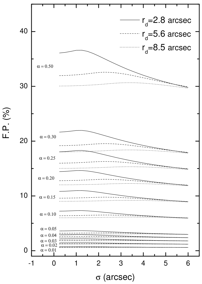
Figure 1: Curves of the simulated fractional polarization as a function of the seeing $\sigma$. Model parameters: $r_{\mathrm{e}}=5$ kpc, $\Delta M_{V}=0$, $z=0.05$. The three aperture sizes are shown for each $\alpha$ (intrinsic polarization).

Figure 2: Curves of the simulated fractional polarization as a function of the seeing $\sigma$. Model parameters: $r_{\mathrm{e}}=5$ kpc, $\Delta M_{V}=-2$, $z=0.05$. The three aperture sizes are shown for each $\alpha$ (intrinsic polarization).

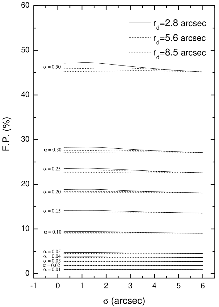
Figure 3: Curves of the simulated fractional polarization as a function of the seeing $\sigma$. Model parameters: $r_{\mathrm{e}}=5$ kpc, $\Delta M_{V}=2$, $z=0.05$. The three aperture sizes are shown for each $\alpha$ (intrinsic polarization).

Considering host galaxies with larger $r_{\mathrm{e}}$ and positive $\Delta M_{V}$ (nucleus brighter than host), the behaviour of the curves is qualitatively similar, but with a much lower decrement of $FP$ with respect to $\alpha$.

3.2 Observational conditions

From Figs. 1 to 3 one can see that all curves show a maximum at $\sigma\approx r_{\mathrm{d}}/2$, although this is more evident for smaller $r_{\mathrm{d}}$ and larger $\alpha$. This behaviour can be explained as follows. At the lowest $\sigma$ values, the aperture contains almost all the flux from the star-like nucleus, plus a part of the non-polarized light from the more extended host galaxy. As $\sigma$ begins to increase, most of the polarized light from the nucleus is spread to an area still within the aperture, whereas a significant part of the unpolarized light from the host galaxy is spread out of the aperture; thus, $FP$ first grows. This happens until the seeing $\sigma$ is high enough that the fraction of (partially polarized) light removed from the nucleus becames larger than the fraction of (unpolarized) light removed from the host, thus lowering FP. The FP maximun is attained when the FWHM ($=\sigma/0.4255$) is approximately similar to the aperture radius: when using larger apertures, a larger $\sigma$ has to be attained before it begins to spread out a significant fraction of polarized light from the nucleus.

The position of the FP maximun for a given aperture size has a very mild, if any, dependence with the host galaxy effective radius (at least, within the range of $r_{\mathrm{e}}$ used for the present simulations). It should depend, instead, on the slope of the convolved host galaxy surface brightness profile at the aperture edge, which determines the relative increment of galaxy light thrown off the aperture as $\sigma$ increases. This slope has only a mild dependence on $r_{\mathrm{e}}$. We verified these points using a set of artificial galaxy images with $r^{\frac{1}{4}}$ profiles convolved with a Gaussian PSF.

One important result from the observational conditions behaviour is that variations in the atmospheric conditions could affect linear optical polarization measurements by introducing a spurious variation component, thus undermining the reliability of microvariability studies on a given source under certain (although rather extreme) conditions. These would require, for example, a highly polarized AGN within a bright host, observed under atmospheric conditions giving place to changes in the seeing from $\sigma\simeq 2$ arcsec to more than $4$ arcsec. These conditions would seem very unlikely to occur, but they are not impossible. In general, telescopes used for the monitoring of AGN variability are not large, modern instruments located at the best astronomical sites, because these kind of studies demand large amounts of telescope time. On the other hand, since astronomical polarimetry is a differential measuring technique, it is usually assumed to be almost immune to mediocre atmospheric conditions. Thus, it might not be so unlikely to face such an extreme situation, with large seeing fluctuations along the observing time.

From our simulations, the changes in the polarization can be divided into three regimes. First, up to $\sigma\simeq 2$ arcsec (FWHM $\simeq 4.5$ arcsec) the change is small. Between $\sigma\simeq 2$ arcsec and $4.5$ arcsec ($4.5\,\textrm{arcsec}<\textrm{FWHM}<10\,\textrm{arcsec}$) the change is higher and faster. From this point up to the highest $\sigma$, the polarization behaviour flattens again. The second regime is, thus, where the most significant spurious variability events should be expected.

The amplitude of any possible spurious variation depends basically on two parameters: the amplitude of the variation of the seeing function, $\Delta\sigma$, and the aperture size. As it can be seen in Figs. 1 to 3, smaller aperture sizes allow a more accurate measurement of the AGN intrinsic polarization (by minimising unpolarized light from the host), but, at the same time, they are the most sensitive to changes in $\sigma$.

On the other hand, when $\sigma$ is high (regardless of whether it remains constant or not), the fraction of polarized light diminishes. This effect is less noticeable for larger aperture radii, because the nucleus polarization is already diluted by a large fraction of host light. Although all models, with all possible combination of the different parameters, do show this behaviour, the incidence of $\sigma$ variations becomes almost insignificant when the nuclei are brighter than their respective host galaxies (Fig. 3). The aperture with radius $r_{\mathrm{d}}=5.6$ arcsec always allows to get reasonably good quality data while, at the same time, it minimises the effects due to changes in the atmospheric conditions.

3.3 Behaviour with redshift

One interesting issue to study is what happens when considering the same system host galaxy+nucleus at different redshifts. The modifications introduced by changing $z$ imply only a geometrical effect, (for the cosmogical model assumed, see Section 2.1). No evolution effects were considered, and note that no additional correction for cosmological dimming was applied, since the fluxes both from the host galaxy and from the nucleus are equally affected by redshift, while K-correction effects can safely be ignored for this study. In Fig. 4, curves for one specific model ($r_{\mathrm{e}}=10$ kpc, $\Delta M_{V}=-2$) are shown. All curves take only the value $\alpha=1$, which corresponds to a fully polarized (i.e. physically unreal) nucleus. However, all the other possible curves will behave in a qualitatively similar way, because $\alpha$ is a multiplicative constant in the equation defining $FP$ (see Eq. 8).

As $z$ increases, the effective radius of the host galaxy in arcsec gets smaller, until most of the flux coming from the galaxy is contained within the aperture. This leads to the following effect: $FP$ gets lower with larger $z$ (at constant $\sigma$) because of a larger unpolarized flux fraction from the host. At the same time, variations of $FP$ with respect to $\sigma$ have lower amplitudes for larger $z$.

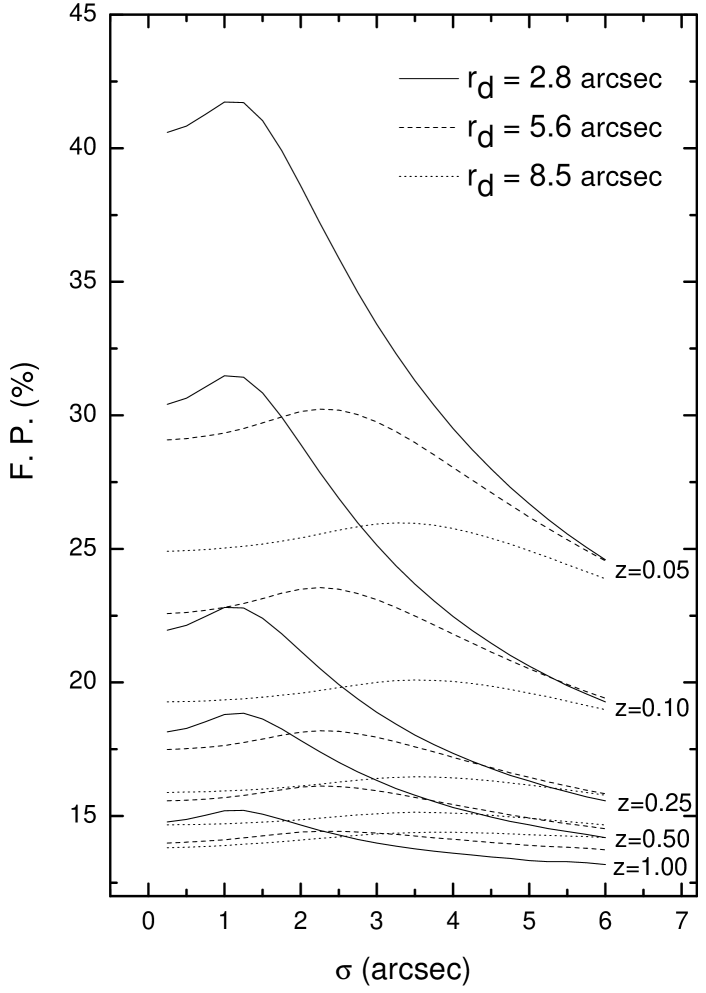
Figure 4: Curves of the simulated fractional polarization as a function of seeing. Model parameters: $r_{\mathrm{e}}=10$ kpc, $\Delta M_{V}=-2$, $\alpha=1$. Three aperture apertures are considered for each value of $z$.

3.4 Temporal behaviour

So far, we have shown that the fractional polarization $FP$ is a strong function of the seeing $\sigma$ under certain particular conditions. We can now ask the question: how much do variations in the atmospheric conditions affect the optical polarization microvariability results for blazars? To study this, we need a seeing temporal behaviour curve. We propose that, by making simultaneous observations of linear polarization and seeing, we can estimate the influence of seeing on the actual polarization of the source.

Figure 5: Temporal evolution of $\sigma$ adopted from measurements made during the monitoring campaign on the optical linear polarization of blazars reported in Andruchow et al. (2005).

In Fig. 5 we present a temporal curve for $\sigma$ built from seeing measurements made at CASLEO during the polarization campaign reported in Andruchow et al. (2005). We can then use this particular seeing curve to calculate the value of $FP$ for each model. In order to do this, and for this particular example, we ran all the simulations again with a $0.01$ arcsec step in $\sigma$ (instead of $\Delta\sigma=0.25$ arcsec as in Sec. 2.2) to have a better sampling. Then we matched each value of $FP$ with its corresponding $\sigma$ for any given time. In this way we obtained the temporal variation curves for $FP$ due only to the changes in the atmospheric conditions. This procedure was carried out for each of the three aperture sizes ($r_{\mathrm{d}}=2.8$, $5.6$, and $8.5$ arcsec).

We found that the variations in atmospheric conditions translate into variations in the calculated $FP$  For the smallest aperture size, the minimum and maximum values of $FP$ are matched with the maximum and minimum on the seeing curve, respectively. This behaviour is hardly distinguishable for the larger aperture sizes. As we already pointed out, with the smallest $r_{\mathrm{d}}$, the maximum amount of polarization is recovered; however, seeing-induced changes can be large. For all models, we found that the best balance between a high detection of polarization and a low influence of seeing-induced variations was obtained with an $r_{\mathrm{d}}=5.6$ arcsec aperture.

Although all models show the same general (qualitative) behaviour, the influence of seeing variations on $FP$ depends on the parameters describing each model. Again, we got that the spurious effects due to seeing variations become negligible when the nucleus is brighter than the host galaxy. And this effect is further enhanced for large $z$, when the host is not only dim but also of small angular size, compared to $r_{\mathrm{d}}$.

4 An Example: Application to PKS 0521$-$365

As an example of the results presented in previous sections, we applied the method to the blazar PKS 0521$-$365. We chose this particular source because it is a well-studied blazar, which has a bright elliptical host galaxy with well-known parameters. Regretably, bad weather conditions prevented us from obtaining additional data of this object under different observational setups (i.e., using different apertures, etc.), and so we had to rely on observations from our monitoring program on the optical linear polarization of blazars (Andruchow et al., 2005). Although this situation does not allow a full testing of our simulations, we judge that the example we present is at least illustrative for our purposes.

The observations were carried out using the 2.15-m Jorge Sahade telescope at CASLEO, San Juan, Argentina, during two consecutive nights on November 2002. The data were collected using the CASPROF photopolarimeter, in an on-off regime, i.e., performing a target observation followed by a near-sky one to allow for the corresponding subtraction of the sky polarization contribution. A few points (affected by poor transparency during the night) were removed after a first analysis. Off-target observations before and after the target pointing were interpolated to increase accuracy in the subtraction procedure. The seeing measurements were made with a DIMM-type monitor placed close to the dome. In Fig. 6 we show the observational results for the two nights along which we followed the source. The error bars are calculated as in Magalhães et al. (1984), from photon-noise statistics. Significant polarimetric microvariability can be seen, at least for the first night.

Figure 6: Temporal behaviour of the degree of polarization, $P$, for PKS 0521$-$365 (upper panels) and the simultaneous seeing measurements, $\sigma$ (lower panels). Left column: observations for the night of Nov. 05, 2002; right column: similar curves for the night of Nov. 06, 2002.

4.1 Specific Model

In order to evaluate which fraction (if any) of the linear polarization variability observed for PKS 0521$-365$ is due to seeing fluctuations, we must now choose the specific model which best represents the object’s structural properties. Using the results of the surveys reported in Scarpa et al. (2000a), Urry et al. (2000) and Falomo et al. (2000), the host galaxy and nucleus parameters that we adopted for PKS 0521$-365$ were:

• $m_{\mathrm{HOST},\,R}=14.60\pm 0.01$ mag,

• $m_{\mathrm{AGN},\,R}=15.28\pm 0.10$ mag,

• $r_{\mathrm{e}}=2.80\pm 0.07$ arcsec,

• $z=0.055$.

The apparent magnitudes are given in the $R$-band of the Johnson-Cousins system. Using the values of the colour index, $V-R$, for the host galaxy and the nuclear point like source from Urry et al. (2000) we obtained the $V$-band apparent magnitudes. With these values, the magnitude difference gave $\Delta m_{V}=\Delta M_{V}=-0.34$. The plots for each aperture size and for all values of $\alpha$ for the corresponding model are shown in Fig. 7.

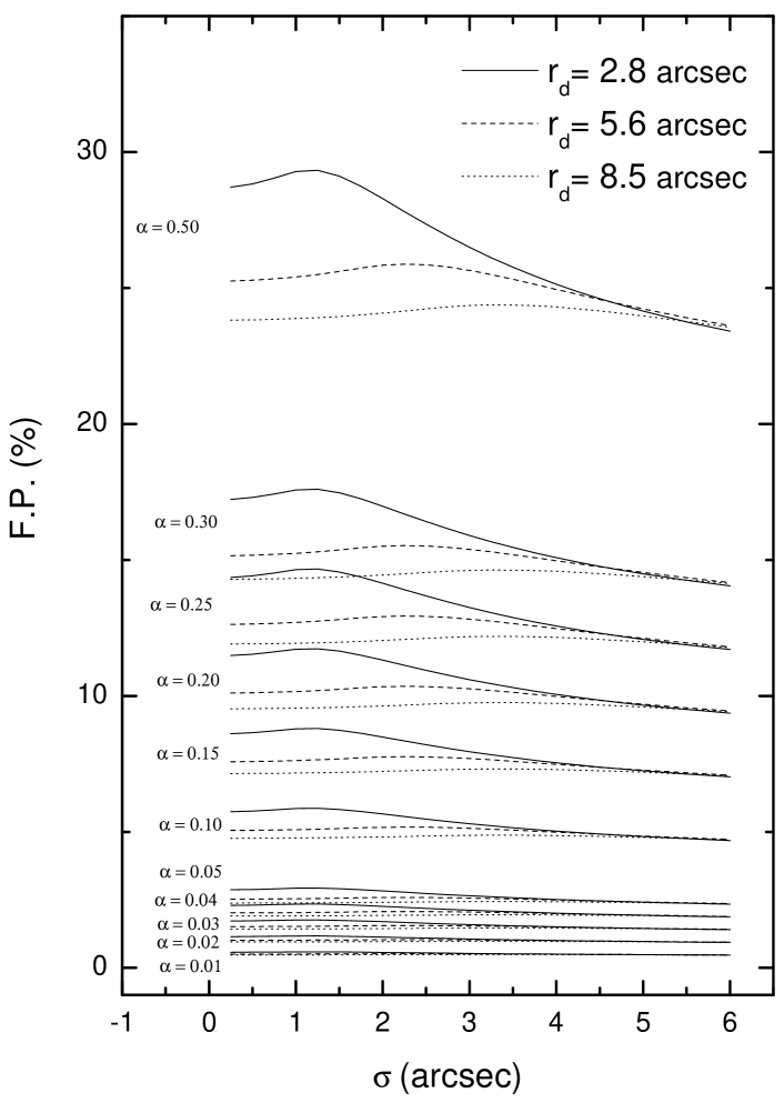
Figure 7: Simulated fractional polarization as a function of the seeing, $\sigma$, for the particular case of the source PKS 0521$-$365. Parameters of the model: $r_{\mathrm{e}}=2.8$ arcsec, $\Delta M_{V}=-0.34$, $z=0.055$. Three aperture values are shown for each $\alpha$.

In Table 1 we present the corresponding observational results for the two nights in which we followed the source in Nov. 2002. Column 1 gives the date; the number of points for each night is given in column 2; column 3 gives the mean polarization values; column 4 shows the respective standard deviations; column 5 is the time difference between the maximum and minimum $P$ values; and column 6 is the variability result, “V” for variable and “NV” for non variable. From the observations, the mean value for the degree of polarization is about $3\,\%$. Using the results from the simulation corresponding to the adopted model, we looked for the value of $\alpha$ which best reproduces $FP=3\,\%$ when $\sigma$ is close to zero for an $r_{\mathrm{d}}=5.6$ arcsec aperture (see also Fig. 7); in this way we adopted $\alpha=0.06$ as the theoretical value according to the models.

This $\alpha=0.06$ (i.e., 6 percent) represents then the intrinsic polarization of the active nucleus. For each night, we took the corresponding seeing measurements and, assuming that the degree of intrinsic polarization was always constant at $6\,\%$, we obtained the behaviour of $FP$ vs. time from the results of the simulations for the chosen aperture.

The variations thus obtained for $FP$ should represent those due only to the fluctuations in the atmospheric conditions during the observing session. In Fig. 8 we show the results: upper panels correspond to the results of the simulations whereas lower panels show the seeing behaviour for each night. The error bars of each point were estimated from the actual observational errors. The average error of each individual observation point was about $5\%$ , so, we adopted this average observational error as the error for each simulated data point. Although the fluctuations have very small amplitudes, the general trend was recovered: this means that the maximum of $FP$ corresponds to the minimum of the seeing and vice versa.

Figure 8: Upper panels: Variation curve of the simulated $FP$ due only to seeing changes as a function of time, for the nights of Nov. 5, 2002 (left) and Nov. 6, 2002 (right). Lower panels: behaviour of $\sigma$ from simultaneous observations. Left column: Nov. 5, 2002. Right column: Nov. 6, 2002.

Table 1: Statistical results of the degree of polarization microvariability for the blazar PKS 0521$-$365. Observations. Here, $n$ stands for the number of observations, $V/NV$ for “Variable” or “Not Variable”, and the remaining symbols have the usual meaning (see text).

Date	$n$	$\langle P\rangle$	$(\mathrm{rms})_{P}$	$\Delta t$	V/NV
$[$d/m/y$]$		[$\%$]		[h]
05/11/2002	6	3.05	0.769	2.1387	V
06/11/2002	8	2.88	0.105	2.1621	NV

Table 2: Statistical results of seeing measurements for each night.

Date	$\langle\sigma\rangle$	$(\mathrm{rms})_{\sigma}$	$\Delta\sigma$	$\Delta t$
$[$d/m/y$]$	[arcsec]			[h]
05/11/2002	0.95	0.10	0.27	2.1387
06/11/2002	1.22	0.15	0.43	1.1627

Table 3: Statistical results of the polarization fraction flux microvariability for the blazar PKS 0521$-$365. Simulations. Meaning of the symbols as in Table 1.

Date	$n$	$\langle FP\rangle$	$(\mathrm{rms})_{FP}$	$\Delta t$	V/NV
${\rm[d/m/y]}$		[$\%$]		[h]
05/11/2002	6	3.05	0.004	2.1387	NV
06/11/2002	8	3.06	0.005	0.6174	NV

4.2 Statistical Results

The way we used to compare observed and simulated values was through the statistical analysis of each data set. In Table 2 we present the results of the statistical analysis of the seeing measurements. Column 1 is the date; column 2 is the mean value of seeing $\sigma$; column 3 is its standard deviation; column 4 is the amplitude of $\sigma$ variations; and column 5 is the time difference between the maximum and minimum $\sigma$. In Table 3 we present the corresponding statistical results for $FP$. The colums have similar meanings to those in Table 1.

The ratio between the dispersion of the observed polarization and the dispersion of the simulated polarization fraction can be used as a quantitative test to assess whether or not spurious (i.e. seeing-induced) variations are significant. In this sense, we propose that, if $(\mathrm{rms})_{P}/(\mathrm{rms})_{FP}>1$ the changes in the night condition do not affect the variability results. Otherwise, if $(\mathrm{rms})_{P}/(\mathrm{rms})_{FP}<1$ the variability result could be modified by a seeing time curve variation. For the case of PKS 0521$-$365, on both nights, this ratio was $(\mathrm{rms})_{P}/(\mathrm{rms})_{FP}\gg 1$; hence, from a statistical point of view, there was no significant spurious variability due to seeing changes in the observed polarization during any of the nights. There is a rather worrisome hint for a broad trend between seeing and polarization time curves during the first night; however, $\Delta P$ is much larger than expected just from seeing variations. We can thus be confident that the variations detected for the source had an intrinsic origin in the blazar.

During the second night, the seeing values were higher and changes occurred with a higher amplitude than during the first night (see Table 2). However, this relatively high amplitude would have not been enough to introduce any spurious variation component by itself. On the other hand, the high seeing values during the whole observational session had direct influence on the data quality. In extreme cases, the larger error bars could have masked possible low amplitude variations.

Probably because of the relatively small amount of polarization shown by PKS 0521$-$365 and to the particular observational conditions during both nights, we were not able to obtain any firm conclusions regarding the influence of changes in the atmospheric conditions on the polarimetric variability results for this particular blazar. In any case, we want to point out that this example shows that the metodology is actually aplicable to a real case. Further studies, involving enough data to improve the statistics, and using different aperture radii, are needed in order to obtain more general results.

4.3 Inference of the intrinsic linear optical polarization

As it is pointed out by Nilsson et al. (2007), it is difficult to have an estimate of the true optical polarization of blazar nuclei. One implication of the approach that we present here is that it allows to estimate a lower limit to the intrinsic value of the active nucleus polarization. As we pointed out in the case of PKS 0521$-$365 observations, by collecting both polarization and seeing data, and knowing the host/AGN photometric parameters and the redshift of the object, we can apply the model results as corrective terms, obtaining an estimation for the true polarization for any given measurement. This estimation is interpretated as a lower limit because, under the assumptions made for our models, at least is needed to have that amount of polarization at the sources in order to reproduce the observational data.

Defining $FF$ as the fraction of the total flux originated in the active nucleus which we measure within a given aperture, the relationship between $FF$ and the value of the observed polarization, $P$ (wich may variate both by seeing and intrinsic causes), is given by:

$$P=\alpha\,FF\,.$$ (9)

The flux fraction $FF$ is thus the right-hand member of Eq. 8 divided by $\alpha$, and is obtained from our models. With this value and the observed polarization ($P$) we can recover the intrinsic AGN polarization ($\alpha$).

Despite of the fact that we find no practical way to provide future observers with a detailed output from our models, serving as “ready-to-use” corrections to their measurements, we can nevertheless give them a few numbers which can serve as a guide to estimate a lower limit of the true (nuclear) polarization. This is done in Table 4, which should be read as a double-entry table with the redshift in column 1, and gives the flux fractions corresponding to the maxima in Figs. 1-4. Column 2 corresponds to an aperture radius $r_{d}=2.8$ arcsec, column 3 to $r_{d}=5.6$ arcsec, and column 4 to $r_{d}=8.5$ arcsec. These maxima correspond approximately to seeing values $\sigma=1.0$ arcsec, $\sigma=2.2$ arcsec, and $\sigma=3.2$ arcsec, respectively for each aperture radius. Note that the positions of these maxima, as said in Sect. 3.2, do not depend on the hosts effective radii (at least for the range in $r_{\mathrm{e}}$ that we used), so we just give our results for the three different magnitude differences ($\Delta M_{V}$) considered in Sect. 2.

We can now go one step further and, by applying the above described process to each individual data point in an observing session (if we are studying a time series), we can follow the behaviour of $\alpha$ during any given observing session. As an example, we applied these ideas to the blazar PKS 0521$-$365 observations. Notice that we are proposing a temporal dependence for $FF$ and $P$. So, Eq. (9) is now re-written as:

$$P(t)=\alpha(t)\,FF(t)\,.$$ (10)

The temporal dependence in $FF$ (and hence in $FP$) is through the seeing $\sigma$ variations. However, the temporal behaviour of the observed polarization $P$ will be due to these seeing-induced variations plus any variability intrinsic to the source. Thus, knowing the temporal behaviour of $FF(t)$ from the models and the seeing measurements, it is in principle possible to recover the actual polarimetric behaviour of the active nucleus, $\alpha$(t), from the observed polarimetric curve $P(t)$.

Applying this to the case of PKS 0521$-$365, we calculated $\alpha$ for each observational instant at the nights of November 5 and 6, 2002. In Fig. 9 we present the temporal variation curves for $\alpha$.

During both nights, since the amplitude of the $FP$ curves was low, the general trend of the curves resulted similar for $P$ and $\alpha$ (see Figs. 6 and 8, upper pannels, for the behaviour of $P$ and $FP$ during the night). These facts can be used as a confirmation of the variability results obtained from the observations. However, in order to have a clearer picture of the different systematics affecting optical polarization measurements in blazars, it would be necessary to test our ideas with other targets. Nonetheless, we mention these first steps because we believe that they may contain a relevant potential for studying what is actually happening at the regions were the optical polarized radiation is generated.

Figure 9: Variability curves for the $\alpha$ parameter in the case of PKS 0521$-$365.

Table 4: Maximum values of $FF$ for the models in Figs. 1-4.

$z$	$FF_{1}$	$FF_{2}$	$FF_{3}$
	$\Delta M_{V}=-2$
0.05	30.20	22.85	20.09
0.10	23.49	18.51	16.88
0.25	18.17	15.81	14.97
0.50	16.10	14.77	14.44
	$\Delta M_{V}=0$
0.05	73.19	65.15	61.33
0.10	65.96	58.91	56.16
0.25	58.36	54.24	52.63
0.50	54.78	52.24	51.56
	$\Delta M_{V}=+2$
0.05	94.51	92.18	90.92
0.10	92.44	90.05	88.99
0.25	89.84	88.21	87.51
0.50	88.43	87.34	87.04

5 Conclusions

We have modelled the incidence of the host galaxy on optical linear polarization measurements for blazars. We show that, knowing the relevant photometric parameters of the host galaxy (effective radius, effective surface brightness, magnitude difference with respect to the active nucleus) and the value of the seeing $\sigma$, an estimate of the intrinsic value of the optical polarization can be obtained. This value is always higher than the observed polarization.

Moreover, if the degree of polarization presented by the blazar is high enough (how high is “high enough” depends on the system nucleus + host galaxy) and seeing time variations do occur (under conditions corresponding to the second regime mentioned in Section 3.2), a spurious component in the measured polarization curve may result, especially for nearby blazars with relatively bright hosts. So, in general, if the seeing remains stable during the night, the most suitable aperture will be a small one, in order to minimize the underestimate of the polarization. On the other hand, if seeing is poor and variable, we found that an intermediate-sized aperture (in our case $r_{\mathrm{d}}=5.6$  arcsec) may give a good compromise between spurious variations obtained with smaller radii and a severe subestimation of the intrinsic polarization obtained with large-sized apertures.

In principle, these spurious fluctuations may be removed from the observed polarization curve, provided that the seeing temporal evolution along the night is known. Simultaneous measurements with a seeing monitor are needed in the case of polarimetric observations done with an instrument like the one used for the present work. CCD polarimetry, on the other hand, has the advantage that the PSF (including instrumental effects besides seeing) can be directly measured on each science frame. However, care must be taken in this case since different PSFs are usually obtained for the ordinary and extraordinary images. Whereas the general conclusions of our work may still apply for CCD polarimetry, a particular modelling will probably be needed in this case.

Acknowledgements: This project was supported by the Argentine Agencies CONICET (GRANT PIP 5375) and ANPCyT (GRANT PICT 03-13291 BID 1728/OC-AR). G. E. Romero thanks support for the National Natural Science Foundation of China (GRANT 10633010). The authors thank CASLEO staff, and they wish to dedicate this paper to the memory of Rebeca Morales; CASLEO will not be the same without her. The authors want to thank the anonymous referee for valuable comments that really helped to improve the present paper.

References

- Andruchow (2006) Andruchow I., 2006, PhD Thesis, FCAGLP-UNLP
- Andruchow et al. (2003) Andruchow I., Cellone S. A., Romero G. E., Dominici T. P., & Abraham Z. 2003, A&A, 409, 857
- Andruchow et al. (2005) Andruchow I., Cellone S. A., & Romero G. E., 2005, A&A, 442, 97
- Antonucci (1993) Antonucci, R., 1993, ARAA, 31, 473
- Capaccioli (1988) Capaccioli, M., 1988, Boletín de la Academia de Ciencias de Córdoba, Vol. 58, Num. 3-4, 317
- Cellone et al. (2000) Cellone S. A., Romero G. E., Combi J. A., 2000, AJ, 119, 1534
- Cellone et al. (2007) Cellone S. A., Romero G. E., Araudo A. T., 2007, MNRAS, 374, 357
- de Vaucouleurs (1948) de Vaucouleurs, G., 1948, Ann. Astrophys., 11, 247
- Falomo et al. (2000) Falomo R., Scarpa R., Treves A., & Urry C. M., 2000, ApJ, 542, 731
- Forte et al. (2002) Forte J. C., Bassino L. P., Vega E. I., Pellizza González L. J., Cellone S. A., & Méndez M. R. 2002, AJ, 123, 3263
- Gadotti (2008) Gadotti, D. A. 2008, MNRAS, 384, 420
- Impey et al. (1982) Impey, C. D., Brand, P. W. J. L., & Tapia, S. 1982, MNRAS, 198, 1
- Kuhlbrodt et al. (2004) Kuhlbrodt, B., Wisotzki, L., & Jahnke, K., 2004, MNRAS, 349, 1027
- Magalhães et al. (1984) Magalhães, A. M., Benedetti, E., & Roland, E. H. 1984, PASP, 96, 383
- Mead et al. (1990) Mead, A. R. G., Ballard, K. R., Brand, P. W. J. L., Hough, J. H., Brindle, C., & Bailey, J. A. 1990, A&AS, 83, 183
- Nilsson et al. (2003) Nilsson, K., Pursimo, T., Takalo, L. O, Sillanp , A. & Heidt, J., 2003, ASPC, 299, 303
- Nilsson et al. (2007) Nilsson, K., Pasanen, M., Takalo, L. O, Lindfors, E. & Heidt, J., 2007, A&A, 475, 199
- Romero et al. (2002) Romero G. E., Cellone S. A., Combi J. A., Andruchow I., 2002, A&A, 390, 431
- Saglia et al. (1993) Saglia R. P., Bertschinger E., Baggley G., et al., 1993, MNRAS, 264, 961
- Scarpa et al. (2000a) Scarpa R., Urry C. M., Falomo R., Pesce J. E. & Treves A., 2000a, ApJ, 532, 740
- Scarpa et al. (2000b) Scarpa R., Urry C. M., Padovani P., Calzetti D. & O’Down M., 2000b, ApJ, 544, 258
- Trujillo et al. (2001) Trujillo, I., Aguerri, J. A. L., Cepa, J. & Gutiérrez, C. M., 2001, MNRAS, 321, 269
- Urry & Padovani (1995) Urry, C. M, & Padovani, P., 1995, PASP, 107, 803
- Urry et al. (2000) Urry C. M, Scarpa R., O’Dowd M., et al., 2000, ApJ, 532, 816