Visualizing Astrophysical N-body Systems
Abstract
I begin with a brief history of N-body simulation and visualization and then go on to describe various methods for creating images and animations of modern simulations in cosmology and galactic dynamics. These techniques are incorporated into a specialized particle visualization software library called MYRIAD that is designed to render images within large parallel N-body simulations as they run. I present several case studies that explore the application of these methods to animations of star clusters, interacting galaxies and cosmological structure formation.
Keywords: stellar dynamics – methods: N-body simulation – methods: numerical – Galaxy: kinematics and dynamics – Galaxy: formation – galaxies: evolution – galaxies: interactions – galaxies: spiral – cosmology: dark matter
1 Introduction
One of the great challenges in numerical astrophysics right now is the simulation of the formation and evolution of galaxies from the initial conditions prescribed by the -CDM cosmological model (?). This model specifies the cosmological parameters and initial power spectrum of density fluctuations and presents an accurate set of initial conditions for the universe emerging from the Big Bang. The difficult task at hand is numerically solving the physical equations governing gravity, gas dynamics, and radiation to understand the details of how the initial state transforms into a universe containing the large-scale structure and galactic population revealed by observations. Modern simulations employ both Lagrangian (particle or N-body) and Eulerian (mesh) methods either separately or as hybrids to follow the evolution of the dark matter and gas and its transformation into galaxies and their stellar populations.
Advances in supercomputing power combined with code development and new efficient algorithms during the past two decades have created marvelous datasets with increasing resolution and realism for comparison to the real universe. Current simulations now contain billions of particles or comparable numbers of mesh elements. These datasets are usually studied like real observations by analyzing the various gross properties and statistics of galaxy-like objects that form in the simulations including masses, scale-lengths, shapes etc. Direct visualization of various physical fields such as the density, pressure and temperature are also a powerful way to convey the dynamical evolution. When image time sequences are joined together to make animations, we develop new intuition into the evolution of structures as well as see the relative importance of competing physical processes in driving structure formation. Visualizations are also important tools for conveying the complexities of nonlinear dynamical equations to an non-expert audience including other scientists and the general public at large.
In this paper, I discuss some techniques for the visualization of gravitational N-body simulations as they arise in both cosmological models and experiments in galactic dynamics. Historically, advances in N-body methods have gone hand in hand with visualization and indeed the motivation for doing the first N-body simulations of galaxies were to reproduce the apparent dynamical features in the beautiful photographic images of spiral galaxies and interacting systems. In §2, I begin by reviewing the historical development of methods of N-body visualization. In §3, I discuss various methods for visualizing different types of particle system with some discussion of the application of basic 3D graphics. In §4, I present some case studies to illustrate the use of these methods taken from the GRAVITAS project, an exploration of the science and art of N-body systems, and then conclude with some remarks on future goals of achieving astronomical photorealism.
2 A Brief History of N-body Simulation and Visualization
A complete history of the development of computing and visualization of gravity cannot be presented here but it is worth looking at some critical events and their importance for advancement and understanding in astrophysics. The fascination with the motion of heavenly bodies stretches back to antiquity and modern physics begins here. There is an interwoven story of both computation and visualization that is told in trying to understand these motions.
Archimedes is said to have constructed a device that could trace the movement of the sun, moon based on the heliocentric models of the day and could be used to make predictions of the timing of eclipses (?). Such a mechanical device was actually retrieved from an ancient Roman wreck near Antikythera dated from the 2nd century BCE and while the purpose of the mechanism is still debated it was likely an analogue computing device that could be used to visualize the motion of the sun, moon and planets and predict their future positions (?). Mechanical armillery spheres and astrolabes were later developed independently by Chinese and Arab astronomers to computing and visualize celestial motions.
The advance of the heliocentric Copernican world view lead to Kepler’s discoveries of the planetary laws of motion. His reduction of Tycho’s detailed observations of Mars path across the sky showed the motion to be the result the combined effect of the Earth and Mars on their own elliptical orbits. The motions of the planets were therefore visualized as confocal ellipses - geometrical curves that could be traced out on paper.
In the Principia Mathematica, Newton clearly defined and solved the two-body problem with the new laws of mechanics and gravity. Clockwork mechanisms called orreries (after the Earl of Orrery who first commissioned one to be built) displayed the motions of the planets in the solar system as predicted by Newton’s classical mechanics. These early visualizations translated Newton’s impenetrable expert work of mathematics of the time into something that a wider audience could easily understand. However, Newton himself realized the computational difficulty in solving the more general N-body problem in the context of the solar system and stated:
The orbit of any planet depends on the combined motion of all the planets, not to mention the action of all these on each other. But to consider simultaneously all these causes of motion and to define these motions by exact laws allowing of convenient calculation exceeds, unless I am mistaken, the force of the entire human intellect. (?) (p. 574)
He could not foresee the development of electronic computing that would eventually permit the approximate (but accurate) solution of the general equations of the N-body problem through numerical methods in the 20th century.111Ironically, modern computers function under the principles of quantum mechanics and so understanding of the full complexity of Newton’s N-body problem required the discovery of new physics to construct the machines which perhaps did require the force of the entire human intellect.
With the development of large reflecting telescopes the universe was opened up to the discovery of the nebulae some of which were the galaxies. Lord Rosse’s sketches of the spiral patterns in the Whirlpool Galaxy (M51), were highly suggestive of a swirling, rotating object. Lord Rosse noted:
The sketches …convey a pretty accurate idea of the peculiarities of structure which have gradually become known to us: in many of the nebulae they are very remarkable, and seem even to indicate the presence of dynamical laws we may perhaps fancy to be almost within our grasp. -The Earl of Rosse (?)
The connection of spiral structure to Newtonian gravity would come later. Chamberlin (?) first conjectured that the spiral nebulae might the remnants of the gravitational tidal interactions of colliding bodies. At that time the concept of a galaxy was not defined so he guessed the colliding objects might be stars. Lindblad recognized the connection of these processes to stellar dynamics and struggled with the problem in the middle of the 20th century. One pioneering advance was carried out by Erik Holmberg (?) in an ingenious table top experiment to study interacting galaxies.
In the era before general purpose electronic computing, Holmberg (?) conceived an experiment which used light-bulbs as proxies for gravitating point masses. Since the intensity of light falls as an inverse square law then the cumulative intensity measured at a given position could be used as a proxy for the net gravitational force from the system. He laid out two disk configurations consisting of 37 particles to represent two interacting spiral galaxies. Forces were “computed” by measuring the intensity from the and directions at the positions of each light bulb and recorded meticulously in a notebook. After a force sweep, the positions of the lightbulbs were changed according to their assigned velocity and measured acceleration over a timestep. After each reconfiguration, the process was repeated and so a numerical integration of the motion of the particles could proceed relatively quickly using light intensity as an analogue computational device. In this way, he provided the first early evidence that tidal encounters of disk galaxies can induce spiral structure using simulation and visualization.
The history of modern computation is interwoven with the solution of the N-body problem and it’s visualization. The first computers like the ENIAC were general purpose and programmable and so applicable to many problems. Computation of trajectories for ballistic firing tables strangely occupied as much as 25% of their time (?)! The application of computing the N-body problem to the fields of stellar dynamics emerged in the early 1960’s with applications to globular star clusters (?) and galaxy clusters (?). Many of the issues related to numerical accuracy and computational efficiency that are still relevant today were discussed by Aarseth & Hoyle (?). Direct N-body methods using typically several hundred particles through the 60’s and 70’s were used to illustrate various problems in the evolution of globular star clusters, collisionless gravitational collapse (?), disk stability (?), cosmological structure formation (?) and interacting galaxies (?). Particle-mesh methods derived from techniques employed in plasma physics (?, ?) permitted much larger numbers of particles and were used at this time to explore the stability of galactic disks (?) and visualizations clearly demonstrated the growth of intrinsic spiral and bar instabilities (See (?) for a discussion of these methods). The seminal work by the Toomre brothers (?) on interacting galaxies demonstrated the power of well-crafted figures to express a physical idea. Using restricted 3-body calculations, they clearly demonstrated the origin of tails and bridges seen in close pairs of galaxies as the result of gravitational tidal interactions rather than some other process. This work was also animated using super 8 film and is perhaps the earliest animated example of a physically based simulation of galaxies (?). Eneev et al(?) also did similar work and created an film animation in the Soviet Union (?).
The growth of computing power through the 80’s combined with algorithmic developments transformed the way the N-body problem was solved and visualization played a continuing major role in the understanding the processes in galactic dynamics and cosmology. The emerging cold dark matter cosmology revealed a rich pattern of clustering that could be compared directly to maps of the large-scale structure (?). In galactic dynamics, the application of particle-mesh methods (?) and the Barnes-Hut (BH) tree algorithm (?) increased particle number from hundreds to tens of thousands permitting accurate representation of self-consistent disk galaxies. Barnes’ stunning simulation of a galaxy group with 64K particles (?) was transformed into one of the first detailed animations of self-consistent galaxy dynamics and had great impact both in scientific understanding as well as public fascination with astronomy. The combination of smoothed-particle hydrodynamics (?) with the tree algorithm by Hernquist (?) further increased the realism associated with the simulation of galaxies.
As the modern methods of computer graphics, rendering and animation explosively emerged in the 90’s they saw applications in astrophysics. The production of the IMAX film Cosmic Voyage in 1996 (?) featured animations of cosmological structure formation from the work of Summers et al(?) and SPH galaxy collisions from the work of Mihos & Hernquist (?) and were created with the help of PIXAR studios and visual artists such as Cox at the NCSA (?). This work raised the bar for the standard of astrophysical animation.
At the present time, the parallelization of N-body algorithms along with specialized hardware has increased the numbers of particles in simulations into the billions. There are now many parallelized N-body codes based on different algorithms including treecodes (?, ?, ?, ?, ?), PM methods (?) along with new PM-tree hybrids (?, ?). These codes running on large parallel supercomputers now permit simulations with as many as 10 billion particles (?). Also notable, is the development of the GRAvity PipE (GRAPE) specialized hardware (?) that permits integration of the direct N-body problem for up to a million particles. Visualization of these enormous datasets has become increasingly challenging from a data management and computational point of view.
Concurrently, many particle visualization packages have been developed with different features depending on the type of simulation and task. Some notable specialized open source interactive packages are Starsplatter (?), Tipsy (?), Partiview (?) and SPLASH (?). Many N-body visualizers also convert their data into 2D and 3D density fields and use a data analysis and visualization package like IDL to make colored maps or volumetric renderings or simply develop their own specialized code using open source graphics libraries such as OpenGL.
In the next section, I will describe some general techniques that are used to render large particle datasets including methods for creating density fields with different viewing geometries along with methods of adding color and optimizing brightness and contrast to enhance detail.
3 Methods
3.1 Rendering particle distributions
The first N-body simulations were represented graphically as dots on X-Y plots. While this was sufficient when particle numbers were less than a few thousand, as particle numbers increased figures of galaxy encounters turned into black featureless blobs. Images of real galaxies are representations of the combined luminosity of hundreds of billions of stars integrated along the line of sight. (We ignore the obscuring effects of interstellar dust for now.) The quantity observed is the surface brightness. A similar interpretation can be applied to dark matter simulations where the simple mass density is represented as an equivalent luminosity density. In some cases it is also useful to represent the particles as individual points of light such as the rendering of a star cluster and we discuss how this can be done realistically as well.
The procedure for estimating the surface density from a particle distribution is straightforward. For orthographic (parallel) X-Y projections, one simply specifies a 2D rectangular domain subdivided in pixels and bins the particle mass in their given pixel according to their position coordinates to create a density field. A particle system is a random subsample of some smooth density field so this procedure is equivalent to integrating the 3D density down a given line of sight to produce the surface density. Surface density maps of this kind can then be converted into a suitable image format e.g., FITS in astronomy and manipulated within an astronomical image viewing software such as SAOImage DS9 or IDL to view grayscale or pseudo-colour renditions.
In low density regions where particle sampling is sparse it is sometimes desirable to use interpolation schemes to smooth the density field either in 2D or 3D. Convolution with a smoothing function with a single scale length (e.g., a Gaussian) can be carried out quickly using the convolution theorem and Fast Fourier transforms. The use of real astronomical point spread functions (PSF) that include diffraction spikes introduces interesting visual effects as we discuss below.
The interpolation scheme of smoothed particle hydrodynamics (SPH) provides a convenient method for estimating the density field from a discrete particle distribution (see Price (?) for a thorough discussion in application to SPH simulations of star formation). The density within any pixel (or voxel) is determined as as sum over particle densities weighted by a kernel function. An advantage of SPH interpolation is that smoothing length is adaptive so particles in lower density regions have larger smoothing lengths. Variable smoothing lengths therefore permit a better estimate of the density in sparsely sampled regions than convolution with a PSF function with a single length scale. SPH smoothed images provide the best images for quantitative analysis.
When particle number densities are relatively high i.e., hundreds of particles per pixel, both of these methods provide similar estimates of the density and appear similar in visualizations. In low particle density regions, the SPH method will be more accurate but individual particles will be smeared out into large-sized blobs many pixels across. Convolution with a single PSF reveals a transition from a smooth density field to a system of discrete particles. In the creation of animations, both methods can be used to represent evolving galaxies and cosmological dark matter structures. The choice of smoothing is usually a matter of taste. SPH interpolated systems can appear overly smoothed and hide dynamical details that may be revealed by moving particles while the discrete look of systems convolved with a single function may appear too noisy to others. For systems such as star clusters, convolution with an astronomical PSF containing diffraction spikes and the inclusion of stellar colors can create images that resemble real astronomical images.
3.2 Basic 3D Computer Graphics
The calculation of orthographic surface density images assumes that rays are parallel to the line of sight. Sometimes it is interesting to place the camera nearby or immersed within a particle system thus introducing visual perspective. Systems containing structure on many scales such as seen in simulations of cosmological structure formation can then be appreciated more fully. A camera can also be dynamic moving along a trajectory with a changing viewing direction to create animations. Animations of rotations and fly-throughs give a sense of the relative size and shape of structures in 3 dimensions.
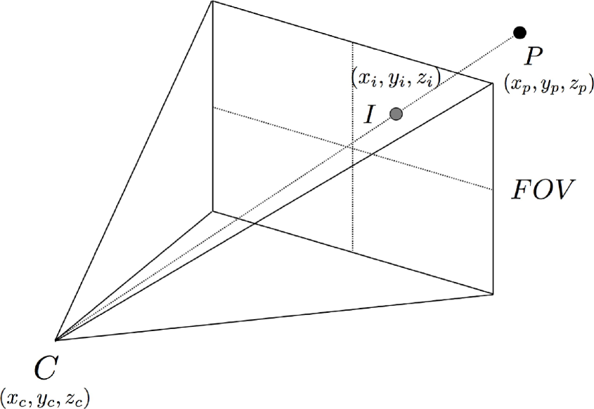
The geometry of perspective for a single particle is given in Figure 1. The pyramidal volume containing the system is called the frustrum. A camera at position is centered on the field of view (FOV) represented by a rectangle placed at a distance . A ray traced from particle hits the FOV to create an image position with coordinates given by:
| (1) | |||||
| (2) |
One can create surface density maps by binning mass on the FOV in the same way as parallel projections. The curvature of the FOV is ignored in this way and noticeable distortion similar to wide angle photographs can be detected near the edges when the angular width of the FOV is greater than approximately .
In practice, a camera is specified by a position in space and an orientation specified by a normal vector perpendicular to the image plane pointed in the viewing direction. For a distribution of particles, one first rotates the particles into the camera’s frame of reference with the viewing direction aligned with the -axis and then take a “picture” by computing the surface density map long this line of sight. A simple way of obtaining the rotation matrix is through the use of quaternions (?). Quaternions are 4-valued quantities composed of a vector and scalar that compactly encode rotation through an angle about a given axis defined by the normal vector . The quaternion coordinates are:
| (3) | |||||
| (4) | |||||
| (5) | |||||
| (6) |
The corresponding rotation matrix used to rotate particles about the defined axis is given by:
| (7) |
One way to determine the rotation matrix for a camera pointing in the direction of the normal vector is to find the axis in the plane that rotates through the angle . This axis lies along the line joining the origin to and it is straightforward to construct the quaternion and resulting rotation matrix.
It is possible to move a camera through space with a variable position and orientation to generate an animation through an image sequence of either a single N-body snapshot or series of evolving snapshots. Rotations and fly-throughs are common applications of moving cameras and we examine some examples below.
3.3 Full Sky and Dome Projections
Full sky and dome projections are sometimes used to depict astronomical datasets. For example, an artistic panorama of the Milky Way in galactic coordinates in an Aitoff projection based on real coordinates was created by Lundmark Observatory in the 1950’s (?). More recently, Axel Mellinger (?) has created a similar panorama digitally from wide field astrophotograpy. Full sky maps of the cosmic microwave background radiation have also been produced to present the primordial density fluctuations recovered from the COBE and WMAP experiments (?). Astronomy borrows transformations from cartography for mapping the objects on the surface of a sphere to a flat display. Two commonly used forms in astronomy are the Hammer-Aitoff (H-A) projection for full sky presentations and the Azimuthal-Equidistant (AE) projections for hemispheres.222see http://en.wikipedia.org/wiki/Map_projection#Equal-area The AE projection is used to create dome masters - flat circular images - for digital planetarium content and resembles the images produced by a fish-eyed lens in photography.
For the H-A projection, the general latitude and longitude coordinates are transformed into an pair that fills a 2:1 flat elliptical domain. In astronomy, are usually identified with galactic coordinates . This projections preserves area on transformation so the relative angular size of objects is unchanged although there is some distortion near the edges of the domain. The transformation is:
| (8) | |||||
| (9) |
Particle positions are transformed this way to a planar domain allowing the creation of surface density maps.
To generate dome master images, it is easier to transform to spherical coordinates first. If particles are centered on the view point and have spherical coordinates then the azimuthal equidistant projection can be defined simply as:
| (10) | |||||
| (11) |
We can compute the spherical coordinates in the standard way from , and . Normally, the radius is cut off at so only one hemisphere is shown. Digital planetariums transform images from this projection typically resolved with pixels. Image processing software divides the dome masters into multiple images that are simultaneously projected onto a dome to create a seamless image (?).
We will discuss the application of both of these projection methods in the case study of animating the collision of the Milky-Way and Andromeda galaxies.
3.4 Color and Brightness
The surface density maps created in any projection are single valued and so by default produce black and white images. There is usually a large dynamic range in the values of projected densities so the default linear mapping of density to a pixel with an 8-bit gray intensity value masks all detail. This problem is overcome by “stretching” the linear intensity through either a power-law (gamma) or logarithmic transformation though a variety of transformations are available depending on the dynamic range of the data. Similar transformations are applied to CCD images from modern telescopes to create published images of galaxies and nebulae.
A variety of colour maps are available in standard image processing software like IDL and SAOImage that map particular stretched gray scale values to different colors. While color maps are excellent ways of conveying physical detail and quantitative information they sometimes are lacking in aesthetic appeal. I present some alternative ways of colorizing N-body simulations by assigning individual colors to particle subsets.
In the case of simulated galaxies, a large fraction of the particles are intended to represent stars or stellar populations so it makes sense to color them with the pallette of natural stellar hues. The color we perceive in an astronomical image comes from the synthesis of a large number of sources with different intrinsic colors and luminosities. How do we calculate the final luminosity and color of a image composed of a combination of different sources? Our eyes perceive the spectral energy distributions (SEDs) of luminous source in terms of color and brightness quantities that can be be reduced to three numbers. Modern computer monitors and digital images encode color with 24 bits (or more) represented by the 3 8-bit values of red, green blue or RGB. RGB color is convenient to work but the net RGB values from a combination of different sources cannot be determined additively. A convenient color triplet for color synthesis is the set of CIE XYZ tristimulus values (?). These values quantify the human response to color through 3 weighting functions , , and that were determined from the statistics of experiments involving human subjects. The CIE XYZ values are calculated by integrating the product of the SED with the weighting function over all wavelengths:
| (12) | |||||
| (13) | |||||
| (14) |
(Note that the response drops to zero outside the visible range accessible to the human eye). The value Y is known as the luminance or net brightness in the absence of color. The normalized pair of values (x,y) are known as the chromaticity coordinates and are given by:
| (15) | |||||
| (16) |
with inverse transformations
| (17) | |||||
| (18) |
The chromaticity coordinates define a “pure” color in the absence of brightness. An object’s color can therefore be disentangled from it’s brightness. Since images and displays used RGB color, we need to convert XYZ triplets back into RGB. There are various RGB systems some of which are device dependent. For example, one device independent definition system is Rec. 709 RGB and conversion from XYZ to RGB can be done with the matrix transformation under the assumption that .
| (19) |
Normally, RGB colors are constrained to lie between 0 and 1 so all RGB values outside of this range are clipped to 0 or 1 depending on where they exceed the range. For our purposes, we do not necessarily need to achieve a perfect true color representation of simulated galaxies so the above transformation matrix is satisfactory though other ones can also be used.
Since the XYZ color values are proportional to the emitted energy, then the net value of the XYZ color from combinations of luminous sources with different SEDs is simply a sum of the independent XYZ values. Therefore when binning a system of particles (stars) with different brightnesses and colors into pixels to create surface brightness (density) maps, one can compute the net value of XYZ for the pixel simply by summing over particles. The chromaticity coordinates can be determined to find the pure color of that pixel along with the luminance Y. Since the brightness profiles are usually sharply peaked in astrophysical objects then luminance can be replaced by a transformed value to bring out detail in the faint regions.
A simple logarithmic transformation
| (20) |
enhances detail well where is a free parameter with being a good choice and is a reference intensity near the maximum value in the image.
Another tranformation is a power-law or gamma transformation is:
| (21) |
where is a power-law typically less than 1 and again is a threshold luminance usually near the maximum value in a map. Pixels can then be colored according to the chromaticity coordinate determined during the creation of the map. Finally, after these transformation images can be improved further by adjusting the values of the brightness and contrast using a variety of tools. The degree of adjustment will depend on the dynamic range of the luminance in the image.
To summarize, we can colorize N-body surface density maps using a simple color map that maps a gray value to a specific color or through color synthesis using CIE XYZ tristimulus values. With color synthesis, we assign individual stars their own unique colors and luminance expressed as an XYZ triplet. we then generate three independent surface density maps for each tristimulus value X, Y, and Z or alternatively we generate surface density maps for different subsets of particles assigned different colors. Since the XYZ color values are proportional to emitted energy then we can sum over particles when binning in pixels to create an image. We determine the pure color of each pixel from the chromaticity coordinates (x,y) derived from each triplet. We can also stretch the luminance Y in each pixel stretched with an appropriate transformation to reveal faint detail and then color with the derived chromaticity. The RGB colors of each pixel calculated with the linear transformation above create the final color image. We discuss applications of color synthesis below in case studies of star clusters and galaxy collision simulations.
3.5 MYRIAD: An N-body visualization software library
Many of the ideas discussed above are the basic elements of standard 3D rendering packages mentioned in §2. Rendering astrophysical particles in the absence of an absorbing medium is basically straightforward since the particles are simply luminous, transparent points obviating the need for complex raytracing. The main difficulty at the current time is dealing with datasets that now contain billions of particles. While rendering single images is not difficult, creating animations of evolving datasets with fine time resolution can be cumbersome. Large file sizes make saving numerous N-body snapshots prohibitive since storage space can be limited and I/O operations can be slow.
One solution to this problem is to integrate a visualization software library with the N-body code itself. The task of rendering many types of images is small in comparison to computing the gravitational (and hydrodynamic) forces in simulations so images from multiple cameras at different positions and orientations can be taken at small time intervals. Large N-body simulations today are done on parallel supercomputers and most algorithms distribute particles among the computing nodes almost equally. Raw surface density maps from a static or moving camera position can be created in parallel on different processors. The final image can be synthesized by summing over partial images generated independently on computing nodes.
I have developed a software package called MYRIAD that creates raw binned surface density maps from particle distributions as orthographic projections, perspective images from static or moving cameras, full sky or full dome projections and stereoscopic images. Post-processing software is used to apply color synthesis methods by blending raw images for different ranges of particles assumed to have different colors or different color bands as well as applying convolutions with different point spread functions to either simply smooth images or add star-like characteristics for bright pixels. The rendering software has been integrated with the parallel N-body codes PARTREE (?) and GOTPM (?) so that image sequences are created during simulation runs. The package can also be used to generate single images or sequences on a single data snapshot through a command line programme. In this way, it has been possible to create sequences with thousands of images in large simulations without the need to save the same number of N-body snapshots.
I will now discuss specific applications of visualization in both galactic dynamics and cosmology that have used MYRIAD to create images and animations.
4 Case Studies
The dynamics of gravitating systems of particles representing galaxies and the cosmological large-scale structure are not only scientifically interesting to astronomers but also a source of beauty and wonder to a more general audience. Over the past few years, I have been involved in a project called GRAVITAS that attempts to express both the scientific complexity and artistic beauty of Newtonian gravity and dynamics revealed through N-body simulation. Animations of star clusters, spiral galaxies, galaxy interactions, galaxy clusters and the large-scale structure are rendered in a variety of ways with fine time-resolution. The animations are accompanied by original music by modern classical composer John Kameel Farah who crafted pieces to reflect both the evolving imagery and scientific ideas in the animations. All of the animations are available in a variety of formats including DVD and free downloads at resolutions up to high-definition can be obtained at our website (?).
4.1 Cosmological Simulations
Cosmological simulations reveal the evolving gravitational framework of the universe as seen in dark matter. They begin when the universe is nearly homogeneous and featureless and show the growth of complex structure through the hierachical collapse of primordial density fluctuations. Small objects condense first and merge to form larger objects that become the dark matter halos of galaxies and galaxy clusters.
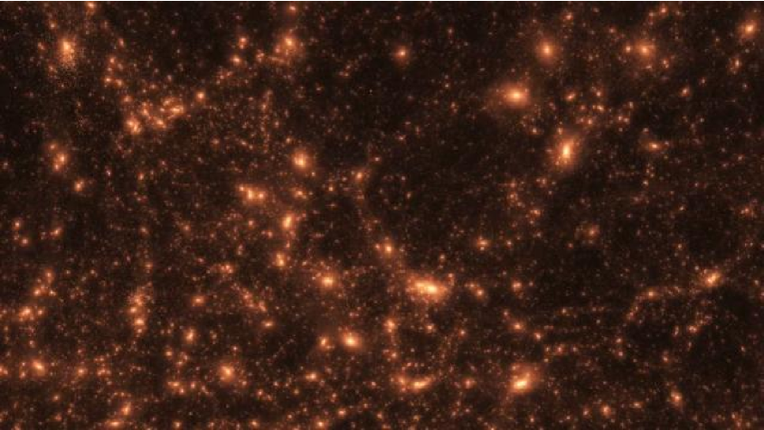
The first application involved the rendering of a flight through a cosmological dark matter simulation (Fig. 2). I used the code GOTPM code to simulate the formation of structure within a periodic cube 100 Mpc on a side with initial conditions determined by the currently favoured parameters of the -CDM model using particles. The simulation was computed on a parallel cluster using 256 processors at McMaster University funded by the SHARCNET collaboration. In cosmological simulations, the particles are confined to a periodic cube and the equations of motion are integrated in co-moving coordinates to null out the cosmic expansion. To emphasize the growth of structure, N-body images are rendered in co-moving coordinates at each of the 5000 timesteps.
The image parameters, camera coordinates and viewing direction are specified through a data file provided to the MYRIAD software. The camera was set on a straight line course at constant speed in co-moving coordinates so that it would fly through the cube twice over the course of the run. We replicated one layer of the cube so that the camera would never get closer than one cube edge length from the edge of the particle distribution. In the end, the renderer looped through 27 billion particles at each step to check which particles were in the field of view for creation of the surface density maps. The camera’s field of view was set to one radian along the widest dimension in frames that were rendered at Cinematic 4K resolution (4096x2160 pixels). A surface density map was created from the moving camera at each integration timestep for a total of 5000 images. The gray images were smoothed slightly with a Gaussian PSF and then enhanced and colorized with a hue that changed gradually from blue to deep red over the course of the simulation as an artistic way to convey the aging of the universe.
A single snapshot from the last frame representing the system at the current redshift is shown in Fig. 2 and reveals the dark halos from the scale of galaxies to galaxy clusters. The accompanying animation shows the evolution of dark halos from a homogeneous beginning through the hierachical collapse and merger of smaller structures emerging from the primordial density fluctuations. At this resolution, we can see substructure within the largest dark halos in the form of orbiting dark matter satellites.
4.2 Nightfall
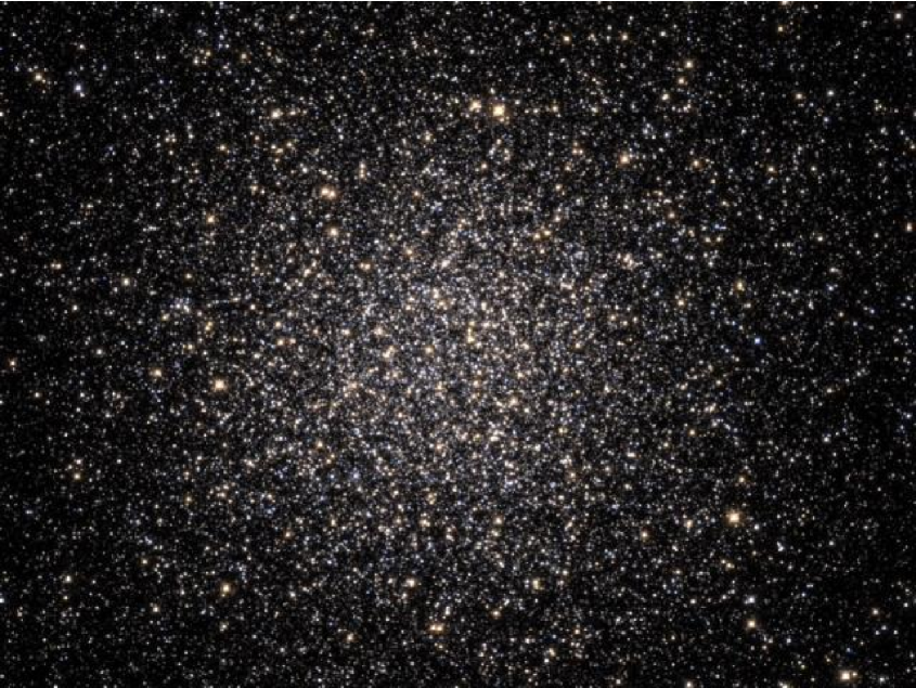
Globular star clusters are one of the purest expressions of Newtonian gravitational dynamics in the universe. They are also the oldest objects in the galaxy and have a distinctive distribution of stars reflecting an old population that is visually dominated by a red giants and blue horizontal branch stars as can been seen in images of globulars from the Hubble space telescope. These objects have been fascinating to astronomers and amateurs alike. Asimov (?) in his classic pulp science fiction story “Nightfall” tells the tale of a civilization on a planet in a multiple star system in a globular cluster. The people of this world are driven to insanity when all of their suns set for the first time in thousands of years revealing a night sky filled with tens of thousands of bright stars. Robert Burnham, Jr. (?) speculates on how the sky might appear inside the Hercules globular cluster M13:
”The appearance of the heavens from a point within the Hercules Cluster would be a spectacle of incomparable splendor; the heavens would be filled with uncountable numbers of blazing stars which would dwarf our own Sirius and Canopus to insignificance. Many thousands of stars ranging in brilliance between Venus and the full moon would be continually visible, so that there would be no real night at all on a planet in a globular cluster.
Inspired by real pictures and these speculations, I created a realistic and dynamic view of a globular cluster over a few hundred orbital times using the treecode PARTREE. For the particle distribution, I use a 1 million particle King model (?) - one of the standard, isotropic distribution functions that are used to model globular clusters. I assume that each particle is just a star of a given visual magnitude and photometric color using a table of data for M15. The color index can be mapped to an effective temperature to estimate a stellar color. The tristimulus color indices of the black-body radiator at the effective temperature for each star were computed by integrating over the blackbody intensity function and then normalized to stellar luminosity measured by the absolute magnitude . This is an approximation but gives colors that are close to the true values.
At each step of the simulation a surface density map for each of the three tristimulus values was created for the particle distribution. In these maps, individual lit pixels tended to represent single stars. Each map is also convolved with a PSF generated by the Tinytim package (?) used to characterize the properties of the PSF in the Hubble Space Telescope (HST) wide field cameras. A typical HST camera PSF has diffraction spikes that become apparent for bright stars and so added another dimension of realism to the images (Fig. 3). The apparent brightness of stars was also allowed to vary depending on the distance from the camera following a intensity law so that approaching or receding stars would brighten or dim. This effect added a further sense of depth to the animation. Finally, for a camera path we choose an inspiralling trajectory that keeps the camera directed to the center of the cluster starting from a distance that reveals the crowded cluster core. In this way, we get a 3D sense of the structure of the cluster and also witness the dynamics of the stars as we approach the center of the stellar distribution.
4.3 Milky Way - Andromeda Collision
Galaxy collisions are dramatic and visually stunning examples of gravitational dynamics on the large scale. The mutual tidal forces of closely interacting disk systems excite 2-armed spiral structure that throw off long tails of stars and gas. The loss of orbital energy to random internal motions lead to the merger of the disks and transformation into an elliptical galaxy. The unravelling of the disk systems leads also patterns of shells and ripples that are themselves another reflection of the physical beauty of phase-mixing in collisionless particle systems. The desire to simulate the complex dynamics of galaxy interactions has been one the main motivations for developing new N-body methods and visualization methods and the animations I describe below continue in this tradition.
One of the more exciting popular astronomical “facts” to emerge in the last decade is that our own galaxy, the Milky-Way (MW) seems to be on a collision course with our neighbour spiral galaxy Andromeda (M31) (?). This idea originates from the original interpretation of the MW-M31 system as a bound pair of orbiting galaxies by Kahn & Woltjer (?) in the so-called timing argument. More recently, modelling of motions in the Local Group of galaxies suggest that this collision may occur within the next few billion years (?). This is a compelling timescale since most eschatological discussions of the Earth’s fate are focussed on the influence of the evolving and warming Sun and it’s eventual transformation into a red giant - a process that occurs on a somewhat longer timescale of 5 billion years. Before that final end, the MW may very well collide and merge with M31 creating a new list of disaster scenarios to explore for the Earth’s possible demise. A simulation of the MW-M31 collision is certainly worth a look both as a specific example of a galaxy collision in action as well as compelling story that may involve the fate of the Earth and solar system and any life that might still be hanging around in a few billion years. Cox & Loeb (?) have even written a scientific paper recently that claims predictions for the eventual fate of the Sun based on model-dependent assumptions. I discuss here my own simulation which is more speculative but does incorporate known constraints on the positions, motions and mass distributions of the two galaxies. The idea is not to quantify the statistics of our eventual fate but rather to explore one detailed scenario to give a sense of what may happen and what it might look like to an Earth observer.
The initial conditions for the collision are described in Dubinski et al(?) in a discussion of the formation of tidal tails in galaxy interactions. The galaxy orientations, relative distance and positions are defined here for specific galactic models that have dimensions, rotation curves, and mass distributions similar to the Milky-Way and M31. These original simulations only used around 30K particles but the models have been re-run with more particles over the years in various demonstration calculations (?, ?) with the recent largest version containing more than 300M particles on a parallel supercomputer in Toronto in 2003 (?).
4.3.1 Spiral Metamorphosis
In this animation, the collision is depicted from a static camera placed at a distance of 320 kpc from orthogonal directions aligned with the galactic plane. Two versions of the animation were created. The first animation uses 300M particles (Fig. 4) and presents two orthogonal projections with a face-on and edge-on view of the Milky Way. A second smaller 30M particle simulation was used to generate a stereoscopic rendering that was converted to a red-cyan anaglyph for viewing with colored stereo glasses. For stereoscopic rendering, one simply takes pictures of the same view from two cameras separated by a small angle (see Bourke (?) or McAllister (?) for an explanation of techniques of stereoscopy). A unique feature of these animations is the fine time resolution compared with other renditions in recent years. Each viewpoint is rendered with 5300 steps covering 2.3 billion years or 440K years per step starting a few hundred million years before the first close passage of the two galaxies. At 30 frames per second, time passes at the rate of 13 million years per second. At this rate, the animation of the collision takes nearly 4 minutes revealing great detail while enhancing the majesty of the event.
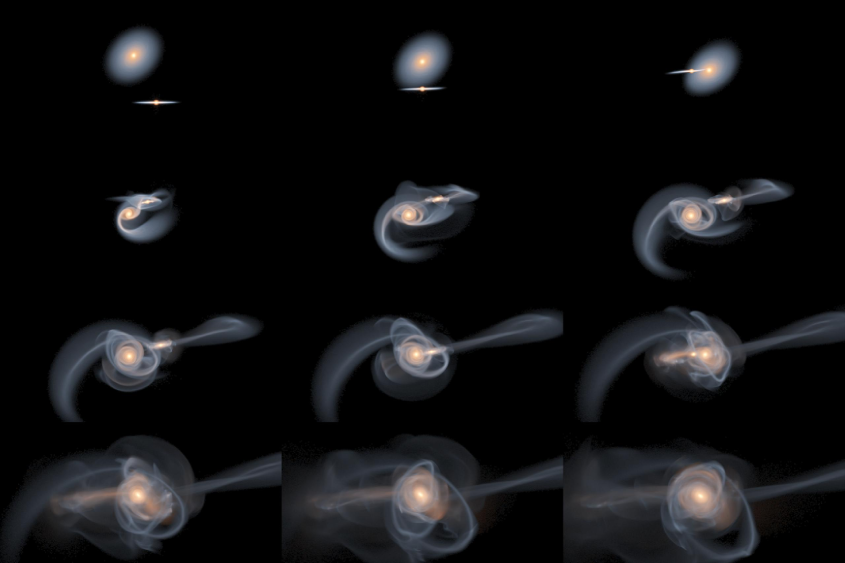
Only the particles representing stars were rendered in these animations with the dark matter left invisible. I used a simple two color scheme to represent old (red) and blue (young) stellar populations and the raw images were convolved with a Gaussian PSF. The chosen tristimulus colors were generated from the SED of young and old populations generate using Bruzual & Charlot (?) models obtained from Bob Abraham (?). The derived colors are close to those depicted in “true” color Hubble images of interacting galaxies like NGC 4676 “The Mice”. Bulge stars were colored red while the disk stars were colored both red and blue with the probability of being red increasing towards the center of the Galaxy. I assigned an exponential probability as a function of gravitational binding energy within the galaxy potential with a functional scale length that would show a gradual color transition from red to blue from the inner to outer disk. In this way, the initial galaxy models have appearances similar to true color images of spirals like M31. As the galaxies interact and eventually merge, the blending of the two stellar colors create an interesting result.
At this high resolution, one should note that the initial model galaxies are extremely smooth and gravitational instabilities that generate spiral structure from the Poisson noise are greatly suppressed. These animations present an idealized depiction of a smooth stellar distribution and are missing the knotty structure of real spiral galaxies containing clumps of gas and new star formation regions. The obscuring dust is also missing so the familiar dust lanes seen in real galaxies is not apparent. The current space show at the Hayden Planetarium in New York presents a depiction of the MW-M31 collision that includes gas and star formation along with dust obscuration using a few million particles.
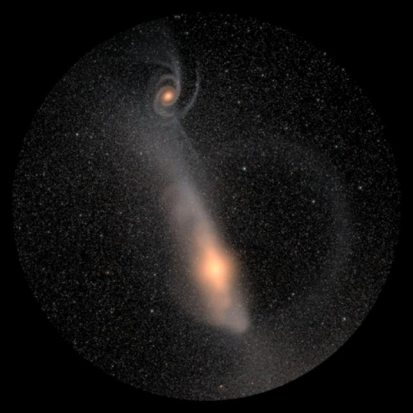
4.3.2 Future Sky
This animation uses the full sky Hammer-Aitoff projection and the Azimuthal-Equidistant projection for planetatrium dome masters to present the MW-M31 collision from the perspective of the Sun. This animation was presented at the Computer Animation Festival at SIGGRAPH 2006 (?) and the dome version was also used for a special presentation at the Gates Planetarium in 2006 (see Figures 5 and 6). One particle on a circular orbit at the solar distance of 8 kpc from the center of the MW model is labelled as the Sun and acts as the platform for the moving camera. As the system evolves, the position of this particle is provided to the image rendering software as the origin for the full sky projections. Initially, the line from the Sun to center of the bulge represents the X-axis in galactic coordinates. We assume future observers will continue to use this convention and define a galactic coordinate system based on this axis and the normal vector to the initial Galactic plane. To track the bulge, we add another particle to the simulation with the mass of a supermassive blackhole in the center of the bulge of the MW. This particle is also given a large gravitational softening length to prevent undesirable dynamical evolution of the bulge. Because of the effect of dynamical friction this particle remains within the dense center of the bulge and therefore acts as a bulge center reference point. We re-orient the particles at each step into a new galactic coordinate system that is defined by the X-axis of the line joining the sun to the blackhole at the bulge centre and the original normal vector to the MW galactic plane. In this way, the bulge tracked by the blackhole always lies along the central meridian in the H-A projection and initially the band of light representing the midplane of the Milky-way remains aligned with the equator. At later times, when the Sun is thrown out of the plane, the bulge begins to show apparent oscillatory motion along the meridian. The bulge also grows and diminishes in size as the Sun rides on a plunging radial orbit that takes it through the center of the bulge.
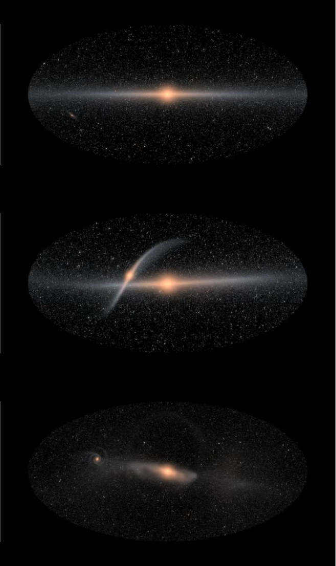
As a small trick, we use the PSF from the Hubble Space Telescope even though the the images show the full sky. In this way, very bright nearby stars have both a noticeably larger diameter and spikes enhancing the impression of brightness and proximity while dim stars are more point like. One final adjustment is the transformation of the linear intensity using logarithmic transformation. In this way, faint interesting details are enhanced and can be seen beside the brightest nearby stars.
5 Conclusions
The visualization of N-body systems has evolved from simple dotted figures a few decades ago to detailed computer animations with billions of particles incorporating the latest developments in 3D computer graphics methods. Numerical astrophysics is an experimental science and the images and animations that are created from simulations are valuable tools for interpreting the results and comparing to observations of the real universe. A well-crafted visualization is a powerful way of conveying detailed physical processes to a general audience and greatly enriches understanding of phenomena.
I have presented some specialized methods for rendering images and animations of large N-body simulations that build on basic principles of 3D computer graphics. The techniques described are straightforward and relatively easy to implement and many groups have replicated the effort in different software. The main new development here is is the ability to render animations with fine time resolution efficiently in parallel supercomputer simulations by integrating the visualization library MYRIAD with an N-body code. I have provided case studies of creation of a selection of animations from the GRAVITAS project that explore different features of the library.
As the resolution of simulations increase, model galaxies are beginning to look more and more like the real thing. The iconic Hubble color images of galaxies are good working definitions of an expression of the visual reality of the universe. A challenging goal for the near term might then be to create photo-realistic animations of the dynamics of galaxies that resemble the Hubble images using our best N-body models of galaxies containing gas, stars and dark matter. The methods I describe here only describe renderings of purely stellar galaxies while the dust lanes and star forming regions of real spiral galaxies are ignored. Simulations of galaxies including gas dynamics, star formation and AGN feedback are being carried out by different groups now (eg., Di Matteo et al(?), Governato et al(?)) and resolution is increasing as well though the extra computational cost of including gas have kept simulation particle numbers to a few million. The animation of the MW-M31 galaxy collision the planetarium show “Cosmic Collisions” created by the Hayden Planetarium is a beginning in that direction of simultaneously rendering stars and the obscuring affect of interstellar dust in an animation. Another factor of 10 to 100 in particle numbers is probably required to approach a truly realistic view.
Acknowledgments
I acknowledge the Canadian Institute for Theoretical Astrophysics (CITA) and the Shared Hierarchical Academic Research Network (SHARCNET) for providing supercomputer time for simulations and visualizations. Research funding was provided by NSERC. I also acknowledge helpful discussions with Bob Abraham, Ka Chun Yu, Frank Summers, Alar Toomre, and Rachid Sunyaev.
References
References
- [1]
- [2] [] Aarseth S J 1963 M.N.R.A.S. 126, 223–+.
- [3]
- [4] [] Aarseth S J & Hoyle F 1964 Astrophysica Norvegica 9, 313–+.
- [5]
- [6] [] Aarseth S J, Turner E L & Gott, III J R 1979 Astrophys. J. 228, 664–683.
- [7]
- [8] [] Abraham R 2002 private communication.
- [9]
- [10] [] Asimov I 1941 ‘Nightfall’ Astounding Stories.
- [11]
- [12] [] Barnes J E 1989 Nature 338, 123–126.
- [13]
- [14] [] Barnes J & Hut P 1986 Nature 324, 446–449.
- [15]
-
[16]
[]
Bourke P 2007 ‘Stereoscopy, theory and practice’ website.
*#1 - [17]
- [18] [] Bruzual A. G & Charlot S 1993 Astrophys. J. 405, 538–553.
- [19]
- [20] [] Burnham R 1978 Burnham’s celestial handbook. an observers guide to the universe beyond the solar system New York: Dover, 1978, Rev.ed.
- [21]
- [22] [] Chamberlin T C 1901 Astrophys. J. 14, 17–+.
- [23]
- [24] [] Cox D J 1996 SIGGRAPH 96 ACM SIGGRAPH p. 129.
- [25]
- [26] [] Cox T J & Loeb A 2008 M.N.R.A.S. pp. 333–+.
- [27]
- [28] [] Davis M, Efstathiou G, Frenk C S & White S D M 1985 Astrophys. J. 292, 371–394.
- [29]
- [30] [] Di Matteo T, Springel V & Hernquist L 2005 Nature 433, 604–607.
- [31]
- [32] [] Dubinski J 1996 New Astronomy 1, 133–147.
- [33]
- [34] [] Dubinski J 2006a in ‘SIGGRAPH ’06: ACM SIGGRAPH 2006 Computer animation festival’ ACM New York, NY, USA p. 209.
- [35]
- [36] [] Dubinski J 2006b Sky and Telescope 112(4), 30–36.
- [37]
-
[38]
[]
Dubinski J & Farah S 2008 ‘Gravitas: Portraits of a universe in
motion’ website.
*#1 - [39]
- [40] [] Dubinski J, Humble R J, Loken C, Pen U L & Martin P G 2003 17th Annual International Symposium on High Performance Computing Systems and Applications.
- [41]
- [42] [] Dubinski J, Kim J, Park C & Humble R 2004 New Astronomy 9, 111–126.
- [43]
- [44] [] Dubinski J, Mihos J C & Hernquist L 1996 Astrophys. J. 462, 576–+.
- [45]
- [46] [] Eneev T M, Kozlov N N & Sunyaev R A 1973 Astron. Astrophys. 22, 41–+.
- [47]
-
[48]
[]
Freeth T, Bitsakis Y, Moussas X, Seiradakis J H, Tselikas A, Mangou H,
Zafeiropoulou M, Hadland R, Bate D, Ramsey A, Allen M, Crawley A, Hockley P,
Malzbender T, Gelb D, Ambrisco W & Edmunds M G 2006 Nature
444(7119), 587–591.
*#1 - [49]
- [50] [] Governato F, Mayer L & Brook C 2008 ArXiv e-prints 801.
- [51]
- [52] [] Heath, T. L., ed. 2002 The Works of Archimedes New York: Dover, 2002, Rev.ed.
- [53]
- [54] [] Hernquist L & Katz N 1989 Astrophys. J. Supp. 70, 419–446.
- [55]
- [56] [] Hohl F 1971 Astrophys. J. 168, 343–+.
- [57]
- [58] [] Holmberg E 1941 Astrophys. J. 94, 385–+.
- [59]
- [60] [] Kahn F D & Woltjer L 1959 Astrophys. J. 130, 705–+.
- [61]
- [62] [] King I R 1966 Astron˙J. 71, 64–+.
- [63]
- [64] [] Komatsu E, Dunkley J, Nolta M R, Bennett C L, Gold B, Hinshaw G, Jarosik N, Larson D, Limon M, Page L, Spergel D N, Halpern M, Hill R S, Kogut A, Meyer S S, Tucker G S, Weiland J L, Wollack E & Wright E L 2008 ArXiv e-prints 803.
- [65]
-
[66]
[]
Krist J & Hook R 2004 ‘The Tiny Tim User’s Guide’.
*#1 - [67]
- [68] [] Levy S 2003 in J Makino & P Hut, eds, ‘Astrophysical Supercomputing using Particle Simulations’ Vol. 208 of IAU Symposium pp. 343–+.
- [69]
- [70] [] Lucy L B 1977 Astron˙J. 82, 1013–1024.
- [71]
-
[72]
[]
Lundmark K 1955 ‘The lund panorama of the milky way’.
*#1 - [73]
- [74] [] Macfarland T, Couchman H M P, Pearce F R & Pichlmeier J 1998 New Astronomy 3, 687–705.
- [75]
- [76] [] Makino J, Fukushige T, Koga M & Namura K 2003 Pub. Astron. Soc. Japan 55, 1163–1187.
- [77]
- [78] [] McAllister D F 1993 Stereo Computer Graphics and other True 3D Technologies Princeton: Princeton University Press.
- [79]
-
[80]
[]
Mellinger A 2008 ‘All-sky milky way panorama’ website.
*#1 - [81]
- [82] [] Mihos J C & Hernquist L 1994 Astrophys. J. 437, 611–624.
- [83]
- [84] [] Miller R H 1970 Journal of Computational Physics 6, 449–472.
- [85]
- [86] [] Miller R H & Prendergast K H 1968 Astrophys. J. 151, 699–+.
- [87]
- [88] [] Newton I 1934 Mathematical Principles of Natural Philosophy and His System of the World trans. Florian Cajori and Andrew Motte, Berkeley: University of California Press.
- [89]
- [90] [] Norman M L, Beckman P, Bryan G, Dubinski J, Gannon D, Hernquist L, Keahey K, Ostriker J P, Shalf J, Welling J & Young S 1996 10, 132.
- [91]
- [92] [] Ostriker J P & Peebles P J E 1973 Astrophys. J. 186, 467–480.
- [93]
- [94] [] Parsons, W., The Earl of Rosse 1850 Philosophical Transactions of the Royal Society of London 140, 499–514.
- [95]
- [96] [] Peebles P J E 1970 Astron˙J. 75, 13–+.
- [97]
- [98] [] Poynton C A 1996 A technical introduction to digital video John Wiley & Sons, Inc. New York, NY, USA.
- [99]
-
[100]
[]
Price D J 2007 Publications of the Astronomical Society of Australia
24, 159–173.
*#1 - [101]
-
[102]
[]
Quinn T & Katz N 1997 ‘Tipsy’ website.
*#1 - [103]
- [104] [] Raychaudhury S & Lynden-Bell D 1989 M.N.R.A.S. 240, 195–218.
- [105]
- [106] [] Reed H L 1952 in ‘ACM ’52: Proceedings of the 1952 ACM national meeting (Pittsburgh)’ ACM New York, NY, USA pp. 103–106.
- [107]
- [108] [] Salmon J K 1991 Parallel hierarchical N-body methods PhD thesis AA(California Inst. of Tech., Pasadena.).
- [109]
- [110] [] Sellwood J A 1987 Ann. Rev. Astron. Astrophys. 25, 151–186.
- [111]
- [112] [] Shoemake K 1985 SIGGRAPH Comput. Graph. 19(3), 245–254.
- [113]
-
[114]
[]
Silleck B 1996 ‘Cosmic Voyage’ IMAX film.
*#1 - [115]
- [116] [] Smoot G F, Bennett C L, Kogut A, Wright E L, Aymon J, Boggess N W, Cheng E S, de Amici G, Gulkis S, Hauser M G, Hinshaw G, Jackson P D, Janssen M, Kaita E, Kelsall T, Keegstra P, Lineweaver C, Loewenstein K, Lubin P, Mather J, Meyer S S, Moseley S H, Murdock T, Rokke L, Silverberg R F, Tenorio L, Weiss R & Wilkinson D T 1992 Astrophys. J. Lett. 396, L1–L5.
- [117]
- [118] [] Springel V 2005 M.N.R.A.S. 364, 1105–1134.
- [119]
- [120] [] Springel V, White S D M, Jenkins A, Frenk C S, Yoshida N, Gao L, Navarro J, Thacker R, Croton D, Helly J, Peacock J A, Cole S, Thomas P, Couchman H, Evrard A, Colberg J & Pearce F 2005 Nature 435, 629–636.
- [121]
- [122] [] Springel V, Yoshida N & White S D M 2001 New Astronomy 6, 79–117.
- [123]
- [124] [] Summers F J 1996 in V Trimble & A Reisenegger, eds, ‘Clusters, Lensing, and the Future of the Universe’ Vol. 88 of Astronomical Society of the Pacific Conference Series pp. 37–+.
- [125]
- [126] [] Sunyaev R A 2006 private communication.
- [127]
- [128] [] Toomre A 2006 private communication.
- [129]
- [130] [] Toomre A & Toomre J 1972 Astrophys. J. 178, 623–666.
- [131]
- [132] [] von Hoerner S 1960 Zeitschrift fur Astrophysik 50, 184–214.
- [133]
- [134] [] Wadsley J W, Stadel J & Quinn T 2004 New Astronomy 9, 137–158.
- [135]
- [136] [] Warren M S & Salmon J K 1995 Computer Physics Communications 87, 260–290.
- [137]
-
[138]
[]
Welling J 2000 ‘StarSplatter’ website.
*#1 - [139]
- [140] [] White S D M 1978 M.N.R.A.S. 184, 185–203.
- [141]
- [142] [] Yu K 2006 private communication.
- [143]