Superoperator nonequilibrium Green’s function theory of many-body systems; Applications to charge transfer and transport in open junctions

Abstract

Nonequilibrium Green’s functions provide a powerful tool for computing the dynamical response and particle exchange statistics of coupled quantum systems. We formulate the theory in terms of the density matrix in Liouville space and introduce superoperator algebra that greatly simplifies the derivation and the physical interpretation of all quantities. Expressions for various observables are derived directly in real time in terms of superoperator nonequilibrium Green’s functions (SNGF), rather than the artificial time-loop required in Schwinger’s Hilbert-space formulation. Applications for computing interaction energies, charge densities, average currents, current induced fluorescence, electroluminescence and current fluctuation (electron counting) statistics are discussed.

Key Words: Keldysh Greens functions, Liouville space, Superoperators Physical representation, Charge Transfer

I Introduction

Nonequilibrium Green’s function theory (NEGFT) schwinger ; keldysh ; langreth ; rammer-book07 ; kadanoff-baym ; alexandre ; mahan-book is widely used for computing electron transport and optical properties of open many-body systems, such as semiconductorshaug-jauho , metals rammer-smith , molecular wires and scanning tunneling microscopy (STM) junctionsdatta-book . It has also been applied to X-ray photoemission spectroscopy hirokoPRB72 ; caroliPRB8 ; fujikawaCPL368 . General fluctuation-dissipation relations may be derived for nonlinear response and fluctuations using this formalism chou ; wang . In NEGFT, the diagrammatic perturbative expansions are carried on a closed time-loop which includes two branches with forward and backward time propagation, respectively. The closed-time-path was first introduced by Schwinger schwinger and further developed by Keldysh and others keldysh ; kadanoff-baym ; mills . The physical time $t$ is replaced by a loop-time $\tau$ which runs clockwise on a contour (Fig.1a) such that when $\tau$ goes from $\tau_{i}$ to $\tau_{f}$, the physical time $t$ runs first forward and then backward. This technique allows to treat nonequilibrium systems using quantum field theory tools originally developed for equilibrium systems.

The NEGFT has been remarkably successful in describing a broad range of non-equilibrium systems and phenomena. Frequency domain non-linear susceptibilities can be readily interpreted by an evolution on the loop mukamelPRA . However loop approach does not offer an obvious physical real-time intuition for the various quantities and approximations. This is only possible at the end of the calculation, when one transforms $\tau$ to real time. A highly desirable alternative, real-time, formalism has been developed using two time ordering prescriptions known as the ”single time” and the ”physical” representations hao ; chou ; wai-yong ; wang . For reasons that will become clear later, we shall denote these the PTBK (Physical-time bra-ket) and the PTSA (Physical-time symmetric-antisymmetric) representations, respectively. We shall refer to Schwinger’s formulation as the closed time path loop (CTPL). In Ref. chou NEGFT for bosons was formulated in the PTSA representation by considering different evolutions in the forward and backward branches of the time-loop. A generating functional for the Keldysh Green’s functions was constructed by introducing different artificial fields which couple to operators in the forward and the backward branches of the loop. This is similar to the Liouville space shaul-book formulation of NEGF presented in Ref. up-shaul-JCP where Hedin’s equations hedin ; onida-RMP ; gunnarsson-Review were generalized to an open system. The PTSA representation was finally obtained in Ref. chou in two steps; first formulating the theory in the PTBK and subsequently making a matrix transformation on the generating functional to obtain the PTSA representation.

In this article we show how by formulating the many-body problem using superoperators in Liouville space, the PTSA representation can be used from the outset without introducing any artificial fields. The matrix transformation between the two representations is performed on the superoperators themselves rather than on some expectation values (Green’s functions or generating functions). The time evolution of superoperators in the PTSA representation can then be calculated directly from the microscopic equations of motion for superoperatrors, totally avoiding the intermediate PTBK representation. The observables are computed directly in terms of the retarded, advanced and correlation superoperator nonequilibrium Green’s functions (SNGF). For completeness, we introduce bosonic superoperators and outline the superoperator approach for bosons.

Applications are made to inelastic resonances in STM currents up-shaul-prb1 and current induced fluorescence in STM junctions up-jeremy-prb2 . A key ingredient of the SNGF approach is a simple time-ordering prescription of superoperators that provides an intuitive and powerful bookkeeping device for all interactions, and maintains a physical picture based on the density-matrix. The physical significance of the various Green’s becomes obvious.

In contrast to Hilbert space CTPL which targets the wave function, the Liouville space PTBK and PTSA formulations are based on the density matrix. The backward evolution in Hilbert space is replaced by the simultaneous evolution of the bra and ket of the density matrix, which can have a different evolution (but always forward in time!) in Liouville space (Fig. 1b). Our notation appears naturally when using the density matrix. The ”single time”, PTBK, works with superoperators which act on the bra and the ket. In the ”physical”, PTSA, representation which most directly resembles some observables, we work with linear combinations (sums and differences) of the PTBK superoperators.

The SNGF has been first developed and applied to closed interacting many-body systems; nonlinear optical response of excitons in molecular aggregates chernyak and non-equilibrium Van der Waals forces cohen-mukamel-1 ; cohenPRL . Properties of the interacting system were determined by the density response as well as the correlated density fluctuations up-shaulPRA ; cohen-mukamel-1 of the individual sub-systems. The same approach has been used to resolve the causality paradox shaulPRA ; van-leeuwen of density-functional theorykohn-sham-PhyRev1965 ; kohn-PhyRev1964 . Here we extend this method to open many-body systems with overlapping charge densities so that electron transfer is possible and the number of particles in each subsystem can fluctuate. The SNGF appear naturally as a consequence of the time ordering of the ket and the bra evolution of the density matrix which gives rise to Liouville space pathways (LSP)shaul-book . Each SNGF represents a particular combination of LSPs. This establishes a connection between many-body nonequilibrium theory and the standard formulation of nonlinear optical response shaul-book and paves the way for computing nonlinear optical properties of quantum junctions.

Many types of charge-transfer processes are possible in open systems. The simplest is between two bound states. These are the fundamental processes in many chemical reactions, mixed-valence complexes voorhis-1 and biological processes, such as photosynthesis and cell respiration marcus ; jortner . A second type of electron transfer occurs between two coupled semi-infinite many-electron sub-systems $A$ and $B$ held at different chemical potentials. Direct tunneling takes place between two quasi-free states subjected to a thermodynamic driving force stemming from the differences in chemical potentials. Nonequilibrium single-electron transfer statistics between two leads has been studied extensively over the past two decades since it reveals the fundamental quantum effects and direct applications to nanodeviceshanbury-brown ; hanbury-brown-boson . Single electron counting has many similarities to the more mature field of single photon counting glauber-book ; mukamel-counting . The steady state current between $A$ and $B$ can be computed using the Landauer-Buttiker (LB) scattering matrix formalism lb ; datta-book

$$I=\frac{e}{\pi}\int_{0}^{\infty}dE[f_{A}(E)-f_{B}(E)]\sum_{ab}|S_{ab}(E)|^{2}$$ (1)

where $f_{X}(E)=[1+e^{\beta(E-\mu_{X})}]^{-1}$ is the Fermi function for lead, $X=A,B$ with chemical potential $\mu_{X}$, and $S_{ab}$ is a scattering matrix element for electron transmission from $a$ -th mode on $A$ to the $b$-th mode on lead $B$. We use $\hbar=1$.

Bardeen’s perturbative approach bardeen has been very successful for imaging metal surfaces in scanning tunneling microscopy (STM). Tursoff and Hamman TH had used it for computing the current in STM configurations. Using a spherical tip geometry and a generic wavefunction for the metal surface which decays exponentially in the tunneling region, they arrived at a simple formula for tunneling current

$$\frac{dI}{dV}\propto\sigma(r_{0},E_{F})$$ (2)

where $\sigma$ is the density of states (DOS) of the metal surface at the tip position $r_{0}$ and the equilibrium energy $E_{F}$.

Figure 1: Time contour for Eq. (20). Physical time ($t$) runs from bottom to top. Arrows at different times indicate interactions of the bra or the ket of the density matrix with an external perturbation. a) Evolution in Hilbert space involves first interacting with the ket and then with the bra. Loop time variables ($\tau$) are ordered clockwise, $\tau_{1}<\tau_{2}<\tau_{3}<\tau_{4}<\tau_{5}<\tau_{6}$. Interactions are time-ordered in physical time within each branch but not between branches (partial time orderingmarx ). b) In Liouville space, both bra and ket evolve forward. All interactions are ordered in physical time ($t_{1}<t_{2}<t_{3}<t_{4}<t_{5}<t_{6}$).

Electron transport through a quantum system, $e.$$g.$ a single molecule or a chain of atoms, connected to two macroscopic leads ($A$ and $B$) constitutes a third type of charge transfer. In this ”molecular-wire” configuration, the electron moves sequentially from lead $A$ to the system and then to lead $B$¹. In contrast to the tunneling case, where each of the two leads is held at equilibrium with its own chemical potential, this case is more complex since it involve a non-equilibrium state of the embedded quantum system.

Electron coupling with molecular vibrations may result in inelastic scattering. These processes contain signatures of the bonding environment and the nonequilibrium phonon states of molecules in STM junctions w-ho . Such processes are not captured by the simple LB scattering picture. The early NEGF formulation of currents through molecular junctions developed by Caroli $et$ $al$ caroli took into account inelastic processes and the nonequilibrium state of the quantum system. This approach has since been broadly applied to study the conductance properties of molecules in STM up-shaul-prb1 ; stm ; LorentePRL2000 ; blanco and molecular wire junctions molecular-current ; Galperin , and to the optical properties of semiconductors haug-jauho . Recently Cheng $et$ $al$ voorhis-2 have used the time-dependent density-functional theory to numerically compute the conductance of a polyacetylene molecular wire and demonstrated that the NEGF theory works well.

Current-carrying molecule may show a negative conductance. The change in resonance condition between two conducting orbitals from different parts of a molecule can influence the conductance significantly, which, under certain conditions, may induce negative conductance neg-cond ; diventra-1 . Inelastic effects can also lead to negative conductance. This was demonstrated by Galperin $et$ $al$ Galperin using the self-consistent solution for the NEGF in the presence of electron-phonon interactions. Recently, Maddox $et$ $al$ maddox have used a many-body expansion of the SNGF to explain the hysteresis switching behavior observed WuScience in a single magnesium porphine molecule absorbed on NiAl surface in an STM junction. In order to analyze inelastic effects in STM imaging of single molecules, Lorente and Persson LorentePRL2000 combined the Tersoff-Hamann theory with the formulation of Caroli $et$ $al$caroli to compute the fractional change in the DOS, Eq. (2), perturbatively in the electron-phonon coupling using NEGF.

The article is organized as follows. The various prescriptions for bookkeeping for time-ordering are first introduced without alluding to many-body theory in sections II and III: The Hilbert-space CTPL technique is presented in Sec. II and in Sec. III we consider the superoperators and their algebra in Liouville space and introduce the PTBK and PTSA prescriptions. In Sec. IV we treat closed interacting systems using the superoperator approach. This illustrates how superoperator time-ordering works. Application is made to Van der Waals’ forces. The remainder of the review presents applications to open many-body systems. In Sec. V, we introduce Fermi superoperators. In Sec. VI we define the many-body SNGF and connect them to retarded, advanced and correlation Green’s functions. In Sec. VII, we recast various observables such as the interaction energy, the charge density profile, current induced fluorescence and electroluminescence of interacting sub-systems in terms of these Green’s functions. In Sec. VIII, a closed matrix Dyson equation is derived for the SNGF which allows to include electron-electron or electron-phonon interactions perturbatively through a self-energy matrix. This is reminiscent of the Martin-Siggia-Rosemsr formulation in classical mechanics. Only three Green’s functions appear in the PTSA formulation (the fourth vanishes identically). The calculation is simplified considerably since the matrix Dyson equation decouples from the outset and the retarded, advanced and correlation Green’s functions can be calculated separately. In the CTPL approach, in contrast, we must first calculate four Keldysh Green’s functions and then perform a linear transformation to obtain the PTSA in terms of the retarded, advanced and correlation Green’s functions. This two-step approach is not required in the Liouville-space formulation as the microscopic equations of motion can be constructed directly for the PTSA operators. Current-fluctuation statistics in tunneling junctions provides a wealth of information. Extending it to the single electron counting regime (as is commonly done for photon counting glauber-book ; mukamel-counting ) is an important recent development. This is connected to the SNGF in Sec IX. Superoperator algebra for bosons is introduced in Appendix Ajansen . Other appendices give technical details. We finally conclude in Sec. X.

II Schwinger’s Closed Time Path Loop (CTPL) Formalism

We consider a system described by the Hamiltonian,

$$\hat{H}_{T}(t)=\hat{H}+\hat{V}(t),$$ (3)

where $\hat{V}(t)$ is an external perturbation that drives the system out of equilibrium, and

$$\hat{H}=\hat{H}_{0}+\hat{H}^{\prime}$$ (4)

is a sum of a zero order part $(\hat{H}_{0})$ and an interaction part $H^{\prime}$ which will be treated perturbatively. For $t<t_{0}$, $V(t)=0$, and the system is described by the canonical density matrix,

$$\hat{\rho}(t_{0})=\frac{\mbox{e}^{-\beta\hat{H}}}{Tr\{\mbox{e}^{-\beta\hat{H}}\}}.$$ (5)

We are interested in computing the expectation value of an operator $\hat{\mathcal{O}}$

$$S=Tr[\hat{\mathcal{O}}\hat{\rho}(t)],~{}~{}~{}~{}t>t_{0}.$$ (6)

We work in the Schrodinger picture where

$$\hat{\rho}(t)=\hat{U}(t,t_{0})\hat{\rho}(t_{0})\hat{U}^{\dagger}(t,t_{0})$$ (7)

with the time evolution operator

$$\hat{U}(t,t_{0}) = \hat{T}\mbox{exp}\left[-i\int_{t_{0}}^{t}d\tau\hat{H}_{T}(\tau)\right],$$ (8)

and its hermitian conjugate

$$\hat{U}^{\dagger}(t,t_{0}) = \hat{T}^{\dagger}\mbox{exp}\left[i\int_{t_{0}}^{t}d\tau\hat{H}_{T}(\tau)\right].$$ (9)

Here $\hat{T}(\hat{T}^{{\dagger}})$ are the forward (backward) time ordering operators: when acting on a product of operators they rearrange them in increasing (decreasing) order of time from right to left.

We next switch from the Schrodinger to the interaction picture where the time dependence of an operator $\hat{\mathcal{O}}(t)$ is given by

$$\hat{\mathcal{O}}_{I}(t)=\hat{U}^{{\dagger}}_{H}(t,t_{0})\hat{\mathcal{O}}(t_{0})\hat{U}_{H}(t,t_{0})$$ (10)

here

$$\hat{U}_{H}(t,t_{0}) = \theta(t-t_{0})\mbox{exp}\{-i\hat{H}(t-t_{0})\}$$ (11)

represents the evolution with respect to $\hat{H}$ rather than $\hat{H}_{T}$. The density-matrix evolution in the interaction picture is given by,

$$\hat{\rho}_{I}(t)=\hat{U}_{I}(t,t_{0})\hat{\rho}(t_{0})\hat{U}_{I}^{\dagger}(t,t_{0}),$$ (12)

where

$$\hat{U}_{I}(t,t_{0}) = \hat{T}\mbox{exp}\left\{-i\int_{t_{0}}^{t}d\tau\hat{V}_{I}(\tau)\right\},$$

$$\hat{U}^{{\dagger}}_{I}(t,t_{0}) = \hat{T}^{{\dagger}}\mbox{exp}\left\{i\int_{t_{0}}^{t}\hat{V}_{I}(\tau)\right\}$$ (13)

are the interaction picture propagators. Equation (12) can be recast as

$$\hat{\rho}_{I}(t)=\hat{T}_{C}\mbox{exp}\left\{-i\int_{C}d\tau\hat{V}_{I}(\tau)\right\}\hat{\rho}(t_{0})$$ (14)

where $\hat{T}_{C}$ denotes time-ordering on the contour $C$ shown in Fig. 1a. Our observable, Eq. (6), finally becomes

$$S=\left\langle\hat{T}_{C}\mbox{exp}\left\{-i\int_{C}d\tau\hat{V}_{I}(\tau)\right\}\hat{\mathcal{O}}_{I}(t)\right\rangle.$$ (15)

Here $\langle\cdots\rangle=\mbox{Tr}[\cdots\hat{\rho}(t_{0})]$ is the average with respect to the density matrix Eq. (5) which includes the interactions $\hat{H}^{\prime}$. For practical applications, one has to convert this to the expectation value with respect to $H_{0}$. The contour in Fig. 1a is then modified to account for the initial correlations haug-jauho ; wagner ; rammer-smith which are important only for the transient properties. In most physical problems, like non-equilibrium steady state, this modification is not important. Note that the time dependence on $H$ appears at three places in Eq. (15) [in $\hat{V}_{I}(t),\hat{\mathcal{O}}_{I}(t)$ and $\rho(t_{0})$]. Using a second interaction picture, we can switch the time dependence from $H$ to $H_{0}$. The density matrix $\rho(t_{0})$ is obtained by adiabatic (Gell-Mann law) switching of the interaction starting at $t\to-\infty$, where the system is described by $H_{0}$ alone.

$$\rho(t_{0})=\bar{U}_{I}(t_{0},-\infty)\rho_{0}\bar{U}^{\dagger}_{I}(t_{0},-\infty)$$ (16)

$\rho_{0}$ is the density matrix of the non-interacting system (Eq. (5) with $\hat{H}$ replaced by $\hat{H}_{0}$) and

$$\bar{U}_{I}(t_{0},-\infty) = \hat{T}\mbox{exp}\left\{-i\int_{-\infty}^{t_{0}}d\tau\hat{H}^{\prime}_{H_{0}}(\tau)\right\}$$ (17)

$$\hat{H}^{\prime}_{H_{0}}(\tau) = \hat{U}^{\dagger}_{H_{0}}(\tau,0)\hat{H}^{\prime}\hat{U}_{H_{0}}(\tau,0)$$ (18)

with $\hat{U}_{H_{0}}(t,0)=\theta(t)\mbox{e}^{-i\hat{H}_{0}t}$ is the time evolution with respect to $H_{0}$. Equation (10) can be similarly expressed as,

$$\hat{\mathcal{O}}_{I}(t)=\bar{U}^{{\dagger}}_{I}(t,t_{0})\hat{\mathcal{O}}_{H_{0}}(t)\bar{U}_{I}(t,t_{0}).$$ (19)

Substituting Eqs. (16) and (19) in (15) and combining the exponentials (this can be done thanks to the time ordering operators which allows us to move operators within a product of operators), we finally obtain

$$S=\left\langle\hat{T}_{C}\mbox{exp}\left\{-i\int_{C}d\tau\hat{\cal W}_{H_{0}}(\tau)\right\}\hat{\mathcal{O}}_{H_{0}}(t)\right\rangle_{0}.$$ (20)

where $\tau$ varies on a contour $C$ which starts at $t=-\infty$ and $\hat{\cal W}_{H_{0}}(t)=\hat{H^{\prime}}_{H_{0}}(t)+\hat{V}_{H_{0}}(t)$. All time dependence is now given by $\hat{H}_{0}$ and $\langle\cdots\rangle_{0}$ is the trace with respect to $\rho_{0}$. This formally looks like equilibrium (zero or finite temperature) theory. The only difference is that the real time integrals are replaced by contour integrals. Thus in the CTPL approach, the non-equilibrium theory is mapped onto the equilibrium one, where standard Feynman diagram techniques and Wick’s theorem can be applied.

III Liouville-space superoperators and their algebra

The $N\times N$ density matrix in Hilbert space is written in Liouville space fano ; zwanzig-book ; revven as a vector of length $N^{2}$. With any Hilbert space operator $\hat{A}$ we associate two Liouville space superoperators labeled ”left”, $\breve{A}_{L}$, and ”right”, $\breve{A}_{R}$. These are defined by their actions on any other operator $X$ chernyak ; shaul-PRE

$$\breve{A}_{L}X\equiv\hat{A}X,~{}~{}~{}\breve{A}_{R}X\equiv X\hat{A}.$$ (21)

We also introduce the unitary transformation

$$\breve{A}_{+}=\frac{1}{\sqrt{2}}(\breve{A}_{L}+\breve{A}_{R}),~{}~{}~{}\breve{A}_{-}=\frac{1}{\sqrt{2}}(\breve{A}_{L}-\breve{A}_{R}).$$ (22)

The inverse transformation can be obtained simply by interchanging $+$ and $-$ with $L$ and $R$, respectively. In the following expressions we denote superoperator indices by Greek letters($\alpha,\beta,\kappa,\eta$). These can be either $+,-$ (the PTSA representation) or $L,R$ (the PTBK representation). In the $+,-$ representation a single act of $A_{-}$ in Liouville space represents the commutation with $A$ in the Hilbert space. Thus the nested commutators that appear in perturbative expansions in Hilbert space transform to a compact notation which are more easy to interpret in terms of the double sided Feynman diagramsshaul-book . Similarly, a single action of $A_{+}$ in Liouville space corresponds to an anticommutator in Hilbert space.

$$\breve{A}_{-}\hat{X} \equiv \frac{1}{\sqrt{2}}(\hat{A}\hat{X}-\hat{X}\hat{A})$$ (23)

$$\breve{A}_{+}\hat{X} \equiv \frac{1}{\sqrt{2}}(\hat{A}\hat{X}+\hat{X}\hat{A}).$$ (24)

Note that in the ”single time” nomenclature chou ; wang one often denotes the left branch by $+$ (positive time for the loop) and the right branch by $-$ (negative). Here we denote these by $L$ and $R$. The ”plus” ($+$) and ”minus” ($-$) are reserved for the sum and difference combinations in the PTSA representation. We believe that this notation does most justice to the significance of the two pictures within the density matrix framework.

With any product of operators in Hilbert space, we can associate corresponding superoperators in Liouville space.

$$(\hat{A}_{i}\hat{A}_{j}\cdots\hat{A}_{k})_{L} = \breve{A}_{iL}\breve{A}_{jL}\cdots\breve{A}_{kL}$$

$$(\hat{A}_{i}\hat{A}_{j}\cdots\hat{A}_{k})_{R} = \breve{A}_{kR}\cdots\breve{A}_{jR}\breve{A}_{iR}.$$ (25)

This follows directly from the basic definition, Eq. (21).

The following rules which immediately follow from Eqs. (22) and (III) allow to convert products of operators directly to products of $+/-$ superoperators,

$$(\hat{A}_{i}\hat{A}_{j})_{-} = \frac{1}{2\sqrt{2}}\left[[\breve{A}_{i+},\breve{A}_{j+}]+[\breve{A}_{i-},\breve{A}_{j-}]\right.$$ (26)

$$+ \left.\{\breve{A}_{i+},\breve{A}_{j-}\}+\{\breve{A}_{i-},\breve{A}_{j+}\}\right]$$

$$(\hat{A}_{i}\hat{A}_{j})_{+} = \frac{1}{2\sqrt{2}}\left[\{\breve{A}_{i+},\breve{A}_{j+}\}+\{\breve{A}_{i-},\breve{A}_{j-}\}\right.$$ (27)

$$+ \left.[\breve{A}_{i+},\breve{A}_{j-}]+[\breve{A}_{i-},\breve{A}_{j+}]\right].$$

Equations (26) and (27) may be used to recast functions of Hilbert space operators, such as the Hamiltonian, in terms of superoperators in Liouville space.

The time-ordering operator $\breve{T}$ is a key tool in the Liouville space formalism; when acting on a product of time-dependent superoperators, it rearranges them in increasing order of time from right to left.

$$\breve{T}\breve{A}_{i\alpha}(t)\breve{A}_{j\beta}({t^{\prime}})=\theta(t^{\prime}-t)\breve{A}_{j\beta}({t^{\prime}})\breve{A}_{i\alpha}(t)+\theta(t-t^{\prime})\breve{A}_{i\alpha}(t)\breve{A}_{j\beta}({t^{\prime}})$$ (28)

Note that, unlike Hilbert space where we need two time-ordering operators to describe the evolution in opposite forward ($\hat{T}$) and backward ($\hat{T}^{\dagger}$) directions (Eqs. (8) and (9)), the Liouville space operator $\breve{T}$ always acts to its right and only forward propagation is required. This facilitates the physical real-time interpretation of all algebraic expressions obtained in perturbative expansions.

Using Eqs. (21) and (22), it is straightforward to show that

$$\langle\breve{A}_{L}\rangle = \langle\breve{A}_{R}\rangle\equiv\langle\hat{A}\rangle$$

$$\langle\breve{A}_{+}\rangle \equiv \sqrt{2}\langle\hat{A}\rangle,~{}~{}~{}~{}\langle\breve{A}_{-}\rangle=0.$$ (29)

where $\langle\cdot\rangle$ represents a trace which includes the density matrix, $\langle A\rangle$=Tr$\{A\rho\}$. $\langle\breve{A}_{-}\rangle$ vanishes since it is the tract of a commutator. An important consequence of the last equality in Eq. (III) is that the average of a product of ”plus”($+$) and ”minus” ($-$) operators with left most ”minus” operator vanishes, i.e. $\langle\breve{A}_{1-}\cdots\breve{A}_{n\alpha}\rangle=0$ and therefore the average of a product of ”all-minus” operators vanishes identically $\langle\breve{A}_{1-}\breve{A}_{2-}\cdots\breve{A}_{n-}\rangle=0$. The following time-ordered average of two superoperators is therefore causal

$$\langle\breve{T}\breve{A}_{1+}(t_{1})\breve{A}_{2-}(t_{2})\rangle=\left\{\begin{array}[]{cc}\langle\breve{A}_{1+}(t)\breve{A}_{2-}(t_{2})\rangle,&~{}~{}~{}~{}t_{1}>t_{2}\\ \langle\breve{A}_{2-}(t_{2})\breve{A}_{1+}(t)\rangle=0&~{}~{}~{}~{}~{}t_{2}>t_{1}.\end{array}\right.$$ (32)

For fermion operators $\breve{A}_{R}$ is defined differently than in Eq. (21) in order to maintain simple superoperator commutation rules. Consequently, some of the above results, in particular Eqs. (III), no longer hold. Fermion superoperators will be discussed in Sec. V.

III.1 The interaction-picture

We are interested in computing the expectation value, Eq. (6), for the system described by the Hamiltonian, Eq. (3). The superoperators corresponding to $\hat{H}$, $\hat{H}_{0}$,$\hat{V}$ and $\hat{{\cal W}}$ will be denoted as $\breve{H}$, $\breve{H}_{0}$, $\breve{V}$ and $\breve{\cal W}$, respectively.

The time-evolution of the density matrix in the Schrodinger picture is given by the Liouville equation

$$\frac{\partial}{\partial t}\hat{\rho}(t)=-i[\hat{H}_{T}(t),\hat{\rho}(t)]$$ (33)

which in superoperator notation reads,

$$\frac{\partial}{\partial t}\hat{\rho}(t)=-i\sqrt{2}\breve{H}_{T-}\hat{\rho}(t).$$ (34)

The formal solution of Eq. (34) is

$$\hat{\rho}(t)={\breve{U}}(t,t_{0})\hat{\rho}(t_{0})$$ (35)

where

$${\breve{U}}(t,t_{0})=\breve{T}\mbox{exp}\left\{-i\sqrt{2}\int_{t_{0}}^{t}d\tau{\breve{H}_{T-}}(\tau)\right\}\hat{\rho}(t_{0})$$ (36)

is the time evolution operator in Liouville space.

By substituting Eq. (3) in (36), we can switch to the interaction picture

$${\breve{U}}(t,t_{0})={\breve{U}}_{0}(t,t_{0}){\breve{U}}_{I}(t,t_{0}),$$ (37)

where

$${\breve{U}}_{0}(t,t_{0})=\theta(t-t_{0})\mbox{e}^{-i\sqrt{2}{\breve{H}_{0-}}(t-t_{0})},$$ (38)

represents the free evolution, and

$${\breve{U}}_{I}(t,t_{0})=\breve{T}\mbox{exp}\left\{-i\sqrt{2}\int_{t_{0}}^{t}d\tau{\breve{\cal W}^{I}_{-}}(\tau)\right\}.$$ (39)

In the interaction picture, the time dependence of any superoperator is given by,

$$\breve{\cal W}^{I}_{\alpha}(t)={\breve{U}}_{0}^{{\dagger}}(t,t_{0})\breve{\cal W}_{\alpha}(t_{0}){\breve{U}}_{0}(t,t_{0}).$$ (40)

where $\alpha=L,R$ or $+,-$. Interaction picture superoperators will be denoted by a superscript $I$, $\breve{A}^{I}_{\alpha}$. Using this notation, our observable, Eq. (6), is then given by

$$S=\mbox{Tr}[\breve{\cal O}_{I}(t)\hat{\rho}_{I}(t)]$$ (41)

where $\hat{\rho}_{I}(t)=\breve{U}_{I}(t,t_{0})\hat{\rho}(t_{0})$ is the density matrix in the interaction picture. $\hat{\rho}_{I}$ can be generated from the density matrix, $\rho_{0}$, of the non-interacting system by switching the interaction $\hat{\cal W}$ adiabatically starting at $t_{0}=-\infty$.

$$\hat{\rho}_{I}(t)=\breve{U}_{I}(t,-\infty)\hat{\rho}_{0}$$ (42)

Combining Eqs. (42) and (41) gives

$$S=\left\langle\breve{T}\mbox{exp}\left\{-i\sqrt{2}\int_{-\infty}^{t}\breve{\cal W}^{I}_{-}(\tau)d\tau\right\}\breve{{\cal O}_{I}}(t)\right\rangle_{0}$$ (43)

In contrast to Eq. (20), we note that we only need a single time-ordering operator which is always defined in real-time. By expanding the exponential, $S$ can be computed perturbatively in the interaction $V$.

IV Superoperator formalism for closed interacting systems: Van der Waals’ forces

Here we demonstrate how the superoperator approach is used by applying it to intermolecular forces cohen-mukamel-1 ; cohenPRL ; up-shaulPRA . This ”single-body” example sets the stage for the many-body applications presented in the remainder of this review.

Consider two interacting systems of charged particles, $A$ and $B$, kept at sufficiently large distance such that their charges do not overlap and their interaction is purely Coulombic. The total Hamiltonian is

$$\hat{H}=\hat{H}_{A}+\hat{H}_{B}+\hat{H}_{AB}$$ (44)

where $\hat{H}_{A}$ $\hat{H}_{B}$ represent the isolated systems and the coupling is

$$\hat{H}_{AB}=\int d{\bf r}\int d{\bf{r^{\prime}}}K(|{\bf r}-{\bf{r^{\prime}}}|)\hat{Q}_{A}({\bf r})\hat{Q}_{B}({\bf{r^{\prime}}})$$ (45)

where $\hat{Q}_{X}({\bf r})$ is the charge-density operator for system $X$ at point ${\bf r}$ and      $K(|{\bf r}-{\bf{r^{\prime}}}|)=1/|{\bf r}-{\bf{r^{\prime}}}|$ is the coulomb potential.

The interaction energy is defined as the change in the total energy of the system due to interaction $\hat{H}_{AB}$, of the system.

$$\Delta E = \langle\hat{H}_{AB}\rangle_{AB}-\langle\hat{H}_{A}\rangle_{A}-\langle\hat{H}_{B}\rangle_{B}$$

where $\langle\cdots\rangle_{AB}$ is the trace with respect to the ground state density-matrix of the interacting system and $\langle\cdots\rangle_{A}$ is the trace with respect to noninteracting density-matrix of $A$, and similarly for $B$.

We introduce a switching parameter $0<\eta<1$ and define the Hamiltonian

$$\hat{H}_{\eta}=\hat{H}_{A}+\hat{H}_{B}+\eta\hat{H}_{AB}.$$ (47)

Using the Hellman-Feynman theorem, Eq. (IV) gives

$$\Delta E = \int_{0}^{1}d\eta\langle\hat{H}_{AB}\rangle_{\eta}\equiv\frac{1}{\sqrt{2}}\int_{0}^{1}d\eta\langle\breve{H}_{AB+}\rangle_{\eta}$$ (48)

where $\langle\cdots\rangle_{\eta}$ denotes a trace with respect to the density-matrix corresponding to the Hamiltonian $H_{\eta}$. The integral in Eq. (48) is due to the adiabatic switching of parameter $\eta$ from zero (noninteracting systems) to one (when $\hat{H}_{AB\eta}=\hat{H}_{AB}$). In going from first equality to second we have used Eq. (III).

The superoperators, $\breve{H}_{AB\alpha},\alpha=+,-$ corresponding to the coupling, $\hat{H}_{AB}$, are obtained using Eqs. (26) and (27) in Eq. (45). Since $\hat{Q}_{A}$ and $\hat{Q}_{B}$ commute, we get

$$\breve{H}_{AB-} = \int d{\bf r}\int d{\bf{r^{\prime}}}K(|{\bf r}-{\bf{r^{\prime}}}|)(\hat{Q}_{A}({\bf r})\hat{Q}_{B}({\bf{r^{\prime}}}))_{-}$$ (49)

$$= \frac{1}{\sqrt{2}}\int d{\bf r}\int d{\bf{r^{\prime}}}K(|{\bf r}-{\bf{r^{\prime}}}|)[\breve{Q}_{A+}({\bf r})\breve{Q}_{B-}({\bf{r^{\prime}}})+\breve{Q}_{A-}({\bf r})\breve{Q}_{B+}({\bf{r^{\prime}}})].$$

Similarly,

$$\breve{H}_{AB+} = \int d{\bf r}\int d{\bf{r^{\prime}}}K(|{\bf r}-{\bf{r^{\prime}}}|)(\hat{Q}_{A}({\bf r})\hat{Q}_{B}({\bf{r^{\prime}}}))_{+}$$ (50)

$$= \frac{1}{\sqrt{2}}\int d{\bf r}\int d{\bf{r^{\prime}}}K(|{\bf r}-{\bf{r^{\prime}}}|)[\breve{Q}_{A+}({\bf r})\breve{Q}_{B+}({\bf{r^{\prime}}})+\breve{Q}_{A-}({\bf r})\breve{Q}_{B-}({\bf{r^{\prime}}})].$$

Substituting Eq. (50) in (IV) and using the fact that $\langle\breve{Q}_{A-}({\bf r})\breve{Q}_{B-}({\bf{r^{\prime}}})\rangle=0$, we obtain

$$\Delta E=\frac{1}{2}\int_{0}^{1}d\eta\int d{\bf r}\int d{\bf{r^{\prime}}}K(|{\bf r}-{\bf{r^{\prime}}}|)\langle\breve{Q}_{A+}({\bf r})\breve{Q}_{B+}({\bf{r^{\prime}}})\rangle_{\eta}.$$ (51)

We next define the charge-density fluctuation operator corresponding in system $X$, $\delta\hat{Q}_{X}({\bf r},t)=\hat{Q}_{X}({\bf r},t)-\bar{Q}_{X}({\bf r})$, where $\bar{Q}({\bf r})$ is the average charge-density at point ${\bf r}$. The total interaction energy in Eq. (51) can then be factorized into three parts, $\Delta E=\Delta E_{0}+\Delta E_{1}+\Delta E_{2}$, where

$$\Delta E_{0}=\int d{\bf r}\int d{\bf{r^{\prime}}}K(|{\bf r}-{\bf{r^{\prime}}}|)\bar{Q}_{A}({\bf r})\bar{Q}_{B}({\bf{r^{\prime}}})$$ (52)

is the average (classical) electrostatic interaction energy between $A$ and $B$ while $\delta E_{1}$ and $\delta E_{2}$ contain the correlated density fluctuations.

$$\Delta E_{1} = \frac{1}{2}\int_{0}^{1}d\eta\int d{\bf r}\int d{\bf{r^{\prime}}}K(|{\bf r}-{\bf{r^{\prime}}}|)[\bar{Q}_{A}({\bf r})\langle\delta\breve{Q}_{B+}({\bf{r^{\prime}}})\rangle_{\eta}+\bar{Q}_{B}({\bf{r^{\prime}}})\langle\delta\breve{Q}_{A+}({\bf r})\rangle_{\eta}]$$

$$\Delta E_{2} = \frac{1}{2}\int_{0}^{1}d\eta\int d{\bf r}\int d{\bf{r^{\prime}}}K(|{\bf r}-{\bf{r^{\prime}}}|)\langle\delta\breve{Q}_{A+}({\bf r})\delta\breve{Q}_{B+}({\bf{r^{\prime}}})\rangle_{\eta}$$ (53)

Using the interaction picture with respect to $\breve{H}_{AB}$, each correlation function in Eq. (IV) can be expressed as

$$\langle\delta\breve{Q}_{A+}({\bf r})\delta\breve{Q}_{B+}({\bf{r^{\prime}}})\rangle_{\eta}$$ (54)

$$= \left\langle\breve{T}\delta\breve{Q}^{I}_{A+}({\bf r},t)\delta\breve{Q}^{I}_{B+}({\bf{r^{\prime}}},t)\mbox{exp}\left\{-i\sqrt{2}\int_{-\infty}^{t}d\tau\eta\breve{H}^{I}_{AB-}(\tau)\right\}\right\rangle_{0},$$

where the trace is with respect to the direct product density-matrix of systems $A$ and $B$. By expanding the exponential we can factorize the correlation function at each order into a product of density-correlation functions for system $A$ and $B$.

$$\left\langle\delta\breve{Q}^{I}_{A\alpha_{1}}({\bf r},\tau_{1})\cdots\delta\breve{Q}^{I}_{A\alpha_{n}}({\bf r},\tau_{n})\delta\breve{Q}^{I}_{B\alpha_{n+1}}({\bf r},\tau_{n+1})\cdots\delta\breve{Q}^{I}_{B\alpha_{n+m}}({\bf r},t_{n+m})\right\rangle$$

$$= \left\langle\delta\breve{Q}^{I}_{A\alpha_{1}}({\bf r},\tau_{1})\cdots\delta\breve{Q}^{I}_{A\alpha_{n}}({\bf r},\tau_{n})\right\rangle_{A}\left\langle\delta\breve{Q}^{I}_{B\alpha_{n+1}}({\bf r},\tau_{n+1})\cdots\delta\breve{Q}^{I}_{B\alpha_{n+m}}({\bf r},t_{n+m})\right\rangle_{B}.$$

To lowest order in the interaction $K(|{\bf r}-{\bf{r^{\prime}}}|)$, $\Delta E_{2}$ gives the well known McLachlan’s expression, $\Delta E_{MC}$, for the Van der Waals’ energymclachlan

$$\Delta E_{MC} = \frac{1}{4}\int d{\bf r}\int d{\bf{r^{\prime}}}\int d{\bf r}_{1}\int d{\bf{r^{\prime}}}_{1}\int dt\int dt_{1}K(|{\bf r}-{\bf{r^{\prime}}}|)K(|{\bf r}_{1}-{\bf{r^{\prime}}}_{1}|)$$ (56)

$$\times \left[\frac{}{}R_{A++}({\bf r},t;{\bf r}_{1},t_{1})R_{B+-}({\bf{r^{\prime}}},t;{\bf{r^{\prime}}}_{1},t_{1})\right.$$

$$\quad\quad\quad\quad\quad\quad+\left.R_{A+-}({\bf r},t;{\bf r}_{1},t_{1})R_{B++}({\bf{r^{\prime}}},t;{\bf{r^{\prime}}}_{1},t_{1})\frac{}{}\right]$$

where $R_{++}$ and $R_{+-}$ are the correlation and the response functions of density-fluctuations, respectively.

$$R_{X++}({\bf r},t;{\bf{r^{\prime}}},t_{1}) = \left\langle\breve{T}\delta\breve{Q}_{X+}({\bf r},t)\delta\breve{Q}_{X+}({\bf{r^{\prime}}},t_{1})\right\rangle_{X}$$

$$R_{X+-}({\bf r},t;{\bf{r^{\prime}}},t_{1}) = -i\left\langle\breve{T}\delta\breve{Q}_{X+}({\bf r},t)\delta\breve{Q}_{X-}({\bf{r^{\prime}}},t_{1})\right\rangle_{X}.$$ (57)

Using the Fourier transform $f(\omega)=\int dte^{-i\omega t}f(t)$ and the fact that $R_{++}$ and $R_{+-}$ only depend on the difference of their time arguments, Eq. (56) can be expressed in the frequency domain as

$$\Delta E_{MC} = \frac{1}{4}\int d{\bf r}\int d{\bf{r^{\prime}}}\int d{\bf r}_{1}\int d{\bf{r^{\prime}}}_{1}\int\frac{d\omega}{2\pi}K(|{\bf r}-{\bf{r^{\prime}}}|)K(|{\bf r}_{1}-{\bf{r^{\prime}}}_{1}|)$$ (58)

$$\times \left[\frac{}{}R_{A++}({\bf r},{\bf r}_{1};\omega)R_{B+-}({\bf{r^{\prime}}},{\bf{r^{\prime}}}_{1};\omega)\right.$$

$$\quad\quad\quad\quad\quad\quad+\left.R_{A+-}({\bf r},{\bf r}_{1};\omega)R_{B++}({\bf{r^{\prime}}},{\bf{r^{\prime}}}_{1};\omega)\frac{}{}\right].$$

This is a general expression (to lowest order in the coupling) for the interaction energy in terms of the charge-density fluctuations ($R_{++}$) and response functions ($R_{+-}$) of both systems. Using the fluctuation-dissipation relationcohenPRL ; up-shaulPRA

$$R_{X++}({\bf r},{\bf{r^{\prime}}},\omega)=2\mbox{coth}\left(\frac{\beta\omega}{2}\right)\mbox{Im}R_{X+-}({\bf r},{\bf{r^{\prime}}},\omega),$$ (59)

where $\beta=1/k_{B}T$, the interaction energy can be expressed solely in terms of the density-response $R_{+-}(\omega)$ of the two systems.

$$\Delta E_{MC} = \int d{\bf r}\int d{\bf{r^{\prime}}}\int d{\bf r}_{1}\int d{\bf{r^{\prime}}}_{1}\int\frac{d\omega}{4\pi}K(|{\bf r}-{\bf{r^{\prime}}}|)K(|{\bf r}_{1}-{\bf{r^{\prime}}}_{1}|)$$ (60)

$$\times \mbox{coth}\left(\frac{\beta\omega}{2}\right)\left[\frac{}{}R_{A+-}({\bf r},{\bf r}_{1};\omega)\mbox{Im}R_{B+-}({\bf{r^{\prime}}},{\bf{r^{\prime}}}_{1};\omega)\right.$$

$$\quad\quad\quad\quad\quad\quad+\left.R_{B+-}({\bf{r^{\prime}}},{\bf{r^{\prime}}}_{1};\omega)\mbox{Im}R_{A+-}({\bf r},{\bf r}_{1};\omega)\frac{}{}\right].$$

When the two systems are well separated (compared to their sizes) we can expand the the coupling $K|{\bf r}-{\bf{r^{\prime}}}|$ in multipoles around the position (charge centers) of the two systems ${\bf r}^{0}_{A}$ and ${\bf r}^{0}_{B}$. $\hat{H}_{AB}$ can be expressed in terms of multipoles of the two systems.

$$\hat{H}_{AB} = {\cal J}_{ij}\mu_{ai}\mu_{bj}+{\cal K}_{ijk}[\mu_{ai}\Theta_{bjk}-\Theta_{aij}\mu_{bk}]+\cdots$$ (61)

where $\mu_{a}$ and $\Theta_{a}$ are dipole and quadruple operators for molecule $A$ and indices $i,j,k$ denote the cartesian axis.

$${\cal J}_{ij} = \left.\nabla_{i}\nabla^{\prime}_{j}\frac{1}{|{\bf r}-{\bf{r^{\prime}}}|}\right|_{{{\bf r}={\bf r}^{0}_{A},{{\bf{r^{\prime}}}={\bf{r^{\prime}}}^{0}_{B}}}}$$

$${\cal K}_{ijk} = \left.\frac{1}{3}\nabla_{i}\nabla^{\prime}_{j}\nabla^{\prime}_{k}\frac{1}{|{\bf r}-{\bf{r^{\prime}}}|}\right|_{{{\bf r}={\bf r}^{0}_{A},{{\bf{r^{\prime}}}={\bf{r^{\prime}}}^{0}_{B}}}}$$ (62)

The leading dipole-dipole term in Eq. (61), which varies as $\sim 1/|{\bf r}-{\bf{r^{\prime}}}|^{3}$ in Eq. (61), dominates at large separations. Assuming for simplicity that the dipoles of systems $A$ and $B$ are aligned along the same cartesian axis, the matrix element ${\cal J}_{ij}$ in Eq. (IV) reduces to a number equal to $1/R^{6}$, where $R=|{\bf r}^{0}_{A}-{\bf r}^{0}_{B}|$ is the distance between the centers of the two dipoles. Equation (58) now becomes

$$\Delta E_{MC}=\frac{1}{4R^{6}}\int\frac{d\omega}{2\pi}\left[\alpha_{A++}(-\omega)\alpha_{B+-}(\omega)+\alpha_{B++}(-\omega)\alpha_{A+-}(\omega)\right].$$

Using the fluctuation-dissipation relation, it can be recast as

$$\Delta E_{MC}=\frac{1}{R^{6}}\int\frac{d\omega}{4\pi}\mbox{coth}\left(\frac{\beta\omega}{2}\right)\left[\alpha_{A+-}(-\omega)\mbox{Im}\alpha_{B+-}(\omega)+\alpha_{B+-}(-\omega)\mbox{Im}\alpha_{A+-}(\omega)\right].$$

$R_{++}$ and $R_{+-}$ are now replaced by generalized polarizabilities $\alpha_{++}$ and $\alpha_{+-}$

$$\alpha_{X++}(t-t_{1}) = \left\langle\breve{T}\breve{\mu}_{X+}(t)\breve{\mu}_{X+}(t_{1})\right\rangle_{X}$$

$$= \alpha_{X}(t-t_{1})+\alpha_{X}(t_{1}-t)$$

$$\alpha_{X+-}(t-t_{1}) = -i\left\langle\breve{T}\breve{\mu}_{X+}(t)\breve{\mu}_{X-}(t_{1})\right\rangle_{X}$$ (65)

$$= \theta(t-t_{1})[\alpha_{X}(t-t_{1})-\alpha_{X}(t_{1}-t)]$$

where $\alpha_{X}(t-t_{1})=:\langle\hat{\mu}_{X}(t)\hat{\mu}_{X}(t_{1})\rangle$ is the dipole correlation function of system $X$.

We can expand $\alpha_{++}$ and $\alpha_{+-}$ in terms of the eigenstates and eigenvalues ($|a\rangle$,$\omega_{a}$) and ($|b\rangle$, $\omega_{b}$) of systems $A$ and $B$,

$$\alpha_{A++}(t-{t^{\prime}}) = 2\sum_{a{a^{\prime}}}P(a)|\mu_{a{a^{\prime}}}|^{2}\mbox{cos}(\omega_{a{a^{\prime}}}(t-{t^{\prime}}))$$

$$\alpha_{A+-}(t-{t^{\prime}}) = 2\theta(t-{t^{\prime}})\sum_{a{a^{\prime}}}P(a)|\mu_{a{a^{\prime}}}|^{2}\mbox{sin}(\omega_{a{a^{\prime}}}(t-{t^{\prime}}))$$ (67)

where $\mu_{a{a^{\prime}}}=\langle a|\mu|{a^{\prime}}\rangle$ and $P(a)=\mbox{e}^{-\beta E_{a}}$. Corresponding expressions for system $B$ can be obtained by replacing indices $A$ and $a$ with $B$ and $b$ in Eqs. (LABEL:close-21) and (67). This gives,

$$\alpha_{A++}(\omega)=\alpha_{A}^{\prime}(\omega),~{}~{}~{}~{}\mbox{Im}\alpha_{A+-}(\omega)=\alpha_{A}^{\prime\prime}(\omega),~{}~{}~{}~{}$$ (68)

where $\alpha_{A}^{\prime}(\omega)$ and $\alpha_{A}^{\prime\prime}(\omega)$ are the real and imaginary parts of the susceptibility,

$$\alpha_{A}(\omega)=i\sum_{a{a^{\prime}}}P(a)|\mu_{a{a^{\prime}}}|^{2}\left[\frac{1}{\omega-\omega_{a{a^{\prime}}}+i\eta}-\frac{1}{\omega+\omega_{a{a^{\prime}}}-i\eta}\right]$$ (69)

with $\alpha^{*}_{A}(\omega)=\alpha_{A}(-\omega)$.

Using Eq. (69), it is straightforward to show that

$$\alpha_{A}^{\prime}(\omega) = \frac{1}{2}(1+\mbox{e}^{-\beta\omega})\alpha_{A}(\omega)$$

$$\alpha_{A}^{\prime\prime}(\omega) = \frac{1}{2}(1-\mbox{e}^{-\beta\omega})\alpha_{A}(\omega)$$ (70)

which gives the fluctuation-dissipation relation

$$\alpha^{\prime}_{A}(\omega)=\mbox{coth}\left(\frac{\beta\omega}{2}\right)\alpha^{\prime\prime}_{A}(\omega).$$ (71)

Using Eq. (71) in Eq. (LABEL:close-21) and taking inverse Fourier transform gives,

$$\alpha_{A++}(\omega)=2\mbox{coth}\left(\frac{\beta\omega}{2}\right)\mbox{Im}\alpha_{A+-}(\omega)$$ (72)

The explicit expressions for $\alpha_{A++}$ and $\alpha_{A+-}$ are

$$\alpha_{A++}(\omega) = \sum_{a{a^{\prime}}}P(a)|\mu_{a{a^{\prime}}}|^{2}(\delta(\omega+\omega_{a{a^{\prime}}})+\delta(\omega-\omega_{a{a^{\prime}}}))$$

$$\alpha_{A+-}(\omega) = \sum_{a{a^{\prime}}}P(a)|\mu_{a{a^{\prime}}}|^{2}\left[\frac{1}{\omega+\omega_{a{a^{\prime}}}+i\eta}-\frac{1}{\omega-\omega_{a{a^{\prime}}}+i\eta}\right].$$ (73)

Since $\mbox{Re}\alpha_{+-}(\omega)$ is symmetric while $\mbox{Im}\alpha_{+-}(\omega)$ is asymmetric in $\omega$, Eq. (IV) reduces to

$$\Delta E_{MC}=\frac{1}{R^{6}}\int\frac{d\omega}{4\pi}\mbox{coth}\left(\frac{\beta\omega}{2}\right)\mbox{Im}\left\{\alpha_{A+-}(\omega)\alpha_{B+-}(\omega)\right\}.$$ (74)

We can further simplify this expression by noting that $\mbox{Re}(\alpha_{++}(\omega)\alpha_{+-}(\omega))$ is symmetric and contributes to the integral only at the pole of $\mbox{coth}(\beta\omega/2)$ for $\omega=0$ and this contribution vanishes if we take the principal part. Thus we get,

$$\Delta E_{MC}=\frac{1}{R^{6}}\mbox{PP}\int\frac{d\omega}{4\pi i}\mbox{coth}\left(\frac{\beta\omega}{2}\right)\alpha_{A+-}(\omega)\alpha_{B+-}(\omega)$$ (75)

where PP denotes the principal part. Thus interaction energy can be expressed solely in terms of the response functions $\alpha_{+-}$ of the two systems. At high temperatures the integral in Eq. (75) can be expanded in terms of Matsubara frequencies defied by the poles of $\mbox{coth}(\beta\omega/2)$. This gives

$$\Delta E_{MC}=\frac{k_{B}T}{R^{6}}{\sum^{n=\infty}_{n=0}}^{\prime}\alpha_{A+-}(i\omega_{n})\alpha_{B+-}(i\omega_{n})$$ (76)

where $\omega_{n}=2\pi ni/\beta$ and a $\;{}^{\prime}$ over the sum indictes a half contribution at the ploe $\omega=0$. Eq. (76) is the celebrated McLachlan expression mclachlan for the interaction energy of two coupled molecules with polarizabilities $\alpha_{A+-}$ and $\alpha_{B+-}$.

In Sec. VII we shall follow the same procedure to compute different properties of interacting open fermionic many-body systems.

V Superoperator algebra for fermion operators

To combine the results of sections (III) and (IV) with many-body theory, we switch to second quantization. Here we consider fermionic systems. Bosonic systems are treated in Appendix A. Electron creation (annihilation) operators, $\hat{\psi}(\hat{\psi}^{\dagger})$ satisfy the fermi anti-commutation relations.

$$\{\hat{\psi}_{a},\hat{\psi}_{b}^{{\dagger}}\}=\delta_{ab},~{}\{\hat{\psi}_{a},\hat{\psi}_{b}\}=0,~{}\{\hat{\psi}_{a}^{{\dagger}},\hat{\psi}_{b}^{{\dagger}}\}=0.$$ (77)

The many-body density matrix can be represented in Fock space as $\hat{\rho}=\sum_{MN}|M\rangle\langle N|$, where $|M\rangle$ and $|N\rangle$ are many-body basis states with $m$ and $n$ electrons, respectively. These are obtained by multiple operations of the Fermi creation operators on the vacuum state

$$|M\rangle = \hat{\psi}_{m}^{{\dagger}}\cdots\hat{\psi}_{2}^{{\dagger}}\hat{\psi}_{1}^{{\dagger}}|0\rangle,~{}~{}~{}\langle M|=\langle 0|\hat{\psi}_{1}\hat{\psi}_{2}\cdots\hat{\psi}_{m}$$ (78)

$|M\rangle$ is antisymmetric with respect to the interchange of any two particles, i.e., it must change sign when any two out of the $m$ indices are interchanged on the right hand side of Eq. (78). This state can also be expressed as the direct product of $m$ single particle states summed over all possible $m!$ permutations

$$|M\rangle=\sum_{i=1}^{m!}\frac{(-1)^{i}}{\sqrt{m!}}\hat{P}_{i}|m\rangle\cdots|2\rangle|1\rangle$$ (79)

where $|1\rangle=\hat{\psi}_{1}^{{\dagger}}|0\rangle$, etc. are the single particle states and $\hat{P}_{i}$ is the permutation operator which generates $i$ successive permutations of two particles.

With each Hilbert space operator ${\hat{\psi}}$ we associate a pair of superoperators in Liouville space, ${\breve{\psi}}_{L}$, and ${\breve{\psi}}_{R}$, defined through their action on a Liouville space vector manfred

$${\breve{\psi}}_{L}|M\rangle\langle N| \equiv {\hat{\psi}}|M\rangle\langle N|,~{}~{}{\breve{\psi}^{\dagger}}_{L}|M\rangle\langle N|\equiv{\hat{\psi}^{\dagger}}|M\rangle\langle N|$$

$${\breve{\psi}}_{R}|M\rangle\langle N| \equiv (-1)^{m-n}|M\rangle\langle N|{\hat{\psi}}$$

$${\breve{\psi}^{\dagger}}_{R}|M\rangle\langle N| \equiv (-1)^{m-n+1}|M\rangle\langle N|{\hat{\psi}^{\dagger}}.$$ (80)

The definitions for the ”right” operators differ from Eq. (21) by the $(-1)$ factors. Note that ${\breve{\psi}^{\dagger}}_{R}$ is not the hermitian conjugate of ${\breve{\psi}}_{R}$ as will be shown below. These are introduced in order to account more conveniently for the Fermi statistics. These factors are not required for bosons where the many-body state is symmetric with respect to particle exchange (Appendix A) and we can simply use the single-body definitions, Eq. (21). The superoperators defined in Eq. (80) satisfy the same anti-commutation relations as their Hilbert space counterparts [Eq. (77)]

$$\{{\breve{\psi}}_{m\alpha},{\breve{\psi}^{\dagger}}_{n\beta}\} = \delta_{mn}\delta_{\alpha\beta},$$

$$\{\breve{\psi}_{m\alpha},{\breve{\psi}}_{n\beta}\} = 0,~{}~{}~{}~{}\{{\breve{\psi}^{\dagger}}_{m\alpha},{\breve{\psi}^{\dagger}}_{n\beta}\}=0.$$ (81)

The fermion superoperators in the PTSA representation are defined by Eqs. (22). Substituting (V) in Eqs. (26) and (27), we obtain for fermion operators ($\breve{\chi},\breve{\zeta}=\breve{\psi},\breve{\psi}^{\dagger}$)

$$(\hat{\chi}\hat{\zeta})_{+} = \frac{1}{\sqrt{2}}\left[\breve{\chi}_{+}\breve{\zeta}_{-}+\breve{\chi}_{-}\breve{\zeta}_{+}+(1-\delta_{\chi,\zeta})\right],(\hat{\chi}\hat{\zeta})_{-}=\frac{1}{\sqrt{2}}\left[\breve{\chi}_{+}\breve{\zeta}_{+}-\breve{\zeta}_{-}\breve{\chi}_{-}\right]$$ (82)

where $\delta_{\chi,\zeta}$ is unity if $\chi$ and $\zeta$ are same type (creation or annihilation) operators and zero otherwise. Equations V hold in both PTBK ($\alpha,\beta=L,R$) and PTSA ($\alpha,\beta=+,-$) representations.

From Eqs. (80), we obtain

$$\langle\breve{\psi}_{R}\rangle = \mbox{Tr}\{\breve{\psi}_{R}\hat{\rho}\}=\mbox{Tr}\{\sum_{MN}\breve{\psi}_{R}|M\rangle\langle N|\}$$ (83)

$$\equiv \mbox{Tr}\{\sum_{MN}(-1)^{m-n}|M\rangle\langle N|\hat{\psi}\}$$

$$= \sum_{M}\langle M+1|M\rangle=\mbox{Tr}\{\sum_{MN}|M\rangle\langle N+1|\}$$

$$= \mbox{Tr}\{\sum_{MN}|M\rangle\langle N|\hat{\psi}\}=\mbox{Tr}\{\hat{\psi}\hat{\rho}\}=\langle\hat{\psi}\rangle$$

where in going from second to the third line the sum over $N$ can be done using the fact that trace is the sum of the diagonal elements of the matrix $|M\langle\rangle N+1|$. Using the same arguments we can write

$$\langle\breve{\psi}_{R}^{\dagger}\rangle = \mbox{Tr}\{\breve{\psi}_{R}^{\dagger}\hat{\rho}\}=\mbox{Tr}\{\sum_{MN}\breve{\psi}_{R}^{\dagger}|M\rangle\langle N|\}$$ (84)

$$\equiv \mbox{Tr}\{\sum_{MN}(-1)^{m-n+1}|M\rangle\langle N|\hat{\psi}^{\dagger}\}$$

$$= \mbox{Tr}\{\sum_{MN}(-1)^{m-n+1}|M\rangle\langle N-1|\}$$

$$= -\sum_{M}\langle M-1|M\rangle=-\mbox{Tr}\{\sum_{MN}|M\rangle\langle N-1|\}$$

$$= -\mbox{Tr}\{\hat{\psi}^{\dagger}\hat{\rho}\}=-\langle\hat{\psi}^{\dagger}\rangle.$$

Similarly it can be shown that, $\langle\breve{\psi}_{L}\rangle=\langle\hat{\psi}\rangle$ and $\langle\breve{\psi}_{L}^{\dagger}\rangle=\langle\hat{\psi}^{\dagger}\rangle$.

Using Eqs. (83) and (84) we get

$$\langle\breve{\psi}_{-}\rangle = \frac{1}{\sqrt{2}}\left[\langle\breve{\psi}_{L}\rangle-\langle\breve{\psi}_{R}\rangle\right]=0$$

$$\langle\breve{\psi}_{+}\rangle = \frac{1}{\sqrt{2}}\left[\langle\breve{\psi}_{L}\rangle+\langle\breve{\psi}_{R}\rangle\right]\equiv\sqrt{2}\langle\hat{\psi}\rangle$$ (85)

and

$$\langle\breve{\psi}_{-}^{\dagger}\rangle = \frac{1}{\sqrt{2}}\left[\langle\breve{\psi}_{L}^{\dagger}\rangle-\langle\breve{\psi}_{R}^{\dagger}\rangle\right]\equiv\sqrt{2}\langle\hat{\psi}^{\dagger}\rangle$$

$$\langle\breve{\psi}_{+}^{\dagger}\rangle = \frac{1}{\sqrt{2}}\left[\langle\breve{\psi}_{L}^{\dagger}\rangle+\langle\breve{\psi}_{R}^{\dagger}\rangle\right]=0.$$ (86)

Thus $\breve{\psi}$ satisfies the relations Eqs. (III) while $\breve{\psi}^{\dagger}$ does not. Note however that any $\breve{A}_{\alpha}$ of the form of a product of Fermi superoperators which contains equal number of $\breve{\psi}$ and $\breve{\psi}^{\dagger}$ always satisfies Eqs. (III), since it behaves like a boson operator².

Wick’s theorem, Eq. (188), for products of fermion operators accounts for the antisymmetry of the many-body state with respect to the permutation of any two particles (Appendix B). For fermion superoperators this reads,

$$\langle\breve{\chi}_{1\alpha_{1}}\breve{\chi}_{2\alpha_{2}}\cdots\breve{\chi}_{(n-1)\alpha_{n-1}}\breve{\chi}_{n\alpha_{n}}\rangle=\sum_{P}(-1)^{p}\langle\breve{\chi}_{1\alpha_{1}}\breve{\chi}_{2\alpha_{2}}\rangle\cdots\langle\breve{\chi}_{(n-1)\alpha_{n-1}}\breve{\chi}_{n\alpha_{n}}\rangle$$ (87)

where the index $p$ denotes the number of permutations required to arrive at the desired pairing.

VI SNGF for fermions

Conventional Hilbert-space CTPL is based on four basic closed time path Green’s functions keldysh ; chou ; hao ; mills ; lifshitz ; eijck ). The time contour in CTPL is defined by parameterizing the real time in terms of a loop-time parameter $\tau$. A two-time Green’s function, $G(\tau_{1},\tau_{2})$, is defined on the contour. Depending on which branch of the contour $\tau_{1}$ and $\tau_{2}$ lie, i.e., by ordering the two time-points on the contour, one obtains four Green’s functions ($G^{>}$, $G^{<}$, $G^{T}$ and $G^{\tilde{T}}$), each describing a distinct physical process. By formulating Green’s function theory in Liouville space, we find that $G^{>}$ and $G^{<}$ are related to transport while $G^{T}$ and $G^{\tilde{T}}$ represent Fock space coherencesup-shaul-prb1 .

We now have all the ingredients necessary to introduce the SNGF

$$G_{\alpha\beta}^{m,n}(t,{t^{\prime}}):=-i\langle\breve{T}\breve{\psi}_{m\alpha}(t)\breve{\psi}_{n\beta}^{{\dagger}}({t^{\prime}})\rangle,$$ (88)

where the indices $m,n$ represent the single particle degrees of freedom, and all operators are in Heisenberg picture

$$\breve{\psi}_{m\alpha}(t)=\mbox{e}^{i\sqrt{2}\breve{H}_{-}t}\breve{\psi}_{m\alpha}\mbox{e}^{-i\sqrt{2}\breve{H}_{-}t}$$

$$\breve{\psi}^{\dagger}_{m\alpha}(t)=\mbox{e}^{i\sqrt{2}\breve{H}_{-}t}\breve{\psi}^{\dagger}_{m\alpha}\mbox{e}^{-i\sqrt{2}\breve{H}_{-}t}.$$ (89)

The trace $\langle\cdots\rangle$ in Eq. (88) is with respect to the density matrix of the interacting system (Eq. (5) with $\hat{H}$ given by Eq. (44)). $\breve{T}$ is a key formal tool in this approach which allows to derive compact expressions for all Green’s functions and observables. Each permutation of Fermi superoperators, $\breve{\psi}_{\alpha}$ and $\breve{\psi}_{\alpha}^{{\dagger}}$, necessary to achieve the desired time ordering brings in a factor of $(-1)$. This sign convention associated with time ordering is essential for deriving the Dyson equation for the Green’s function, Eq. (88).

In Appendix C we recast these Green’s functions in Hilbert space. In Appendix D, we show that $G_{--}$, $G_{++}$ and $G_{-+}$ coincide with the retarded, the advanced and the correlation Green’s functions, respectively.

$$G^{mn}_{--}(t,{t^{\prime}}) = -i\theta(t-{t^{\prime}})\langle\{\hat{\psi}_{m}(t),\hat{\psi}_{n}^{{\dagger}}({t^{\prime}})\}\rangle$$ (90)

$$G^{mn}_{++}(t,{t^{\prime}}) = i\theta({t^{\prime}}-t)\langle\{\hat{\psi}_{m}(t),\hat{\psi}_{n}^{{\dagger}}({t^{\prime}})\}\rangle$$ (91)

$$G^{mn}_{-+}(t) = -i\langle[\hat{\psi}_{m}(t),\hat{\psi}_{n}^{{\dagger}}({t^{\prime}})]\rangle]$$ (92)

$$G_{+-}^{mn} = 0.$$ (93)

Consider two interacting fermion systems $A$ and $B$ described by the Hamiltonian in Eq. (44) where the coupling is now given by

$$\hat{H}_{AB}=\sum_{ab}J_{ab}{\hat{\psi}^{\dagger}}_{a}{\hat{\psi}}_{b}+h.c.\;.$$ (94)

The indices $a$($b$) run over the orbital and/or spin degrees of freedom associated with system $A$($B$). Such coupling appears in a wide variety of physical systems biological . We now show how properties of the joint system may be expressed in terms of one-particle SNGF of the individual systems.

At $t=-\infty$ we assume that the total density matrix is given by a direct product of density matrices of the individual systems, $\hat{\rho}(-\infty)=\hat{\rho}_{A}\oplus\hat{\rho}_{B}$. The density matrix of the interacting system can then be constructed by turning on the interaction $H_{AB}$ adiabatically.

$$\hat{\rho}(t)=\breve{U}(t,-\infty)\hat{\rho}(-\infty)$$ (95)

where

$$\breve{U}(t,-\infty)=\breve{T}\mbox{exp}\left[-i\sqrt{2}\int_{-\infty}^{t}d\tau{\breve{H}^{I}_{AB-}}(\tau)\right].$$ (96)

$\breve{H}^{I}_{AB-}(t)$ is the superoperator corresponding to the Hamiltonian $\hat{H}_{AB}$ in the interaction representation.

$$\breve{H}^{I}_{AB-}(t)=\breve{U}^{\dagger}(t,0)\breve{H}_{AB}\breve{U}(t,0)$$ (97)

where $\breve{U}_{0}(t,0)=\theta(t)e^{-i\breve{H}_{0-}t}$ and $\breve{H}_{0-}$ is the superoperator corresponding to Hamiltonian, $\hat{H}_{0}=\hat{H}-\hat{H}_{AB}$. Using the interaction representation of the density matrix, Eq. (95), the SNGF assumes the form,

$$G_{\alpha\beta}^{m,n}(t,{t^{\prime}})=-i\left\langle\breve{T}{\breve{\psi}}_{m\alpha}(t){\breve{\psi}^{\dagger}}_{n\beta}({t^{\prime}})\mbox{exp}\left[-i\sqrt{2}\int_{-\infty}^{t}d\tau\breve{H}^{I}_{AB-}(\tau)\right]\right\rangle_{0}$$ (98)

where the trace is now taken with respect to non-interacting density matrix $\rho(-\infty)=\rho_{A}\oplus\rho_{B}$.

Equation (98) is a convenient starting point for computing the Green’s functions perturbatively in $\breve{H}_{AB-}$. Each term can be expressed as a product of SNGF of the individual systems $A$ and $B$. The Green’s functions of individual systems can be calculated perturbatively by solving the matrix Dyson equation derived in section VIII.

VII Superoperator Green’s-function expressions for observables

We consider two interacting systems $A$ and $B$ described by the Hamiltonian, Eqs. (44) and (94). For observables such as the charge density described by operator $\hat{A}$ which contain an equal number of creation and annihilation operators, ${\hat{\psi}}$ and ${\hat{\psi}^{\dagger}}$ we have $\langle\hat{A}_{L}\rangle=\langle\hat{A}_{R}\rangle\equiv\langle\hat{A}\rangle$ and $\langle\hat{A}_{-}\rangle=0$. Using a perturbative expansion in $\hat{H}_{AB}$ we can express the various observables in terms of Green’s functions of the individual systems.

VII.1 The interaction energy

The interaction energy $\Delta E$ is defined by Eq. (IV) where $\hat{H}_{AB}$ is given by Eq. (94). We follow the procedure outlined in Sec. IV to compute $\Delta E$. We introduce a switching parameter ($\eta$) as in Eq. (47). For $\eta=0$, $\hat{H}_{\eta}$ describes the noninteracting subsystems $A$ and $B$, whereas for $\eta=1$, we get the full Hamiltonian $\hat{H}_{\lambda}=\hat{H}$. $\eta$ is a convenient bookkeeping device. Using the Helmann-Feynman theorem, interaction energy can be expressed as in Eq. (48).

In the interaction representation Eq. (48) reads

$$\Delta E=\frac{1}{\sqrt{2}}\int_{0}^{1}d\eta\left\langle\breve{T}\breve{H}_{AB+}^{I}(t)\mbox{exp}\left\{-i\eta\sqrt{2}\int_{-\infty}^{t}d\tau\breve{H}^{I}_{AB-}(\tau)\right\}\right\rangle_{\eta}.$$ (99)

By expanding the exponential we can compute the interaction energy perturbatively in the coupling $J_{AB}$, Eq. (94). To lowest order we get,

$$\Delta E = \frac{1}{2}\mbox{Im}\sum_{aba^{\prime}b^{\prime}}J_{ab}J_{a^{\prime}b^{\prime}}\int\frac{d\omega}{2\pi}\left[G^{a^{\prime}a}_{++}(\omega)G^{bb^{\prime}}_{-+}(\omega)+G^{a^{\prime}a}_{-+}(\omega)G^{bb^{\prime}}_{--}(\omega)\right].$$ (100)

This extends the McLachlan’s expression, Eq. (IV), for Van der Waals forces mclachlan ; up-shaulPRA ; stone ; cohenPRL to open fermionic systems.

We next assume that system $B$ is infinitely large and therefore unaffected by the coupling with the small system $A$, and remains at thermodynamic equilibrium at all times. This corresponds, $e.$$g.$ to a molecule ($A$) chemisorbed on a metal surface ($B$). We further neglect electron-electron ($e-e$) interactions in system $B$ and set $H_{B}=\sum_{b}\epsilon_{b}\psi_{b}^{{\dagger}}\psi_{b}$. Its Green’s functions are then given by

$$G_{LR}^{b{b^{\prime}}}(t,{t^{\prime}}) = i\delta_{b{b^{\prime}}}f_{b}\mbox{e}^{-i\epsilon_{b}(t-{t^{\prime}})}$$ (101)

$$G_{RL}^{b{b^{\prime}}}(t,{t^{\prime}}) = i\delta_{b{b^{\prime}}}(1-f_{b})\mbox{e}^{-i\epsilon_{b}(t-{t^{\prime}})}$$ (102)

$$G^{b{b^{\prime}}}_{--}(t,{t^{\prime}}) = -i\delta_{b{b^{\prime}}}\theta(t-{t^{\prime}})\mbox{e}^{-i\epsilon_{b}(t-{t^{\prime}})}$$ (103)

where $f_{b}=[1+\exp\{\epsilon_{b}-\epsilon_{F}\}]$ is the Fermi function and $\epsilon_{b}$ is the energy of an orbital $(b)$ of system $B$.

Upon substituting in Eq. (100) we get

$$\Delta E = \frac{1}{\sqrt{2}}\sum_{aa^{\prime}b}J_{ab}J_{a^{\prime}b}^{*}\left[\mbox{Im}\int\frac{d\omega}{2\pi}\frac{G_{-+}^{{a^{\prime}}a}(\omega)}{\omega-\epsilon_{b}+i0^{+}}+\mbox{Re}[1-2f(\epsilon_{b})]G_{++}^{{a^{\prime}}a}(\epsilon_{b})\right].$$ (104)

This expression depends explicitly on the SNGF of the system $A$. Electron-electron and electron-phonon interactions can be included perturbatively using the matrix Dyson equations derived in Sec. VIII

VII.2 charge-density redistribution

We now turn to a different observable, the fluctuations in the charge density $\delta n_{A}$ of system $A$ due to its interaction with $B$. The local charge density at point ${\bf r}_{a}$ is given by the diagonal density-matrix element of molecule $A$,

$$n_{A}({\bf r}_{a})=\left.\rho_{A}({\bf r}_{a},{\bf r}_{a}^{\prime})\right|_{{\bf r}_{a}^{\prime}={\bf r}_{a}}$$ (105)

where

$$\hat{\rho}_{A}({\bf r}_{a},{\bf r}_{a}^{\prime}) = \langle\hat{\psi}^{\dagger}(r_{a})\hat{\psi}({\bf r}^{\prime}_{a})\rangle$$ (106)

$$\equiv iG_{LR}({\bf r}_{a},t;{\bf r}_{a}^{\prime},t).$$

is the density-matrix of system $A$. The charge density fluctuation of system $A$ at point $r_{a}$ is

$$\delta n_{A}({\bf r}_{a}) = \left.\delta\rho({\bf r}_{a},{\bf r}_{a}^{\prime})\right|_{{\bf r}_{a}={\bf r}_{a}^{\prime}}$$ (107)

$$= \left|\rho_{A}({\bf r}_{a},{\bf r}_{a}^{\prime})-\rho_{0A}({\bf r}_{a},{\bf r}_{a}^{\prime})\right|_{{\bf r}_{a}={\bf r}_{a}^{\prime}}$$

where $\delta\rho_{A}$ is the fluctuation in $\rho_{A}$ and $\rho_{0A}\equiv\langle{\hat{\psi}^{\dagger}}_{A}({\bf r}_{a}){\hat{\psi}}_{A}({\bf r}_{a}^{\prime})\rangle_{0}$ is the density matrix of the isolated molecule $A$.

We shall compute the change in the density matrix of molecule $A$, $\delta\rho_{A}({\bf r}_{a},{\bf r}_{a}^{\prime})$ perturbatively in $J_{ab}$. To that end, using Eqs. (98) and (106), we recast the density matrix of system $A$ in the interaction picture

$$\rho_{A}({\bf r}_{a},{\bf r}_{a}^{\dagger})=-i\left\langle\breve{T}\breve{\psi}_{L}({\bf r}_{a}^{\prime},t)\breve{\psi}_{R}^{\dagger}({\bf r}_{a},t)\mbox{exp}\left[-i\sqrt{2}\int_{-\infty}^{t}d\tau\breve{H}_{AB-}^{I}(\tau)\right]\right\rangle_{0}$$ (108)

By expanding the exponential we can compute $\rho_{A}$ perturbatively in the coupling between the two systems, Eq.(94). The first term in the expansion is simply $\rho_{0A}$ and the second term (which is second order in the coupling) gives the fluctuation of the density matrix.

$$\delta\rho_{A}({\bf r}_{a},{\bf r}_{a}^{\prime})=-i\int\frac{d\omega}{8\pi}\int d{\bf r}J({\bf r}_{a1}-{\bf r}_{b1})J^{\ast}({\bf r}_{a2}-{\bf r}_{b2})$$ (109)

$$\left[G_{-+}(\omega;{\bf r}_{a}^{\prime},{\bf r}_{a1})G_{++}(\omega;r_{a2},{\bf r}_{a})G_{++}(\omega;{\bf r}_{b1},{\bf r}_{b2})\right.$$

$$+ \left.G_{-+}(\omega;{\bf r}_{a2},{\bf r}_{a})G_{--}(\omega;{\bf r}_{a}^{\prime},{\bf r}_{a1})G_{--}(\omega;{\bf r}_{b1},{\bf r}_{b2})\right.$$

$$+ \left.G_{-+}(\omega;{\bf r}_{b1},{\bf r}_{b2})G_{++}(\omega;{\bf r}_{a2},{\bf r}_{a})G_{--}(\omega;{\bf r}_{a}^{\prime},{\bf r}_{a1})\right]$$

where $d{\bf r}=d{\bf r}_{a1}d{\bf r}_{b1}d{\bf r}_{a2}d{\bf r}_{b2}$. Integrating Eq. (109) over the region $A$ gives the total change in the number of electrons, $\delta N_{A}$.

$$\delta N_{A}=\int d{\bf r}_{a}\delta n_{A}({\bf r}_{a}).$$ (110)

Note that $\delta N_{A}$ need not be an integer since the two systems can be entangled; an electron can be delocalized across a sub-system, giving them a partial charge. Stated differently, the system can have Fock space coherences. Generally, a many-body state $\Psi(N)$ of the joint system with $N$ electrons can be expressed as combinations of $\Psi_{A}(n)$ and $\Psi_{B}(N-n)$ as

$$\Psi(N)=\sum_{n,p,q}C^{n}_{pq}\Psi_{A}^{(n,p)}\Psi_{B}^{(N-n,q)}$$ (111)

where $p,q$ represent various many-body states of $A$ and $B$ with $n$ and $N-n$ electrons. This entangled many-body state may not be represented by an ensemble of states with different $n$, as is commonly done in ensemble DFT dft1 ; dft2 ; morrel-cohen ; parr-yang ; mermin .

As we did for the interaction energy, we can derive a closed expression for the change in the density matrix of system $A$, in the limiting case when system $B$ is large and made of noninteracting electrons. Denoting the single particle (orbital) wavefunctions of system $B$ by $\varphi(r_{b})$, we get

$$G_{++}(\omega;{\bf r}_{b},{\bf r}_{b}^{\prime}) = \sum_{b}\frac{\varphi_{b}({\bf r}_{b})\varphi_{b}({\bf r}_{b}^{\prime})}{\omega-\epsilon_{b}-s\eta}$$ (112)

$$G_{-+}(\omega;{\bf r}_{b},{\bf r}_{b}) = -i\sum_{b}\varphi_{b}({\bf r}_{b})\varphi_{b}({\bf r}_{b}^{\prime})[1-2f_{b}]\delta(\omega-\epsilon_{b}).$$ (113)

By substituting Eq. (112) in (109), we obtain,

$$\delta\rho({\bf r}_{a},{\bf r}_{a}^{\prime})=-\frac{1}{4}\sum_{b}\int\int d{\bf r}_{a1}d{\bf r}_{a2}I_{b}({\bf r}_{a1},{\bf r}_{a2})$$ (114)

$$\left[\frac{}{}(1-2f_{b})G_{++}(\epsilon_{b};{\bf r}_{a2},{\bf r}_{a1})G_{--}(\epsilon_{b};{\bf r}_{a}^{\prime},{\bf r}_{a1})\right.$$

$$+ \left.i\int\frac{d\omega}{2\pi}\left\{\frac{G_{-+}(\omega;{\bf r}_{a}^{\prime},{\bf r}_{a1})G_{++}(\omega;{\bf r}_{a2},{\bf r}_{a})}{\omega-\epsilon_{b}-i\eta}\right.\right.$$

$$+ \left.\left.\frac{G_{-+}(\omega;{\bf r}_{a2},{\bf r}_{a})G_{--}(\omega;{\bf r}_{a}^{\prime},{\bf r}_{a2})}{\omega-\epsilon_{b}+i\eta}\right\}\right]$$

where

$$I_{b}({\bf r}_{a1},{\bf r}_{a2}) = \int\int d{\bf r}_{b1}d{\bf r}_{b2}\varphi_{b}({\bf r}_{b1})\varphi_{b}({\bf r}_{b2}^{\prime})J({\bf r}_{a1}-{\bf r}_{b1})J^{*}({\bf r}_{a2}-{\bf r}_{b2}).$$ (115)

VII.3 The current in a junction

The current is defined as the expectation value of the total electron flux from system $A$ to $B$. The current operator is given by as the rate of change of number of electrons in subsystem $A$.

$$\hat{I}:=\frac{d}{dt}\hat{\psi}_{a}^{{\dagger}}\hat{\psi}_{a}=i\left[\hat{H}_{AB}(t),\hat{\psi}_{a}^{{\dagger}}\hat{\psi}_{a}\right].$$ (116)

Substituting Eq. (94) we obtain

$$\hat{I}=ie\left(J_{ba}\psi_{b}^{{\dagger}}\psi_{a}-J_{ab}\psi_{a}^{{\dagger}}\psi_{b}\right).$$ (117)

The current is given by the expectation value of $\hat{I}$ with respect to the total (interacting) density matrix of the system.

$$I(t) = -2eJ_{ab}\mbox{Im}\langle\psi_{b}^{{\dagger}}\psi_{a}\rangle=2eJ_{ab}\mbox{Re}G_{LR}^{ab}(t,t),$$ (118)

where in second equality we have used Eq. (193).

As explained in Sec. V, we can expand the Green’s function in Eq. (118) perturbatively in the coupling between the two sub-systems. To lowest order this gives

$$I(t) = e\sum_{ab{a^{\prime}}{b^{\prime}}}J_{ab}J_{{a^{\prime}}{b^{\prime}}}^{\ast}\int d\tau\left[G_{RL}^{{a^{\prime}}a}(\tau,t)G_{LR}^{b{b^{\prime}}}(t,\tau)-G_{RL}^{b{b^{\prime}}}(\tau,t)G_{LR}^{{a^{\prime}}a}(t,\tau)\right]$$ (119)

When the couplings $J_{ab}$ are real, the current can also be recast in simple form in terms of the PTSA $G^{--}$ and $G^{-+}$ (Eq. (240)). We note that the total current only depends on $G_{LR}$ and $G_{RL}$; $G_{LL}$ and $G_{RR}$ do not contribute. This can be understood naturally using the density matrix as depicted in the double sided Feynman diagram as shown in Fig. 2. $G_{LR}$ and $G_{RL}$ represent electron transfer between systems ($|N\rangle\langle N|$ changes to $|N+1\rangle\langle N+1|$ or $|N-1\rangle\langle N-1|$) while $G_{LL}$ and $G_{RR}$ only represent Fock space coherences with no change of the number of electrons ($|N\rangle\langle N|$ remains unchanged at the end).

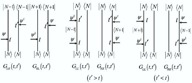
Figure 2: Double sided Feynman diagrams for the four superoperator Green’s functions. $|N\rangle$ represents a many-body state with $N$ electrons. $G_{LR}$ and $G_{RL}$ correspond to the transition from $|N\rangle$ to $|N-1\rangle$ and $|N\rangle$ to $|N+1\rangle$ state, respectively. $G_{LL}$ and $G_{RR}$ represent coherence between the two states during time interval $t$ to $t^{\prime}$.

In the long time limit, the system reaches a steady state where the current becomes independent on time and the Green’s functions only depend on the difference of their time arguments. Using Fourier transformation of $G_{\alpha\beta}(E)=\int dtG_{\alpha\beta}(t){\mbox{e}}^{iEt}$, Eq. (119) can be recast in the frequency domain as

$$I = e\sum_{ab{a^{\prime}}{b^{\prime}}}J_{ab}J_{{a^{\prime}}{b^{\prime}}}^{\ast}\int\frac{dE}{2\pi}\left[G_{RL}^{{a^{\prime}}a}(E)G_{LR}^{b{b^{\prime}}}(E)-G_{RL}^{b{b^{\prime}}}(E)G_{LR}^{{a^{\prime}}a}(E)\right].$$ (120)

As done previously, [Eqs. (101)-(103), we next assume that sub-system $B$ is a thermodynamically large, free electrons system. in this case, the current can be calculated non-perturbatively to all orders in $J$. This is derived in Appendix E. Equation (120) can then be replaced by Eq. (235)

$$I=e\sum_{a{a^{\prime}}}\int\frac{dE}{2\pi}\left[{\Sigma^{a{a^{\prime}}}_{LR}}(E)G_{RL}^{a{a^{\prime}}}(E)-{\Sigma^{a{a^{\prime}}}_{RL}}(E)G_{LR}^{a{a^{\prime}}}(E)\right]$$ (121)

where $\Sigma_{\alpha\beta}^{aa^{\prime}},\alpha,\beta=L,R$ are the elements of the self-energy matrix for sub-system $A$ due to interaction with $B$.

$$\Sigma^{a{a^{\prime}}}_{LR}(E) = i\Gamma^{A}_{aa^{\prime}}f_{B}(E),~{}~{}\Sigma^{a{a^{\prime}}}_{RL}(E)=-i\Gamma^{A}_{aa^{\prime}}[1-f_{B}(E)]$$ (122)

$$\Sigma^{a{a^{\prime}}}_{LL}(E) = -\frac{i}{2}\Gamma^{A}_{aa^{\prime}}[1-2f_{B}(E)],~{}~{}\Sigma^{a{a^{\prime}}}_{RR}(E)=\frac{i}{2}\Gamma^{A}_{aa^{\prime}}[1-2f_{B}(E)]$$ (123)

with $\Gamma^{A}_{aa^{\prime}}=2\pi\sum_{bb^{\prime}}J_{ab}J^{*}_{a^{\prime}b^{\prime}}\sigma_{B}$, where $\sigma_{B}$ is the density of states (assumed to be independent of energy) of sub-system $B$. Unlike Eq. (120), the Green’s functions in Eq. (121) now contain coupling to the leads to all orders through the self-energies. These can be evaluated by solving the matrix Dyson equation as given in Sec. VIII. Under certain approximations, Eq. (121) reduces to the LB form, Eq. (1). This is shown in Eqs. (242)-(243).

VII.4 Fluorescence induced by an electron or a hole transfer

Consider an electron transferred to a molecule attached to two leads (a molecular wire) or by an STM probe by applying an external potential. This electron may decay radiatively to one of the lower energy states by emitting a photon, before finally exiting the molecule. We denote this optical signal current-induced-fluorescence (CIF). The reverse process can occur when an electron leaves the molecule, creating a hole. An electron in one of the higher lying bound states can decay radiatively to combine with this hole. Thus the CIF signal can come either from a positively or from a negatively charged molecule where the charge is created by the interaction with external leads. This is different from ordinary (laser-induced) fluorescence (LIF) shaul-book where an electron-hole pair, created by the interaction with the laser field, recombines to produce a photon and there is no electron transfer from/to the molecule. Thus CIF involves many-body states of the molecule with different total charges whereas LIF only depends on states with the same charge.

The system is described by the Hamiltonian $\hat{H}=\hat{H}_{m}+\hat{H}_{f}+\hat{H}_{A}+\hat{H}_{B}+\hat{H}_{mf}+\hat{H}^{\prime}$ where $\hat{H}_{m}$, $\hat{H}_{f}$, $\hat{H}_{A}$ and $\hat{H}_{B}$ represent the independent molecule, radiation field, lead $A$ and lead $B$, respectively. $\hat{H}_{mf}$ is the coupling between the radiation field and the molecule

$$\hat{H}_{mf}=\hat{a}_{s}^{{\dagger}}\hat{B}+\hat{B}^{{\dagger}}\hat{a}_{s}.$$ (124)

$\hat{a}_{s}^{{\dagger}}(\hat{a}_{s})$ are, respectively, the creation (annihilation) operators for the $s$-th mode of the scattered field and $\hat{B}^{{\dagger}}(\hat{B})$ is an exciton (electron-hole pair) operator for the molecule

$$\hat{B}^{\dagger}=\sum_{i>j}\mu_{ij}\hat{\psi}^{\dagger}_{i}\hat{\psi}_{j},~{}~{}~{}\hat{B}=\sum_{i>j}\mu_{ji}\hat{\psi}^{\dagger}_{j}\hat{\psi}_{i}.$$ (125)

$\mu_{ij}$ is the dipole matrix element between the orbital $i$ and the orbital $j$.

The molecule-lead coupling $H^{\prime}$ is

$$\hat{H}^{\prime}=\sum_{x\in A,B}\sum_{i}J_{xi}\hat{\psi}_{i}^{{\dagger}}\hat{\psi}_{x}+h.c.$$ (126)

The signal is defined by the expectation value of the flux operator for the scattered photon modes,

$$S(\omega_{s},t)=\langle\frac{d}{dt}\hat{a}_{s}^{{\dagger}}\hat{a}_{s}\rangle=i\langle[\hat{H},\hat{a}_{s}^{{\dagger}}\hat{a}_{s}]\rangle.$$ (127)

The angular brackets denote the trace with respect to the full density matrix of the field+molecule+leads system

Expanding Eq. (127) perturbatively in the emitted field and in the lead-molecule coupling, the CIF signal from a negatively charged molecule can be expressed in terms of Liouville space Green’s functions. Depending on the time ordering of various superoperators corresponding to $\hat{B}$, $\hat{a}$ and $\hat{\psi}$, the density matrix evolves through different LSPs.

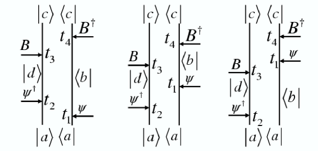
Figure 3: Three Liouville space pathways that contribute to the fluorescence from a negatively charged molecule, Eq. (128). States $|a\rangle$, $|b\rangle$, $|c\rangle$ and $|d\rangle$ denote different charge states of the molecule. Time increases from bottom to top.

For the signal to be finite, we must first prepare the molecule in one of its excited states by transferring either an electron or a hole, before bringing it down to lower excited states. This results in the cancelation of many terms in the perturbative expansion of Eq. (127). Only three LSPs (plus their complex conjugates) contribute to the signal. These can be expressed by the double sided Feynman diagrams shown in Fig. 3. The fluorescence from a negatively charged molecule is finally given by up-jeremy-prb2

$$\frac{dS_{n}}{dV}(\omega_{s})=ie\sum_{i<j}\sum_{i^{\prime}<j^{\prime}}\sum_{kl}\sigma(E_{F}+eV)J_{k}(E_{F}+eV)J_{l}(E_{F}+eV)$$ (128)

$$\times \mu_{ij}\mu_{i^{\prime}j^{\prime}}\int d\tau\int_{-\infty}^{t-\tau}d\tau_{1}\int_{-\infty}^{t}d\tau_{2}e^{-i\omega_{s}\tau}e^{-i(E_{F}+eV)(\tau_{1}-\tau_{2})}$$

$$\left[\frac{{}}{{}}G_{LL}^{ji}(t-\tau,t-\tau^{+})\left(G_{RR}^{{i^{\prime}}{j^{\prime}}}(t,t^{+})G_{RL}^{lk}(\tau_{2},\tau_{1})-G_{RL}^{l{j^{\prime}}}(\tau_{2},t)G_{RL}^{{i^{\prime}}k}(t,\tau_{1})\right)\right.$$

$$- \left.G_{RL}^{{i^{\prime}}i}(t,t-\tau)\left(G_{RL}^{jk}(t-\tau,\tau_{1})G_{RL}^{l{j^{\prime}}}(\tau_{2},t)+G_{LR}^{j{j^{\prime}}}(t-\tau,t)G_{RL}^{lk}(\tau_{2},\tau_{1})\right)\right.$$

$$+ \left.G_{RL}^{li}(\tau_{2},t-\tau)\left(G_{LR}^{j{j^{\prime}}}(t-\tau,t)G_{RL}^{{i^{\prime}}k}(t,\tau_{1})+G_{RL}^{jk}(t-\tau,\tau_{1})G_{RR}^{{i^{\prime}}{j^{\prime}}}(t,t^{+})\right)\right]$$

where $\sigma(E)=-\mbox{Im}G_{--}(E)/\pi$ is the density of states of the lead from which electron has been transferred to the molecule, evaluated at energy $E_{F}+eV$. $J_{k}(E)$ is the coupling of the $k$th molecular orbital with the state of the lead at energy $E$. A similar expression can be obtained for the signal from a positively charged moleculeup-jeremy-prb2 .

VII.5 Electroluminescence: Fluorescence induced by electron and hole transfer

Electroluminescence is the recombination of an electron and a hole, injected separately by external charge sources. This is a higher order process than described by Eq. (128), as both electron and hole are injected into the molecule from the leads. In a molecule-lead configuration, as discussed in Eqs. (124) and (126), a lowest order perturbative expression can be obtained by expanding Eq. (127) to fourth order in the left and/or right lead couplings. This contains a large number of terms. The process is simpler in the high bias limit ($V>k_{B}T$) where an electron is transferred from the left lead to the molecule while a hole is transferred from the right lead simultaneously and the reverse processes are not allowed. We then get

$$S_{EL}(\omega_{s},t) = -8\mbox{Re}\int_{-\infty}^{t}d\tau\int d\tau_{1}\int d\tau_{2}\int d\tau_{3}\int d\tau_{4}\sum_{ab}f_{a}(1-f_{b})e^{-i\epsilon_{a}(\tau_{1}-\tau_{2})}$$ (129)

$$\times e^{i\epsilon_{b}(\tau_{3}-\tau_{4})}e^{-i\omega_{s}(t-\tau)}\sum_{ijkl}J_{ia}J_{lb}J_{aj}J_{bk}$$

$$\times \langle\breve{T}\breve{B}_{L}(\tau)\breve{B}_{R}^{\dagger}(t)\breve{\psi}_{iL}^{\dagger}(\tau_{1})\breve{\psi}_{jR}(\tau_{2})\breve{\psi}_{kL}(\tau_{3})\breve{\psi}_{lR}^{\dagger}\rangle$$

where the trace is with respect to the density matrix of the free molecule. The correlation function inside the integral can be computed using the many-body states of the molecule. For a free-electron model it can be expressed as sum of the products of the Green’s functions for the molecule using Wick’s theorem.

VIII Dyson Equations for the retarded, advanced and correlation Green’s functions

In the previous section we demonstrated how various observables of the coupled system can be expressed in terms of the Green’s functions of the individual sub-systems, $G_{\alpha\beta}$. Here we show how to compute these Green’s functions with many-body (e.g. electron-electron and electron-phonon) interactions. Using the superoperator approach, a closed equation of motion (EOM) for the Green’s functions is derived directly in PTSA representation. The retarded Green’s function satisfies an independent equation (decoupled from the other Green’s functions). Nonlinear effects due to interactions with the environment are included in the self-energy which can be computed perturbatively in the interaction picture or using the generating function technique negele ; up-shaul-JCP .

The Hamiltonian of each closed system ($A$ or $B$) will be partitioned as

$$\hat{H}=\hat{H}_{0}+\hat{H}_{int}$$ (130)

where

$$\hat{H}_{0}=\sum_{x}\epsilon_{x}{\hat{\psi}^{\dagger}}_{x}{\hat{\psi}}_{x}$$ (131)

is the free-electron part where $x$ denotes the electronic degrees of freedom, e.g., orbital, spin, wavevector,etc. $\hat{H}_{int}$ represents the many-body interactions in the system. We need not specify the form of $H_{int}$ at this point.

In terms of the superoperator PTSA representation, the total Liouville operator is

$$L=L_{0}+L_{int}$$ (132)

where $L_{0}$ corresponds to $\hat{H}_{0}$

$$L_{0}=\sum_{x}\epsilon_{x}\left({\breve{\psi}^{\dagger}}_{x+}{\breve{\psi}}_{x+}-{\breve{\psi}}_{x-}{\breve{\psi}^{\dagger}}_{x-}\right)$$ (133)

and

$$L_{int} = \sqrt{2}\breve{H}_{int-}.$$ (134)

We shall construct the equation of motion (EOM) for the superoperator, $\breve{\psi}_{i\alpha}$ starting with the superoperator Heisenberg equation

$$\frac{\partial}{\partial t}{\breve{\psi}}_{i\alpha}=i[L,{\breve{\psi}}_{x\alpha}]$$ (135)

where $[L,{\breve{\psi}}_{x\alpha}]=L{\breve{\psi}}_{x\alpha}-{\breve{\psi}}_{x\alpha}L$. Substituting Eq. (132) in (135) and using the commutation rules Eq. (V) of Fermi superoperators, we get

$$\frac{\partial}{\partial t}{\breve{\psi}}_{x\alpha}=-i\epsilon_{x}{\breve{\psi}}_{x\alpha}-i\sqrt{2}[\breve{H}_{-},{\breve{\psi}}_{x\alpha}].$$ (136)

Differentiating Eq. (88) and using (136), we obtain the EOM for the Green’s functions,

$$\left(i\frac{\partial}{\partial t}-\epsilon_{x}\frac{{}}{{}}\right)G^{x{x^{\prime}}}_{\alpha\beta}(t,{t^{\prime}})=\delta_{x{x^{\prime}}}\delta_{\alpha\beta}\delta(t-{t^{\prime}})-i\sqrt{2}\langle\breve{T}[\breve{H}_{-}(t),{\breve{\psi}}_{x\alpha}(t)]{\breve{\psi}^{\dagger}}_{{x^{\prime}}\beta}({t^{\prime}})\rangle.$$ (137)

When the many-body interaction $H_{int}$ is turned off, Eq. (137) reduces to

$$\left(i\frac{\partial}{\partial t}-\epsilon_{x}\right)G^{0x{x^{\prime}}}_{\alpha\beta}(t,{t^{\prime}})=\delta_{x{x^{\prime}}}\delta_{\alpha\beta}\delta(t-{t^{\prime}}).$$ (138)

Equation (138) defines the noninteracting Green’s functions, $G_{\alpha\beta}^{0}$.

Equation (137) can be recast in the Dyson form (repeated indices are summed over).

$$\mathbf{G}(t,{t^{\prime}})=\mathbf{G}^{0}(t,{t^{\prime}})+\mathbf{G}^{0}(t,{t^{\prime}}_{1})\mathbf{\Sigma}({t^{\prime}}_{1},{t^{\prime}}_{2})\mathbf{G}({t^{\prime}}_{2},{t^{\prime}})$$ (139)

where $\mathbf{G}$ is the $2\times 2$ matrix of Greens functions, $G^{\alpha\beta}$ and the self-energy matrix $\mathbf{\Sigma}$ is defined by the equation

$$\Sigma^{x{x^{\prime}}_{1}}_{\alpha{\alpha^{\prime}}}(t,{t^{\prime}}_{1})G^{{x^{\prime}}_{1}{x^{\prime}}}_{{\alpha^{\prime}}\beta}({t^{\prime}}_{1},{t^{\prime}})=-i\sqrt{2}\langle\breve{T}[\breve{H}_{-}(t),{\breve{\psi}}_{x\alpha}(t)]{\breve{\psi}^{\dagger}}_{{x^{\prime}}\beta}({t^{\prime}})\rangle$$

$$= -i\sqrt{2}\left\langle\!\breve{T}[{\breve{H}}^{I}_{-}(t),{{\breve{\psi}^{I}}}_{x\alpha}(t)]{{\breve{\psi}}}_{{x^{\prime}}\beta}^{I{\dagger}}({t^{\prime}})\mbox{exp}\left\{-i\sqrt{2}\int_{\infty}^{t}d\tau{\breve{H}}^{I}_{-}(\tau)\right\}\right\rangle_{0}$$

$\langle\cdots\rangle_{0}$ is the trace with respect to the non-interacting density matrix of the sub-system and the time dependence is in the interaction picture with respect to $\hat{H}_{0}$.

The Dyson equation [Eq. (139)] can be written explicitly in the matrix form with

$${\bf G}=\left(\begin{array}[]{cc}G_{--}&G_{-+}\\ 0&G_{++}\end{array}\right),~{}{\bf G}^{0}=\left(\begin{array}[]{cc}G_{--}^{0}&G_{-+}^{0}\\ 0&G_{++}^{0}\end{array}\right),~{}{\bf\Sigma}=\left(\begin{array}[]{cc}\Sigma_{--}&\Sigma_{-+}\\ \Sigma_{+-}&\Sigma_{++}\end{array}\right),$$ (147)

where we have used the fact that $G^{+-}=0$, Eq. (93).

The bottom left matrix element in Eq. (147) gives

$$G^{0}_{++}\Sigma_{+-}G_{--}=0.$$ (148)

Since $G_{++}$ and $G_{--}$ do not generally vanish, Eq. (148) implies that $\Sigma_{+-}=0$. Equation (147) then gives the retarded $G_{--}$ Green’s functions thus satisfy their own Dyson equations.

$$G_{--} = G^{0}_{--}+G^{0}_{--}\Sigma_{--}G_{--}.$$ (149)

Similarly we get for the advanced Green’s function

$$G_{++}=G^{0}_{++}+G^{0}_{++}\Sigma_{++}G_{++}.$$ (150)

The correlation function $G^{-+}$ can then be expressed in terms of the retarded and the advanced Green’s functions and their self-energies

$$G_{-+} = G^{0}_{-+}+G^{0}_{-+}\Sigma_{++}G_{++}+G^{0}_{--}\left(\Sigma^{--}G_{-+}+\Sigma_{-+}G_{++}\right).$$ (151)

Keldysh had derived Eqs. (149)- (151) keldysh ; haug-jauho by starting with the coupled equations for the four Hilbert space Green’s functions in the PTBK representation (which in superoperator notation correspond to $G_{LL},G_{RR},G_{RL}$ and $G_{LR}$) and then decouple them by transforming to the PTSA representation. The superoperator approach allows us to work with the PTSA representation from the outset. The derivation is much more compact and physically-transparent.

For completeness, we present the corresponding equations for bosons in Appendix A.

IX Current-fluctuation statistics

So far we have discussed average observables, such as the total energy, change in the charge density and the current in interacting open systems. Fluctuations may be measured in electron tunneling between two conductors and electron transport through quantum junctions Rammer . Much theoreticalstatistics-theory and experimentalstatistics-experiment effort has been devoted recently to the statistical behavior of the transport through such systems. Here we do not review these works but rather give a flavor of it. More detailed derivations are given in Ref. nazarov ; two-point .

IX.1 Electron-tunneling statistics

We again consider the two interacting systems $A$ and $B$ described by the Hamiltonian, Eqs. (44) and (94). The number $k$ of electrons transferred in time $t$ can be computed by measuring the number of electrons in one of the systems at time $t=0$ and again at time $t$. The difference of the two measurements, $k$, is a fluctuating variable which changes as the measurement is repeated over the same time interval. Thus $k$ has a distribution $P(k,t)$ whose first moment gives the average current, Eq. (119). For small applied external bias, the charge transfer can reverse its course and these fluctuations may become non-negligible.

We shall compute the statistics by using the generating function associated with $P(k,t)$

$$\chi(\lambda,t)\equiv\sum_{k}\mbox{e}^{i\lambda k}P(k,t).$$ (152)

The GF is a continuous function of the parameter $\lambda$, which is conjugate to the net number of electron transfers $k$. It is convenient for computing moments of various orders by taking derivatives of GF with respect to $\lambda$. Working directly with $P(k,t)$ requires summations over the discrete variable $k$ from $-\infty$ to $\infty$. $P(k,t)$ is obtained by the inverse Fourier transform of the generating function

$$P(k,t)=\int_{0}^{2\pi}\frac{d\lambda}{2\pi}e^{-i\lambda k}\chi(\lambda,t).$$ (153)

The $n$-th moment of $P(k,t)$ is given by

$$\langle k^{n}(t)\rangle=(-i)^{n}\left.\frac{\partial}{\partial\lambda^{n}}\chi(\lambda,t)\right|_{\lambda=0}.$$ (154)

The $n$’th order cumulants are certain combinations of the moments of order $n$ and lower. The first cumulant ${\cal C}^{(1)}=\langle k(t)\rangle$ is the first moment and gives the average number of particles transferred from $A$ to $B$. The second cumulant ${\cal C}^{(2)}=\langle(k(t)-\langle k(t)\rangle)^{2}\rangle$ is the simplest measure of fluctuations of $k$ around its average value. The third cumulant ${\cal C}^{(3)}=\langle(k(t)-\langle k(t)\rangle)^{3}\rangle$ gives the skewness (asymmetry) of $P(k,t)$. For a Gaussian distribution all cumulates higher than the first two vanish. The higher cumulants thus measure the non Gaussian nature of the distribution. All cumulants of the current statistics can be computed directly by taking the derivatives of the cumulant generating function, $Z(\lambda,t)=\mbox{log}\chi(\lambda,t)$, with respect to $\lambda$. The $n$-th cumulant is given by

$$\mathcal{C}^{(n)}(t)=(-i)^{n}\left.\frac{\partial^{n}}{\partial\lambda^{n}}Z(\lambda,t)\right|_{\lambda=0}.$$ (155)

For our model, the generating function, Eq. (152), can be expressed astwo-point

$$\chi(\lambda,t)=\int_{0}^{2\pi}\frac{d\Lambda}{2\pi}\mbox{e}^{Z(\lambda,\Lambda;t)}$$ (156)

with

$$Z(\lambda,\Lambda;t)=\mbox{log}\left[\mbox{Tr}\left\{\mathcal{G}_{I}(\lambda,\Lambda,t)\rho_{0}\right\}\right]$$ (157)

and $\mathcal{G}_{I}$ is the interaction picture propagator given in Appendix F.

We shall evaluate Eq. (157) perturbatively to second order in the coupling, Eq. (94). As was done in Sec. VI, in the infinite past, the density matrix of the two systems is factorized, $\rho_{0}=\rho_{A}\oplus\rho_{B}$. The interactions are then built-in by adiabatic switching. We then express the cumulant GF, Eq. (157), in terms of the Green’s functions of systems $A$ and $B$ (see Appendix F).

$$Z(\lambda,\Lambda;t) = 2i\mbox{sin}\left(\frac{\lambda}{2}\right)\int_{-\infty}^{t}d\tau_{1}\int_{0}^{t}d\tau_{2}\left\{\theta(\tau_{1})\mathcal{F}(\lambda,\tau_{1},\tau_{2})\right.$$ (158)

$$+ \left.\theta(-\tau_{1})\left[e^{-i\Lambda}\mathcal{F}(0,\tau_{1},\tau_{2})+e^{i\Lambda}\mathcal{F}(0,\tau_{2},\tau_{1})\right]\right\}$$

with

$$\mathcal{F}(\lambda,t,{t^{\prime}}) = \sum_{a{a^{\prime}}b{{b^{\prime}}}}J_{ab}J_{{a^{\prime}}{{b^{\prime}}}}^{\ast}\left[e^{-i\frac{\lambda}{2}}G_{RL}^{{a^{\prime}}a}(t,{t^{\prime}})G_{LR}^{b,{{b^{\prime}}}}({t^{\prime}},t)-e^{i\frac{\lambda}{2}}G_{RL}^{b,{{b^{\prime}}}}(t,{t^{\prime}})G_{LR}^{{a^{\prime}}a}({t^{\prime}},t)\right].$$ (159)

All Green’s functions appearing in Eqs. (100), (109) and (159) correspond to the isolated sub-systems. These can include many-body interactions $e-e$ or $e-p$. The Green’s functions then include self-energy due to many-body interactions as shown in the previous section. The self-energy to first order in $e-e$ interactions is given in Appendix G.

IX.2 Current fluctuations: electron-transport statistics

We now consider electron transport between two leads $A$ and $B$ through a quantum system such as a molecule or a quantum dot. The total system Hamiltonian is

$$\hat{H}_{T}=\hat{H}_{A}+\hat{H}_{B}+\hat{H}_{S}+\hat{V}$$ (160)

where $\hat{H}_{A}$ and $\hat{H}_{B}$ represent Hamiltonian of two leads $A$ and $B$, and $\hat{H}_{S}$ is the system Hamiltonian. We assume a free- electron gas model for all sub-systems.

$$\hat{H}_{X}=\sum_{x\in X}\epsilon_{x}\ \hat{\psi}^{\dagger}_{x}\hat{\psi}_{x},~{}~{}~{}X=A,B,S.$$ (161)

$\hat{V}$ represents the coupling Hamiltonian between the molecule and the leads.

$$\hat{V}=\sum_{x\in A,B}J_{xi}\hat{\psi}^{\dagger}_{x}\hat{\psi}_{i}+h.c.$$ (162)

where $J_{xi}$ is the coupling between the lead ($x$) and the system ($i$) orbitals.

A simple perturbative calculation in the coupling, as was done in going from Eq. (157) to (250), will miss the non-equilibrium state of the embedded system. However, using the path-integral techniquetwo-point , the cumulant GF $Z(\lambda,\Lambda)$ can be expressed in terms of SNGF of the molecule. The final expression for the GF involves determinant of the matrix Green’s functions renormalized due to the coupling with $A$ and $B$. For long counting times, the cumulant GF is given by two-point

$$Z(\lambda,\Lambda)=\int d\omega~{}\mbox{ln}\mbox{Det}[{\bf G}^{-1}(\omega,\lambda)]$$ (163)

where the $2\times 2$ matrix ${\bf G}(\omega,\lambda)$ is obtained by solving a Dyson matrix like equation [Eq. (147)] with the following self-energy matrix

$$\Sigma^{ii^{\prime}}_{++}(\omega,\lambda) = \frac{i}{2}\Gamma^{B}_{ii^{\prime}}+\frac{i}{2}\Gamma^{A}_{ii^{\prime}}\left[e^{i\lambda}(1-f_{A}(\omega))+e^{-i\lambda}f_{A}(\omega)\right]$$ (164)

$$\Sigma^{ii^{\prime}}_{--}(\omega,\lambda) = -\frac{i}{2}\Gamma^{B}_{ii^{\prime}}-\frac{i}{2}\Gamma^{A}_{ii^{\prime}}\left[e^{i\lambda}(1-f_{a}(\omega))+e^{-i\lambda}f_{A}(\omega)\right]$$ (165)

$$\Sigma^{ii^{\prime}}_{+-}(\omega,\lambda) = -\frac{i}{2}\Gamma^{A}_{ii^{\prime}}\left[(e^{i\lambda}-1)(1-f_{A}(\omega)-(e^{-i\lambda}-1)f_{A}(\omega))\right]$$ (166)

$$\Sigma^{ii^{\prime}}_{-+}(\omega,\lambda) = -i\Gamma_{ii^{\prime}}^{B}(2f_{B}(\omega)-1)+\!\!\frac{i}{2}\Gamma_{ii^{\prime}}^{A}$$ (167)

$$\left[(e^{i\lambda}+1)(1-f_{A}(\omega))-(e^{-i\lambda}+1)f_{A}(\omega)\right]$$

here $\Gamma_{ii^{\prime}}^{X}=2\pi\sum_{x\in X}J_{xi}J_{i^{\prime}x}\delta(\omega-\epsilon_{x})$ comes from interactions with the leads. When $\lambda=0$, $\Sigma_{+-}=0$ as discussed previously (Eq. (148)), and $\Sigma_{--}$, $\Sigma_{++}$ and $\Sigma_{-+}$ reduce to ordinary retarded, advanced and correlation self-energies due to leads-molecule interaction, respectively.

X Conclusions

We have presented a superoperator Liouville space nonequilibrium Green’s function (SNGF) theory in the PTSA ($+/-$) representation for interacting open many-electron systems.

By constructing the microscopic equations of motion for superoperators in PTSA representation, the response and correlation functions are treated along the same footing in Liouville space. This is reminiscent of the MSR formulationmsr of classical statistical mechanics. The various Green’s functions of the CTPL formulation appear naturally as a consequence of a simple superoperator time ordering operation which controls the evolution of the bra and the ket of the density matrix in Liouville space. The interaction energy and the change in density matrix of individual sub-systems are directly recast in terms of the retarded, advanced and correlation Green’s functions. Electron-transfer statistics in both tunneling and transport may be formulated in terms of the SNGF. Many-body effects (such as $e-e$ interactions) can be included perturbatively through self-energies by solving the Dyson equations. A notable advantage of the PTSA representation is that since $G_{+-}=0$, the matrix Dyson equations of the other three Green’s functions are decoupled. Dyson equations for the retarded the and advanced Green’s functions are derived without computing first the matrix Dyson equation for four Keldysh Green’s functions in PTBK representation. This is because the linear transformation which results in PTSA operators can be performed at the operator level rather than on the Green’s functions or the generating function. In Liouville space we can work directly with the operators in PTSA representation. In Hilbert space (or PTBK), in contrast, one has to first compute the four (lesser, greater,time ordered, anti-time ordered) Green’s functions and only then obtain the retarded and advanced Greens functions using the matrix transformation. This is not necessary in Liouville space. The superoperator Green’s function formulation for bosons is given in Appendix A for completeness.

Appendix A SNGF for bosons

We denote the boson creation and annihilation operators by $\hat{\phi}_{i}$ and $\hat{\phi}_{i}^{\dagger}$, respectively. These satisfy the commutation relations

$$[\hat{\phi}_{i},\hat{\phi}_{j}^{\dagger}] = \delta_{ij},~{}~{}~{}[\hat{\phi}_{i},\hat{\phi}_{j}]=[\hat{\phi}_{i}^{\dagger},\hat{\phi}_{j}^{\dagger}]=0$$ (168)

the corresponding superoperators, $\breve{\phi}_{\alpha}$ and $\breve{\phi}_{\alpha}^{\dagger}$, in Liouville space are defined by Eq. (21)

$$\breve{\phi}_{L}X \equiv \hat{\phi}X,~{}~{}\breve{\phi}_{L}^{\dagger}X\equiv\hat{\phi}X$$

$$\breve{\phi}_{R}X \equiv X\hat{\phi},~{}~{}\breve{\phi}_{R}^{\dagger}X\equiv X\hat{\phi}^{\dagger}.$$ (169)

A notable difference between Eqs. (A) and (80) is the absence of the $(-1)$ factors for bosons. Boson superoperators in PTSA representation (”+” and ”-”) are defined by Eqs. (22) and satisfy commutation relations similar to Eqs. (168).

$$[\breve{\phi}_{m\alpha},\breve{\phi}_{n\beta}^{\dagger}]=\delta_{mn}\delta_{\alpha\beta},~{}[\breve{\phi}_{m\alpha},\breve{\phi}_{n\beta}]=[\breve{\phi}^{\dagger}_{m\alpha},\breve{\phi}^{\dagger}_{n\beta}]=0.$$ (170)

Using Eqs. (170) in (26) and (27), we get

$$(\hat{\phi}_{i}\hat{\phi}_{j}^{\dagger})_{-} = \frac{1}{\sqrt{2}}\left[\delta_{ij}+\breve{\phi}_{i+}\breve{\phi}_{j-}^{\dagger}+\breve{\phi}_{i-}\breve{\phi}_{j+}^{\dagger}\right]$$ (171)

$$(\hat{\phi}_{i}\hat{\phi}_{j}^{\dagger})_{+} = \frac{1}{\sqrt{2}}\left[\delta_{ij}+\breve{\phi}_{i+}\breve{\phi}_{j+}^{\dagger}+\breve{\phi}_{i-}\breve{\phi}_{j-}^{\dagger}\right].$$ (172)

The corresponding expressions for $(\hat{\phi}_{i}\hat{\phi}_{j})_{-}$ and $(\hat{\phi}_{i}\hat{\phi}_{j})_{+}$ can be obtained from Eq. (171) and (172) by simply neglecting the $\delta_{ij}$ terms inside the brackets.

In analogy to Eq. (88), the boson superoperator Green’s functions are defined as,

$$D^{mn}_{\alpha\beta}(t,{t^{\prime}})=-i\langle\breve{T}\breve{\phi}_{m\alpha}(t)\breve{\phi}_{n\beta}^{\dagger}({t^{\prime}})\rangle.$$ (173)

Using Eqs. (A) and (173), it is easy to show that $D_{+-}$, $D_{++}$ and $D_{-+}$ represent the retarded, advanced and correlation Green’s functions, and $D_{--}=0$. This gives the boson analogue of Eqs. (90)-(92).

$$D_{+-}^{ij}(t,{t^{\prime}}) = -i\theta(t-{t^{\prime}})\langle[\breve{\phi}_{i}(t),\breve{\phi}^{\dagger}_{j}({t^{\prime}})]\rangle$$ (174)

$$D_{-+}^{ij}(t,{t^{\prime}}) = i\theta({t^{\prime}}-t)\langle[\breve{\phi}_{i}(t),\breve{\phi}^{\dagger}_{j}({t^{\prime}})]\rangle$$ (175)

$$D_{++}^{ij}(t,{t^{\prime}}) = -i\langle\{\breve{\phi}_{i}(t),\breve{\phi}^{\dagger}_{j}({t^{\prime}})\}\rangle$$ (176)

$$D_{--}^{ij}(t,{t^{\prime}}) = 0.$$ (177)

Unlike Fermions, in this case $D_{--}=0$ while $D_{+-}$ represents the retarded Green’s function. This comes from the different commutation relations, Eq. (170) and (77). The different particle-statistics for bosons affects the form of the Dyson equation (Eq. (147)).

The Dyson equation for bosons, ${\bf D}=\bf{D}^{0}+\bf{D}^{0}{\bf\Xi}~{}{\bf D}$, can be derived following the same steps which lead to Eq. (147). Here

$${\bf D}=\left(\begin{array}[]{cc}0&D_{-+}\\ D_{+-}&D_{++}\end{array}\right),~{}{\bf D}^{0}=\left(\begin{array}[]{cc}0&D_{-+}^{0}\\ D_{+-}^{0}&D_{++}^{0}\end{array}\right),~{}{\bf\Xi}=\left(\begin{array}[]{cc}\Xi_{--}&\Xi_{-+}\\ \Xi_{+-}&\Xi_{++}\end{array}\right),$$ (184)

where $D^{0}$ is the Green’s function for the reference system and $\Xi$ is the self-energy due to many-body interactions.

Comparing the top right matrix elements on both sides then gives, $\Xi_{++}=0$. We finally get the boson analogues of Eqs. (148)-(151).

$$D_{+-} = D^{0}_{+-}+D_{0}^{+-}\Xi_{-+}D_{+-}$$ (185)

$$D_{-+} = D^{0}_{-+}+D_{0}^{-+}\Xi_{+-}D_{-+}$$ (186)

$$D_{++} = D^{0}_{++}\Xi_{+-}D_{-+}+D_{+-}[\Xi_{--}D_{-+}+\Xi_{-+}D_{++}].$$ (187)

These equations are decoupled and each of the Green’s functions can be computed separately. $D_{+-}$ and $D_{-+}$ represent the retarded and the advanced boson Green’s functions.

Appendix B Wick’s Theorem

Wick’s theorem states that the expectation value of the product of $n$ fermion field operators with respect to a many-body state, represented by a single Slater determinant, can be expressed as the sum of the expectation values of products of all possible pairs of operators mahan-book ; mills ; thauless ; negele . This theorem provides a practical tool for factorizing the expectation value of a time ordered product of operators to simpler quantities. Note that expectation value vanishes unless $n$ is even.

This theorem can be derived as follows. Since a single determinant represents the eigenstate of corresponds to a noninteracting Hamiltonian, $H_{0}=\sum_{ij}K_{ij}\hat{A}_{i}\hat{A}_{j}$, the expectation of a product of $n$ operators $\langle\hat{A}_{1}\hat{A}_{2}\cdots\hat{A}_{n}\rangle$ involves an integral weighted by a Gaussian operator $\sim\mbox{exp}\left(-\beta\sum_{ij}\hat{A}_{i}K_{ij}\hat{A}_{j}\right)$. Using properties of Gaussian integrals, it can be factorized as Zinn-Justin ; mills .

$$\langle\hat{A}_{1}\hat{A}_{2}\cdots\hat{A}_{n}\rangle=\sum_{P}\langle\hat{A}_{1}\hat{A}_{2}\rangle\cdots\langle\hat{A}_{n-1}\hat{A}_{n}\rangle$$ (188)

where the sum over $P$ runs over all possible pairings of $\{1,2,\cdots,n\}$, Equation (188) remains valid also for superoperators. By simply replacing all $\hat{A}_{n^{\prime}}s$ by $\breve{A}_{n\alpha},\alpha=L,R,+,-$.

$$\langle\breve{A}_{1\alpha}\breve{A}_{2\beta}\cdots\breve{A}_{n\gamma}\rangle=\sum_{P}\langle\breve{A}_{1\alpha}\breve{A}_{2\beta}\rangle\cdots\langle\breve{A}_{n-1\delta}\breve{A}_{n\gamma}\rangle.$$ (189)

Since each permutation of fermion superoperators brings a minus sign, the Wick’s theorem for fermion superoperators takes the form,

$$\langle\breve{A}_{1\alpha}\breve{A}_{2\beta}\cdots\breve{A}_{n\gamma}\rangle=\sum_{P}(-1)^{p}\langle\breve{A}_{1\alpha}\breve{A}_{2\beta}\rangle\cdots\langle\breve{A}_{n-1\delta}\breve{A}_{n\gamma}\rangle$$ (190)

where $p$ is the number of permutations required to get the right pairing. The same theorem applies to bosons by simply eliminating the $(-1)^{p}$ factors.

Appendix C Connecting the closed-time loop with the real time Green’s functions

Standard CTPL Green’s function theory is formulated in terms of four Hilbert space Green functions: time ordered $(G^{T})$, anti-time ordered $(G^{\tilde{T}})$, greater ($G^{>}$) and lesser $(G^{<})$keldysh ; haug-jauho ; mahan-book . These are defined in the Heisenberg picture as,

$$G^{T}(t_{1},t_{2}) \equiv -i\langle T\hat{\psi}(t_{1})\hat{\psi}^{\dagger}(t_{2})\rangle$$

$$= -i\theta(t_{1}-t_{2})\langle\hat{\psi}(t_{1})\hat{\psi}^{\dagger}(t_{2})\rangle+\theta(t_{2}-t_{1})\langle\hat{\psi}^{\dagger}(t_{2})\hat{\psi}(t_{1})\rangle$$

$$G^{\tilde{T}}(t_{1},t_{2}) \equiv -i\langle\tilde{T}\hat{\psi}(t_{1})\hat{\psi}^{\dagger}(t_{2})\rangle$$

$$= -i\theta(t_{2}-t_{1})\langle\psi(t_{1})\hat{\psi}^{\dagger}(t_{2})\rangle+\theta(t_{1}-t_{2})\langle\hat{\psi}^{\dagger}(t_{2})\hat{\psi}(t_{1})\rangle$$

$$G^{>}(t_{1},t_{2}) \equiv -i\langle\hat{\psi}(t_{1})\hat{\psi}^{\dagger}(t_{2})\rangle$$

$$G^{<}(t_{1},t_{2}) \equiv i\langle\hat{\psi}^{\dagger}(t_{2})\hat{\psi}(t_{1})\rangle$$ (191)

$T$ ($\tilde{T}$) is the Hilbert space time (anti-time) ordering operator, Eqs. (8) and (9).

The four Liouville space Green’s functions which appear naturally in the superoperator formulation are

$$G_{LL}(t_{1},t_{2}) = -i\langle\breve{T}\breve{\psi}_{L}(t_{1})\breve{\psi}^{\dagger}_{L}(t_{2})\rangle,~{}G_{RR}(t_{1},t_{2})=-i\langle\breve{T}\hat{\psi}_{R}(t_{1})\breve{\psi}^{\dagger}_{R}(t_{2})\rangle$$

$$G_{LR}(t_{1},t_{2}) = -i\langle\breve{T}\breve{\psi}_{L}(t_{1})\breve{\psi}^{\dagger}_{R}(t_{2})\rangle,~{}G_{RL}(t_{1},t_{2})=-i\langle\breve{T}\breve{\psi}_{R}(t_{1})\breve{\psi}^{\dagger}_{L}(t_{2})\rangle$$ (192)

To establish the connection between Eqs. (C) and (C), we shall convert the superoperators back to ordinary operators by using their definitions and anti-commutation relations. For $G_{LR}$ and $G_{RL}$, we obtain,

$$G_{LR}(t_{1},t_{2}) \equiv -i\mbox{Tr}\{\breve{T}\breve{\psi}_{L}(t_{1})\breve{\psi}^{\dagger}_{R}(t_{2})\rho\}$$ (193)

$$= -i\left[\theta(t_{1}-t_{2})\mbox{Tr}\{\breve{\psi}_{L}(t_{1})\breve{\psi}^{\dagger}_{R}(t_{2})\rho\}-\theta(t_{2}-t_{1})\mbox{Tr}\{\breve{\psi}^{\dagger}_{R}(t_{2})\breve{\psi}_{L}(t_{1})\rho\}\right]$$

$$= i\mbox{Tr}\{\hat{\psi}(t_{1})\rho\hat{\psi}^{\dagger}(t_{2})\}=i\langle\hat{\psi}^{\dagger}(t_{2})\hat{\psi}(t_{1})\rangle$$

$$= G^{<}(t_{1},t_{2})$$

$$G_{RL}(t_{1},t_{2}) \equiv -i\mbox{Tr}\{\breve{T}\breve{\psi}_{R}(t_{1})\breve{\psi}^{\dagger}_{L}(t_{2})\rho\}$$ (194)

$$= -i\left[\theta(t_{1}-t_{2})\mbox{Tr}\{\breve{\psi}_{R}(t_{1})\breve{\psi}^{\dagger}_{L}(t_{2})\rho\}-\theta(t_{2}-t_{1})\mbox{Tr}\{\breve{\psi}^{\dagger}_{L}(t_{2})\breve{\psi}_{R}(t_{1})\rho\}\right]$$

$$= i\mbox{Tr}\{\hat{\psi}^{\dagger}(t_{2})\rho\hat{\psi}(t_{1})\}=i\langle\hat{\psi}(t_{1})\hat{\psi}^{\dagger}(t_{2})\rangle$$

$$= -G^{>}(t_{1},t_{2})$$

where $\rho$ is the fully interacting many-body density matrix.

For $G_{LL}$ and $G_{RR}$ we need to distinguish between two cases,
(i). For $t_{1}>t_{2}$, we get,

$$G_{LL}(t_{1},t_{2}) \equiv -i\mbox{Tr}\{\breve{T}\breve{\psi}_{L}(t_{1})\breve{\psi}^{\dagger}_{L}(t_{2})\rho\}$$

$$= -i\mbox{Tr}\{\hat{\psi}(t_{1})\hat{\psi}^{\dagger}(t_{2})\rho\}=-i\langle\hat{\psi}(t_{1})\hat{\psi}^{\dagger}(t_{2})\rangle$$

$$G_{RR}(t_{1},t_{2}) \equiv -i\mbox{Tr}\{\breve{T}\breve{\psi}_{R}(t_{1})\breve{\psi}^{\dagger}_{R}(t_{2})\rho\}$$ (195)

$$= -i\mbox{Tr}\{\rho\hat{\psi}^{\dagger}(t_{2})\hat{\psi}(t_{1})\}=-i\langle\hat{\psi}^{\dagger}(t_{2})\hat{\psi}(t_{1})\rangle$$

(ii) For the opposite case, $t_{1}<t_{2}$, we get,

$$G_{LL}(t_{1},t_{2}) \equiv -i\mbox{Tr}\{\breve{T}\breve{\psi}_{L}(t_{1})\breve{\psi}^{\dagger}_{L}(t_{2})\rho\}$$

$$= i\mbox{Tr}\{\hat{\psi}^{\dagger}(t_{2})\hat{\psi}(t_{1})\rho\}=i\langle\hat{\psi}^{\dagger}(t_{2})\hat{\psi}(t_{1})\rangle$$

$$G_{RR}(t_{1},t_{2}) \equiv -i\mbox{Tr}\{\breve{T}\breve{\psi}_{R}(t_{1})\breve{\psi}^{\dagger}_{R}(t_{2})\rho\}$$ (196)

$$= i\mbox{Tr}\{\rho\hat{\psi}(t_{1})\hat{\psi}^{\dagger}(t_{2})\}=i\langle\hat{\psi}(t_{1})\hat{\psi}^{\dagger}(t_{2})\rangle$$

Combining Eqs. (C) and (C) we can write,

$$G_{LL}(t_{1},t_{2}) \equiv -i\mbox{Tr}\{\breve{T}\breve{\psi}_{L}(t_{1})\breve{\psi}^{\dagger}_{L}(t_{2})\rho\}$$

$$= -i\left[\theta(t_{1}-t_{2})\langle\hat{\psi}(t_{1})\hat{\psi}^{\dagger}(t_{2})\rangle-\theta(t_{2}-t_{1})\langle\hat{\psi}^{\dagger}(t_{2})\hat{\psi}(t_{1})\rangle\right]$$

$$= G^{T}(t_{1},t_{2})$$

$$G_{RR}(t_{1},t_{2}) \equiv -i\mbox{Tr}\{\breve{T}\breve{\psi}_{R}(t_{1})\breve{\psi}^{\dagger}_{R}(t_{2})\rho\}$$ (197)

$$= -i\left[\theta(t_{1}-t_{2})\langle\hat{\psi}^{\dagger}(t_{2})\hat{\psi}(t_{1})\rangle-\theta(t_{2}-t_{1})\langle\hat{\psi}(t_{1})\hat{\psi}^{\dagger}(t_{2})\rangle\right]$$

$$= -G^{\tilde{T}}(t_{1},t_{2})$$

Equations (193)-(C) show the equivalence of the Hilbert and the Liouville space Green’s functions.

Appendix D The Retarded, Advanced and Correlation Liouville-space Green’s functions

Here we show that the SNGFs $G_{--}$, $G_{++}$ and $G_{-+}$ defined as,

$$G^{ij}_{\alpha\beta}(t,{t^{\prime}})\equiv-i\langle\breve{T}\breve{\psi}_{i\alpha}(t)\breve{\psi}_{j\beta}^{{\dagger}}({t^{\prime}})\rangle$$ (198)

coincide with the retarded, advanced and correlation functions, respectively.

Starting with $G_{--}$, we expand the time ordering operator as

$$G^{ij}_{--}(t,{t^{\prime}}) = -i\langle\breve{T}\breve{\psi}_{i-}(t)\breve{\psi}_{j-}^{{\dagger}}({t^{\prime}})\rangle$$ (199)

$$= -i\left[\theta(t-{t^{\prime}})\langle\breve{\psi}_{i-}(t)\breve{\psi}_{j-}^{{\dagger}}({t^{\prime}})\rangle-\theta({t^{\prime}}-t)\langle\breve{\psi}_{j-}^{{\dagger}}({t^{\prime}})\breve{\psi}_{i-}(t)\rangle\right].$$

Substituting $\breve{\psi}_{-}=(\breve{\psi}_{L}-\breve{\psi}_{R})/\sqrt{2}$, we can write

$$\langle\breve{\psi}_{i-}(t)\breve{\psi}_{j-}^{{\dagger}}({t^{\prime}})\rangle = \frac{1}{2}[\langle(\breve{\psi}_{iL}(t)-\breve{\psi}_{iR}(t))(\breve{\psi}_{jL}^{{\dagger}}({t^{\prime}})-\breve{\psi}_{jR}^{{\dagger}}({t^{\prime}}))\rangle]$$ (200)

$$= \langle\breve{\psi}_{iL}(t)\breve{\psi}_{jL}^{{\dagger}}({t^{\prime}})\rangle+\langle\breve{\psi}_{iR}(t)\breve{\psi}_{jR}^{{\dagger}}({t^{\prime}})\rangle$$

$$- \langle\breve{\psi}_{iL}(t)\breve{\psi}_{jR}^{{\dagger}}({t^{\prime}})\rangle\!-\!\langle\breve{\psi}_{iR}(t)\breve{\psi}_{jL}^{{\dagger}}({t^{\prime}})\rangle.$$

Using the definitions of $\breve{\psi}_{L}$ and $\breve{\psi}_{R}$ [Eq. (80)], we get

$$\langle\breve{\psi}_{i-}(t)\breve{\psi}_{j-}^{{\dagger}}(t^{\prime})\rangle \equiv \langle\hat{\psi}_{i}(t)\hat{\psi}_{j}^{{\dagger}}({t^{\prime}})\rangle+\langle\hat{\psi}_{j}^{{\dagger}}({t^{\prime}})\hat{\psi}_{i}(t)\rangle=\langle\hat{\psi}_{i}(t),\hat{\psi}_{j}^{{\dagger}}({t^{\prime}})\rangle.$$ (201)

Similarly,

$$\langle\breve{\psi}_{j-}^{{\dagger}}({t^{\prime}})\breve{\psi}_{i-}(t)\rangle = \langle(\breve{\psi}_{jL}^{{\dagger}}({t^{\prime}})-\breve{\psi}_{jR}^{{\dagger}}({t^{\prime}}))(\breve{\psi}_{iL}(t)-\breve{\psi}_{iR}(t))\rangle$$ (202)

$$= \langle\breve{\psi}_{jL}^{{\dagger}}({t^{\prime}})\breve{\psi}_{iL}(t)\rangle+\langle\breve{\psi}_{jR}^{{\dagger}}({t^{\prime}})\breve{\psi}_{iR}(t)\rangle$$

$$- \langle\breve{\psi}_{jR}^{{\dagger}}({t^{\prime}})\breve{\psi}_{iL}(t)\rangle\!-\!\langle\breve{\psi}_{jL}^{{\dagger}}({t^{\prime}})\breve{\psi}_{iR}(t)\rangle$$

$$\equiv \langle\hat{\psi}_{j}^{{\dagger}}({t^{\prime}})\hat{\psi}_{i}(t)\rangle+\langle\hat{\psi}_{i}(t)\hat{\psi}_{j}^{{\dagger}}({t^{\prime}})\rangle$$

$$- \langle\hat{\psi}_{j}^{{\dagger}}({t^{\prime}})\hat{\psi}_{i}(t)\rangle\!-\!\langle\hat{\psi}_{i}(t)\hat{\psi}_{j}^{{\dagger}}({t^{\prime}})\rangle=0$$

Substituting from Eqs. (201) and (202) in (199), we get Eq.(90) for the retarded Green’s function.

Similarly,

$$G^{ij}_{++}(t,{t^{\prime}}) = -i\langle\breve{T}\breve{\psi}_{i+}(t)\breve{\psi}_{j+}^{{\dagger}}({t^{\prime}})\rangle$$ (203)

$$= -i\left[\theta(t-{t^{\prime}})\langle\breve{\psi}_{i+}(t)\breve{\psi}_{j+}^{{\dagger}}({t^{\prime}})\rangle\theta({t^{\prime}}-t)\langle\breve{\psi}_{j+}^{{\dagger}}({t^{\prime}})\breve{\psi}_{i+}(t)\rangle\right].$$

Since

$$\langle\breve{\psi}_{i+}(t)\breve{\psi}_{j+}^{{\dagger}}\rangle = \frac{1}{2}\langle(\breve{\psi}_{iL}(t)+\breve{\psi}_{iR}(t))(\breve{\psi}_{jL}^{{\dagger}}({t^{\prime}})+\breve{\psi}_{jR}^{{\dagger}}({t^{\prime}}))\rangle$$ (204)

$$= \frac{1}{2}\left[\langle\breve{\psi}_{iL}(t)\breve{\psi}_{jL}^{{\dagger}}({t^{\prime}})\rangle+\langle\breve{\psi}_{iL}(t)\breve{\psi}_{jR}^{{\dagger}}({t^{\prime}})\rangle\right.$$

$$+ \left.\langle\breve{\psi}_{iR}(t)\breve{\psi}_{jL}^{{\dagger}}({t^{\prime}})\rangle+\langle\breve{\psi}_{iR}(t)\breve{\psi}_{jR}^{{\dagger}}({t^{\prime}})\rangle\right]=0$$

and

$$\langle\breve{\psi}_{j+}^{{\dagger}}({t^{\prime}})\breve{\psi}_{i+}(t)\rangle = \frac{1}{2}\langle(\breve{\psi}_{jL}^{{\dagger}}({t^{\prime}})+\breve{\psi}_{jR}^{{\dagger}}({t^{\prime}}))(\breve{\psi}_{iL}(t)+\breve{\psi}_{iR}(t))\rangle$$ (205)

$$= \frac{1}{2}\left[\langle\breve{\psi}_{jL}^{{\dagger}}({t^{\prime}})\breve{\psi}_{iL}(t)\rangle+\langle\breve{\psi}_{jR}^{{\dagger}}({t^{\prime}})\breve{\psi}_{iL}(t)\rangle\right.$$

$$+ \left.\langle\breve{\psi}_{jL}^{{\dagger}}({t^{\prime}})\breve{\psi}_{iR}(t)\rangle+\langle\breve{\psi}_{jR}^{{\dagger}}({t^{\prime}})\breve{\psi}_{iR}(t)\rangle\right]$$

$$\equiv \langle\{\hat{\psi}_{i}(t),\hat{\psi}_{j}^{{\dagger}}({t^{\prime}})\}\rangle,$$

substituting these in Eq. (203), we get Eq.(91) for the advanced Greens function.

We next turn to $G_{-+}$

$$G^{ij}_{-+}(t,{t^{\prime}}) = -i\langle\breve{T}\breve{\psi}_{i-}(t)\breve{\psi}_{j+}^{{\dagger}}\rangle$$ (206)

$$= -i\left[\theta(t-{t^{\prime}})\langle\breve{\psi}_{i-}(t)\breve{\psi}_{j+}^{{\dagger}}({t^{\prime}})\rangle-\theta({t^{\prime}}-t)\langle\breve{\psi}_{j+}^{{\dagger}}({t^{\prime}})\breve{\psi}_{i-}(t)\rangle\right].$$

Substituting for $\breve{\psi}_{-},\breve{\psi}_{+}$ in terms of $\breve{\psi}_{L}$ and $\breve{\psi}_{R}$ gives

$$\langle\breve{\psi}_{i-}(t)\breve{\psi}_{j+}^{{\dagger}}({t^{\prime}})\rangle = \frac{1}{2}\langle(\breve{\psi}_{iL}(t)-\breve{\psi}_{iR}(t))(\breve{\psi}_{jL}^{{\dagger}}({t^{\prime}})+\breve{\psi}_{jR}^{{\dagger}}({t^{\prime}}))\rangle$$ (207)

$$= \frac{1}{2}\left[\langle\breve{\psi}_{iL}(t)\breve{\psi}_{jL}^{{\dagger}}({t^{\prime}})\rangle+\langle\breve{\psi}_{iL}(t)\breve{\psi}_{jR}^{{\dagger}}({t^{\prime}})\rangle\right.$$

$$- \left.\langle\breve{\psi}_{iR}(t)\breve{\psi}_{jL}^{{\dagger}}({t^{\prime}})\rangle-\langle\breve{\psi}_{iR}(t)\breve{\psi}_{jR}^{{\dagger}}({t^{\prime}})\rangle\right]$$

$$\equiv \frac{1}{2}\left[\langle\hat{\psi}_{i}(t)\hat{\psi}_{j}^{{\dagger}}({t^{\prime}})\rangle-\langle\hat{\psi}_{j}^{{\dagger}}({t^{\prime}})\hat{\psi}_{i}(t)\rangle\right.$$

$$+ \left.\langle\hat{\psi}_{i}(t)\hat{\psi}_{j}^{{\dagger}}({t^{\prime}})\rangle-\langle\hat{\psi}_{j}^{{\dagger}}({t^{\prime}})\hat{\psi}_{i}(t)\rangle\right]=\langle[\hat{\psi}_{i}(t),\hat{\psi}_{j}^{{\dagger}}({t^{\prime}})]\rangle$$

Similarly we can simplify the other correlation function

$$\langle\breve{\psi}^{\dagger}_{j+}({t^{\prime}})\breve{\psi}_{i-}(t)\rangle = \frac{1}{2}\langle(\breve{\psi}^{\dagger}_{jL}({t^{\prime}})+\breve{\psi}^{\dagger}_{jR}({t^{\prime}}))(\breve{\psi}_{iL}(t)-\breve{\psi}_{iR}(t))\rangle$$ (208)

$$= \frac{1}{2}\left[\langle\breve{\psi}^{\dagger}_{jL}({t^{\prime}})\breve{\psi}_{iL}(t)\rangle-\langle\breve{\psi}^{\dagger}_{jR}({t^{\prime}})\breve{\psi}_{iR}(t)\rangle\right.$$

$$+ \left.\langle\breve{\psi}^{\dagger}_{jR}({t^{\prime}})\breve{\psi}_{iL}(t)\rangle-\langle\breve{\psi}^{\dagger}_{jL}({t^{\prime}})\breve{\psi}_{iR}(t)\rangle\right]$$

$$\equiv \frac{1}{2}\left[\langle\hat{\psi}^{\dagger}_{j}({t^{\prime}})\hat{\psi}_{i}(t)\rangle-\langle\hat{\psi}_{i}({t^{\prime}})\hat{\psi}_{j}^{\dagger}(t)\rangle\right.$$

$$+ \left.\langle\hat{\psi}_{j}^{\dagger}(t)\hat{\psi}_{i}({t^{\prime}})\rangle-\langle\hat{\psi}_{i}({t^{\prime}})\hat{\psi}_{j}^{\dagger}({t^{\prime}})\rangle\right]$$

$$= -\langle[\hat{\psi}_{i}(t),\hat{\psi}^{\dagger}_{j}({t^{\prime}})]\rangle.$$

Equation (92) is obtained by substituting Eqs. (208) and (207) into (206). This function is non-causal.

Finally we consider

$$G^{ij}_{+-}(t) = -i\langle\breve{T}\breve{\psi}_{i+}(t)\breve{\psi}_{j-}^{{\dagger}}({t^{\prime}})\rangle$$ (209)

$$= -i\left[\theta(t-{t^{\prime}})\langle\breve{\psi}_{i+}(t)\breve{\psi}_{j-}^{{\dagger}}({t^{\prime}})\rangle-\theta({t^{\prime}}-t)\langle\breve{\psi}_{j-}^{{\dagger}}({t^{\prime}})\breve{\psi}_{i+}(t)\rangle\right].$$

Since

$$\langle\breve{\psi}_{i+}(t)\breve{\psi}_{j-}^{{\dagger}}({t^{\prime}})\rangle = \frac{1}{2}\langle(\breve{\psi}_{iL}(t)+\breve{\psi}_{iR}(t))(\breve{\psi}_{iL}^{{\dagger}}({t^{\prime}})-\breve{\psi}_{iR}^{{\dagger}}({t^{\prime}}))\rangle$$ (210)

$$= \frac{1}{2}\left[\langle\breve{\psi}_{iL}(t)\breve{\psi}_{jL}^{{\dagger}}({t^{\prime}})\rangle-\langle\breve{\psi}_{iL}(t)\breve{\psi}_{jR}^{{\dagger}}({t^{\prime}})\rangle\right.$$

$$+ \left.\langle\breve{\psi}_{iR}(t)\breve{\psi}_{jL}^{{\dagger}}({t^{\prime}})\rangle-\langle\breve{\psi}_{iR}(t)\breve{\psi}_{jR}^{{\dagger}}({t^{\prime}})\rangle\right]$$

$$\equiv \frac{1}{2}\left[\langle\hat{\psi}_{i}(t)\hat{\psi}_{j}^{{\dagger}}({t^{\prime}})\rangle+\langle\hat{\psi}_{j}^{{\dagger}}({t^{\prime}})\hat{\psi}_{i}(t)\rangle\right.$$

$$- \left.\langle\hat{\psi}_{i}(t)\hat{\psi}_{j}^{{\dagger}}({t^{\prime}})\rangle-\langle\hat{\psi}_{j}^{{\dagger}}({t^{\prime}})\hat{\psi}_{i}(t)\rangle\right]=0.$$

Similarly it can be shown that $\langle\breve{\psi}_{j-}^{{\dagger}}(t)\breve{\psi}_{i+}({t^{\prime}})\rangle=0$. Equation (93) follows from Eq. (209).

Appendix E Currents through Molecular junctions with free-electron leads

In Sec. VII.3 we assumed a small quantum system $A$ coupled to an infinite system $B$. This corresponds to molecular wire or STM experiments where a single molecule (or a quantum dot), the ”system”, is coupled to two metal leads which are large compared to the system. In this appendix we show how by adopting a free electron model of the leads, the current can be calculated nonperturbatively in the coupling with the leads. The total Hamiltonian is

$$H_{T}=H_{S}+H_{A}+H_{B}+V.$$ (211)

$H_{A}$ and $H_{B}$ are the free leads Hamiltonians given in Eq. (161). $V$ is the coupling of the system with the leads, Eq. (162). The system Hamiltonian in this case is quite general and can include electron-electron and/or electron-phonon interactions.

$$H_{S} = \sum_{i}\epsilon_{i}\hat{\psi}_{i}^{{\dagger}}\hat{\psi}_{i}+\sum_{ijkl}V_{ijkl}\hat{\psi}_{i}^{{\dagger}}\hat{\psi}_{j}^{{\dagger}}\hat{\psi}_{k}\psi_{l}+\sum_{m}\Omega_{m}\hat{\phi}_{m}^{{\dagger}}\hat{\phi}_{m}+\sum_{ijm}\lambda_{ij}^{m}\hat{\psi}_{i}^{{\dagger}}\hat{\psi}_{j}(\hat{\phi}_{m}^{{\dagger}}+\hat{\phi}_{m})$$

where the fermion operators $\hat{\psi}^{{\dagger}}(\hat{\psi})$ satisfy the anti-commutation relations, Eq. 77. Indices $(i,j,k,l)$ and $(m,n)$ represent the system electronic states and system phonon states respectively. $\epsilon_{i}$ and $\Omega_{m}$ are corresponding energies. $\lambda_{ij}$ and $V_{ijkl}$ are the $e-p$ and $e-e$ interaction matrix elements. $\hat{\phi}_{m}^{{\dagger}}(\hat{\phi}_{m})$ are phonon creation (annihilation) operator for the $m$-th normal mode, with frequency $\Omega_{m}$. These operators $\hat{\phi}$ satisfy the boson commutation relations, Eqs. (168).

The current from lead $A$ (left) to the system is defined as the rate of change of the total charge of the lead,

$$I(t)\equiv\sum_{l}\frac{d}{dt}\langle\hat{N}_{A}\rangle=i\sum_{l}\langle[H_{T},\hat{N}_{A}(t)]\rangle$$ (213)

where $\hat{N}_{A}=e\sum_{a}\psi^{{\dagger}}_{a}\psi_{a}$ is the number operator for the left lead. We substitute the Hamiltonian and calculate the commutator. $\hat{N}_{A}$ commutes with all terms in the Hamiltonian, except the interaction $V$, Eq. (162). We obtain

$$I(t)=-2e\mbox{Im}\left\{\sum_{ia}J_{ia}\langle\psi^{{\dagger}}_{i}(t)\psi_{a}(t)\rangle_{T}\right\}$$ (214)

where $\langle\cdots\rangle_{T}$ is the trace with respect to the total (system+leads) density matrix. A Similar expression can be written for the current from the right lead $B$ to the system by changing $a$ with $b$ in Eq. (214). At steady state the two currents are same.

The Liouville space Green’s functions are connected with their Hilbert space counterparts in Appendix C. The current, Eq. (214), can be expressed in terms of the Liouville space Greens function as

$$I(t)=2e\mbox{Re}\{J_{ia}(t)G_{LR}^{ai}(t,t)\}.$$ (215)

In Eq. (215), the Green’s function $G_{LR}^{ai}$ is defined in the joint leads+system space. We compute $G_{LR}(t,{t^{\prime}})$ and then set $t={t^{\prime}}$. In a recent work Rabani rabani has used a numerical path-integral approach to directly compute the Green’s function $G_{LR}$ (hence the current).

We shall compute this Green’s function using the equation of motion technique. To that end, we construct the equation of motion for $\breve{\psi}_{a\alpha}(t)(\alpha=L,R)$ using the Heisenberg equation for superoperators

$$\frac{\partial}{\partial t}\breve{\psi}_{a\alpha}(t)=i\sqrt{2}[\breve{H}_{-},\breve{\psi}_{a\alpha}(t)]$$ (216)

where on the right-hand side

$$[\breve{H}_{-},\breve{\psi}_{a\alpha}(t)]=\breve{H}_{-}\breve{\psi}_{a\alpha}(t)-\breve{\psi}_{a\alpha}(t)\breve{H}_{-}$$ (217)

and $\breve{H}_{-}=(\breve{H}_{L}-\breve{H}_{R})/\sqrt{2}$ can be expressed in terms of $\breve{\psi}_{L}$ and $\breve{\psi}_{R}$ using Eq. (III). Equation (216) then gives

$$i\frac{\partial}{\partial t}\breve{\psi}_{a\alpha}(t)=\epsilon_{a}\breve{\psi}_{a\alpha}(t)+\sum_{i}J_{ai}^{*}(t)\breve{\psi}_{i\alpha}(t).$$ (218)

Taking the time derivative of Eq. (88) with $x=l,y=i$ and $\mu=\alpha,\nu=\beta$, we get

$$i\frac{\partial}{\partial t}G_{\alpha\beta}^{ai}(t,{t^{\prime}})=\delta(t-{t^{\prime}})\delta_{\alpha\beta}\delta_{ai}+\langle\mathcal{T}\left(\frac{\partial}{\partial t}\hat{\psi}_{a\alpha}(t)\right)\hat{\psi}^{\dagger}_{i\beta}({t^{\prime}})\rangle.$$ (219)

The $\delta(t-{t^{\prime}})$ factor comes from the time derivation of the step function (which originates from $\breve{T}$) and the Kronecker delta functions result from the commutation relations, Eqs. (V). Using Eq. (218) in (219) we get

$$(i\frac{\partial}{\partial t}-\epsilon_{a})G_{\alpha\beta}^{ai}(t,{t^{\prime}})=\sum_{j}J_{aj}^{*}(t)G_{\alpha\beta}^{ji}(t,{t^{\prime}})$$ (220)

Note that $a\neq i$, since they belong to different regions of the total system. Thus the first term on the r.h.s. in Eq. (219) does not contribute in this case. To zeroth order in lead-system interaction, the Green’s function for the leads is defined as,

$$(i\frac{\partial}{\partial t}-\epsilon_{a})g_{\alpha\beta}^{aa^{\prime}}(t,{t^{\prime}})=\delta(t-{t^{\prime}})\delta_{\alpha\beta}\delta_{aa^{\prime}}.$$ (221)

Substituting this in Eq. (220), we can write

$$G_{\alpha\beta}^{ai}(t,{t^{\prime}})=g_{\alpha{\beta^{\prime}}}^{aa^{\prime}}(t,t_{1})J^{*}_{a^{\prime}{i^{\prime}}}(t_{1})G^{i{i^{\prime}}}_{{\beta^{\prime}}\beta}(t_{1},{t^{\prime}}).$$ (222)

For $G_{LR}$ this gives,

$$G_{LR}^{ai}(t,{t^{\prime}}) = J^{*}_{a^{\prime}{i^{\prime}}}(t_{1})\left(g_{LL}^{aa^{\prime}}(t,t_{1})G_{LR}^{{i^{\prime}}i}(t_{1},{t^{\prime}})+g_{LR}^{aa^{\prime}}(t,t_{1})G_{RR}^{{i^{\prime}}i}(t_{1},{t^{\prime}})\right).$$ (223)

The current, Eq. (215), then becomes

$$I(t)\!\! = \!\!2e\mbox{Re}\!\!\!\sum_{i{i^{\prime}}aa^{\prime}{\beta^{\prime}}}\!\!\int dt_{1}J_{ia}J_{ja^{\prime}}^{*}g_{L{\beta^{\prime}}}^{aa^{\prime}}(t,t_{1})G_{{\beta^{\prime}}R}^{ji}(t_{1},t).$$ (224)

We define the Fourier transform

$$G(E_{1},E_{2})=\int dt_{1}dt_{2}\mbox{e}^{-i(E_{1}t_{1}+E_{2}t_{2})}G(t_{1},t_{2}).$$ (225)

Equation (224) then gives

$$I(t) = 2e\mbox{Re}\sum_{ijaa^{\prime}{\beta^{\prime}}}\int d\tilde{E}J_{ai}J^{*}_{a^{\prime}{i^{\prime}}}\mbox{e}^{i(E_{1}+E_{3})t}g_{L{\beta^{\prime}}}^{ll^{\prime}}(E_{1},E_{2})G_{{\beta^{\prime}}R}^{ji}(-E_{2},E_{3})$$ (226)

where $d\tilde{E}=dE_{1}dE_{2}dE_{3}/(2\pi)^{5}$. Using the relations up-shaul-JCP

$$G_{--} = G_{LL}-G_{LR},~{}G_{++}=G_{LL}+G_{RL},~{}G_{LL}+G_{RL}=G_{RR}+G_{LR}$$ (227)

equation (226) can be transformed to

$$I(t) = 2e\mbox{Re}\sum_{ijaa^{\prime}}\int d\tilde{E}J_{ai}J^{*}_{a^{\prime}{i^{\prime}}}\mbox{e}^{i(E_{1}+E_{3})t}$$ (228)

$$\times \left[g_{aa^{\prime}}^{--}(E_{1},E_{2})G_{LR}^{ji}(-E_{2},E_{3})+g^{a^{\prime}}_{LR}(E_{1},E_{2})G^{ij}_{++}(-E_{2},E_{3})\right].$$

We next compute the steady-state current ($t\to\infty$). Integrating both sides over time, we obtain the (time-independent) current

$$I = 2e\mbox{Re}\sum_{ijaa^{\prime}}J_{ai}J^{*}_{a^{\prime}{i^{\prime}}}\int\frac{dE_{1}dE_{2}dE_{3}}{(2\pi)^{3}}\left[g^{aa^{\prime}}_{--}(E_{1},E_{2})G_{LR}^{ji}(-E_{2},-E_{1})\right.$$ (229)

$$\quad\quad\quad+\left.g^{aa^{\prime}}_{LR}(E_{1},E_{2})G^{ij}_{++}(-E_{2},-E_{1})\right].$$

At steady state, since the one-particle Green’s functions only depend on the difference of their arguments, we can make the change of variables, $E_{1}-E_{2}=E$. Equation (229) then gives

$$I = 2e\mbox{Re}\sum_{i{i^{\prime}}aa^{\prime}}J_{ai}J^{*}_{a^{\prime}{i^{\prime}}}\int\frac{dE}{2\pi}\left(g_{--}^{aa^{\prime}}(E)G_{LR}^{{i^{\prime}}i}(E)+g_{LR}^{aa^{\prime}}(E)G_{++}^{{i^{\prime}}i}(E)\right).$$ (230)

Using the relations, ${G^{ij}_{--}}^{\ast}=G^{ji}_{++}$ and ${G_{LR}^{ij}}^{\ast}=-G_{LR}^{ji}$, we can write Eq. (230) as

$$I = e\sum_{i{i^{\prime}}aa^{\prime}}J_{ia}J_{a^{\prime}{i^{\prime}}}^{*}\int\frac{dE}{2\pi}\left[G_{LR}^{i{i^{\prime}}}(E)\{2i\mbox{Im}g^{aa^{\prime}}_{--}(E)\}-g_{LR}^{ll^{\prime}}(E)\{2i\mbox{Im}G_{i{i^{\prime}}}^{--}(E)\}\right].$$

From Eqs. (227), we have $-2i\mbox{Im}\{G_{--}\}=G_{LR}+G_{RL}$. Substituting this in Eq. (E), we get

$$I = e\sum_{i{i^{\prime}}aa^{\prime}}J_{ia}J_{a^{\prime}{i^{\prime}}}^{*}\int\frac{dE}{2\pi}\left[g_{LR}^{aa^{\prime}}(E)G_{RL}^{i{i^{\prime}}}(E)-g_{RL}^{aa^{\prime}}(E)G_{LR}^{i{i^{\prime}}}(E)\right].$$ (232)

Since the leads are assumed to be in equilibrium, we can express their Green’s functions using the fluctuation-dissipation relations

$$g_{LR}^{aa^{\prime}}(E) = 2\pi if_{A}(E)\sigma_{aa}(E)\delta_{aa^{\prime}}$$

$$g_{RL}^{aa^{\prime}}(E) = 2\pi i(1-f_{A}(E))\sigma_{aa}(E)\delta_{aa^{\prime}}$$ (233)

where $f_{A}(E)=[1+\mbox{exp}\{\beta(E-\mu_{A})\}]^{-1}$ and $\sigma_{aa^{\prime}}(E)=-(1/\pi)\mbox{Im}\{G_{--}(E)\}$ are the Fermi function and the density of states (DOS) for the left lead with chemical potential $\mu_{A}$. The current then becomes

$$I=ie\sum_{i{i^{\prime}}}\Gamma_{i{i^{\prime}}}^{A}\int\frac{dE}{2\pi}\left[f_{A}(E)G_{RL}^{i{i^{\prime}}}(E)-(1-f_{A}(E))G_{LR}^{i{i^{\prime}}}(E)\right]$$ (234)

where $\Gamma_{i{i^{\prime}}}^{A}=\sum_{aa^{\prime}}2\pi J_{ia}J_{{i^{\prime}}a^{\prime}}^{*}\sigma_{aa^{\prime}}$ and the DOS of the leads is assumed to be energy independent in the relevant energy range (chemical potential difference of the two leads). This can also be expressed in terms of the self-energies due to the interaction with the left lead $\Sigma_{\alpha\beta}$

$$I=e\sum_{i{i^{\prime}}}\int\frac{dE}{2\pi}\left[{\Sigma^{i{i^{\prime}}}_{LR}}(E)G_{RL}^{i{i^{\prime}}}(E)-{\Sigma^{i{i^{\prime}}}_{RL}}(E)G_{LR}^{i{i^{\prime}}}(E)\right]$$ (235)

where $\Sigma^{i{i^{\prime}}}_{LR}(E)=\Gamma_{ii^{\prime}}^{A}f_{A}(E)$ and $\Sigma^{i{i^{\prime}}}_{RL}(E)=\Gamma_{ii^{\prime}}^{A}[1-f_{A}(E)]$. Equation (235) is same as Eq. (121).

A similar expression can be obtained for the current from lead $B$ to the system by replacing $a$ with $b$ in Eq. (234).

$$I^{\prime}=ie\sum_{i{i^{\prime}}}\Gamma_{i{i^{\prime}}}^{B}\int\frac{dE}{2\pi}\left[f_{B}(E)G_{RL}^{i{i^{\prime}}}(E)-(1-f_{B}(E))G_{LR}^{i{i^{\prime}}}(E)\right].$$ (236)

At steady state $I=-I^{\prime}$ and the steady state current $I_{s}$ can be written as, $I_{s}=xI-(1-x)I^{\prime}$ for any value of $x$. Using Eqs. (234) and (236), we obtain

$$I_{s} = ie\sum_{i{i^{\prime}}}\int\frac{dE}{2\pi}\left\{[xf_{A}(E)\Gamma^{A}_{i{i^{\prime}}}-(1-x)f_{B}(E)\Gamma^{B}_{i{i^{\prime}}}]\right.$$

$$\times \left.(G_{RL}^{i{i^{\prime}}}(E)+G_{LR}^{i{i^{\prime}}}(E))-[x\Gamma^{A}_{i{i^{\prime}}}-(1-x)\Gamma^{B}_{i{i^{\prime}}}]G_{LR}^{i{i^{\prime}}}(E)\right\}$$

This can be simplified further by using, $-2i\mbox{Im}\{G_{--}\}=G_{LR}+G_{RL}$, to get

$$I_{s} = -ie\sum_{i{i^{\prime}}}\int\frac{dE}{2\pi}\left\{2i[xf_{A}(E)\Gamma^{A}_{i{i^{\prime}}}-(1-x)f_{B}(E)\Gamma^{B}_{i{i^{\prime}}}]\right.$$ (238)

$$\times \left.\mbox{Im}G^{--}_{i{i^{\prime}}}(E)+[x\Gamma^{A}_{i{i^{\prime}}}-(1-x)\Gamma^{B}_{i{i^{\prime}}}]G_{LR}^{i{i^{\prime}}}(E)\right\}.$$

This is the general exact formal expression for the current that includes both the left and right lead properties. As a check let us assume no external bias and set, $f_{A}=f_{B}=f$. Equation (238) then reduces to

$$I_{s} = -ie\sum_{i{i^{\prime}}}\int\frac{dE}{2\pi}[x\Gamma^{A}_{i{i^{\prime}}}-(1-x)\Gamma^{B}_{i{i^{\prime}}}][2if(E)\mbox{Im}G_{--}^{i{i^{\prime}}}(E)+G_{LR}^{i{i^{\prime}}}(E)]$$ (239)

At equilibrium, $G_{LR}(E)=-2if(E)\mbox{Im}G_{--}(E)$ (which is the FD theorem)haug-jauho , and $I_{s}$ vanishes, as it should.

Assuming that the coupling elements are real, $\Gamma_{ij}=\Gamma_{ji}$, Eq. (236) can be expressed in a simple form in terms of retarded and correlation Greens functions as

$$I=ie\sum_{i{i^{\prime}}}\Gamma_{i{i^{\prime}}}^{A}\int\frac{dE}{2\pi}\left[i(1-2f_{A}(E))\mbox{Im}G_{--}^{i{i^{\prime}}}(E)+\frac{1}{2}G^{-+}_{i{i^{\prime}}}(E)\!\right].$$ (240)

When the left and the right lead-system couplings satisfy $\Gamma_{i{i^{\prime}}}^{A}=\lambda\Gamma_{i{i^{\prime}}}^{B}$, the current $I_{s}$ can be expressed solely in terms of the imaginary part of the retarded Greens function. Choosing $x=1/(1+\lambda)$ in Eq. (238) gives

$$I_{s}=2e\sum_{i{i^{\prime}}}\frac{\Gamma^{A}_{i{i^{\prime}}}\Gamma^{B}_{i{i^{\prime}}}}{\Gamma^{A}_{i{i^{\prime}}}+\Gamma^{B}_{i{i^{\prime}}}}\mbox{Im}\int\frac{dE}{2\pi}(f_{A}(E)-f_{B}(E))G_{--}^{i{i^{\prime}}}(E).$$ (241)

This can be recast as,

$$I_{s}=2e\int\frac{dE}{2\pi}(f_{B}(E)-f_{A}(E))\sum_{i{i^{\prime}}}|S_{i{i^{\prime}}}(E)|^{2}.$$ (242)

where

$$|S_{ii^{\prime}}(E)|^{2}=\frac{\Gamma^{A}_{i{i^{\prime}}}\Gamma^{B}_{i{i^{\prime}}}}{\Gamma^{A}_{i{i^{\prime}}}+\Gamma^{B}_{i{i^{\prime}}}}\mbox{Im}G^{ii^{\prime}}_{--}(E)$$ (243)

Equation (242) has the LB form given in Eq. (1). From Eq. (241) it is easy to see that the steady state current vanishes when the external bias is turned off ($f_{A}=f_{B}$) or one of the leads is disconnected (so that $\Gamma^{A}=0$ or $\Gamma^{B}=0$). We note that the condition $\Gamma_{i{i^{\prime}}}^{A}=\lambda\Gamma_{i{i^{\prime}}}^{B}$ trivially holds when the leads are coupled to a single system orbital.

When the system is modeled as non-interacting electron system and the system-lead interactions are small, we can use

$$G^{i{i^{\prime}}}_{--}(E)=\delta_{i{i^{\prime}}}\frac{1}{E-\epsilon_{i}+i\eta}$$ (244)

where $\epsilon_{i}$ is the single electron energy. Substituting this in Eq. (241) then gives

$$I_{s}=2e\sum_{i}\!\frac{\Gamma_{ii}^{A}\Gamma_{ii}^{B}}{\Gamma_{ii}^{A}+\Gamma_{ii}^{B}}(f_{B}(\epsilon_{i})-f_{A}(\epsilon_{i})).$$ (245)

This coincide with the quantum master equation appraochup-max-shaulPRB1 .

In general, the steady state current is given by Eq. (235) which involves the Green’s functions $G_{LR}$ and $G_{RL}$. These can be calculated by solving the matrix Dyson equation self-consistently. When the coupling to the left and the right leads are proportional, $\Gamma^{A}=\lambda\Gamma^{B}$, Eq. (235) can be recast in the simpler form, Eq. (241), which involves properties of both the leads. Finally, when the molecule is modeled as noninteracting electron system, the current is simply the sum of independent contributions from each orbital (Eq. (245)).

Appendix F Connecting Eq. (157) with Eq. (158)

The time evolution operator ${\cal G}^{I}$ in Eq. (157) is given bytwo-point

$$\mathcal{G}_{I}(\lambda,\Lambda,t)=\breve{T}\mbox{exp}\left\{-i\sqrt{2}\int_{-\infty}^{t}d\tau\breve{V}^{I}_{-}(\gamma_{\alpha}(t);\tau)\right\}$$ (246)

where

$$\breve{V}_{-}(\gamma_{\alpha}(t);\tau) = \frac{1}{\sqrt{2}}[\breve{V}_{L}(\gamma_{L}(\tau);\tau)-\breve{V}_{R}(\gamma_{R}(\tau);\tau)]$$ (247)

$$\breve{V}_{\alpha}(\gamma_{\alpha}(t);t) = e^{-i\gamma_{\alpha}(t)}\breve{H}_{AB\alpha}^{\prime}(t)+h.c.$$ (248)

Note that for $\gamma_{\alpha}(t)=0$, $\mathcal{G}_{I}(\gamma_{\alpha}(t);t,t_{0})$ is simply the time evolution operator for the density matrix. The time dependence in Eq. (246) is due to the interaction picture with respect to Hamiltonian $\hat{H}_{0}=\hat{H}_{A}+\hat{H}_{B}$ and $\breve{H}_{AB\alpha}^{\prime}=\sum_{ab}J_{ab}({\hat{\psi}^{\dagger}}_{a}{\hat{\psi}}_{b})_{\alpha}$. The parameters $\gamma_{\alpha}(t)\equiv\theta(t)\gamma_{\alpha}$ with

$$\gamma_{L}=\Gamma+\frac{\gamma}{2},~{}~{}~{}~{}\gamma_{R}=\Gamma-\frac{\gamma}{2}.$$ (249)

$\gamma_{\alpha}$ is an auxiliary field in Liouville space which modifies the tunneling between the two sub-systems and acts differently on the ket and the bra of the density matrix. A similar approach was used up-shaul-JCP to extend the well known GW equations hedin ; onida-RMP ; gunnarsson-Review to non-equilibrium systems. The GF, $Z(\lambda,\Lambda,t)$ can be computed perturbatively in the tunneling matrix elements, $J_{AB}$. Since $\langle\hat{V}_{-}(\tau)\rangle=0$ (particle conservation in individual noninteracting systems),to lowest (second) order we obtain,

$$Z(\lambda,\Lambda,t)=-\int_{t_{0}}^{t}\int_{t_{0}}^{t}d\tau_{1}d\tau_{2}\langle\breve{T}\breve{V}_{-}(\gamma_{\alpha}(\tau_{1});\tau_{1})\breve{V}_{-}(\gamma_{\alpha}(\tau_{2});\tau_{2})\rangle$$ (250)

By substituting Eqs. (247) and (248) for $\breve{V}_{-}(\tau)$ and noting that $\langle\breve{H}_{AB\alpha}(\tau_{1})\breve{H}_{AB\beta}(\tau_{2})\rangle$ vanishes (particle conservation; trace is over the product states), we obtain Eq. (158).

Appendix G Self-energy for Electron-electron interactions

The $e-e$ interactions in the system are represented by the Hamiltonian.

$$\hat{H}_{int}=\sum_{ijkl}V_{ijkl}{\hat{\psi}^{\dagger}}_{i}{\hat{\psi}^{\dagger}}_{j}{\hat{\psi}}_{k}{\hat{\psi}}_{l}$$ (251)

with

$$V_{ijkl}=e\int\int dxdx^{\prime}\varphi_{i}^{*}(x)\varphi_{k}(x)\frac{1}{|x-x^{\prime}|}\varphi_{j}^{*}(x^{\prime})\varphi_{l}(x^{\prime})$$ (252)

and $\varphi_{i}$ is the basis set wavefunction at site $i$. Note that $V_{ijkl}=V_{jilk}$. In this section all the superoperator indices shall correspond to $+$ and $-$ operators.

The corresponding superoperator in the PTSA representation is given by

$$L_{int} = \sum_{ijkl}\sum_{\alpha\beta{\alpha^{\prime}}{\beta^{\prime}}}V_{ijkl}\left[{{\breve{\psi}^{\dagger}}}_{i\alpha}{{\breve{\psi}^{\dagger}}}_{j\beta}{{\breve{\psi}}}_{k{{\alpha^{\prime}}}}\breve{\psi}_{l{\beta^{\prime}}}+(-1)^{p+1}\breve{\psi}_{l{\beta^{\prime}}}\breve{\psi}_{k{\alpha^{\prime}}}\breve{\psi}^{\dagger}_{j\beta}\breve{\psi}^{\dagger}_{i\alpha}\right]$$ (253)

where $p$ is the number of ”minus” operators in the second term inside the bracket. Substituting this in Eq. (VIII) and expanding the exponential, the self-energy $\Sigma_{\alpha\beta}$ can be evaluated perturbatively in $e-e$ interaction, $V_{ijkl}$. To first order we get,

$$\Sigma^{ij}_{\alpha\beta}(t,{t^{\prime}})\! = \!\!\frac{-i}{2}\delta(t-{t^{\prime}})\!\!\sum_{{\alpha^{\prime}}{\beta^{\prime}}}\sum_{i^{\prime}k^{\prime}}W^{{i^{\prime}}i{k^{\prime}}j}_{{\alpha^{\prime}}\alpha{\beta^{\prime}}\beta}G^{{k^{\prime}}{i^{\prime}}}_{{\beta^{\prime}}{\alpha^{\prime}}}(t,t)$$ (254)

where

$$W^{{i^{\prime}}i{k^{\prime}}j}_{{\kappa^{\prime}}\kappa{\eta^{\prime}}\eta}=(V_{{i^{\prime}}i{k^{\prime}}j}-V_{i{i^{\prime}}{k^{\prime}}j})[1+(-1)^{p+1}]$$ (255)

with $p$ the number of ”minus” indices ${k^{\prime}},\kappa,\eta^{\prime}\eta$ of $W$. The electron-phonon self-energy can be calculated similarlyup-shaul-prb1 .

Appendix H Self-energy for a molecular-wire connected to free electron leads

Here we compute the Green’s functions for a molecule attached to two leads. The leads are assumed to be non-interacting electron system which remain at equilibrium with their respective chemical potentials. We also ignore the many-body interactions in the molecule. For this model, the interaction with the leads can be computed exactly within the Green’s function approach. The total Hamiltonian is given by, Eq. (160).

The EOM for the Green’s function $G^{ij}_{\alpha\beta}(t,{t^{\prime}})$ is obtained as in Eq. (219).

$$i\frac{\partial}{\partial t}G_{\alpha\beta}^{ij}=\delta(t-{t^{\prime}})\delta_{\alpha\beta}\delta_{ij}+\left\langle\breve{T}\frac{\partial}{\partial t}\breve{\psi}_{i\alpha}(t)\breve{\psi}^{\dagger}_{j\beta}({t^{\prime}})\right\rangle.$$ (256)

Using the EOM for superoperator $\breve{\psi}_{i\alpha}$ in the Heisenberg picture

$$i\frac{\partial}{\partial t}\breve{\psi}_{i\alpha}(t)=\epsilon_{i}\breve{\psi}_{i\alpha}(t)+\sum_{x\in A,B}J_{ix}\breve{\psi}_{x\alpha},$$ (257)

Eq. (256) can be expressed as (repeated indices are summed over),

$$\left(i\frac{\partial}{\partial t}-\epsilon_{i}\right)G_{\alpha\beta}^{ij}(t,{t^{\prime}})=\delta(t-{t^{\prime}})\delta_{\alpha\beta}\delta_{ij}+\Sigma_{\alpha{\beta^{\prime}}}^{ik}(t{t^{\prime}}_{1})G_{{\beta^{\prime}}\beta}^{kj}({t^{\prime}}_{1},{t^{\prime}}).$$ (258)

In Eq. (258), the self-energy ($\sigma$) due to molecule-lead couplings is defined as

$$\Sigma_{\alpha{\beta^{\prime}}}^{ik}(t{t^{\prime}}_{1})G_{{\beta^{\prime}}\beta}^{kj}({t^{\prime}}_{1},{t^{\prime}})=-i\sum_{x\in A,B}J_{ix}\left\langle\breve{T}\breve{\psi}_{x\alpha}(t)\breve{\psi}_{j\beta}^{\dagger}({t^{\prime}})\right\rangle.$$ (259)

Note that in Eq. (259) on the rhs the self-energy is given in terms of the cross-correlation Green’s function defined in the joint space of the lead and the molecule. We wish to express it in using the Green’s functions of the individual systems non-perturbatively. For this purpose, starting from the EOM for the lead superoperator $\breve{\psi}_{x\alpha}$, we construct the EOM for the joint Green’s function.

$$\left(i\frac{\partial}{\partial t}-\epsilon_{x}\right)G_{\alpha\beta}^{xj}(t,{t^{\prime}})=\sum_{k}J_{xk}G_{\alpha\beta}^{kj}(t,{t^{\prime}}).$$ (260)

This can also be recast as

$$G_{\alpha\beta}^{xj}(t,{t^{\prime}})=\sum_{k{x^{\prime}}}g_{\alpha{\beta^{\prime}}}^{x{x^{\prime}}}(t,{t^{\prime}}_{1})J_{{x^{\prime}}k}G_{{\beta^{\prime}}\beta}^{kj}({t^{\prime}}_{1},{t^{\prime}})$$ (261)

where $g_{\alpha\beta}^{x{x^{\prime}}}$ is the Green’s function for the free (in absence of the molecule) leads defined as,

$$\left(i\frac{\partial}{\partial t}-\epsilon_{x}\right)g_{\alpha\beta}^{x{x^{\prime}}}(t,{t^{\prime}})=\delta(t-{t^{\prime}})\delta_{\alpha\beta}\delta_{x{x^{\prime}}}.$$ (262)

Substituting Eq. (261) in (259), and using the identity $G_{\alpha{\beta^{\prime}}}^{ij}(t,{t^{\prime}}_{1})G_{{\beta^{\prime}}\beta}^{jk}({t^{\prime}}_{1},{t^{\prime}})=\delta_{\alpha\beta}\delta_{ik}$ , the self-energy can be written as

$$\Sigma_{\alpha\beta}^{ij}(t,{t^{\prime}})=-i\sum_{x,{x^{\prime}}}J_{ix}g_{\alpha\beta}^{x{x^{\prime}}}(t,{t^{\prime}})J_{{x^{\prime}}j}.$$ (263)

Since $g_{\alpha\beta}^{x{x^{\prime}}}$ is the Green’s function for the independent leads, it is diagonal in $x,{x^{\prime}}$, $g_{\alpha\beta}^{x{x^{\prime}}}=\delta_{x{x^{\prime}}}g_{\alpha\beta}$. Transforming to frequency domain, Eq. (263) then gives,

$$\Sigma_{\alpha\beta}^{ij}(E)=-i\sum_{x\in A,B}J_{ix}g_{\alpha\beta}^{xx}(E)J_{xj}.$$ (264)

The self-energy can be finally obtained using the expressions for the lead Green’s functions $g_{LR}$ and $g_{RL}$ given in Eqs. (E). The Green’s function $g_{LL}=g_{--}+g_{LR}$ [Eq. (227)], where $g_{--}$ can be obtained from Eq. (103), and $g_{RR}=g_{LL}+g_{RL}-g_{LR}$ [Eq. (227)]. This defines all elements of the self-energy matrix which appears in Eqs. (121) and (235).

References

- (1) J. Schwinger, J. Math. Phys. 2 (1961) 407-432.
- (2) L. V. Keldysh, Sov. Phys. J. 20 (1965) 1018-1026.
- (3) D. C. Langreth, in ”Linear and Non-linear transport in Solids”, edited by J. T. Devreese and V. E. van Doren, 17 of Nato Advanced Study Institute, Series B: Physics, Plenum, New York, (1976).
- (4) J. Rammer, ”Quantum Theory of Non-equilibrium States”, Cambridge University Press, Ney York, (2007).
- (5) L. P. Kadanoff and G. Byam, ”Quantum Statistical Mechanics”, Bejamin, New york, (1962).
- (6) A. M. Zagoskin, ”Quantum Theory of Many-Body Systems. Techniques and Applications”, Springer-Verlag, New York, (1998).
- (7) G.D. Mahan, Many Particle Physics, Plenum Press, New York (1993), P. 95.
- (8) H. Haug and A-P. Jauho, ”Quantum Kinetics in Transport and Optics of Semiconductors”, Springer-Verlag, Berlin, Heidelberg, (1996), p. 59.
- (9) J. Rammer and H. Smith, Rev. Mod. Phys. 58 (1986) 323-359.
- (10) S. Datta, Electronic Transport in Mesoscopic Systems, Cambridge University Press, Cambridge, (1997) Ch. 8.
- (11) H. Arai and T. Fujikawa, Phys. Rev. B 72 (2005) 075102- 075117.
- (12) C. Caroli, D. Lederer-Rozenblatt, B. Roulet, and D. Saint-James, Phys. Rev. B 8 (1973) 4552-4569.
- (13) T. Fujikawa and H. Arai, Chem. Phys. Lett. 368 (2003) 147-152.
- (14) K.-c. Chou, Z.-b. Su, B.-l. Hao and L. Yu, Phys. Rep. 118 (1985) 1-131.
- (15) E. Wang, U. Heinz, Phys. Rev. D 66 (2002) 025008.
- (16) R. Mills, Propagators for many-particle systems; an elementary treatment, New York, Gordon and Breach (1969).
- (17) S. Mukamel, Phys. Rev. A 77 (2008) 023801; Phys. Rev. A., 76 (2007) 021803.
- (18) B.-l. Hao, Physica 109A (1981) 221-236.
- (19) W. Wai-Yong, L. Z.-Heng, Su Z.-Bin and H. Bai-Lin, Chinese Physics 3 (1983) 813-820.
- (20) S. Mukamel, Principles of Nonlinear Optical Spectroscopy, Oxford University Press, New York, (1995), P. 45.
- (21) U. Harbola and S. Mukamel, J. Chem. Phys. 124 (2006) 044106-044117.
- (22) L. Hedin, Phys. Rev. 139 (1965) 796-823; J. Phys.: Condens. Matter 11 (1999) R489-R528.
- (23) G. Onida, L. Reining, and A. Rubio, Rev. Mod. Phys. 74 (2002) 601-659.
- (24) F. Aryasetiawan and O. Gunnarsson, Rep. Prog. Phys. 61 (1998) 237-312.
- (25) U. Harbola, J. Maddox and S. Mukamel, Phy. Rev. B 73 (2006) 205404-205418.
- (26) U. Harbola, J. Maddox and S. Mukamel, Phy. Rev. B 73 (2006) 075211-075229.
- (27) V. Chernyak, N. Wang, S. Mukamel, Phys. Rep. 263 (1995) 213-309.
- (28) S. Mukamel, Phys. Rev. E 68 (2003) 021111.
- (29) A. E. Cohen and S. Mukamel, J. Phys. Chem. A 107 (2003) 3633-3638.
- (30) A. E. Cohen and S. Mukamel, Phys. Rev. Lett. 91 (2003) 233202-233205.
- (31) U. Harbola and S. Mukamel, Phys. Rev. A 70 (2004) 052506-052521.
- (32) S. Mukamel, Phys. Rev. A 71 (2005) 024503-024506.
- (33) R. V. Leeuwen, Int. J. Mod. Phys. B 15 (2001) 1969-2023.
- (34) W. Kohn and J. L. Sham, Phys. Rev. 140 (1965) 1133-1138.
- (35) P. Hohenberg and W. Kohn, Phys. Rev. 136 (1964) 864-871.
- (36) R. A. Marcus, Rev. Mod. Phys. 65 (1993) 599 - 610.
- (37) ”Electron Transfer–From Isolated Molecules To Biomolecules”, edts. J. Jortner and M. Bixon, Adv. Chem. Phys. John Wiley and Sons Ltd, 106 (1999)
- (38) Q. Wu and T. Van Voorhis, J. Chem. Phys. 25 (2006) 164105.
- (39) C. L. Cheng, J. S. Evans and T. Van Voorhis, Phys. Rev. B 74 (2006) 155112.
- (40) J. Rammer, A. L. Shelankov and J. Wabnig, Phys. Rev. B 70 (2004) 115327; A. Shelankov and J. Rammer, Europhys. Lett. 63 (2003) 485-491; L. S. Levitov, H. Lee and G. B. Lesovik, J. Math. Phys. 37 (1996) 4845.
- (41) M, Buttiker, Science 313 (2006) 1587; C. Texier and M. Buttiker, Phys. Rev. B 62 (2000) 7454-7458; T. Fujisawa, T. Hayashi, R. Tomita, and Y. Hirayama, Science 312 (2006) 1634; H. Kiesel, A. Renz and F. Hasselbach, Nature 418 (2002) 392.
- (42) R. J. Glauber, Phys. Rev. 131 (1963) 2766; T. Jeltes, J. M. McNamara, W. Hogervorst, W. Vassen, V. Krachmalnicoff, M. Schellekens, A. Perrin, H. Chang, D. Boiron, A. Aspect and C. I. Westbrook, Nature 445 (2007) 402.
- (43) R. J. Glauber, ”Quantum Theory of Optical Coherence”, Wiley-VCH Verlag GmbH & Co. (2007).
- (44) S. Mukamel, Phys. Rev. A, 68 (2003) 063821.
- (45) T. la C. Jansen and S. Mukamel, J. Chem. Phys. 119 (2003) 7979.
- (46) R. Landauer, IBM J. Res. Dev. 1 (1957) 223; M. B ttiker, Phys. Rev. Lett. 57 (1986) 1761.
- (47) J. Bardeen, Phys. Rev. Lett. 6 (1961) 57-59.
- (48) J. Tersoff and D. R. Hamann, Phys. Rev. Lett. 50 (1983) 1998-2001; Phys. Rev. B 31 (1985) 805-815.
- (49) C. Marx, U. Harbola and S. Mukamel, Phys. Rev. A, 77 (2008) 022110.
- (50) W. Ho, J. Chem. Phys. 117 (2002) 11033-11061.
- (51) C. Caroli, R. Combescot, P. Noziér, and D. S.-James, J. Phys. C 5 (1972) 21.
- (52) Faraday Discuss. 117 (2000) 277-290; N. Lorente, M. Persson, L. J. Lauhon, and W. Ho, Phys. Rev. Lett. 86 (2001) 2593-2596.
- (53) N. Lorente and M. Persson, Phys. Rev. Lett. 85 (2000) 2997.
- (54) J. M. Blanco, C. Gonzalez, P. Jelinek, J. Ortega, F. Flores and R. Perez, Phys. Rev. B 70 (2004) 085405-085414.
- (55) Y. Asai, Phys. Rev. Lett. 93 (2004) 246102-246105; 94 (2005) 099901E-099902 ; T. Frederiksen, M. Brandbyge, N. Lorente, and A.-P. Jauho, Phys. Rev. Lett. 93 (2004) 256601-26603; S. Tikhodeev, M. Natario, K. Makoshi, T. Mii, and H. Ueba, Surf. Sci. 493 (2001) 63-70.
- (56) M. Galperin, M. A. Ratner, and A. Nitzan, J. Chem. Phys. 121 (2004) 11965-11980.
- (57) Y. Karzazi and J. Cornil and J. L. Br/’edas, J. Am. Chem. Soc. 123 (2001) 10076-10084; Nanotechnology 14 (2003) 165-171; Cornil, J.; Karzazi, Y.; Bredas, J. L. J. Am. Chem. Soc.; (Communication); 124(14) (2002) 3516-3517.
- (58) S. N. Rashkeev, M. Di Ventra, and S. T. Pantelides, Phys. Rev. B 66 (2002) 033301.
- (59) J. B. Maddox, U. Harbola, K. Mayoral and S. Mukamel, J. Phys. Chem. C. 111 (2007) 9516-9522.
- (60) S. W. Wu, N. Ogawa and W. Ho, 312 (2006) 1362-1365.
- (61) P. C. Martin, E. D. Siggia and H. A. Rose, Phys. Rev. A 8 (1973) 423-442.
- (62) M. Wagnmer, Phys. Rev. B 44 (1991) 6104-6117.
- (63) U. Fano, Phys. Rev. 131 (1963) 259-268.
- (64) R. Zwanzig, Nonequilibrium Statistical Mechanics, Oxford University Press, New York, (2001).
- (65) A. B.-Reuven, Adv. Chem. Phys. 33 (1975) 235-293.
- (66) M. Schmutz, Z. Phys. B 30 (1978) 97.
- (67) M. A. Slifkin, Charge transfer interactions of biomolecules, London, New York, Academic Press, (1971).
- (68) E. M. Lifshitz and L. P. pitaevskii, Physical Kinetics, Pergamon, Oxford, (1981).
- (69) M. A. van Eijck, R. Kobes and C. G. van Weert, Phys. Rev. D 50 (1994) 4097-4109.
- (70) A. D. McLachlan, Proc. R. Soc. London, Ser. A 271 (1963) 387-401; 274 (1963) 80-90.
- (71) A. J. Stone, The Theory of Intermolecular Forces, Clarendon Press, Oxford, 1996.
- (72) J. P. Perdew, R. G. Parr, M. Levy, J. R. Balduz Jr., Phys. Rev. Lett. 49 (1982) 1691.
- (73) J. P. Perdew in Density Functional Methods in Physics, R. M. Dreizler, da providencia, J., Plenum, New York (1985), p 265.
- (74) M. Cohen, and A. Wasserman, Isr. J. Chem. 43 (2003) 219; A. J. Stat. Phys. 125 (2006) 1125; J. Phys. Chem. A 111 (2007) 2229.
- (75) R. Parr and W. Yang, ”Density Functional Theory of Atoms and Molecules”, Oxford University Press: New York, (1989).
- (76) N. D. Mermin, Phys. Rev. A 137 (1965)
- (77) J. Rammer, Quantum Transport Theory, Westview Press, USA (2004).
- (78) A. Braggio, J. Kőnig and R. Fazio, Phys. Rev. Lett. 96 (2006) 026805; M. Esposito, U. Harbola and S. Mukamel, Phys. Rev. B 75 (2007) 155316; L. S. Levitov and M. Reznikov, Phys. Rev. B 70 (2004) 115305; J. Rammer, A. L. Shelenkov and J. Wabing, Phys. Rev. B 70 (2004) 115327; D. A. Begrets and Yu. V. Nazarov, Phys. Rev. B 67 (2003) 085316.
- (79) T. Fujisawa, T. Hayashi, R. Tomita and Y. Hiriyama, Science 312 (2006) 1634; T. Fujisawa, T. Hayashi, Y. Hiriyama and H. D. Cheong, Appl. Phys. Lett. 84 (2004) 2343; W. Lu, Z. Ji, L. Pfeiffer, K. W. West and A. J. Rimberg, Nature 423 (2003) 422; J. Bylander, T. Duty, P. Delsing, Nature 434 (2005) 361.
- (80) M. Kindermann, Y. V. Nazarov, and C. W. J. Beenakker, Phys. Rev. Lett. 90, (2003) 246805.
- (81) M. Esposito, U. Harbola and S. Mukamel, Rev. Mod. Phys. 2008 (To be submitted).
- (82) D. J. Thouless, ”The Quantum Mechanics of Many-Body Systems”, Academic Press, Inc. (1961).
- (83) J. Negele and H. Orland, ”Quantum Many Particle Physics”, Westview Press, Boulder, Colorado, (1998).
- (84) J. Zinn-Justin, ”Path Integrals in Quantum Mechanics”, Oxford University Press, New York, 2005.
- (85) L. M hlbacher and Eran Rabani, ”Real-time path integral approach to nonequilibrium many-body quantum system”, Cond-mat/arXiv:0707.0956
- (86) U. Harbola, M. Esposito and S. Mukamel, Phys. Rev. B 74 (2006) 235309.