Covariant versions of Margolus-Levitin Theorem
Abstract
The Margolus-Levitin Theorem is a limitation on the minimal evolving time of a quantum system from its initial state to its orthogonal state. It also supplies a bound on the maximal operations or events can occur within a volume of spacetime. We compare Margolus-Levitin Theorem with other form of limitation on minimal evolving time, and present covariant versions of Margolus-Levitin Theorem in special and general relativity respectively. The relation among entropy bound, maximum information flow and computational limit are discussed, by applying the covariant versions of Margolus-Levitin Theorem.
pacs:
03.67.Lx, 04.60.-m, 03.65.-wI Introduction
In the view of quantum theory, the time-energy uncertainty relation
is interpreted as the limitation of how fast can a quantum system
evolve from its initial state to an distinguishable state,
equivalently, to an orthogonal state. In this relation,
can be understood as the minimal evolving time between two distinct
states of the quantum system. The time-energy uncertainty relation
indicates the minimal
evolving time is constrained by the energy spread of the system.
Recently, Margolus and Levitin gave an other interpretation of
Heisenberg principle. In their proposition, the average energy
instead of the energy spread of the system is constraining the
minimal evolving time . The Margolus-Levitin Theorem has several advantages.
For an isolated system the average energy is conserved while the
energy spread can be arbitrary. More over, for complicated system
the average energy is easy to determined while the energy spread
require more information or assumption from the system. As a result,
the Margolus-Levitin Theorem is widely used on a series of
topicsML ; lloyd1 ; lloyd2 ; lloyd3 ; lloyd4 ; lloyd5 ; Zych ; Ng ; Xiao .
Some direct applications of Margolus-Levitin Theorem are taken to evaluate the speed of
ultimate quantum computerlloyd1 , the total operations
performed by the universelloyd2 and the accuracy of measuring
the spacetime geometrylloyd3 ; Ng ; Xiao . Following Margolus-Levitin Theorem , once
the average energy of the system is determined, the minimal evolving
time between two distinct states is also determined. A quantum
computer with every operation performed as quickly as the minimal
evolving time has reached the maximum speed of the average energy.
If we perceive the universe as such an quantum computer, as we
already know the energy density and the age scale of the universe,
we can work out the total operations performed by the universe from
its beginning. This lead us to the third application, what is the
accuracy of measuring the spacetime geometry? A spacetime region can
be viewed as a container filled with operations or events. The
accuracy of spacetime measurement depends on density and
distribution of the operations or events. Accordingly, these
applications of Margolus-Levitin Theorem are using abstract or concrete models, including
quantum mechanical, cosmological, and quantum gravitational ones.
Since the Margolus-Levitin Theorem is quantum mechanical, and is deduced in pure state
system with a non-interacting hamiltonian. What is the validity of
Margolus-Levitin Theorem on these applications?
In some previous work, Lloyd and his cooperators have discussed the
extension of Margolus-Levitin Theorem in composite systems, mixed states, and entangled
systemslloyd4 ; lloyd5 . They showed the Margolus-Levitin Theorem is still valid to
estimate the minimal evolving time of these systems. Also, Lloyd
have given out an attempting generalization of Margolus-Levitin Theorem in gravitational
systems. What’s more, Zelinski and Zych have made modification on
Margolus-Levitin Theorem to evaluate some specific systems more preciselyZych . In
this letter we will discuss these generalizations and modifications.
We will show that the generalized form of Margolus-Levitin Theorem proposed by Lloyd has
failed to apply on some systems, i.e. the radiation dominating era
of the universe. Lloyd’s form is covariant but not the correct
covariant version for Margolus-Levitin Theorem. Thus we will give out our covariant
versions of Margolus-Levitin Theorem, which correctly evaluate all relativistic systems
and gravitational systems.
This paper will be organized as follow. in Sec. II, we revisit the Margolus-Levitin Theorem and its extension in frame of quantum mechanics. In Sec. III, the Margolus-Levitin Theorem on mixed state, composite system and entanglement were discussed. It shows that Margolus-Levitin Theorem as an fundamental limit on still works on these systems. In Sec. IV, we focus on constructing a covariant form of Margolus-Levitin Theorem when the special relativistic effect was taken into account. Since we still don’t have a complete quantum theory of gravity, we can’t obtain a similar theorem in general relativity from the fundamental level. We analyze this problem in a semiclassical way in Sec. V, and get a similar conclusion with Sec. IV. After that, the application of the formula of covariant quantum limits of computation is discussed in Sec. VI. We discuss the close relation among entropy bound, maximum information flow and ultimate computational limit, it is found that the order of magnitude of maximum logical operations of a system during the amount of time of communicating from one side to the other is no less than the entropy of the system , or the amount of information that the system can store. Remarkably, this naturally gives a physical interpretation of the inequality in the first set of hypotheses in fmw . Discussions and conclusions will be made in Sec. VII.
II The Margolus-Levitin Theorem
The Margolus-Levitin Theorem states a quantum system with energy expectation value above its ground state energy, could transform from one original state to its orthogonal state in the time , where ML . Firstly, let us consider an arbitrary quantum system could be decomposed as superposition of its energy eigenstates,
| (1) |
where is the th eigenstates of the system with energy . We assumed the system have a discrete spectrum and the ground state energy is set zero. By quantum mechanics, after a time interval , the system will transform to,
| (2) |
Then we set the inner product to be,
| (3) |
In order to obtain the minimal value of evolving time, we use inequality , which is valid for ,Then,
| (4) | ||||
The system reaches its orthogonal state while we set .Then we finally obtain , where is the expectation value of the system energy(The ground state energy does not account for , which only add a global phase factor in equations). Some examples which saturate the inequality have been found in ML , so gives a upper bound of how fast can a system transform to its orthogonal state. This is the main conclusion of Margolus-Levitin Theorem . If we use a different inequality such as:
| (5) |
where , then we obtain a more complicate form of the estimationZych :
| (6) |
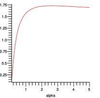

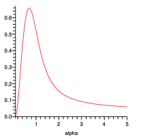
Here is the ground state energy, and denotes the expectation value on initial state. This new estimation will get a higher bound than Margolus-Levitin Theorem on in some special caseZych , but we are not able to obtain a new bound with a constant , which limit more strictly than Margolus-Levitin Theorem universally, as in Fig. 1. On the other hand, the physical interpretation of the expression with is obscure. The bound of Eq. (6) is more meaningful in mathematics than in physics. However, Margolus-Levitin Theorem relates the minimal evolving time to the average energy of the system, which offers a relatively clear physical picture. As a result, we still perceive Margolus-Levitin Theorem as a fine bound of in this letter, and all our generalizations are based on Margolus-Levitin Theorem .
III Margolus-Levitin Theorem on mixed state, composite system and entanglement
In quantum mechanics, mixed states, composite systems and entangled systems are always focused on as well as pure states, single and non-entangled ones. Some previous worklloyd4 ; lloyd5 shows that Margolus-Levitin Theorem as an fundamental limit on has its successful applications on these systems. Consider a general state , and we assume can be decomposed with orthogonal energy eigenstates,
| (7) |
Here can be viewed as a mixed state or a pure state, depending what value takes. Time translation denoted by an unitary operator transform to ,
| (8) |
A widely used function fidelity is devoted to discriminate orthogonality on mixed states. When we set to confirm the orthogonality, it is easy to obtain:
| (9) |
is energy value of (Here the Hamiltonian is assumed to be diagonal). We can easily see that fidelity coincide with the inner product between initial and final states, while is specialized to a pure state. Further deduction gives out , and is the energy expectation value of the mixed state. Noting that we have not taken interacting Hamiltonian in our consideration yet. Directly, this generalization on mixed state lead us to investigate the self consistency of Margolus-Levitin Theorem on all kinds of composite quantum systems. For example, a mixed state can be composed by several pure states(), or, a pure state can be represented as directed product of several pure states, etc. A question is asked, what is relationship between the minimal time to orthogonal state of the system and of the th subsystem? It is answered that in the latter case, is no longer limited by , but,
| (10) |
Here is the energy expectation value of the th subsystem,
unless one of the subsystems has all the energy of the
systemlloyd4 . It does mean a composite system may reach its
orthogonal state with longer time than single ones with the same
average energy. However, the total operations performed by the
system should independent of its architecturelloyd4 . In one
second, a system with average energy would perform as most
operations, which is the exact summation
of maximum operations performed by the subsystems(). This is another advantage
of Margolus-Levitin Theorem, the operation rate of any system/subsystem limited by Margolus-Levitin Theorem is proportional to its energy expectation value, which is a fine
extensive variable. In contrast, the operation rate limited by
energy spread lloyd4 ; lloyd1 or Eq. (6) is
not additive generally, which could cause some severe problem.
So far we have discussed the minimal time to orthogonal state of a non-entangled system with a free Hamiltonian. Although the entangled case or interacting case of Margolus-Levitin Theorem is difficult to formulated, some testing calculation lloyd4 implies a composite system with entanglement-generating Hamiltonian are capable to operate with a rate closer to the Margolus-Levitin Theorem bound than without it. The differences are dependent on the dominance of interacting, while Margolus-Levitin Theorem is still valid in these cases.
IV A special relativistic form of Margolus-Levitin Theorem
Margolus-Levitin Theorem enable us to evaluate how many operations or events can be discriminated at most of a 4-D space-time system, within a section of its history. The result should be invariant under any physical transformation of the observer. But apparently, the above form of the bound is not invariant in relativity. Assuming a system with average energy could be reported with operations at most in time , in a rest frame . Now there is another observer in frame , watching is moving along the axis with velocity , with an average energy for a time interval in the same history, where . The new limitation of operations in frame is . This paradox does not even exist in special relativity. Accordingly, a moving clock ticks slower than a same static clock with a rate for time dilatation effect. And the quantities of the ticks or operations detected from the clock is independent of observers for causality. Margolus and Levitin has already give a testing formML of the bound of operation quantities detected in , in a special relativity view, which is . The inner product of 4-momentum and 4-translation guarantees Lorentz invariance of the bound. And this result is easily achieved by replacing quantum field theory of quantum mechanics in deduction. For simplicity we focus on a state composed by massive particlesweinberg ,
| (11) |
The indexes mean the -th eigenstate of is occupied by an -th kind of particle with 4-momentum and spin and so on. In quantum field theory, a time translation is perceived as a trivial Lorentz transformation of the coordinates by , as
| (12) |
With a Lorentz boost, the state transforms to,
| (13) |
Then the time translation becomes spacetime translation after the boost,
| (14) | ||||
Here, is a Lorentz transformation to the coordinate, is the Lorentz transformation belonging to the little group, and furnish a representation of the little group. More details can be found in weinberg . Then the form of inner product between the two states becomes relevant to the Lorentz boost,
| (15) | ||||
We still use inequality to obtain the special relativistic form of Margolus-Levitin Theorem,
| (16) | ||||
Where , , and is the expectation value of 4-momentum of the system. A quick analysis gives the bound of minimal evolving time of orthogonal state of the system,
| (17) |
The physical picture of this inequality is confusing. Because time is not a Lorentz invariant variable, it is not wise for us to seek a relativistic invariant form of minimal evolving time between orthogonal states of the system. Although a system evolving for a time interval in the rest frame , could be described undergoing a dilated time in the moving frame , the bound of quantities of operations or events in the same history is still invariant,
| (18) |
Where we denote and by and
for simplification, and we denote the upper bound of quantities
of operations by . This result is inevitable, since
is an direct covariant representation of in the rest frame
. If the 3-components of are all zero—-it means the system
is relative static to observer—-the upper bound
degenerates to the original form . It shows Margolus-Levitin Theorem still works
on systems static to observer, and evaluating a covariant bound of
is more practical than a covariant bound of . Hence
we should seek a generalized form of Margolus-Levitin Theorem to give the bound of
of a system other than .
As long as the system is simple, it is possible to get the 4-momentum and 4-translation of the system, and to make an inner product. However in practice, it is hard to define 4-momentum and 4-translation of some complex system such as fluids or radiations. In most theoretical analysis the enery-momentum tensor is more general than 4-momentum, so a generalized form of Margolus-Levitin Theorem should take as an component of estimation of the bound. Apparently, an observer with unit timelike 4-velocity in Minkowski spacetime will obtain an energy current density wald , as measuring a fluid with energy momentum tensor , and the current density satisfies . By using Gauss’s law, we can get the conservation of energy. Thus we can straightforwardly replace in Eq. (18) by (here a constant is omitted) and then we get,
| (19) |
The equivalence between Eq. (19) and Margolus-Levitin Theorem can be proved by setting weinberg2 , noting that a 3-volume contracts by a factor under boost of Lorentz transformation. Since is 4-translation of the system, is not an arbitrary observer’s 4-velocity, but the 4-velocities of observers at rest with respect to the system. This ensures the bound of the system with same history is not depending on different observers. The covariance of the generalized form is obvious. is a scalar and is an invariant 4-volume unit in a flat background. The operational capacity of a system is now determined by and the most quantities of operations or events can be detected is proportional to the size of the 4-volume of the system. It must be emphasized that the non-negative requires the system obeying the weak energy condition,
| (20) |
Though in some theory, system with matter violating weak energy
condition is not unstable and is able to evolve from its initial
state to an orthogonal state to perform operations, the validity of
Margolus-Levitin Theorem on these systems is still to be evaluated carefully. We assert
that our estimations of upper bound of quantities of operations are
following the weak energy condition.
The generalized form of Margolus-Levitin Theorem has a direct application on cosmology. Consider a flat universe with constant above -1, which describes the massive dust dominant era and radiation dominant era of the universe. We have Friedmann equations with a flat metric:
| (21) |
| (22) |
| (23) |
Here is the energy-momentum tensor of the dominating matter, is pressure density, is energy density and we have . Resolving Friedmann equations, we obtain,
| (24) |
We will omit the constant for following discussion. Substituting Eq. (21), Eq. (24) and the representation of into Eq. (19), and take the apparent horizon as the physical bound of our universe, we obtain,
| (25) |
The result has the same order of Lloyd’s result lloyd2 . According to our result, the bounds of the quantities of events detected in our universe vary from different expanding history. This is different with Lloyd’s result, since his deduction has omitted the expanding details of the universe. The result depending on can be explained that different expanding history dilute the energy density of the universe with different rate, while the expanding horizon contains more operational units from outside with different rate. Then the form of upper bound of the total events in the observed universe is different among different expanding eras, while it always scales similar to the area of the horizon. It is consistent with and complementary to the Bekenstein boundlloyd3 . Any appliance of Eq. (19) on the matter dominating era is not successful, e.g. the cosmological constant. Since Margolus-Levitin Theorem is discussing average energy above the ground state, it is not reasonable applying Margolus-Levitin Theorem on cosmological constant, which could be interpreted to vacuum energy.
V A general relativistic form of Margolus-Levitin Theorem
In the special relativity, we find that the upper bound of
operations is associate with a conserved quantity of energy.
However, in general relativity, there is not a notion of the local
stress-energy tensor of the gravitational field. Nevertheless, for
asymptotically flat spacetimes, conserved quantity of energy
associated with asymptotic symmetries has been well defined at
spatial and null infinitywald2 . Since there are lots of
approaches to define conserved energy, we assert that our result may
not be unique in the most general contexts.
In general relativity, the energy properties of matter also represented by a energy momentum tensor , and the energy momentum current is still:
| (26) |
The local energy density of matter as measured by a given observer with unit timelike four-velocity is well defined bywald :
| (27) |
So, locally the energy in a cell with spacial volume is , the maximum logical operations in the cell within proper time of the observer is:
| (28) |
The form is very similar with Eq. (19). One would expect Eq. (19) may be still valid in general relativisty. However, the condition does not lead to a global conservation law in general relativity( is generally non-zero, not like in special relativity). There is no conserved total energy in general relativity, unless there is a Killing vector in the spacetime, i.e.,. In this case , and the conserved total energy associated with the Killing field on a spacelike Cauchy hypersurface can be defined as,
| (29) |
where denotes the unit normal vector to . Here the spacetime have been foliated by Cauchy hypersurface which is parameterized by a global time function , then the metric can be write in ADM form,
| (30) |
is called the lapse function which measures the difference
between the coordinate time and proper time on curves
normal to the Cauchy hypersurfaces , is called the
shift vector which measures the difference between a spatial
point and the point one would reach if instead of following
from one Cauchy hypersurface to the next one followed a curve
tangent to the normal , and is the intrinsic metric
induced on the hypersurface by , The timelike normal
defines the local flow of time in .
The energy defined in Eq. (29) is just the total energy on observed by an observer with 4-velocity , the maximum logical operations of over proper time is bounded by
| (31) |
Alternatively, from the definition of energy density in Eq. (27), we suspect the maximal logical operations the fluid over time would have the form,
| (32) |
This definition of energy coincides with the definition in (29) when the Killing vector satisfies,
| (33) |
This means Eq. (32) is valid when the spacetime manifold have symmetries which can generate time killing vectors normal to . We can write as the proper volume element of spacetime 4-volume , then
| (34) |
Obviously, this form of Margolus-Levitin Theorem is covariant and consistent with Eq.
(19) in special relativity. So far we know little about
quantum gravity, we are not able to give a deduction of the
generalized form of Margolus-Levitin Theorem from the fundamental level. However, the
picture of the generalized form is proved to be compatible with
quantum mechanics and general relativity.
Consider a fluid with energy momentum tensor spreads in a spacetime region with gravitational field . We assume the distribution of the fluid is static and spherical symmetric, and the size of the system is , the bound of the integral is omitted for simplification. Then the upper bound of quantities of operations is represented by,
| (35) |
Here is the area of a unit 2-sphere, and . It seems there is no difference between Eq.
(35) and the special relativistic form. However, the
gravitational effect has already been included in Eq. (35).
The Margolus-Levitin Theorem relates the minimal evolving time to the average energy of
the system, while the average energy here should be the sum of
energy not gained from gravity and energy gained from gravity. Here
the energy not gained from gravity is ,and the energy gained from
gravity is gravitation . is below zero, and is lowering
down the total average energy. This implicates that the system
performs operations slower in gravitational field. While since a
system in gravitation field has the same average energy with an
other system without considering gravity, as measured by an observer
from infinity, they have the same bound of quantities of operations,
even one of them performs slower. This can be explained from the
other aspect as following. An operation unit of the system takes
at infinity to reach its orthogonal state. Because of the
time dilation effect of general relativity, if we put the unit into
gravitational field, the minimal evolving time will expands to
as measured by observers at
infinity. However, the physical size of system in gravitational
field is times larger than the size as measured by
observers at infinity. If the outside of the static spherical system
is vacuum, we can obtain . As a result, the
system in gravitational field could maximally perform as many
operations as the system with the same average energy out of
gravitational field. Negative binding energy keeps the bound fixed
although the operation units are slowed and the amount of operation
units become large. This is the similar mechanism with the analysis
entropy bound of gravitational system in monster-like
statemonster . Also, the generalized form of Margolus-Levitin Theorem gives a
complimentary explanation to the accuracy of spacial measurement
lloyd2 ; Ng ; Xiao . Since the
spacetime is distorted by gravity, the operations and events are not
spreading homogeneously between spacial section and temporal section
of the 4-volume. In the characteristic time of communication ,
each operation unit of the system can perform only of order one
operation. Then the relax of temporal resolution from (non-gravitational case) to
corresponds to the enhancement of spacial resolution from (non-gravitational case) to . While in both cases the maximal quantities of
events contained in a 4-volume are both scaling as .
Lloyd has given another covariant version of Margolus-Levitin Theorem lloyd3 ,
| (36) |
where the inequality is set in a rest frame with an inertial clock. For the fluid we have discussed above, the covariant quantity can be simplified to . Then Eq. (36) is equivalent to Eq. (35) when the fluid is composed by massive dust(). For fluids (), Eq. (36) gets different results with Eq. (35). If we let the fluid to be radiations which is the dominating component of the universe in some era. The characteristic feature of radiations is , which makes the maximal operations of the radiations obtained by Eq. (36) to be 0. It means the quantum units in radiations will never evolve to their orthogonal states. This result can be avoided if we take Eq. (35) as the covariant version of Margolus-Levitin Theorem, since the pressure density of the fluid is not contained apparently in the expression.
VI entropy bound, maximal information flow and computational limit
The entropy bound measures the capability of how much the information can be coded in a system. The maximum entropy flow rate associated with maximum speed of information transfer, is said the limit of communication. And computational limit reflects the ability that the system can deal with information or produce new information. We will find those three bounds are compatible with each other. First, we will discuss Bekenstein system. With our covariant form of Margolus-Levitin Theorem, some result can be generalized to Bousso system. Bekenstein system and Bousso system will be defined below. For convenience, Planck units will be used in this section, i.e., , where is the speed of light, is Newton constant, is Planck constant, and is Boltzmann constant.
VI.1 In Bekenstein System
For any complete, weakly self-gravitating, isolated matter system in ordinary asymptotically flat space, BekensteinBekenstein ; bekenstein2 has argued that the Generalized Second Law of thermodynamics(GSL) implies a bound to the entropy-to-energy ratio
| (37) |
here, is the total energy of the matter system, is the radius
of the smallest sphere that fits around the matter system. The bound
has been explicitly shown to hold in wide classes of equilibrium
systemssb , we will call this kind of system that satisfies
the conditions for the application of Benkenstein’s bound as Bekenstein systembousso1 .
Since energy is well defined in Benkenstein system, it can be viewed as a computational system.Then, according to the Margolus-Levitin Theorem, the maximal logical operations that the computer can perform during the time is
| (38) |
is just the time for sending a message from one side of the system to the other. Using the Bekenstein bound, i.e., Eq. (37), we have,
| (39) |
which is a lower bound of -to- ratio. We find
and have the same order, which means the order of
magnitude of maximum logical operations of a Bekenstein system
is no less than the entropy of the system during an
amount of time for communicating from one side to the other. In
fact, Lloydlloyd1 states that the measurement of the degree
of parallelization in an ultimate computer is ,
where is the characteristic time for flipping a bit in
the system. For a Bekenstein system , which means the operation of a Bekenstein
system can not be totally serial. Here, we just reinterpret in
another way.
Why the operation of a computational system is always somewhat parallel? The answer is we can’t transfer information at an arbitrary speed. It has been broadly discussedbekenstein5 that the information flow rate is bounded by the configuration of the system. Bekenstein presents a bound on information flow bekenstein3 ,
| (40) |
It is a reinterpretation of the proposition in bekenstein4 as he said. This bound is consistent with previous work by Bremermann and Pendry etcbekenstein5 . How much information can be transferred during the time ? By using (40), it is easy to see that the information , and the entropy taken by the information is . This means all the information stored in a system can be transfered in a time it takes communicate from one side to the other if we can make the communication channel reach it’s capacity limitation. It is also worth to note that equation (39) tell us the ultimate computer can produce new information as much as the ultimate communication channel can transfer, so that any computer will always be somewhat parallel.
VI.2 In Bousso System
The form of Bekenstein’s entropy bound is unapparently covariant. Bousso has already given out an apparently covariant entropy bound for gravitational systems. The system satisfying Bousso’s entropy bound is called Bousso system. We find that the correspond relation of Eq. (39) in Bousso system is still valid. We will discuss the validity of the -to- ratio lower bound in gravitational collapse system and cosmological models.
VI.2.1 Testing the bound in gravitational collapse
In a gravitational collapsing system, the internal mass distribution is not homogeneous. Some regions are over-dense, and the light-rays which we used to send signals from one side to the other side are deflected. The signals might take intricate, long-winded path across the gravitational collapsing systembousso1 . This means it takes more time to send the messages across the system, and more logical operations should be taken into account in Eq. (39). It is quite plausible that this mechanism will protect the -to- ratio lower bound from being violated.
VI.2.2 Testing the bound in lightsheet
In bousso1 , Bousso shows the covariant entropy bound resolved the limitation in using Fischler-Susskind boundfs to closed FRW universe, and take it as a strong evidence for the validity of his conjecture. All the quantitative calculation were taken under the assumption that the entropy in the universe can be described by local entropy density and the matter content can be described by a perfect fluid, with stress tensor . It is quite plausible that for this kind of matter the hypothesis in fmw ,
| (41) |
will be satisfied. This inequality is sufficient to prove the
generalized Bousso Entropy bound and all the result in sec.
IV of bousso1 is naturally.
If we also make the assumption that there is an entropy flux 4-vector associated with each lightsheet whose integral over is the entropy flux through as in fmw . Using the same notation in fmw , the entropy flux through is given by
| (42) |
Here is a coordinate system on the
2-surface , is the induced 2-metric on
, is an affine parameter, is
tangent to each geodesic, and is the value of
affine parameter at the endpoint of the generator which starts at
, is non-negative for future directed timelike
or null , is an area-decreasing factor
in the given geodesic with interpreted as the expansion.
In the same way, the energy flux through is
| (43) |
where if we assume the null
convergence condition.
Noting that the amount of time for sending a signal from to is just in Planck unit. Then, by using equation (41)(42) and (43), the -to- ratio lower bound hold on any lightsheet followed immediately, i. e.
| (44) |
Now the physical meaning of the hypothesis is specific, and the computational limits and the entropy bound is related to each other very closely.
VII Conclusions and discussion
In this paper, we revised Margolus-Levitin Theorem and compared it with other form of
limitation of minimal evolving time. We stated that Margolus-Levitin Theorem has a clear
physical picture and has successful applications on composite
systems, mixed state and entanglement systems. Following the spirit
of Margolus-Levitin Theorem , we have presented covariant versions of Margolus-Levitin Theorem respectively in
special relativity and general relativity. The covariant version in
special relativity is deduced analytically, while the version in
general relativity is still tentative but reasonable. After that we
give some applications of the versions of Margolus-Levitin Theorem on cosmology and
quantum gravitational systems. In the end, we discussed the relation
between entropy bound, maximal information flow and computational
limit. All the applications were consistent with previous works, and
presented more details and physical pictures on those topics.
Although the covariant version of Margolus-Levitin Theorem in general relativity has its successful applications, we still need estimations to evaluate its validity more completely. So far the deduction shows the objects of relativistic version of Margolus-Levitin Theorem are configured on space-like surfaces, excluding null-surfaces. Because anything observed by an relativistic observer should be configured on the null-surfaces called light-cones, the deduction of Margolus-Levitin Theorem needs to be extended to null-surfaces.
VIII Acknowledgements
We would like to thank Q. Ma for useful discussions. The work is supported in part by the NNSF of China Grant No. 90503009, No. 10775116, and 973 Program Grant No. 2005CB724508.
References
- (1) N. Margolus and L. B. Levitin, in PhysComp96, T. Toffoli, M. Biafore, J. Leao, eds. (NECSI, Boston)1996; Physica D 120, 188-195(1998).
- (2) S. Lloyd, Nature 406, 1047-1054(2000).
- (3) S. Lloyd, Phys.Rev.Lett. 88, 237901(2002)(arXiv: quant-ph/0110141).
- (4) S. Lloyd, arXiv: quant-ph/0505064
- (5) B. Zielinski and M. Zych, Phys. Rev. A 74, 034301(2006).
- (6) V. Giovannetti, S. Lloyd, L. Maccone Phys. Rev. A 67, 052109(2003).
- (7) V. Giovannetti, S. Lloyd, L. Maccone arXiv: quant-ph/0206001v5 V. Giovannetti, S. Lloyd, L. Maccone arXiv: quant-ph/0303085v1.
- (8) Y. J. Ng asXiv: gr-qc/0401015.
- (9) Y.-X. Chen and Y. Xiao, arXiv:0712.3119
- (10) J. D. Bekenstein, Phys. Rev. D 7, 2333(1973); 23, 287(1981); 49, 1912(1994).
- (11) R. Bousso, J. High Energy Phys. 07, 004(1999)(arXiv: hep-th/9905177).
- (12) R. Bousso, J. High Energy Phys. 06, 028(1999)(arXiv: hep-th/9906022).
- (13) W. Fischler and L. Susskind, Holography and cosmology, arXiv: hep-th/9806039.
- (14) É. É. Flanagan, D. Marolf and R. M. Wald, Phys. Rev. D 55, 2082(2000)(arXiv: hep-th/9908070).
- (15) R. Bousso, É. É. Flanagan and D. Marolf, Phys. Rev. D 68, 064001(2003)(arXiv: hep-th/0305149).
- (16) A. Strominger and D. M. Thompson, Phys. Rev. D 70, 044007(2004)(arXiv: hep-th/0303067).
- (17) C. W. Misner, K. S. Thorne, J. A. Wheeler, Gravitation
- (18) P. H. Frampton, S. D. H. Hsu, D. Reeb, T. W. Kephart, arXiv:0801.1847v2
- (19) S. Weiberg, The Quantum Theory of Fields
- (20) S. Weiberg, The Gravitation and Cosmology
- (21) R. M. Wald, General Relativity (The University of Chicago Press, Chicago, 1984).
- (22) M. Schiffer and J. D. Bekenstein, Phys. Re. D 39, 1109(1989).
- (23) J. D. Bekenstein, arXiv: quant-ph/0404042.
- (24) J. D. Bekenstein, Phys. Rev. D 30, 1669(1984).
- (25) J. D. Bekenstein, Phys. Rev. Lett 46, 623(1981).
- (26) J. D. Bekenstein, arXiv: quant-ph/0311050, and references therein.
- (27) R. M. Wald and A. Zoupas Phys. Rev. D 61, 084027(2000)(arXiv: gr-qc/9911095), and references therein.