Neural network learning of optimal Kalman prediction and control

Abstract

Although there are many neural network (NN) algorithms for prediction and for control, and although methods for optimal estimation (including filtering and prediction) and for optimal control in linear systems were provided by Kalman in 1960 (with nonlinear extensions since then), there has been, to my knowledge, no NN algorithm that learns either Kalman prediction or Kalman control (apart from the special case of stationary control). Here we show how optimal Kalman prediction and control (KPC), as well as system identification, can be learned and executed by a recurrent neural network composed of linear-response nodes, using as input only a stream of noisy measurement data.

The requirements of KPC appear to impose significant constraints on the allowed NN circuitry and signal flows. The NN architecture implied by these constraints bears certain resemblances to the local-circuit architecture of mammalian cerebral cortex. We discuss these resemblances, as well as caveats that limit our current ability to draw inferences for biological function. It has been suggested that the local cortical circuit (LCC) architecture may perform core functions (as yet unknown) that underlie sensory, motor, and other cortical processing. It is reasonable to conjecture that such functions may include prediction, the estimation or inference of missing or noisy sensory data, and the goal-driven generation of control signals. The resemblances found between the KPC NN architecture and that of the LCC are consistent with this conjecture.

1 Introduction

The Kalman optimal filter and controller (Kalman, 1960) are classical solutions for efficient optimal estimation (which includes prediction, filtering, and smoothing) and optimal control in linear systems. They also form the basis for extensions that yield approximately optimal solutions for certain types of nonlinear systems. Within the field of neural networks, a great many algorithms for prediction and control in a variety of settings have been developed. Yet there exists, to my knowledge, no neural algorithm for learning the optimal Kalman filter (KF), nor for learning the optimal Kalman controller (KC) except in the stationary case (discussed in section 5.2).

In addition, the classical Kalman algorithms assume that the parameters characterizing the external system (the ‘plant’) and the measurement process are known in advance. When they are not known, a separate process of system identification is typically performed.

In this paper we derive a neural network (NN) circuit and algorithm that learns and executes Kalman estimation and control, and that also determines the required combinations of plant and measurement process parameters, using as input only a stream of noisy measurement data vectors (and, for the controller, the specification of the cost function whose value is to be optimized). The differences between the Kalman filter and controller learned by the network, and those derived using the classical Kalman algorithms, can be made arbitrarily small, provided that certain expectation values over distributions are sufficiently well approximated by the corresponding finite-sample statistics (as discussed in Sections 3 and 4).

The resulting artificial neural circuit and algorithm may prove useful for implementing the learning and execution of Kalman prediction and control, and its nonlinear extensions, in parallel systems consisting of simple processors.

The resulting circuit architecture also has distinctive features that invite comparison with aspects of biological neural networks, particularly in cerebral cortex, and may help in exploring the possible functions of such networks.

The paper is organized as follows. Section 2 summarizes the optimal linear estimation and control problems, and the classical Kalman filter and controller algorithms. In section 3 we derive a neural network algorithm that both solves the system identification problem – i.e., learns the dynamical properties of the plant (as these properties are reflected in the measurement data) – and learns the optimal Kalman filter with arbitrary accuracy. The derivation proceeds in several stages. We first transform the classical Kalman estimation equations into a form that explicitly involves only the input measurement vectors, and not the plant state vectors themselves. (We do this because the plant state is unknowable from the data in principle, even apart from noise, when, as we assume, the transformation from plant state to measurement vector is not specified to the NN.) We then derive a learning procedure that exactly implements these transformed equations, but that is expressed in terms of certain expectation values. Next, we derive a neural network algorithm that implements this learning procedure with arbitrary accuracy (depending upon how well the expectation values are approximated by sample statistics). Some distinctive elements of this algorithm include: (a) the use of local neural network methods to perform the required learning or use of the inverse of an error covariance matrix; (b) the generation of this covariance matrix by using either an ensemble of measurement vectors at each time step (e.g., the positions of a set of tracked features in a visual scene), a single vector tracked over time to generate such an ensemble, or a combination of the two; (c) the simultaneous learning of the Kalman filter, use of that filter to predict the future plant state, and refinement of the learning of the plant dynamical parameters; and (d) a specific recurrent circuit architecture, and sequencing of computations, that are implied by the algorithm. Finally, the joint NN learning of the plant dynamics and the Kalman filter is illustrated with a numerical example.

In section 4, we derive a neural algorithm for Kalman control. The several stages of the derivation are similar to those used for Kalman estimation. There are evident similarities that result from the mathematical duality (Kalman, 1960) between Kalman’s optimal estimation and optimal control solutions, but there is an additional distinctive feature: Kalman’s duality includes a time reversal operation, so that the Kalman control matrix is computed by a process that operates ‘backward in time,’ from the future time of target (goal) acquisition to the present. We show how this requirement is implemented within the neural algorithm, which handles a decrementing time index during the learning process, and generates a sequence of controller outputs to the plant in physical (forward-moving) time. We then integrate the control method into the same neural circuit and algorithm that handles estimation and system identification.

In section 5 we discuss several issues. First, we identify ways in which the computational task – Kalman prediction and control – places constraints on the type of NN circuitry and signal flows that are involved in performing that task. Second, we comment on applications to artificial NN designs, and discuss prior work that has used NNs in conjunction with Kalman methods.

Finally, in subsection 5.3 and the speculative subsection 5.4, we identify certain resemblances between the artificial NN that we are led to by the Kalman prediction and control (KPC) constraints, and the architecture (and proposed signal flows) of the putative ‘local cortical circuit’ (LCC, minicolumn, canonical microcircuit) of mammalian cerebral cortex. The resemblances between the KPC NN and the LCC, and important caveats that apply to the interpretation of these resemblances, are discussed.

Section 6 summarizes and concludes the paper.

2 Classical Kalman linear estimation and control

In classical linear estimation and control (Kalman, 1960) an external system (the ‘plant’) is described by a state vector $x_{t}$ (e.g., a point’s trajectory) at each discrete time $t$, and the dynamical rule

$$x_{t+1}=Fx_{t}+Bu_{t}+m_{t}~{},$$ (1)

where $m_{t}$ is plant noise (e.g., random buffeting of an object) having zero mean and covariance $Q$, and the optional vector $u_{t}$ is an external driving term and/or a computed control term. Each measurement vector $y_{t}$ satisfies

$$y_{t}=Hx_{t}+n_{t}~{},$$ (2)

where $n_{t}$ is measurement noise having zero mean and covariance $R$. The matrices $F$, $B$, $H$, $Q$, and $R$, and the vector $u_{t}$, are assumed known. (Continuous-time versions of these problems and their Kalman solutions have been formulated, but we will limit ourselves to the discrete-time case for simplicity.)

2.1 Classical Kalman estimation (filtering and prediction)

Given measurements through time $t$, the goal of optimal filtering (or, respectively, one-step-ahead prediction) is to compute a posterior state estimate $\hat{x}_{t}$ (resp., a prior state estimate $\hat{x}^{-}_{t+1}$) that minimizes the generalized mean-square estimation error $E[(\xi_{t})^{\prime}C\xi_{t}]$ (resp., $E[(\xi^{-}_{t+1})^{\prime}C\xi^{-}_{t+1}]$) where $\xi_{t}\equiv x_{t}-\hat{x}_{t}$, $\xi^{-}_{t+1}\equiv x_{t+1}-\hat{x}^{-}_{t+1}$, and $C$ is a symmetric positive-definite matrix. Throughout this paper, a variable having a ‘hat’ will generally denote an estimate of the underlying variable, and a variable having a tilde will denote the result of applying a transformation to the underlying variable.

Kalman (1960) showed that, under a variety of conditions, the optimal estimation solution for both filtering and prediction is given by what we will refer to as the ‘execution’ equations

$$\hat{x}_{t}=\hat{x}^{-}_{t}+K_{t}(y_{t}-H\hat{x}^{-}_{t})~{};\;\;\;\hat{x}^{-}_{t+1}=F\hat{x}_{t}+Bu_{t}~{};$$ (3)

and the ‘learning’ equations

$$K_{t}=P^{-}_{t}H^{\prime}(HP^{-}_{t}H^{\prime}+R)^{-1}~{};\;\;\;P^{-}_{t+1}=F(I-K_{t}H)P^{-}_{t}F^{\prime}+Q~{}.$$ (4)

(These solutions are independent of $C$.) Equations 4 are initialized by assuming some distribution of values for $\xi^{-}_{0}$ and setting $P^{-}_{0}\equiv E[\xi^{-}_{0}(\xi^{-}_{0})^{\prime}]$. It then follows (Kalman, 1960) that, for all $t$, $P^{-}_{t}=E[\xi^{-}_{t}(\xi^{-}_{t})^{\prime}]$. Thus the KF matrix, $K_{t}$, is learned iteratively using Eqs. 4, starting with an arbitrary matrix and converging exponentially rapidly to its final value as each new measurement is obtained. The classical KF learning algorithm involves multiplications of one matrix by another, and matrix inversion.

The model prediction $\hat{x}^{-}_{t}$ and the current measurement $y_{t}$ are optimally blended (to minimize the estimation error) by using the KF (Eq. 3). As expected intuitively, when the plant noise is much greater than the measurement noise, this blending gives greater weight to the current measurement; when the measurement noise is much greater, the model prediction receives greater weight.

2.2 Classical Kalman control

The classical control problem known as ‘linear quadratic regulation’ can be defined as follows. A controller is required to generate a set of signals $\{u_{t}\}$ that minimizes the expected total cost $J$ of approaching a desired target state at time $N$. Here $J$ reflects the cost of producing each control output (e.g., the energetic cost of moving a limb or firing a rocket thruster) plus a penalty that is a function of the difference between the actual state at each time step and the target state. Specifically,

$$J=E[\Sigma_{t=t_{0}}^{N-1}(u^{\prime}_{t}gu_{t}+x^{\prime}_{t}rx_{t})+x^{\prime}_{N}rx_{N}]~{}~{},$$ (5)

where $g$ and $r$ are specified symmetric positive-definite matrices. (We take the target state to be $x=0$ for simplicity.)

The classical Kalman control (KC) algorithm (Kalman, 1960), starting at a current time $t_{0}$, computes during the learning step a sequence of matrices $\{L_{N},S_{N-1},$ $L_{N-1},$ $S_{N-2},\ldots,$ $S_{t_{0}+1},L_{t_{0}}\}$, where each $L$ is a KC matrix and each $S$ is an auxiliary symmetric positive-definite matrix, with $S_{N}=r$. The matrices are iteratively computed using

$$L_{\tau}=(B^{\prime}S_{\tau}B+g)^{-1}B^{\prime}S_{\tau}F~{}~{};S_{\tau-1}=(F^{\prime}-L^{\prime}_{\tau}B^{\prime})S_{\tau}F+r~{}~{}.$$ (6)

Once these matrices have been computed, the time $t$ is incremented starting from $t_{0}$, and the execution step $u_{t}=-L_{t}\hat{x}_{t}$ for each $t=t_{0},t_{0}+1,\ldots,N-1$ generates the optimal control signals $\{u_{t}\}$.

Thus the Kalman controller generates an optimal sequence of control outputs that cause the plant to approach a desired target state at a specified future time $N$. The KC matrices are learned iteratively, ‘backward in time,’ then are executed forward in time.

For both Kalman prediction and control, several of the parameters that we have taken above to be constant in time – e.g., $F$, $H$, $Q$, $R$, $g$, and $r$ – may in fact vary slowly compared with the time scale over which KPC learning occurs, or may change abruptly to new values. In these cases, KPC can still yield approximately optimal results (after a transitional period of adjustment, in the case of an abrupt change). The same is true for the neural KPC algorithms we derive below. Even when these parameters are allowed to vary with time, however, we will suppress the time index for simplicity.

3 Neural Kalman estimation and system identification

3.1 Transformation from plant variables to measurement variables

For our neural algorithm (in contrast to Kalman’s solution above), we assume that the NN is given only the stream of noisy measurements $\{y_{t}\}$; no plant, measurement, or noise covariance parameters are assumed known. Since the transformation $H$ from the plant state to the measurement vector is not specified to the network, the plant state $x$ is unknowable in principle, and we therefore work in the space of the measurement vector $y$.

We eliminate $x$ in favor of $y$ variables as follows. The goal of classical Kalman estimation is to produce estimates $\hat{x}$ (or $\hat{x}^{-}$) that best approximate the true plant state $x$. This is equivalent to producing estimates $\hat{y}=H\hat{x}$ (or $\hat{y}^{-}=H\hat{x}^{-}$) that best approximate $Hx$. We define $Y_{t}\equiv Hx_{t}$, which we call the ‘ideal noiseless measurement’ of $x_{t}$. The goal of optimal filtering (respectively, prediction) stated earlier is then, given $\{y_{0},\ldots,y_{t}\}$, to compute a posterior (resp., prior) measurement estimate $\hat{y}_{t}$ (resp., $\hat{y}^{-}_{t+1}$) that minimizes $E(\zeta^{\prime}_{t}\tilde{C}\zeta_{t})$ where $\zeta_{t}\equiv Y_{t}-\hat{y}_{t}$ (resp., $\zeta_{t}\equiv Y_{t+1}-\hat{y}^{-}_{t+1}$), and where $\tilde{C}\equiv H^{\prime}CH$. (As in the classical derivation, the resulting optimal KF is independent of $\tilde{C}$.)

The basic outline of the algorithm is as follows. We do not need to learn $H$ or $F$ – and indeed they are not individually knowable by the network; we need only to learn the combination $\tilde{F}\equiv HFH^{+}$. If we had access to the ideal noiseless measurements $Y$ – which we do not – we could learn $\tilde{F}$ by minimizing the mean-square prediction error, $E[(Y^{\rm pred}_{t}-Y_{t})^{\prime}(Y^{\rm pred}_{t}-Y_{t})]$, with respect to $\tilde{F}$, where $Y^{\rm pred}_{t}=\tilde{F}Y_{t-1}+\tilde{u}_{t-1}$ and $\tilde{u}_{t}\equiv HBu_{t}$. In practice, we use two quantities as surrogates for the unknown $Y$, each at a different stage of the algorithm, as follows.

At the start, neither $\tilde{F}$ nor the KF is known to the algorithm. First, $\tilde{F}$ is learned approximately, using the raw (noisy) measurement vector $y_{t}$ as a surrogate for $Y_{t}$, and the prediction $y^{\rm pred}_{t}=\tilde{F}_{t-1}y_{t-1}+\tilde{u}_{t-1}$ as a surrogate for $Y^{\rm pred}_{t}$. Here $\tilde{F}_{t-1}$ is the approximation, as computed at step $t-1$, to the true $\tilde{F}$. We thus want to perform gradient descent on $E(\epsilon^{\prime}_{t}\epsilon_{t})$ with respect to $\tilde{F}_{t-1}$, where $\epsilon_{t}=\tilde{F}_{t-1}y_{t-1}+\tilde{u}_{t-1}-y_{t}$. This yields the learning rule:

$$\tilde{F}_{t}=\tilde{F}_{t-1}-\gamma_{F}\,\partial E(\epsilon^{\prime}_{t}\epsilon_{t})/\partial\tilde{F}_{t-1}=\tilde{F}_{t-1}-\gamma_{F}E(\epsilon_{t}y^{\prime}_{t-1})~{}~{},$$ (7)

where $\gamma_{F}$ is a learning rate.

Second, we start to learn the KF. KF learning proceeds by learning a matrix $Z$ (defined below), which is uniquely related to the classical KF matrix $K$. We start to learn $Z$ (Eq. 9 below), using the current value of the learned $\tilde{F}$. We (optionally) continue to refine $\tilde{F}$, still using Eq. 7, so that $Z$ and $\tilde{F}$ learning proceed in tandem.

Third, at some point $Z$ will have been learned to a sufficiently good approximation that the resulting estimates $\hat{y}$ (using Eq. 10 below) are comparable or superior to the raw measurements $y$, as estimates of the ideal noiseless measurement $Y$. At this point, while we continue to refine the learning of $Z$, we can also refine $\tilde{F}$ further by using $\hat{y}_{t-1}$ and $\eta_{t}$ (Eqs. 10 and 11 below) in place of $y_{t-1}$ and $\epsilon_{t}$ respectively; i.e., replacing Eq. 7 by

$$\tilde{F}_{t}=\tilde{F}_{t-1}-\gamma_{F}E(\eta_{t}\hat{y}^{\prime}_{t-1})~{}~{}.$$ (8)

Note that if the plant or measurement process parameters are not constant, but change slowly in time (perhaps as the result of a weakly nonlinear plant or measurement process), then learning of $\tilde{F}$ and $Z$ (and $R$, if the measurement process is changing) should continue. If parameters change abruptly, so that the already-learned $Z$ and $\tilde{F}$ are no longer valid, one should then return to the first stage of the algorithm above; i.e., learn $\tilde{F}$ using raw measurements, and suspend $Z$ learning until the new $\tilde{F}$ has been sufficiently well learned. A significant increase in the distance between $\hat{y}$ and $y$ indicates that such an abrupt change may have occurred and that relearning is needed.

We turn now to the learning of $R$ and $Z$.

The measurement noise covariance $R=E(n_{t}n^{\prime}_{t})$ is learned from ‘measurements’ that are taken in ‘offline sensor’ mode, i.e., in the absence of external input, so that $y_{t}=n_{t}$. This is customary in KF practice.

To transform the classical KF learning Eqs. 4 into a form that will be suitable for a neural algorithm, we define $Z_{t}\equiv HP^{-}_{t}H^{\prime}+R$. Then $I-HK_{t}=RZ_{t}^{-1}$. The transformed matrix equation that corresponds exactly to Eqs. 4 is:

$$Z_{t+1}=\tilde{F}(I-RZ_{t}^{-1})R\tilde{F}^{\prime}+HQH^{\prime}+R$$ (9)

(see Appendix A.1 for proof).

The execution equations are (cf. Eqs. 3)

$$\hat{y}_{t}=y_{t}+RZ_{t}^{-1}\eta_{t}~{}~{};\;\;\;\hat{y}^{-}_{t+1}=\tilde{F}\hat{y}_{t}+\tilde{u}_{t}$$ (10)

where

$$\eta_{t}\equiv\hat{y}^{-}_{t}-y_{t}~{}~{}.$$ (11)

The vector $\eta_{t}$ evolves according to

$$\eta_{t+1}=-y_{t+1}+\tilde{F}(y_{t}+RZ_{t}^{-1}\eta_{t})+\tilde{u}_{t}~{}~{}$$ (12)

(by Eqs. 10 and 11), and is initialized by assuming some distribution of values for $\eta_{0}$.

A crucial point: We are going to use an ensemble of $\eta_{t}$ values to update the matrix $Z_{t}$. Each $\eta_{t}$ value evolves, via Eq. 12, from its initial value $\eta_{0}$, where the $\eta_{0}$ ensemble has a specified distribution. (Similarly, in the classical Kalman formulation, each $x_{t}$ value evolves from its initial value $x_{0}$, and the $x_{0}$ distribution is specified. The use of this distribution enables Kalman to define the expectation value that is to be minimized; see the text above Eq. 3.) Later, in section 3.2, we will approximate ensemble averages by suitable finite-sample averages, to derive a practical NN algorithm.

Accordingly, we derive the following relationship between $E(\eta_{t}\eta^{\prime}_{t})$ and $Z_{t}$: If $Z_{0}=E(\eta_{0}\eta^{\prime}_{0})$, then Eqs. 9 and 12 yield

$$Z_{t}=E(\eta_{t}\eta^{\prime}_{t})$$ (13)

for all $t>0$. This is proved by mathematical induction in Appendix A.1. Thus Eqs. 12 (applied to each $\eta$ of an ensemble) and 13 can be used for learning $Z$, in place of Eq. 9.

Note that $Q$, the plant noise covariance matrix, does not appear explicitly in Eq. 12. Thus, the fact that $Q$ is not specified to the network poses no difficulty here. This is in contrast to the classical Kalman algorithm, which does assume $Q$ to be specified, and in which $Q$ does explicitly appear (see Eq. 4). The effects of $Q$ are instead captured implicitly in Eq. 12 as part of the behavior of the measured time series $\{y_{t}\}$.

At this point, we have gone part of the way toward a neurally implementable algorithm:

1. Equation 12 requires the multiplication of a vector by a matrix – not the multiplication of a matrix by a matrix (in contrast to the classical Eqs. 4). In a NN of the type we are considering here, a vector is represented by the activities over a set of nodes, and a matrix by a set of connection strengths joining one set of nodes to the same or a different set of nodes. Thus matrix-times-vector multiplication is a natural operation for a NN, while matrix-times-matrix multiplication is not.

2. Each of the learning rules – for $\tilde{F}$, $R$, and $Z$ – involves the computation of a time-varying expectation value over a product of activity vectors. We will approximate each expectation value by a sample average, using one of the methods described in section 3.2 below.

3. Equation 13 yields a simple learning rule for $Z$, but we must compute the product $Z_{t}^{-1}\eta_{t}$, involving the matrix inverse of $Z$, in Eq. 12. In section 3.3 we describe two ways to resolve this difficulty.

3.2 Learning of expectation values

To learn $\tilde{F}$, $Z$ (or $Z^{-1}$), and $R$, we need in each case to compute a sufficiently good approximation to an expectation value matrix, denoted generally by $M_{t}\equiv E(v_{t}z^{\prime}_{t})$ where $v_{t}$ and $z_{t}$ are activity vectors drawn at time $t$ from distributions that are in general time-varying. We will approximate each expectation value by a sample average, where the sample is obtained by one of three methods: (a) combining contributions from multiple instances $\{v_{t}(p),z_{t}(p)\}$ indexed by $p=1,2,\ldots,N_{\rm feat}$ (e.g., multiple features of a scene at each time step); (b) time-averaging over a set of recent time steps (e.g., using a recency-weighted average); or (c) both. A learning rule for all three methods is

$$M_{t+1}=(1-\gamma_{M})M_{t}+\gamma_{M}\langle v_{t}(p)z^{\prime}_{t}(p)\rangle_{p}~{}~{}.$$ (14)

For case (a), we set $\gamma_{M}=1$; for case (b), $N_{\rm feat}=1$ and $0<\gamma_{M}\ll 1$; and for case (c), $N_{\rm feat}>1$ and $0<\gamma_{M}<1$.

The notation $\langle\ldots\rangle_{p}$ can denote, in accordance with its customary meaning, a batch average over features: $\langle m_{t}(p)\rangle_{p}\equiv(1/N_{\rm feat})\sum_{p=1}^{N_{\rm feat}}m_{t}(p)$. Alternatively, we can use it as a shorthand to denote the incremental updating of $M$ using the contribution of the $N_{\rm feat}$ features, one feature at a time. (Such an incremental update will be used in the numerical example of section 3.6.)

The terms on the RHS of Eq. 14 are, respectively, a ‘forgetting’ term and one or more Hebbian learning terms. For the learning to be Hebbian, the activity components in the product term $v^{i}z^{j}$ must be the activities present at either end of the connection $M^{ji}$ that is updated by that product term.

Some caveats apply to each of these three methods.

Regarding method (a): This method would ideally sample one feature $p$ from each of multiple independent external systems, each such system being governed by the same plant dynamics. However, in practice, multiple features are sampled from a single system. Use of method (a) thus assumes that $\langle v_{t}(p)z^{\prime}_{t}(p)\rangle_{p}$ provides a sufficiently unbiased estimate of $E(v_{t}z^{\prime}_{t})$.

Regarding method (b): Here the number of past time steps being sampled, $T_{\rm samp}$, is of $O(1/\gamma_{M})$. The slower the learning rate $\gamma_{M}$, the less noisy will be the stochastic gradient-descent update of the weight matrix, but the more time steps will be required for convergence to the optimal KF. For this method we require that $T_{\rm samp}$ should be large enough so that fluctuations in the recency-weighted time average are kept small, yet small enough so that the true time-dependent expectation value $E(v_{t}z^{\prime}_{t})$ does not vary substantially during the interval $T_{\rm samp}$.

When the two conditions for method (b) cannot be jointly satisfied [i.e., when $E(v_{t}z^{\prime}_{t})$ varies rapidly, so that $T_{\rm samp}$ must be kept small, and as a result the fluctuations are too large], and/or when the available number of features $N_{\rm feat}$ in method (a) is too small to keep fluctuations in check, the combined method (c) may provide a workable solution.

Also note that when method (b) or (c) is used to learn $Z$ (or $Z^{-1}$), it will require $O(1/\gamma_{Z})$ time steps of the neural algorithm to learn the changes in the KF matrix that occur in one time step using the classical Kalman algorithm.

If one wants to implement a NN using method (a) or (c), with simultaneous processing of multiple features, and with batch updating of a single weight matrix that is then used for processing each of the features, one approach is to use ‘weight tying,’ a standard NN technique in which a computed weight matrix is ‘copied’ to multiple sets of connections (see, e.g., Becker & Hinton, 1992). Alternatively, intermediate results of the computation for each $p$ can be sent to a part of a hardware NN that processes each $p$ in turn. The weight tying technique is not local, and the alternative technique involves circuitry beyond what we discuss here. Owing to its nonlocality, it is quite unclear how or whether weight tying could be used in a biologically plausible network that is based on neural coding similar to that used in this paper. (It might be more biologically plausible to accomplish the desired goal – updating a transformation function and applying the same updated function to the processing of multiple features – if one instead uses, e.g., population coding. This issue is outside the scope of the present paper.) For software NN implementations, of course, weight tying poses no complication.

Note that the fluctuations in the neurally computed KF vanish in the limit that the sample average over the set of $\eta\eta^{\prime}$ values converges to $E(\eta\eta^{\prime})$. This convergence is not theoretically assured if the instances of $\eta$ in the sample have mutual dependencies; e.g., if multiple features do not obey the same dynamical equations independently and with independent plant noise. The extent to which convergence of the neurally computed KF to the classical KF may, in practice, be affected by such dependencies is an open question.

For the neural learning of Kalman control, on the other hand, the expectation values to be approximated are over a sample of internally generated quantities (as discussed in Section 4). These quantities are independently drawn from the ensemble, and we can choose as many instances of them as we wish (subject to hardware or computational limits). As a result, the possible dependencies among (and the limited number of) trackable features of the external plant play no role in KC learning (except indirectly, through the learning of $\tilde{F}$).

3.3 Neural learning and use of the inverse of a covariance matrix

To implement Eqs. 12 and 13, we may either (1) represent and learn a quantity linear in $Z$ as a connection matrix, and use this matrix to compute $Z^{-1}\eta$ from $\eta$, or (2) represent $Z^{-1}$ directly as a connection matrix, in which case we need a learning rule that updates $Z^{-1}$. We consider each option in turn.

Method 1 – learning a quantity linear in $Z$: From Eq. 13 we obtain the update rule

$$Z_{t+1}=(1-\gamma_{Z})Z_{t}+\gamma_{Z}\langle\eta_{t}\eta^{\prime}_{t}\rangle_{p}~{}~{},$$ (15)

where $\gamma_{Z}$ is the learning rate. We compute $Z^{-1}\eta$ as follows (Linsker, 1992): Use a matrix of lateral connections to represent $\tilde{Z}_{t}\equiv I-cZ_{t}$, where $c$ is a scalar quantity. $\tilde{Z}$ is learned using

$$\tilde{Z}_{t+1}=(1-\gamma_{Z})\tilde{Z}_{t}+\gamma_{Z}I-\gamma_{Z}c\langle\eta_{t}\eta^{\prime}_{t}\rangle_{p}.$$ (16)

Then, suppressing the time index $t$, we have $(Z^{-1})\eta=c(I-\tilde{Z})^{-1}\eta=c[\eta+\tilde{Z}\eta+\tilde{Z}^{2}\eta+\ldots]$; this series converges provided $c$ is chosen (Linsker, 1992) such that all eigenvalues of $\tilde{Z}$ lie within the unit circle.

Now, for the NN implementation, consider a set of nodes, equal in number to the dimension $D_{\rm y}$ of the vector $\eta$, and with the lateral connection from node $i$ to $j$ having strength $\tilde{Z}^{ji}$. At a given time step $t$, perform the following sequence of steps (using dynamics that are fast compared to the interval between $t$ and $t+1$, and are also fast compared to the ‘micro’ time scale defined later): Hold the feedforward input activity at node $i$ fixed and equal to $v^{i}_{\rm in}=\eta^{i}$. Prior to any passes through the lateral connections, the activity at node $i$ is thus $v^{i}(0)=\eta^{i}$. (In this paragraph, the argument of $v$ denotes the number of iterative passes that have been made through the lateral connections.) Then, after $n$ passes (for each of $n=1,2,\ldots$), the activity at node $j$ is $v^{j}(n)=\sum\tilde{Z}^{ji}v^{i}(n-1)+v^{j}_{\rm in}$. The asymptotic result is thus $v^{j}(\infty)=(I-\tilde{Z})^{-1}\eta$, as required (apart from a final multiplication by $c$). In practice (Linsker, 1992), several passes (at each value of the time index $t$) typically suffice to approximate the asymptotic result.

Although it is the matrix $\tilde{Z}$ (rather than $Z$ itself) that is implemented as a set of connections using this method, we will for convenience refer to this method as learning a matrix of $Z$ connections, to distinguish it from $Z^{-1}$ learning below.

Method 2 – learning $Z^{-1}$: Initialize $(Z^{-1})_{0}$ to be an arbitrary symmetric positive-definite matrix of lateral connections. Then, at each time step $t$ (and for each feature if there are multiple features), compute $v_{t}=(Z^{-1})_{t}\eta_{t}$ by taking one pass through the lateral connections. Use the learning rule that is derived in (Linsker, 2005):

$$(Z^{-1})_{t+1}=(1+\gamma_{Z})(Z^{-1})_{t}-\gamma_{Z}\langle v_{t}v^{\prime}_{t}\rangle_{p}~{}~{}.$$ (17)

This rule is valid provided (a) that $\gamma_{Z}\ll 1$ and (b) that there is some mechanism either for keeping $(Z^{-1})_{t}$ symmetric or for suppressing asymmetries in $(Z^{-1})_{t}$ that might arise from noise or roundoff error. [For an artificial NN implementation in software, or in a hardware network having bidirectional connections, one can simply keep $Z^{-1}$ symmetric by fiat. In a biological implementation, or in a NN having unidirectional connections in which $(Z^{-1})^{ij}$ need not equal $(Z^{-1})^{ji}$, an asymmetry suppression mechanism would be needed to avoid instability.] See (Linsker, 2005) for proof and details.

Although the use of Method 2 imposes a special requirement (i.e., maintenance of $Z^{-1}$ symmetry), it avoids the need to iterate within a given time step $t$ that Method 1 entails.

3.4 Neural network algorithm

The resulting equations for learning and execution of Kalman estimation and system identification, and the sets of computations that carry out these processes, are as follows.

(1) For early learning of $\tilde{F}$ (using raw measurement data): Eq. 7 yields

$$\tilde{F}_{t}=\tilde{F}_{t-1}-\gamma_{F}\langle\epsilon_{t}y^{\prime}_{t-1}\rangle_{p}~{}~{}.$$ (18)

(2) For ‘offline sensor’ learning of $R$ – i.e., each ‘measurement’ $y_{t}$ is a pure measurement noise term, $y_{t}=n_{t}$:

$$R_{t}=(1-\gamma_{R})R_{t-1}+\gamma_{R}\langle n_{t}n^{\prime}_{t}\rangle_{p}~{}~{}.$$ (19)

(3) $Z$ or $Z^{-1}$ learning: For learning of $\tilde{Z}\equiv I-cZ$, use Eq. 16. Alternatively, for learning of $Z^{-1}$, use Eq. 17.

(4) For execution of Kalman estimation (i.e., the computation of optimal estimates using $Z$): The error activity vector $\eta$ evolves according to Eq. 12. The posterior and prior estimates $\hat{y}$ and $\hat{y}^{-}$ are computed using Eqs. 10.

(5) For later learning of $\tilde{F}$, once $Z$ has been learned well enough to yield estimates $\hat{y}$ that are comparable or superior to the raw measurements $y$: Eq. 8 yields

$$\tilde{F}_{t}=\tilde{F}_{t-1}-\gamma_{F}\langle\eta_{t}\hat{y}^{\prime}_{t-1}\rangle_{p}~{}~{}.$$ (20)

The sets of computations (1) and (2) above can be performed in either order. We will refer to the network’s mode of operation during computation (1) as the ‘initial $\tilde{F}$ learning’ mode, and to that during (2) as the ‘offline sensor’ mode for learning $R$. Once $R$ and $\tilde{F}$ have been approximately learned, the network’s mode of operation switches to a third, ‘Kalman,’ mode, in which the network performs all of the sets of computations (3), (4), and optionally (5), at each time step $t$. The transitions between the various operating modes are effected by controlling the signal flows as described below in connection with Fig. 1.

3.5 Neural circuit and flow diagram

We now describe the neural circuit and set of signal flows that follow naturally from the above set of equations, and that implement Kalman estimation and system identification.

There are two connection matrices, $R$ and $Z$ (or $Z^{-1}$), whose learning rules have a Hebbian term of the form $vv^{\prime}$ (rather than $vz^{\prime}$ with $v\neq z$); we therefore implement these as two sets of lateral connections, each within its own layer.

We therefore consider a recurrent NN having, for now, two layers (denoted R and Z) with $D_{\rm y}$ nodes in each layer. (Note that $D_{\rm y}$, the dimensionality of the vector $y$, is also the dimensionality of $\hat{y}$, $\hat{y}^{-}$, $\eta$, and $\tilde{u}$). Each node computes a linear combination of its real-valued scalar inputs. There are three weight matrices to be learned: $\tilde{Z}(\equiv I-cZ)$ or $Z^{-1}$, $R$, and $\tilde{F}$. The network’s function is controlled so that computational steps occur, and inputs are presented to nodes, in a prescribed sequence. (E.g., in a hardware implementation, a connection pathway might be enabled or disabled, affecting signal flow and processing.) On a ‘macro’ time scale, each major time step $t$ corresponds to the presentation of a new measurement vector $y_{t}$ (and optionally $\tilde{u}_{t}$) and the computation of the one-step-ahead prediction $\hat{y}^{-}_{t+1}$. On a faster, ‘micro,’ time scale, we break each major time step into multiple substeps (each called a ‘tick’) denoted by lowercase letters in alphabetical order. See Fig. 1.

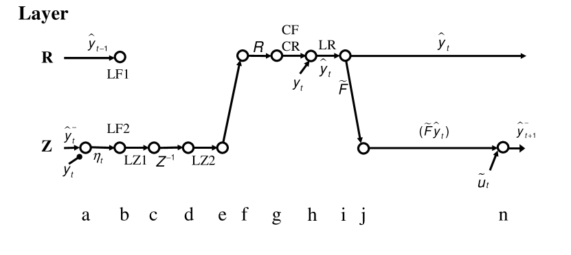
Figure 1: Layered organization of signal flow (a two-layer recurrent NN) implied by the NN algorithm for Kalman estimation (filtering and prediction) and system identification. All unfilled circles within a single layer denote the same set of $D_{\rm y}$ nodes in that layer, at each of many microsteps (time ‘ticks’) denoted a, b, $\ldots$, n. Computation proceeds from left to right along the links, for a single value of the time index $t$. At extreme right, $t$ is incremented, and signal flow resumes at extreme left. Where two inputs enter an unfilled circle, the input activity vectors are combined; arrowhead inputs are added and filled-circuit inputs are subtracted. Links labeled by a matrix denote that the activity vector at that link is multiplied by that matrix of connection strengths. Link labels starting with C and L denote where signal flow is cut (‘C’), and where signals are used for matrix learning (‘L’), during specific modes of operation (see text).

In this paper we assume that, for a hardware NN implementation, the necessary apparatus is provided to control the signal flows in the various modes, but we do not discuss such apparatus explicitly. The same is true of the apparatus for sequencing the ‘ticks.’

3.5.1 ‘Kalman mode’ of operation

We first trace the signal flows for the computation of the execution Eq. 12 using Fig. 1, which depicts the ticks within time step $t$ from left to right. The computation of Eq. 12 is part of ‘Kalman mode’ operation, defined above. We will later discuss the learning and initialization during this mode. Each (unfilled) circle denotes the set of $D_{\rm y}$ nodes in its layer, and each operation on this set of nodes is a matrix addition or subtraction of two input vectors to that circle, or a matrix multiplication of an input vector by the indicated weight matrix. At the left edge (during tick a), the new measurement input $y_{t}$ and the prediction $\hat{y}^{-}_{t}$ (which was made at the end of the previous time step) are combined in layer Z to form $\eta_{t}=\hat{y}^{-}_{t}-y_{t}$ (Eq. 11). The activity vector of the layer-Z nodes remains equal to $\eta_{t}$ until tick c. Then the lateral connections between pairs of nodes in layer Z (which include self-connections) are enabled, and the resulting activity vector at tick d is $Z^{-1}\eta_{t}$ (as discussed in the next paragraph). This activity vector is transported to layer R (between ticks e and f). The lateral connections in layer R multiply this activity vector by the matrix $R$, yielding $RZ^{-1}\eta_{t}$ at tick g. The measurement vector $y_{t}$ is added at tick h to yield $\hat{y}_{t}=y_{t}+RZ^{-1}\eta_{t}$ (Eq. 10). This vector is multiplied, between ticks i and j, by the connection strength matrix $\tilde{F}$ of feedback connections from layer R to layer Z. A control input vector $\tilde{u}_{t}$ is optionally added at tick n (the tick letters skipped here are reserved for later use), to yield $\hat{y}^{-}_{t+1}$ (Eq. 10), which is the prediction of $Y_{t+1}$, the ‘ideal noiseless measurement’ at time $t+1$. The right edge of Fig. 1 is understood to loop back to the left edge as the time index is advanced by one step; thus the activity vectors $\hat{y}_{t}$ in layer R and $\hat{y}^{-}_{t+1}$ in layer Z at tick n are relabeled $\hat{y}_{t-1}$ and $\hat{y}^{-}_{t}$, respectively, at tick a of the next time step.

How are $\tilde{Z}$ or $Z^{-1}$ learned, and $\tilde{F}$ refined, during Kalman mode? If the lateral connections in layer Z are to embody the weight matrix $\tilde{Z}$ (Method 1 of section 3.3) then Hebbian learning at link LZ1 (between ticks b and c) implements Eq. 16 using the activity vector $\eta_{t}$. The iterative computation of Method 1 then produces the output $Z^{-1}\eta$ for each $\eta$, using the connections $\tilde{Z}$. Alternatively, if the lateral connections are to embody $Z^{-1}$ (Method 2), then Hebbian learning at link LZ2 implements Eq. 17, using $(Z^{-1})_{t}\eta_{t}$, which is the activity vector at tick d after one pass of $\eta_{t}$ through the $Z^{-1}$ connections. Finally, $\tilde{F}$ updating is performed by Hebbian learning across the $\tilde{F}$ connections between layers R and Z at tick b (indicated by the labels LF1 and LF2 in Fig. 1). The activities at the two sets of nodes at tick b are $\hat{y}_{t-1}$ and $\eta_{t}$, yielding Eq. 20. (That is, the $\tilde{F}$ connections are used at tick b for updating $\tilde{F}$. Since these connections are being used to multiply an activity vector by $\tilde{F}$ only between ticks i and j, but not at tick b, no line is drawn between the layers at tick b in Fig. 1.)

At the beginning of ‘Kalman mode,’ $\tilde{Z}\equiv I-cZ$ is initialized by taking $Z$ to be an arbitrary positive-definite symmetric matrix. If $N_{\rm feat}$ is sufficiently large, it can be convenient (and in keeping with the initialization given below Eq. 12 and used in Appendix A) to choose $Z_{0}=\langle\eta_{0}\eta^{\prime}_{0}\rangle_{p}$. This choice is not required in practice, however.

3.5.2 ‘Offline sensor’ mode for learning $R$

In this mode we cut off signal flow at the line labeled CR (‘C’ denotes ‘cutoff’) in layer R between ticks g and h, and we also cut off input from the external plant, so that the sensors are running ‘offline’ and they provide only measurement (sensor) noise to the network at the input labeled $y_{t}$ at tick h; i.e., $y_{t}=n_{t}$ in Eq. 2. Then the activity vector in layer R at the line labeled LR (‘L’ denotes ‘learning’) between ticks h and i is just $n_{t}$, and Hebbian learning (at link LR) of the lateral connection strengths within layer R yields $R\approx E(n_{t}n^{\prime}_{t})$. No further processing is done during this mode of operation. (When $\gamma_{R}<1$ in Eq. 19, it is convenient to initialize $R$ to the zero matrix.)

3.5.3 ‘Initial $\tilde{F}$ learning’ mode

In this mode, we cut off signal flow at the line in layer R labeled CF, between ticks g and h. Then the activity vector in layer R is $y_{t}$ (rather than $\hat{y}_{t}$) after tick h of the current time step, and remains so until tick b of the next time step, where it is called $y_{t-1}$ since $t$ has been incremented by one. In layer Z, the activity after tick n is $\tilde{u}_{t}+\tilde{F}y_{t}$, so the activity at tick b of the next time step is $\tilde{u}_{t-1}+\tilde{F}_{t-1}y_{t-1}-y_{t}=\epsilon_{t}$ (defined just before Eq. 7). Thus the Hebbian learning rule at step b uses the activity vectors that are on line LF1 (layer R) and line LF2 (layer Z) to update the connection matrix $\tilde{F}$ between those layers, and the rule is as given by Eq. 18.

$\tilde{F}$ may be initialized to be an arbitrary $D_{\rm y}\times D_{\rm y}$ matrix.

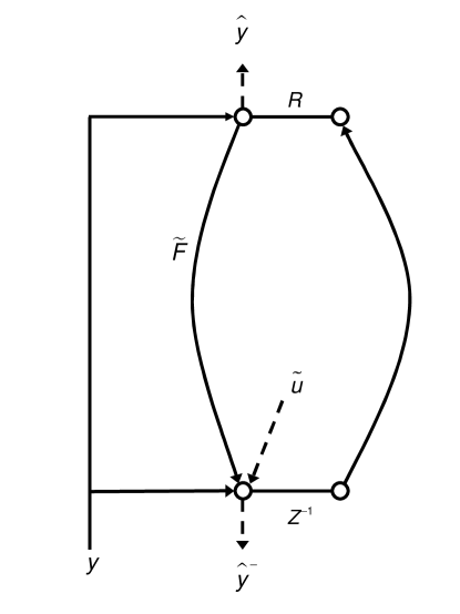
Figure 2: The NN circuit required to enable the signal flow of Fig. 1. Within each layer, the pair of circles denotes the set of $D_{\rm y}$ nodes, and the labeled line joining them denotes the weight matrix (or its inverse) of the lateral connections in that layer. Dashed lines denote optional input or output connections. Additive and subtractive inputs are not distinguished here; both are indicated by arrowheads.

3.5.4 Circuit diagram

The static neural circuit for Kalman estimation and system identification – showing all connections, but omitting the explicit time flows – is shown in Fig. 2. The signal flows detailed in Fig. 1 can easily be traced through this circuit. Optional input $\tilde{u}$ and optional outputs $\hat{y}$ and $\hat{y}^{-}$ are indicated by dashed lines. (Figures 1 and 2 are, apart from minor modifications, subsets of Figs. 4 and 5, which depict the neural circuit diagram for the fully integrated algorithm, comprising Kalman control as well as estimation and system identification. For a discussion of the relation between the signal flows and the static circuit for the full algorithm, as well as a summary block diagram of the full algorithm, see section 5.1 and Appendix B.)

3.6 Numerical example

Numerical simulations (Fig. 3) illustrate that the results of the NN estimation (KF) algorithm agree with the classical KF matrix solution, apart from fluctuations that decrease (not shown) as one increases the sample size used to estimate the covariance of $\eta$ at each time step. By contrast, recall that the classical Kalman algorithm is given the exact plant state covariance $Q$ and uses matrix-times-matrix operations, not available to the NN, to compute the covariance of the estimation error.

For our example, we consider a two-dimensional plant state. The plant and measurement processes are defined by the following parameters (see section 2 for definitions): $F$ and $H$ are 2-d counterclockwise rotations about the coordinate origin by $15^{o}$ and $50^{o}$ respectively, and the plant and noise covariance matrices are $Q=10^{-5}I$ and $R=10^{-4}I$ respectively, where $I$ is the $2\times 2$ identity matrix. We take $\tilde{u}_{t}\equiv 0$.

The learning rates are preferably allowed to be time-varying for more efficient learning. Here, the learning rates $\tilde{\gamma}_{Z}\equiv\gamma_{Z}/N_{\rm feat}$ and (in run 4 below) $\tilde{\gamma}_{F}\equiv\gamma_{F}/N_{\rm feat}$ are adaptively adjusted using the method of Murata et al. (1997). In their notation, the values of the rate control parameters, which we have made no attempt to optimize, are $\{\alpha,\beta,\gamma,\delta\}=\{0.5,30,0.05,0.1\}$ for $Z$, and $\{0.1,3,0.05,0.04\}$ for $\tilde{F}$.

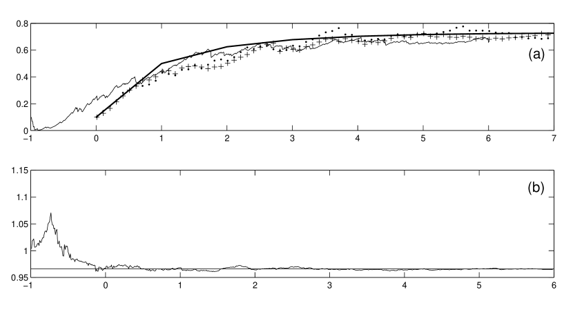
Figure 3: (a) Example of classical and neural Kalman filter learning. The (2,2) component of the $2\times 2$ matrix $(I-HK_{t})=RZ_{t}^{-1}$ (see text just before Eq. 9) is plotted vs. time step $t$, for each of four computational methods. See text (section 3.6) for details. (b) Learning of (2,2) component of $\tilde{F}$ vs. $t$, starting with arbitrary matrix. Horizontal line denotes true value of $\tilde{F}_{22}$.

In Figure 3a, the (2,2) component of the $2\times 2$ matrix $(I-HK_{t})=RZ_{t}^{-1}$ is plotted vs. time step $t$, for four different runs. All runs start with the same arbitrary $(I-HK_{0})$. The learning of the measurement noise covariance matrix $R$ is not shown here; $R$ is assumed already known.

Run 1 (thick solid curve): The classical Kalman Eqs. 4 are run for 7 time steps, and the resulting values are connected by straight line segments. Note that the results are identical when the transformed matrix Eq. 9 is used in place of Eqs. 4.

Run 2 (dotted curve): The neural network KF algorithm derived in this paper is used. In this run, one feature (a measurement vector $y$) is tracked for 700 time steps; i.e., $N_{\rm feat}=1$. Here the displayed time scale is compressed 100-fold. Every tenth value is plotted for better readability.

Run 3 (curve denoted by ‘+’ signs): The same NN algorithm, but tracking $N_{\rm feat}=100$ independent and simultaneously tracked features for 7 time steps. [Here, we update $Z$ incrementally for each feature $p=1,\ldots,N_{\rm feat}$, rather than batch-averaging all $p$, at a given time step. Thus $N_{\rm feat}$ values of $(I-HK)$ are computed during each unit time interval.] Every tenth value is plotted.

Runs 1-3 are all computed using the true fixed value of $\tilde{F}$.

Run 4 (thin solid curve): Same as for run 3, but here $\tilde{F}$ is initially arbitrary and is learned from the measurement stream. In the plot of this run, the time values are left-shifted by one unit relative to the curves for runs 1-3, in order to compensate for the startup time required to learn $\tilde{F}$ approximately. Referring to the values $t_{\rm plot}\equiv t-1$ on the abscissa of this time-shifted plot: We update $\tilde{F}$ using the raw measurement values $y$ from $t_{\rm plot}=-1$ to $0$, because $Z$ is initially arbitrary and cannot yet give useful estimates. For $t_{\rm plot}>0$, we update $\tilde{F}$ using the estimates $\hat{y}$ that depend on $Z$. We start updating $Z$ at $t_{\rm plot}=-1$, even though this update uses values of $\tilde{F}$ that are initially arbitrary and not yet reliably learned. (For additional technical detail regarding runs 3 and 4, see the last paragraph of this section.)

The learned value of the (2,2) component of $\tilde{F}$, from run 4, is plotted vs. $t_{\rm plot}$ in Fig. 3b. Note that the observations used to learn $\tilde{F}$ must span a sufficient portion of the dynamical space for learning to be adequate. For example, if the measurement vectors $y$ used to learn $\tilde{F}$ were to have values that span a significant range only in their first component, then the (1,1) component of $\tilde{F}$ would be well learned, but the (2,2) component would not. By way of contrast, as noted in section 2, classical Kalman estimation assumes that the true $F$ and $H$ have been specified to the algorithm.

Additional technical details regarding runs 3 and 4: Run 4 is generated by defining, at the starting time $t=0$ and for $1\leq p\leq N_{\rm feat}$: $\tilde{F}_{0}(p)\equiv\tilde{F}_{0}$, $Z_{0}(p)\equiv Z_{0}$, and $\hat{y}_{0}(p)\equiv y_{0}(p)$, where $\tilde{F}_{0}$ and $Z_{0}$ are arbitrary matrices and $y_{0}(p)$ is the measurement vector of the $p$th feature at $t=0$. The matrices are then incrementally learned as follows:

For $t=1,2,\ldots$:

For $p=1,2,\ldots,N_{\rm feat}$, calculate:

$$\eta_{t}(p) = \tilde{F}_{t}(p-1)\hat{y}_{t-1}(p)-y_{t}(p)~{}~{};$$

$$\tilde{F}_{t}(p) = \tilde{F}_{t}(p-1)-\tilde{\gamma}_{F}\eta_{t}(p)y^{\prime}_{t-1}(p)~{}~{};$$

$$Z_{t}(p) = (1-\tilde{\gamma}_{Z})Z_{t}(p-1)+\tilde{\gamma}_{Z}\eta_{t}(p)\eta_{t}(p)~{}~{}.$$ (21)

(Run 3 is generated in the same way as run 4, except without $\tilde{F}$ learning.) Here $\tilde{F}_{t}(p-1)$ is understood to mean $\tilde{F}_{t-1}(N_{\rm feat})$ when $p=1$, and similarly for $Z$, $\hat{y}$, and $y$. These three equations correspond, respectively, to: Eqs. 10 and 11; Eq. 18 when $t=1$ or Eq. 20 when $t>1$; and Eq. 15. That is, at each $t$, the algorithm cycles through the features one at a time, updates $\tilde{F}$ and $Z$, then uses the most recent values of $\tilde{F}$ and $Z$ to perform the update for the next feature. The first of Eqs. 21 differs subtly from Eqs. 10 and 11, since it uses $\tilde{F}_{t}(p-1)\hat{y}_{t-1}(p)$ for more efficient computation, rather than $\tilde{F}_{t-1}\hat{y}_{t-1}(p)$.

4 Neural algorithm for optimal Kalman control

As we did above for Kalman estimation, we first transform the classical Kalman control equations, then show how to implement them in an NN. The NN algorithm and signal flows for Kalman control are integrated into those derived above for Kalman estimation and system identification.

To pass from Eqs. 6 to new equations in measurement space, we define the transformations:

$$\tilde{g}\equiv H^{\prime+}B^{\prime+}gB^{+}H^{+}~{}~{}; ~{}~{}\tilde{r}\equiv H^{\prime+}rH^{+}~{}~{};$$

$$\tilde{L}_{\tau}\equiv-HBL_{\tau}H^{+}~{}~{}; ~{}~{}T_{\tau}\equiv H^{\prime+}S_{\tau}H^{+}+\tilde{g}~{}~{}.$$ (22)

The transformed matrix equation that corresponds exactly to Eqs. 6 is then

$$T_{\tau-1}=\tilde{F}^{\prime}\tilde{g}(I-T_{\tau}^{-1}\tilde{g})\tilde{F}+\tilde{r}+\tilde{g}$$ (23)

(see Appendix A.2 for proof). Similarly to the case of NN Kalman estimation, we will represent $T_{\tau}$ as the covariance of the distribution of a stochastic activity vector $w_{\tau}$, so that the learning rule for $T_{\tau}$ may be recast as an evolution equation for $w_{\tau}$. However, whereas the physically meaningful quantity $\eta_{t}$ was the vector whose covariance equaled $Z_{t}$ in the case of estimation, we now have to construct $w_{\tau}$ from terms that are based on the goal of the control problem, i.e., the cost function to be minimized.

We introduce the activity vector $w_{\tau}$, and construct a rule for computing $w_{\tau-1}$ in terms of $w_{\tau}$, such that $E(w_{\tau}w^{\prime}_{\tau})$ satisfies the same evolution equation as $T_{\tau}$ (Eq. 23):

$$w_{\tau-1}=-\nu^{g}_{\tau-1}+\nu^{r}_{\tau}+\tilde{F}^{\prime}(\nu^{g}_{\tau}+\tilde{g}T_{\tau}^{-1}w_{\tau})$$ (24)

(see Appendix A.2 for proof). Here $\nu^{g}_{\tau}$ and $\nu^{r}_{\tau}$ are random vectors, or internally generated ‘noise,’ drawn from distributions having mean zero and covariances $\tilde{g}$ and $\tilde{r}$ respectively. These noise generators are the means by which the neural network represents the cost matrices $\tilde{g}$ and $\tilde{r}$. Note that we have a learning rule for $T_{\tau}$, but need to compute $(T^{-1})_{\tau}w_{\tau}$ in Eq. 24; thus $T$ here plays the role analogous to $Z$ in neural Kalman estimation, and the present computation is handled using the same methods (see next paragraph).

Learning: At the current time $t_{0}$, a set of KC matrices $T_{\tau}$ to be used at future times is learned by iteratively computing Eq. 24 for $\tau=N,N-1,\ldots,t_{0}+1$, starting with $w_{N}=\nu^{r}_{N+1}-\nu^{g}_{N}$ (corresponding to $S_{N}=r$). In the idealized limit in which the sample average converges to the expectation value for the $w_{\tau-1}$ distribution – i.e., $\langle w_{\tau-1}w^{\prime}_{\tau-1}\rangle\rightarrow E(w_{\tau-1}w^{\prime}_{\tau-1})$ – neural control learning using $T_{\tau-1}=\langle w_{\tau-1}w^{\prime}_{\tau-1}\rangle$ exactly yields optimal Kalman control. In practice, we use either Method 1 of section 3.3 above, using the update rule for $(I-cT)$ (cf. Eq. 15) where $T_{\tau-1}=(1-\gamma_{T})T_{\tau}+\gamma_{T}\langle w_{\tau}w^{\prime}_{\tau}\rangle_{p}$; or Method 2 (cf. Eq. 17), using $(T^{-1})_{\tau-1}=(1+\gamma_{T})(T^{-1})_{\tau}-\gamma_{T}\langle w_{\tau}w^{\prime}_{\tau}\rangle_{p}$ with the same caveats that were described for $Z^{-1}$ in section 3.3. Either method yields an approximation to the optimal Kalman controller that is limited in accuracy only by the deviations between sample averages and expectation values. (Unlike the case of Kalman estimation, in which $N_{\rm feat}$ is limited by the number of available features to be tracked, here the $w_{\tau}$ values are internally computed, so one can in principle use arbitrarily many independent $w_{\tau}(p)$ values at each value of the time index $\tau$.)

Execution: For any or all of the time steps $t=t_{0},\ldots,N$, the $T_{t}$ or $(T^{-1})_{t}$ computed above can now be used to compute the desired control signal

$$\tilde{u}_{t}=\tilde{L}_{t}\hat{y}_{t}=(-I+T_{t}^{-1}\tilde{g})\tilde{F}\hat{y}_{t}~{}.$$ (25)

For a software implementation, it is most convenient to store the sequence of $T$ or $T^{-1}$ matrices during learning, and retrieve them in reverse order during execution. In hardware, one can choose either to (a) store and retrieve as above (possibly using different parts of a larger NN to store each matrix, not discussed here), or (b) retain only the last-computed matrix $T_{t_{0}}$, use it for execution at the current time $t_{0}$, then relearn the $T$ matrices at the next time step $t_{0}+1$. Alternatively, one may (c) approximate ideal KC by using the same computed matrix for several time steps.

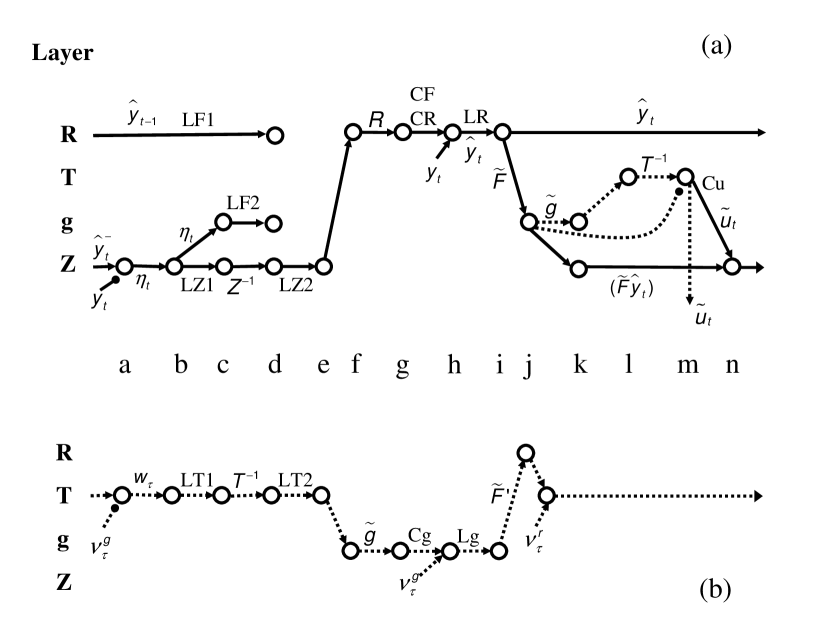
Figure 4: Layered organization of signal flow required by full NN algorithm for Kalman estimation, system identification, and Kalman control. (a) Signal flow for system identification and for learning and execution of Kalman estimation (solid links), and for execution of Kalman control (dashed links), shown in a four-layer recurrent NN, all at time $t$. Other notation as in Fig. 1. (b) Signal flow for learning of Kalman control (dashed links), shown separately in the same four-layer NN, all at time index $\tau$ of the KC learning process. At extreme right, $\tau$ is decremented, and signal flow resumes at extreme left. Other notation as in Fig. 1.

To show how the learning and execution of Kalman control (KC) is added to the neural network, we refer to Figs. 4 and 5. Figure 4a (for KC execution) is essentially Fig. 1 augmented by two additional layers, denoted T and g (the latter label not to be confused with ‘tick g’ on the horizontal axis), and with additional processing (indicated by the dotted lines between ticks j and n) to compute $\tilde{u}_{t}$ using the new weight matrices $T$ (or $T^{-1}$) and $\tilde{g}$. The learning of these matrices is performed by the processing described in Fig. 4b, which takes place during different modes of operation (to be described) than does the processing described by Fig. 4a. Since KC learning involves some special features not encountered in KF learning, we first consider Fig. 4a, which embodies KF learning and execution, combined with KC execution (but not KC learning).

The new processing begins in layer g at tick j. Note that the $\tilde{F}$ connections now go from layer R to g (rather than to Z as in Fig. 1). The activity vector at layer g and tick j is thus $\tilde{F}\hat{y}_{t}$, and this activity is passed on unchanged to layer Z at tick k. From tick j to tick m, the activity vector computed by the two dotted-line signal flows is $\tilde{u}_{t}=(T^{-1}\tilde{g}-I)\tilde{F}\hat{y}_{t}$ (as required by Eq. 25). Since $\tilde{g}$ and $T$ (or $T^{-1}$) are the weights on two different sets of lateral connections, we have assigned each of these connection matrices to a different layer (g and T respectively). The vector $\tilde{u}_{t}$ is provided as output from the network to effector ‘organs’ (which act on the external plant), and is also provided as an ‘efferent copy’ to the network itself (at tick n), where it is used to compute the prediction $\hat{y}^{-}_{t+1}$.

Unlike the case of KF, where $Z$ or $Z^{-1}$ is learned as part of the same process that computes the predictions $\hat{y}^{-}$, here the KC learning process (updating of $T$ or $T^{-1}$, and of $g$) must be done separately from KC execution (computation of $\tilde{u}$). The same four layers are used for both KC learning and execution, but at different times and in different modes. Thus, at a particular value of the execution time index $t=t_{0}$, the network processing mode is changed from ‘Kalman mode’ (which now includes KC execution) to ‘KC learning mode,’ in which a sequence of steps for the KC learning time index $\tau=N,N-1,\ldots,t_{0}+1$ is performed. See Appendix B for further discussion.

The KC learning process is described in Fig. 4b. The time step is labeled $\tau$, and this label is decremented by one when we pass from tick n to tick a. The shift in mode from Kalman mode to KC learning mode can either be made at each time step $t$ [as in implementation (b) following Eq. 25], or at only some time steps $t$ if means are provided to store the computed values of $T$ or $T^{-1}$ [as in implementations (a) and (c) above].

Learning of $\tilde{g}$ is analogous to that of $R$: The signal flow is cut off at link Cg (before tick h), so that the only input to the layer-g nodes at tick h is the structured noise term $\nu^{g}_{\tau}$. Then Hebbian learning at the lateral layer-g connections implements $\tilde{g}\approx E[\nu^{g}_{\tau}(\nu^{g}_{\tau})^{\prime}]$. No further processing occurs during this mode.

For $T$ (or $T^{-1}$) learning, the entire signal flow pathway of Fig. 4b is active. Starting at tick a, the activity vector $w_{\tau}$ yields the following activity vectors at subsequent ticks:

1. $T^{-1}w_{\tau}$ at tick d;

2. $\tilde{g}T^{-1}w_{\tau}$ at tick g;

3. $\nu^{g}_{t}+\tilde{g}T^{-1}w_{\tau}$ at tick h;

4. $\nu^{r}_{\tau}+\tilde{F}^{\prime}(\nu^{g}_{t}+\tilde{g}T^{-1}w_{\tau})$ at tick k;

5. $w_{\tau-1}=-\nu^{g}_{\tau-1}+\nu^{r}_{\tau}+\tilde{F}^{\prime}(\nu^{g}_{t}+\tilde{g}T^{-1}w_{\tau})$ at tick a of the new time step $\tau-1$.

The last equality comes from Eq. 24.

The activity vector $w_{\tau}$ is used to update $T$ or $T^{-1}$ in the same way that $\eta_{t}$ was used to update $Z$ (Method 1) or $Z^{-1}$ (Method 2) in the Kalman estimation algorithm (section 3.3). Thus, using Method 1, Hebbian learning at link LT1 implements $T_{\tau}\approx E(w_{\tau}w^{\prime}_{\tau})$. Alternatively, using Method 2, Hebbian learning at link LT2 implements

$$(T^{-1})_{\tau-1}=(1+\gamma_{T})(T^{-1})_{\tau}-\gamma_{T}\langle[(T^{-1})_{\tau}w_{\tau}][(T^{-1})_{\tau}w_{\tau}]^{\prime}\rangle_{p}$$ (26)

(subject to the same requirements on $\gamma_{T}$ and $T^{-1}$ symmetry that were discussed in section 3.3 for the case of $Z^{-1}$ learning). The learning is Hebbian, since the activity at tick d after one pass of $w_{\tau}$ through the $T^{-1}$ connections is $[(T^{-1})_{\tau}w_{\tau}]$.

Note that the $\tilde{F}^{\prime}$ connections in Fig. 4b are shown as a signal flow line passing from layer g to R followed by a line from R to T, rather than passing directly from layer g to T. This distinction is irrelevant to a software implementation, but is shown here because $\tilde{F}^{\prime}$ is learned using a Hebbian rule that is identical to that used for $\tilde{F}$, and consequently it is convenient for $\tilde{F}$ and $\tilde{F}^{\prime}$ to connect the same two layers (g and R), in opposite directions, in a hardware implementation. $\tilde{F}$ and its transpose $\tilde{F}^{\prime}$ may be thought of as the same physical set of symmetric connections in an artificial hardware implementation that allows bidirectional connections. In a model that permits only unidirectional connections (in both directions), e.g., a model of a biological network, $\tilde{F}$ and $\tilde{F}^{\prime}$ would be thought of as distinct sets of connections. Even in the latter case – since the same Hebbian rule is applied to both, with the same pair of activities at the two ends of each pair of connections – the two sets will nonetheless learn matrices that are the transpose of each other, apart from differences resulting from initialization, processing noise, and possibly faulty or missing connections.

5 Discussion

We have shown how to perform the learning and execution of Kalman estimation and control, as well as system identification, using a neural network. The method is asymptotically exact in the limit that certain sample averages of computed quantities approach the corresponding expectation values over the distributions of those quantities. The matrices $Z$ and $T$ that are iteratively computed, in order to learn and execute KF and KC respectively, are each equal to the covariance of a distribution of computed activity vectors. In each case, vectors evolve over time via a sequence of transformations performed by the NN, and are used, via Hebbian learning, to update a matrix of connection weights that represents the KF or the KC matrix. The logical path of the derivation proceeds from the classical Kalman solutions, to a transformed set of equations that involves only quantities measured by the NN, to a set of signal flows and computations, and finally to a layered NN architecture and circuitry that supports those computations.

Both the signal flows and the NN architecture appear to be constrained by the requirements of the Kalman neural algorithm (apart from small variations); that is, they do not appear to represent merely one among a large number of disparate possible choices of architecture or signal flow.

In the remainder of this section, we discuss

1. the considerations that constrain the architecture and signal flows;

2. applications to artificial NN design, and prior work; and

3. resemblances between the derived architecture and biological networks in neocortex, and caveats involved in drawing inferences regarding biological function.

5.1 Constraints on NN architecture and signal flows implied by the neural Kalman algorithm

The assignment of activity vectors to distinct NN layers, and details of the signal flow among layers, are significantly constrained by several requirements:

1. Each of the four matrices $R$, $\tilde{g}$, $Z$ (or $Z^{-1}$), and $T$ (or $T^{-1}$), is learned using a Hebb rule that contains a product of the form $vv^{\prime}$; i.e., in each case the activity vectors at the source and target ends of the connection matrix are the same. (See Eq. 14 with $z\equiv v$ for $R$ and $\tilde{g}$ learning; Eq. 16 or 17 for $Z$ or $Z^{-1}$ learning; and the corresponding equations for $T$ or $T^{-1}$ learning.) When the Hebb rule is of this form, it is natural to implement the connection matrix as joining each node (of the set of $D_{\rm y}$ nodes) to each node (including itself) of the same set of nodes. Thus each such matrix describes a set of lateral connections, and is assigned to its own layer, denoted by R, g, Z, T in each of Figs. 4a and 4b.

2. For Hebbian learning, activity $\eta_{t}$ must be present at the input to the $Z$ (or $Z^{-1}$) connections; $w_{\tau}$ at the input to $T$ (or $T^{-1}$); $y_{t}\equiv n_{t}$ at the input to $R$ during $R$ learning mode; and $\nu^{g}_{\tau}$ at the input to $\tilde{g}$ during $\tilde{g}$ learning mode.

3. For Hebbian learning of $\tilde{F}$, activities $\hat{y}_{t-1}$ and $\eta_{t}$ must be present simultaneously at the two ends of the $\tilde{F}$ matrix. Thus $\hat{y}_{t-1}$ must be held as the activity of one set of nodes in layer R (of Fig. 1 or 4a) until $\eta_{t}$ has been computed at layer Z and made available at layer Z (of Fig. 1) or layer g (of Fig. 4a). $\tilde{F}$ is updated at the time indicated by links LF1 and LF2, but is used later in the signal flow, at the link labeled $\tilde{F}$.

4. The transpose matrix $\tilde{F}^{\prime}$ is required for KC learning (Fig. 4b). $\tilde{F}^{\prime}$ is learned by the same algorithm, and at the same time, as $\tilde{F}$; thus it is assigned to connect the same two layers as $\tilde{F}$, but in the reverse direction. Figure 4 assigns $\tilde{F}$ to run from layer R to g, and $\tilde{F}^{\prime}$ from g to R; this requires $\eta$ to be copied from layer Z to g as shown (just before LF2). [As a slight variant, $\tilde{F}$ could run instead from R to Z; then $\eta$ would not need to be copied from Z to g, but the solid path (Fig. 4a) would require a Z $\rightarrow$ g link just following the $\tilde{F}$ link from R to Z for KC execution, and the dashed path (Fig. 4b) would require a g $\rightarrow$ Z link following link Lg, to connect to $\tilde{F}^{\prime}$.]

5. The measurement vector $y_{t}$ is required twice as input: to layer Z, where it contributes to $\eta_{t}$, and to layer R, where it combines with $RZ^{-1}\eta_{t}$ to yield $\hat{y}_{t}$.

Thus the arrangement shown in Fig. 4 is not an arbitrary way of laying out the NN algorithms we have derived; rather, the four-layer organization and its signal flows appear to be substantially determined (apart from small variations) by the algorithms and the requirements of a NN implementation.

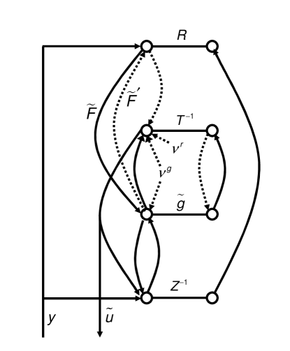
Figure 5: NN circuitry required to enable the signal flow of Fig. 4. Within each layer, the pair of circles denotes the set of $D_{\rm y}$ nodes, and the labeled line joining them denotes the weight matrix (or its inverse) of its lateral connections. Dashed lines denote connections that are only involved in KC learning. Other notation as in Fig. 2.

The static neural circuit for the integration of Kalman estimation and control, as well as system identification – showing all connections, but omitting the explicit time flows – is shown in Fig. 5. The signal flows of Fig. 4 can be traced through this circuit (see Appendix B.1 as an aid). The circuit operation comprises several modes (requiring appropriate functional switching) including: (a) learning of the $\tilde{F}$ and $\tilde{F}^{\prime}$ connection weight matrices (system identification); (b) normal ‘online’ KF and execution of KC (‘Kalman mode’); (c) iterative learning of the KC matrices $T$; and (d) initial or intermittent learning of matrices $R$ (for KF) and $\tilde{g}$ (for KC). Optional outputs $\hat{y}$, $\tilde{F}\hat{y}$, $\hat{y}^{-}$, and/or $\eta$ can be provided (not shown) from layers R, g (or Z), Z, and Z (or g) respectively.

5.2 Engineering applications and prior work

As a mathematical and engineering method, these NN algorithms may prove useful for implementing estimation, control, and system identification in special-purpose hardware comprising simple computational elements, especially with a large number of sets of such elements operating in parallel. Even when the plant or measurement parameters change with time, the present NN algorithms learn the new dynamics automatically and converge to the new optimal solution after a transient period of adjustment. The well-known extended Kalman filter (EKF) (Haykin, 2001) and its variants yield approximate solutions for nonlinear plant and measurement processes, by repeatedly linearizing the dynamics about an operating point. Our NN algorithms likewise yield approximate solutions in these cases, since the learned plant and measurement parameters are automatically updated in response to the changing stream of noisy measurements (see text just below Eq. 8).

In earlier work, neural networks have been used in conjunction with the Kalman filter (KF) or Kalman control (KC) equations in several ways:

The classical KF or EKF (extended Kalman filter) equations have been used to compute how the weights in a NN should be modified. The NN weights to be determined are treated as the unknown parameter values in a system identification problem, sets of input values and desired output values are specified, and the KF or EKF equations are used to determine the NN weights based on the sets of input and desired-output values. The equations are solved by means of conventional mathematical steps including matrix multiplication and inversion. That is, the weights are not computed or updated by means of a neural network. Instead, the weights are read out from the neural network, provided as input arguments to the KF or EKF algorithm (which is not a NN algorithm), the updated weight values are then provided as outputs of the KF or EKF algorithm, and the updated weight values are then entered into the neural network as the new weight values for the next step of the computation. For examples of this combined usage of a NN in conjunction with the classical KF or EKF equations, see (Haykin 2001, Rivals & Personnaz 1998, Singhal & Wu 1989, Williams 1992). Rao & Ballard (1997) also describe an EKF algorithm for weight update, but do not address how the algorithm (with its matrix-times-matrix computations and matrix inversion) could be implemented in a NN whose units have limited computational power.

The output from a nonlinear NN has been used in conjunction with that of a classical (non-neural) KF algorithm, to improve predictions when applied to a nonlinear plant process (Klimasauskas & Guiver 2001, Tresp 2001).

A NN algorithm for KC (Szita & Lőrincz, 2004), using temporal-difference learning, performs KC in the special case of stationary control, but is not applicable to the general KC case. In the stationary control problem there is no specified time-to-target $N$; instead, the time remaining to the goal is either infinite, or is selected at each succeeding time step from a distribution that does not change with time.

A recent KF-inspired NN algorithm (Szirtes, Póczos, & Lőrincz, 2005) is described as a ‘neural Kalman filter.’ However, it substantially alters Kalman’s formulation, to the extent that the resulting NN does not in general implement KF, even approximately. Although the initial prediction error (starting with an arbitrary prediction) is shown to decrease rapidly with time, this provides no evidence that the KF has been even approximately learned. Indeed, a similar reduction in error is found even when an arbitrary, non-optimal, and unchanging filter, differing greatly from the true KF, is used. See Appendix C for details.

5.3 Comparison with biology – background

Mammalian neocortex exhibits a significant degree of uniformity in its layered architecture and pattern of interlaminar connectivity, although there are also well-known variations among cortical areas (Mountcastle, 1998). A focus on the properties that are similar across cortical areas and species has led to models of neocortex that have, as a basic unit on the 50- to 100-micron scale, the so-called local cortical circuit (LCC, minicolumn, canonical microcircuit) (Callaway, 1998; Douglas & Martin, 2004; Gilbert, 1983; Mountcastle, 1998). The observed uniformity also motivates a search for a set of core LCC processing functions that may be common to sensory, motor, and other cortical areas, and that may enable the diverse functions of those areas (Grossberg & Williamson, 2001; Poggio & Bizzi, 2004).

The blending of ‘bottom-up’ sensory input and ‘top-down’ model-driven expectations has been discussed in the context of Bayesian inference and generative models, and various neural network (NN) algorithms are motivated by, approximate, or perform a portion of, the Bayesian inference process (e.g., George & Hawkins, 2005; Hinton & Ghahramani, 1997; Hinton, Osindero, & Teh, 2006; Lee & Mumford, 2003; Lewicki & Sejnowski, 1997; Rao, 1999; Rao, 2004; Rao, 2005; Todorov, 2005; Yu & Dayan, 2005; Zemel et al., 2005). The use of bottom-up and top-down signals in these algorithms has been noted to be reminiscent of the feedforward and feedback connections, both between different cortical areas and within the LCC. Bayes-optimal behavior has been found in human psychophysics experiments (e.g., Körding & Wolpert, 2004). Kalman filtering is well known to be, under certain conditions, an exactly solvable special (linear) case of Bayesian inference.

I consider it plausible that the core functions of the LCC include the prediction of future sensory input, the estimation of noisy or missing input, and the generation of control outputs, and that these functions are performed at multiple levels in sensory, motor, and other cortical areas. Part of the motivation for the present work has been to explore this conjecture. To do this, it has appeared fruitful to ask: Is an implementation of Kalman’s methods for optimal estimation and control possible within an artificial neural network composed of simple processing nodes? If so, what does such an implementation appear to require of the network’s architecture and processing – how the network is divided into layers, the connections between and within layers, timing considerations, etc.? The results we have presented here suggest that requiring a neural network to implement the Kalman solutions imposes significant constraints on the network’s form. Because of this, resemblances that are observed between the artificial and biological networks may have greater potential significance than they would have if the form of an artificial Kalman neural network were quite unconstrained. However, any such comparison between the artificial and biological networks involves many caveats, as we discuss next.

5.4 Comparison with biology – the neural Kalman circuit and the LCC

This subsection is necessarily speculative. Here we show, first, that our KPC NN architecture, to which we have been led by the above constraints, bears certain resemblances to the observed architecture (layered organization, and the connectivity among layers, inputs, and outputs) of the LCC. This is consistent with the conjecture that the LCC’s core functions include those of estimation (prediction and filling-in of missing or noisy data) and control, albeit in the context of nonlinear systems, interactions, and feature discovery and analysis, rather than in the simpler linear (or linearizable) Kalman context.

After identifying the resemblances, we turn to the differences between the Kalman NN and the LCC, and to caveats that limit our current ability to use the approximate Kalman-LCC ‘mapping’ to draw inferences regarding possible LCC function.

5.4.1 Resemblances

1. The KPC NN and the LCC are both recurrent neural networks. Given the iterative nature of the classical Kalman algorithms, this is an unsurprising feature of the Kalman NN.

2. The KPC NN has four layers (two if only Kalman estimation and system identification, but not control, are considered). The LCC is typically treated as having four layers (denoted as layers 6, 5, 4, and 2/3), of which three (layers 6, 4, and 2/3) are considered important for sensory (as distinct from motor control) processing.

3. The ‘sensory’ input to the KPC NN is required to enter at two layers (denoted as layers Z and R). Input to layer R (at tick h of Fig. 4a) may be regarded as primary, and that to layer Z as modulatory, in the sense that the raw measurement $y_{t}$ enters layer R as the primary contribution to the computation of the estimate $\hat{y}_{t}$, while $y_{t}$ enters layer Z (at tick a of Fig. 4a) in order to compute the Kalman correction [which is $RZ^{-1}(\hat{y}^{-}_{t}-y_{t})$] to the raw measurement. Inputs to the LCC from ‘lower’ levels of a sensory hierarchy (as usually conceived) are to layers 6 and 4, with the input to layer 4 considered as dominant, and that to layer 6 as modulatory. In the LCC, unlike our linear NN, these inputs can interact nonlinearly.

4. The Kalman estimate of the present state, $\hat{y}_{t}$, is available as output from layer R, and the Kalman control signal $\tilde{u}_{t}$ from layer T. (The prediction of the state at the next time step, $\hat{y}^{-}_{t+1}$, is also available from layer Z.) In the LCC, output to ‘higher’ hierarchical levels is from layer 2/3, and that to ‘lower’ levels is from layer 5. For the LCC, the layer 2/3 output signals the results of feature analyses (e.g., of features within a sensory ‘scene’) that have been performed within that cortical area. This is a nonlinear computation that can be considered analogous to linear Kalman estimation. This putative LCC computation, and Kalman estimation, both yield an improved knowledge of the external state, by suppressing noise and ‘filling in’ missing data, even though linear estimation is not capable of inferring, or making ‘decisions’ about, the presence or absence of particular features. The layer-5 LCC output provides motor control signals – again by a nonlinear process that has greater capability than, but can also be considered analogous to, or a more powerful version of, Kalman control.

We compare diagrammatically the interlaminar signal flow of the KPC NN with the putative principal signal flows (Gilbert, 1983) of the LCC. The signal flow for Kalman estimation (learning and execution) and Kalman control (execution only) (Fig. 4a) may be schematized, considering layers g and T as a unit, as Dgm. D1 (below, left):

$\{\;\;\;{\rm R}\;\;\;\}$

$\rightarrow$

(g,T)

$\rightarrow$

Z

$\rightarrow$ R

4

$\rightarrow$

2/3

$\rightarrow$

5

$\rightarrow$

6

$\rightarrow$ 4

$\uparrow\;\;\;\;\downarrow$

$\downarrow$

$\uparrow$

$\uparrow$

$\downarrow$

$\downarrow$

$\uparrow$

$y\;\;\;\;\hat{y}$

$\tilde{u}$

$y$

[D1]

in

${\rm out}_{S}$

${\rm out}_{M}$

in

[D2]

(The KC learning of Fig. 4b adds a g $\rightarrow$ R path.) By comparison, Gilbert’s (1983) proposal for the principal LCC signal flow among the layers 6, 5, 4, and 2/3 is shown in Dgm. D2 (above, right). More recent work is consistent with, and expands upon, this basic flow (Callaway, 1998; Douglas & Martin, 2004; Raizada & Grossberg, 2001). Layer 4 is elaborated in visual cortex and is much less prominent in motor than in sensory cortex, while layer 5 is more prominent in motor cortex (Mountcastle, 1998) and provides motor control output (both in motor and in sensory cortex, e.g., from V1 to superior colliculus) denoted here by ${\rm out}_{M}$. Layer 2/3 integrates contextual inputs from outside the classical receptive field, and provides output, denoted by ${\rm out}_{S}$, to other cortical areas that process ‘higher-level’ perceptual features.

We consider, in the next subsection, the extent to which it is reasonable to take seriously these resemblances between the KPC NN and the putative LCC signal flows. If we do take them as suggesting possible relationships between the functions of the two networks, we are led to at least a rough and tentative correspondence between (a) NN layer R, and LCC layers 4 and 2/3; (b) NN layer Z, and LCC layer 6; (c) NN layers g and T, and LCC layer 5; (d) NN inputs $y$ to layers R and Z, and LCC sensory inputs to layers 4 and 6, respectively; (e) motor outputs $\tilde{u}$ and ${\rm out}_{M}$, with an efferent copy to NN layer Z for prediction of the future plant state; (f) the optimal estimate $\hat{y}$, and ${\rm out}_{S}$; and (g) the g $\rightarrow$ R path of KC learning (Fig. 4b), and observed LCC connections from layer $5\rightarrow 2/3$ (not shown in D1 and D2).

We treat the g and T layers together since their role is limited to control, and since LCC layer 5 appears to be most prominent in motor control areas of cortex. We suggest that the Kalman NN may require one layer (R) in place of two (cf. LCC layers 4 and 2/3) because Kalman estimation does not involve the learning of higher-level features (e.g., orientation selectivity in V1), and we expect that more sophisticated (e.g., more strongly nonlinear and context-sensitive) NN prediction methods may require an additional layer as in the LCC.

Note that in our NN, $\tilde{F}$ (used for prediction) and $\tilde{F}^{\prime}$ (used for learning of control) connect the same pair of NN layers in opposite directions, and are learned together during system identification. This suggests that a biological network performing Kalman-like prediction and control might use a corresponding pair of functional mappings that are (approximately) the transpose of one another.

For an example of a mapping between the KPC NN and the LCC that is more detailed than I think is warranted in view of the caveats discussed below, the interested reader may see Appendix D.

5.4.2 Differences and caveats

We have compared one type of artificial NN – one that performs Kalman estimation and control, and system identification, without simplifications or approximations (beyond that entailed by approximating an expectation value over an ensemble by a finite-sample average) – with a putative and simplified biological LCC. In order to be able to draw confident inferences from any resemblances that emerge, it would be important to know whether the resemblances are robust across (a) several types of NN coding schemes, (b) a variety of relevant NN prediction and control methods, and (c) uncertainties regarding the biological network. These are open questions. Caveats and limitations therefore include the following:

1. Nature of the computational task to be performed: If the LCC performs estimation (including prediction) and control, it surely performs it in a more general fashion than does KPC – including the learning of higher-level features, and other nonlinear and context-dependent analyses (e.g., Bayesian inference and the use of generative models) – although the functions performed by the LCC might subsume KPC as simple special cases.

2. NN coding schemes and neuronal dynamics: Neuronal dynamics are much more complex than the NN operations allowed here. Despite this, it is commonly (and often fruitfully) assumed that reduced or simplified NN models can capture relevant dynamical features of biological neuronal networks. As an example, the node activity in a nonlinear (sigmoidal) version of the NN used here is often identified with an average neuronal firing rate; and connection weights, with synaptic efficacies. However, other types of NNs represent and process information in a variety of ways (Haykin, 1999; Hertz, Krogh, & Palmer, 1991), using, e.g., population coding, sparse coding, coding via precise spike timing (Rieke & Bialek, 1999), and the related use of synchronous or phase-locked firing or oscillations for conveying information, switching between functional modes, and/or more efficient learning. Detailed neuronal dynamics also affect the relative timing of excitatory and inhibitory effects, the occurrence of bursting vs. tonic firing modes, etc., all of which are absent from our simple NN.

   If a particular type of NN coding supports the basic operations used here – matrix-times-vector multiplication, addition of vectors, and bilinear Hebbian learning – then the derivation of the KPC algorithm and architecture can proceed as described, essentially unchanged at the level of abstraction depicted in Figs. 4 and 5 (the signal flows) and Fig. 6 (the block diagram discussed in Appendix B.2), although the particular way in which a vector is multiplied by a matrix will depend on the type of NN coding used. When the NN coding supports a quite different set of operations, however, it is an open question whether and how neural KPC may be implemented, and what the resulting architecture will be.

3. Question of uniqueness of our design: For our allowed set of NN operations, our exploration of the design constraints for performing general KPC suggests that the resulting signal flow and circuit are substantially determined (apart from small variations), but we cannot rule out the possibility of a significantly different design.

4. Experimental limitations: Knowledge of the detailed LCC connectivity is substantial, but not complete; e.g., an inhibitory cell may provide output to many layers, and the extent and importance of some of these connections are not clear. Knowledge of the LCC signal flows and their sequencing is also quite incomplete.

6 Conclusion

The approach taken here has been to (a) pose a well-defined computational task – Kalman prediction and control – that is a prototype of the more general and powerful prediction and control processes that are likely to be important in cortex; (b) select a simple typical set of allowed NN operations, rather than invoking more complex NN dynamics specially tailored to the task; (c) see whether a NN algorithm can be devised that does not compromise, change, or limit the computational task; (d) see what constraints that task imposes on the NN’s circuitry and signal flows; and (e) compare the resulting NN circuitry with that of the biological system of interest.

We have shown how optimal Kalman estimation and control, and system identification, can be learned and executed by a neural network having simple computational elements. In progressing from the classical Kalman equations to a NN algorithm, we have find that the computational task appears to impose significant constraints on the resulting NN architecture, circuitry, and signal flows.

When we compare the resulting architecture to that of recurrent neural circuits found in brain, and to LCC architecture in particular, we find certain resemblances. The LCC architecture has been suggested to perform core functions (as yet unknown) that underlie sensory and motor processing in general. It is plausible that such functions may include prediction, the estimation or inference of missing or noisy sensory data, and the goal-driven generation of control signals. Thus the resemblances found between the KPC NN architecture and that of the ‘local cortical circuit’ may not be coincidental.

However, before one can infer from such resemblances that the LCC is likely to be performing a particular set of core functions, much more evidence is required. The present work fits into a broader context of ongoing NN research by many workers, in which (a) a range of biologically realistic neural coding strategies (e.g., population or spike coding) is being studied, to see how simple neural computations can be carried out using these codes, and (b) a range of computational tasks in prediction and control (e.g., Bayesian inference) is being explored, to see how recurrent NNs may implement such tasks. From the experimental side, further elucidation of both the functional connectivity and signal flows in local cortical circuitry is of course also required. It will be interesting to see whether certain types of computational tasks are found to be associated with specific architectural features in NNs and, if so, whether such mappings have useful implications for understanding biological neural function.

Such continuing interaction between theory and experiment may not only contribute to elucidating core aspects of cortical function, but may also lead to insights into new methods for nonlinear estimation and control.

Appendix A. Mathematical details

Here we prove that:

1. Eq. 9 and Eqs. 4 are equivalent;

2. $Z_{t}=E(\eta_{t}\eta^{\prime}_{t})$ and the $\eta$ evolution Eq. 12 (applied to each $\eta_{t}$ in the ensemble over which the expectation value is defined) imply $Z_{t+1}=E(\eta_{t+1}\eta^{\prime}_{t+1})$;

3. Eq. 23 and Eqs. 6 are equivalent; and

4. $T_{t}=E(w_{t}w^{\prime}_{t})$ and the $w$ evolution Eq. 24 imply $T_{\tau-1}=E(w_{\tau-1}w^{\prime}_{\tau-1})$.

A.1 Neural Kalman estimation

(1) Eq. 4 for $K_{t}$, and the definition $Z_{t}\equiv HP^{-}_{t}H^{\prime}+R$, yield $I-HK_{t}=I-HP^{-}_{t}H^{\prime}Z^{-1}_{t}=I-(Z_{t}-R)Z^{-1}_{t}=RZ^{-1}_{t}$. Thus Eq. 4 yields

$$Z_{t+1} = HF(I-K_{t}H)P^{-}_{t}F^{\prime}H^{\prime}+HQH^{\prime}+R$$ (27)

$$= \tilde{F}(I-HK_{t})HP^{-}_{t}H^{\prime}\tilde{F}^{\prime}H^{\prime}+HQH^{\prime}+R$$

$$= \tilde{F}RZ^{-1}_{t}(Z_{t}-R)\tilde{F}^{\prime}H^{\prime}+HQH^{\prime}+R$$

$$= \tilde{F}(I-RZ^{-1}_{t})R\tilde{F}^{\prime}H^{\prime}+HQH^{\prime}+R~{},$$

which is Eq. 9.

(2) The plant and measurement equations for $x_{t+1}$ and $y_{t}$ yield

$$y_{t+1}=\tilde{F}Hx_{t}+\tilde{u}_{t}+Hm_{t}+n_{t+1}~{};$$ (28)

thus

$$\eta_{t+1} = -y_{t+1}+\tilde{F}y_{t}+\tilde{F}RZ^{-1}_{t}\eta_{t}+\tilde{u}_{t}$$ (29)

$$= -Hm_{t}-n_{t+1}+\tilde{F}n_{t}+\tilde{F}RZ^{-1}_{t}\eta_{t}~{}.$$

Since (a) the noise terms $m_{t}$, $n_{t}$, and $n_{t+1}$ are mutually independent and have zero mean; (b) $\eta_{t}$ depends on $n_{t}$ (through $y_{t}$) but not on $m_{t}$ or $n_{t+1}$; (c) $R$ and $Z$ are symmetric matrices; and (d) $E(m_{t}m^{\prime}_{t})=Q$, $E(n_{t}n^{\prime}_{t})=E(n_{t+1}n^{\prime}_{t+1})=R$, $E(\eta_{t}n^{\prime}_{t})=-E(n_{t}n^{\prime}_{t})=-R$, and $E(\eta_{t}\eta^{\prime}_{t})=Z_{t}$; we obtain

$$E(\eta_{t+1}\eta^{\prime}_{t+1}) = HE(m_{t}m^{\prime}_{t})H^{\prime}+E(n_{t+1}n^{\prime}_{t+1})+\tilde{F}E(n_{t}n^{\prime}_{t})\tilde{F}+\tilde{F}RZ^{-1}_{t}E(\eta_{t}n^{\prime}_{t})\tilde{F}^{\prime}$$ (30)

$$+\tilde{F}E(n_{t}\eta^{\prime}_{t})Z^{-1}_{t}R\tilde{F}^{\prime}+\tilde{F}RZ^{-1}_{t}E(\eta_{t}\eta^{\prime}_{t})Z^{-1}_{t}R\tilde{F}^{\prime}$$

$$= HQH^{\prime}+R+\tilde{F}R\tilde{F}^{\prime}-\tilde{F}RZ^{-1}_{t}R\tilde{F}^{\prime}$$

$$= \tilde{F}(I-RZ^{-1}_{t})R\tilde{F}^{\prime}+HQH^{\prime}+R~{},$$

which equals $Z_{t+1}$ by Eq. 9.

A.2 Neural Kalman control

(3) Since $T_{\tau}\equiv H^{\prime+}S_{\tau}H^{+}+\tilde{g}$, $S_{\tau}=H^{\prime}(T_{\tau}-\tilde{g})H$. Using Eqs. 6 and the definitions of $\tilde{g}$ and $\tilde{r}$,

$$F^{\prime}-L^{\prime}_{\tau}B^{\prime} = F^{\prime}-F^{\prime}H^{\prime}(T_{\tau}-\tilde{g})HB[B^{\prime}H^{\prime}(T_{\tau}-\tilde{g})HB+g]^{-1}B^{\prime}$$ (31)

$$= F^{\prime}-F^{\prime}H^{\prime}(T_{\tau}-\tilde{g})T^{-1}_{\tau}H^{\prime+}$$

$$= F^{\prime}-F^{\prime}H^{\prime}(I-\tilde{g}T^{-1}_{\tau})H^{\prime+}$$

$$= H^{\prime}\tilde{F}^{\prime}\tilde{g}T^{-1}_{\tau}H^{\prime+}~{}.$$

Thus

$$S_{\tau-1} = (F^{\prime}-L^{\prime}_{\tau}B^{\prime})S_{\tau}F+r$$ (32)

$$= H^{\prime}\tilde{F}^{\prime}\tilde{g}T^{-1}_{\tau}H^{\prime+}S_{\tau}H^{+}HF+r$$

$$= H^{\prime}\tilde{F}^{\prime}\tilde{g}(I-T^{-1}_{\tau}\tilde{g})\tilde{F}H+r~{};$$

so

$$T_{\tau-1} = H^{\prime+}S_{\tau-1}H^{+}+\tilde{g}$$ (33)

$$= \tilde{F}^{\prime}\tilde{g}(I-T^{-1}_{\tau}\tilde{g})\tilde{F}+\tilde{r}+\tilde{g}~{},$$

which is Eq. 23.

(4) The internally generated noise terms $\nu^{g}_{\tau-1}$, $\nu^{g}_{\tau}$, and $\nu^{r}_{\tau}$ are mutually independent and have zero mean. The vector $w_{\tau}$ depends on $\nu^{g}_{\tau}$ (by Eq. 24) but not on $\nu^{g}_{\tau-1}$ or $\nu^{r}_{\tau}$, which are both generated only after $w_{\tau}$ has been computed, since the iterative calculation of $w$ proceeds in order of decreasing $\tau$. Since $\tilde{g}$, $\tilde{r}$, and $T_{\tau}$ are symmetric matrices, and $E[\nu^{g}_{\tau}(\nu^{g}_{\tau})^{\prime}]=E[\nu^{g}_{\tau-1}(\nu^{g}_{\tau-1})^{\prime}]=\tilde{g}$, $E[\nu^{r}_{\tau}(\nu^{r}_{\tau})^{\prime}]=\tilde{r}$, $E(\nu^{g}_{\tau}w^{\prime}_{\tau})=-\tilde{g}$, and $E(w_{\tau}w^{\prime}_{\tau})=T_{\tau}$, we obtain

$$E(w_{\tau-1}w^{\prime}_{\tau-1}) = E[\nu^{g}_{\tau-1}(\nu^{g}_{\tau-1})^{\prime}]+E[\nu^{r}_{\tau}(\nu^{r}_{\tau})^{\prime}]+\tilde{F}^{\prime}E[\nu^{g}_{\tau}(\nu^{g}_{\tau})^{\prime}]\tilde{F}$$ (34)

$$+\tilde{F}^{\prime}\tilde{g}T^{-1}_{\tau}E(w_{\tau}w^{\prime}_{\tau})T^{-1}_{\tau}\tilde{g}\tilde{F}$$

$$+\tilde{F}^{\prime}E(\nu^{g}_{\tau}w^{\prime}_{\tau})T^{-1}_{\tau}\tilde{g}\tilde{F}+\tilde{F}^{\prime}\tilde{g}T^{-1}_{\tau}E[w_{\tau}(\nu^{g}_{\tau})^{\prime}]\tilde{F}$$

$$= \tilde{g}+\tilde{r}+\tilde{F}^{\prime}\tilde{g}\tilde{F}-\tilde{F}^{\prime}\tilde{g}T^{-1}_{\tau}\tilde{g}\tilde{F}~{},$$

which equals $T_{\tau-1}$ by Eq. 23.

Appendix B. Neural circuit and functional block diagram

B.1 Mapping of signal flows onto the static circuit

The following notes are intended to aid in the tracing of the signal flows of Fig. 4 through the NN circuit wiring diagram of Fig. 5.

KF signal flow (without KC execution) is shown by the solid lines in Fig. 4a, which carry out the $\eta$ calculation of Eq. 11. The corresponding circuitry consists of a subset of the solid lines in Fig. 5. KF signal flow starts with $y$ input to the left circle of layer Z (denoted Z-left); result $\eta$ is multiplied by $Z^{-1}$ by passage through the $Z$ or $Z^{-1}$ connections (see text, Methods 1 and 2) to Z-right; result is conveyed to R-right, then is multiplied by $R$ by passing through the $R$ connections to R-left, where $y$ is added; result $\hat{y}$ is multiplied by the $\tilde{F}$ connections from R-left to g-left; result $\tilde{F}\hat{y}$ is conveyed to Z-left, where the cycle repeats for the incremented value of $t$. [An external control term $\tilde{u}({\rm ext})$, if present, is added at Z-left (not shown).]

KC execution (cf. Eq. 25) adds the following computation, shown by the dashed lines in Fig. 4a and a subset of the solid lines in Fig. 5: $\tilde{F}\hat{y}$ at g-left is multiplied by $\tilde{g}$, passing to g-right; result is sent to T-right and multiplied by $T^{-1}$, passing to T-left; here $\tilde{F}\hat{y}$ is subtracted, via the direct link from g-left to T-left, yielding $\tilde{u}$, which is sent as output and also (as an efferent copy) to Z-left, where it is added to the $\tilde{F}\hat{y}$ computed during KF flow.

Finally, KC learning (cf. Eq. 24) is represented by the dashed lines of Figs. 4b and 5, and the solid-line lateral connections of Fig. 5. It proceeds from T-left (with subtractive input $\nu^{g}$ yielding activity $w$), to T-right (being multiplied by $T^{-1}$), thence to g-right; to g-left with multiplication by $\tilde{g}$; result receives additive input $\nu^{g}$, is multiplied by $\tilde{F}^{\prime}$ enroute to R-left; and passes to T-left, repeating the cycle for the decremented value of $\tau$.

B.2 Block diagram of the composite neural algorithm

Figure 6 depicts the complete KPC NN algorithm in block diagram form, showing signal flows as proceeding through a set of functional blocks, but at a level of abstraction higher than that of a specifically NN implementation.

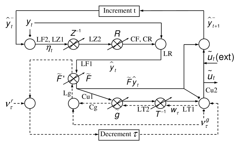
Figure 6: Block diagram of full NN algorithm. Each $\bigcirc$ block combines inputs; arrowhead inputs are added, filled-circle inputs are subtracted. Each $\otimes$ block multiplies its input by the matrix indicated alongside the block. An arrow through a block denotes a matrix to be learned. The solid path implements KF learning and execution, and KC execution; the dashed path, KC learning. Link symbols are as in Fig. 1.

The solid-line portion of Fig. 6 shows the signal flow that integrates Kalman estimation (KF execution and learning), system identification, and KC execution. Assume for now that line Cu1 and/or Cu2 is cut; i.e., no control signals are computed. For the Kalman estimation (KF) execution process, starting with the link (near upper left) labeled $\eta_{t}$, the computation sequence is (cf. Eq. 12): $\eta_{t}\rightarrow Z^{-1}\eta_{t}\rightarrow RZ^{-1}\eta_{t}\rightarrow\hat{y}_{t}=y_{t}+RZ^{-1}\eta_{t}\rightarrow\tilde{F}\hat{y}_{t}\rightarrow\hat{y}^{-}_{t+1}=\tilde{u}_{t}({\rm ext})+\tilde{F}\hat{y}_{t}\rightarrow\eta_{t+1}=-y_{t+1}+\hat{y}^{-}_{t+1}$ [external driving term $\tilde{u}_{t}({\rm ext})$ is optional]. Using Method 1 of section 3.3 (Eq. 16), $Z$ learning occurs at link LZ1; or, using Method 2 (Eq. 17), $Z^{-1}$ learning occurs at link LZ2. $\tilde{F}$ learning (Eq. 20) uses $\hat{y}_{t-1}$ at link LF1 (held from the previous time step $t-1$) and $\eta_{t}$ at link LF2. For initial learning of $\tilde{F}$ (before $Z$ is used; cf. Eq. 18), the circuit is cut at link CF, so that LF1 carries activity $y_{t-1}$ and LF2 carries $\epsilon_{t}=\tilde{F}_{t-1}y_{t-1}+\tilde{u}_{t-1}-y_{t}$. In the ‘offline sensor’ mode for learning $R$ (cf. section 3.5.2), the circuit is cut at link CR, so that the following link LR carries activity $y_{t}=n_{t}$.

Execution of control is shown in Fig. 6 (solid path) starting at link Cu1. The computation sequence (cf. Eq. 25) is: $\tilde{F}\hat{y}_{t}\rightarrow\tilde{g}\tilde{F}\hat{y}_{t}\rightarrow T^{-1}\tilde{g}\tilde{F}\hat{y}_{t}\rightarrow\tilde{u}_{t}=-\tilde{F}\hat{y}_{t}+T^{-1}\tilde{g}\tilde{F}\hat{y}_{t}=(-I+T^{-1}\tilde{g})\tilde{F}\hat{y}$ at link Cu2. Output $\tilde{u}_{t}$ is the control signal, and is also provided as efferent-copy feedback to compute $\hat{y}^{-}_{t+1}$.

The dashed portion of Fig. 6 shows the signal flows that implement learning of control; i.e., $w$ evolution and the learning of $T$ (or $T^{-1}$) and $\tilde{g}$. For $w$ evolution (Eq. 24), the computation sequence is (starting near lower right, at the link labeled $w_{\tau}$): $w_{\tau}\rightarrow T^{-1}w_{\tau}\rightarrow\tilde{g}T^{-1}w_{\tau}\rightarrow\nu^{g}_{\tau}+\tilde{g}T^{-1}w_{\tau}\rightarrow\tilde{F}^{\prime}(\nu^{g}_{\tau}+\tilde{g}T^{-1}w_{\tau})\rightarrow\nu^{r}_{\tau}+\tilde{F}^{\prime}(\nu^{g}_{\tau}+\tilde{g}T^{-1}w_{\tau})\rightarrow w_{\tau-1}=-\nu^{g}_{\tau-1}+\nu^{r}_{\tau}+\tilde{F}^{\prime}(\nu^{g}_{\tau}+\tilde{g}T^{-1}w_{\tau})$.

Either $T$ learning occurs at link LT1, or $T^{-1}$ learning occurs at link LT2 (cf. Eq. 26 and just above it). The $\tilde{F}^{\prime}$ connections will join the same nodes as $\tilde{F}$, but in the reverse direction (discussed below); thus they are learned along with $\tilde{F}$ (prior to being used for control) using the same Hebb rule (Eq. 18 or 20). Matrix $\tilde{g}$ is learned (analogously to $R$ above) in a mode of circuit operation in which the dashed link Cg is cut, so that the next link Lg carries activity $\nu^{g}_{\tau}$, which is used for Hebbian learning of $\tilde{g}=E[\nu^{g}(\nu^{g})^{\prime}]$. (Cf. section 4, paragraph starting ‘Learning of $\tilde{g}$ …’.)

The circuit of Fig. 6 operates switchably in several distinct modes, each using a portion of the circuit with cuts (breaks in signal flow) as described. At start-up: Learn $\tilde{F}$ and $\tilde{F}^{\prime}$; this circuit mode has a cut at CF, with signal flow along solid path. Learn $R$ using offline sensor operation (no external input); this mode uses solid path with cut at CR. Then, for each (increasing) $t$:

1. Perform KF learning & execution (solid path). If not also performing KC, the KF mode has a cut at Cu1 or Cu2. If performing KC:

   1. If KC matrix for this $t$ has been stored, retrieve it. Otherwise: learn $\tilde{g}$ (mode: dashed path, cut at Cg) if not already done; iterate $\tau$ from goal-completion time $N$ backward to $t$ (mode: dashed path, $t$ held constant while $\tau$ is decremented); and optionally store intermediate KC matrices.

   2. KC execution: Use KC matrix to calculate $\tilde{u}$ (mode: solid path), and provide efferent copy to KF.

2. Optionally update $\tilde{F}$ and $\tilde{F}^{\prime}$ during KF operation (mode: solid path, no cut at CF).

3. Optionally update $R$ (‘offline sensor’ mode: CR cut, solid path).

Appendix C. Comments on a recent KF-inspired NN algorithm

In a recent paper, Szirtes, Póczos, & Lőrincz (2005) (hereafter referred to as ‘SPL’) observe: ‘Connectionist representation of [Kalman filter-like] mechanisms with Hebbian learning rules has not yet been derived.’ They state: ‘The first problem of the classical [Kalman] solution is that covariance matrices of [the plant and measurement] noises are generally assumed to be known. The second problem is that …the algorithm requires the calculation of a matrix inversion, which is hard to interpret in neurobiological terms. [Here] we derive an approximation of the Kalman gain, which eliminates these problems.’

In this section we show that the sequence of alterations made by SPL to the KF equations is not well-justified, and that the SPL simulations, which show a reduction of prediction error with time, do not provide evidence that their algorithm is in fact computing an approximation of the optimal Kalman gain.

SPL denotes the ‘Kalman gain’ matrix by $K^{t}$, which corresponds to our $FK_{t}$ (cf. our Eq. 3 and their Eq. 3). At the outset, their stated goal is actually not to compute the Kalman-optimal $K^{t}$. Instead, they consider only a family of matrices, which we will denote $\tilde{K}(\theta)$, parametrized by a vector $\theta$, for which the elements of $\tilde{K}(\theta)$ are $\tilde{K}_{ij}(\theta)\equiv K_{ij}\theta_{i}$ for each column $i$, where $K$ is a given and fixed arbitrary matrix. SPL’s goal is to adaptively learn $\theta$ over time, using a NN algorithm, so that its final learned value $\theta^{*}$ has the property that $\tilde{K}(\theta^{*})$ minimizes the prediction error over the family of all possible $\tilde{K}(\theta)$. Since $K$ is arbitrary, the parametrized family of matrices may not include (or even contain a matrix that approximates) the actual optimal KF. (Note that if $K^{t}$ is an $N\times N$ matrix, the set of all possible $K^{t}$ is being replaced by a family parametrized by $\theta$, which has only $N$, not $N^{2}$, components.)

Given this goal, the first step in the SPL derivation is to minimize the prediction error by performing stochastic gradient descent. This yields a pair of equations for $\theta^{t+1}_{k}$ and an auxiliary matrix $W^{t+1}_{ik}$, in terms of values at time $t$:

$$\theta^{t+1}_{k}=\theta^{t}_{k}+\alpha\Sigma_{lj}K_{kl}H_{lj}W_{jk}\epsilon^{t}_{k}~{};$$ (35)

$$W^{t+1}_{ik}=\Sigma_{j}F_{ij}W^{t}_{jk}-\theta^{t}_{i}\Sigma_{lj}K_{il}H_{lj}W^{t}_{jk}+\delta_{ik}\epsilon^{t}_{k}~{}.$$ (36)

To obtain their model ’O1’ (SPL Eqs. 5-6), SPL introduces a random vector $\xi$, which ‘can be regarded as sparse, internally generated noise,’ in order ‘to provide a conventional neuronal equation.’ In SPL Eq. 6, the first two right-hand terms are accordingly equal to $\xi_{k}$ times the corresponding terms of the above Eq. 36. This multiplication by $\xi_{k}$ is, however, not justified. If, for example, $\xi$ has zero mean (actually the $\xi$ distribution is nowhere specified), each of those two (now incorrect) terms will average to zero, and will thus make no contribution, on average, to $W^{t+1}_{ik}$. Therefore model ‘O1’ is not a valid approximation.

Several additional alterations are then made to generate a succession of SPL models called ‘O2’ through ‘O5.’

To obtain model ‘O2’ (SPL Eqs. 7-8), SPL writes ‘to simplify the complexity of the iteration, we may suppose that the system is near optimal: $K\approx H^{-1}$.’ Since the $K$ referred to here is the arbitrary and fixed $K$ that enters the above definition of $\tilde{K}(\theta)$, one is free to choose $K\approx H^{-1}$, or even $K=H^{-1}$, irrespective of whether ‘the system is near optimal.’ However, doing so in no way ensures that the learned $\theta$ will yield a $\tilde{K}$ that is approximately Kalman-optimal. Certainly the optimal KF is not in general approximately equal to $H^{-1}$; it may be quite far from this value, depending upon $F$ and the relationship between the plant and measurement noise covariances. This (as well as some of the following points) can be most easily confirmed by considering the simple 1-d case, in which all matrices are scalar quantities.

To obtain model ‘O3’ (SPL Eqs. 9-10), SPL states that because only diagonal elements $W_{kk}$ enter SPL Eq. 8 for the evolution of $\theta$, therefore ‘we may neglect the off-diagonal elements of matrix $W$ in Eq. 7’ (the evolution equation for $W$). However, such neglect will introduce errors into the diagonal elements of $W$, and thereby into the evolution of $\theta$.

To obtain model ‘O4’ (SPL Eqs. 11-12), SPL writes that a ‘further simplification neglects the self-excitatory contribution, $F_{ii}W^{t}_{ii}\xi_{i}$.’ However, this term is not in general small compared with the remaining terms.

Finally, to obtain model ‘O5’ (SPL Eqs. 13-14), SPL introduces the ‘stabilized form’ of model ‘O4.’ This means that instead of setting $W^{t+1}$ equal to a specified function $f(W^{t})$, as in model ‘O4,’ SPL re-defines $W^{t+1}$ as $W^{t+1}=W^{t}+\gamma f(W^{t})$, where $\gamma$ is a (presumably small) learning rate. At this step, it would have been more appropriate to define instead $W^{t+1}=(1-\gamma)W^{t}+\gamma f(W^{t})$, so that if $W^{t+1}=W^{t}$ in model ‘O4,’ it would do so in model ‘O5’ as well.

Thus each of models ‘O1’ through ‘O5’ is obtained by making an alteration or simplification that is not a justified approximation to the previous model, nor to the original stochastic gradient form given by our Eqs. 35 and 36 above.

SPL then presents simulations (SPL Fig. 1) that show a rapid decrease in prediction error $\parallel x-\hat{x}\parallel$ (their $\hat{x}$ is our $\hat{x}^{-}$), and in the related ‘reconstruction error’, $\parallel y-H\hat{x}\parallel$, with time. This is stated to be a ‘comparison of direct [i.e., classical solution] and approximated Kalman filters.’ However, it can easily be seen that even if one combines the prediction from the previous time step with the current measurement by using a blending matrix ($K^{t}$ in SPL’s Eq. 3) that is arbitrary and fixed, the prediction error starting with an initial arbitrary guess – prior to making any measurements on the system – will at first rapidly (exponentially) decrease as more measurements are made. (This is true provided only that $K^{t}$ is such that the posterior estimate of $x^{t}$ tends to move toward, rather than away from, $H^{-1}y^{t}$; i.e., provided that $K^{t}$ actually blends the new measurement with the prior prediction, rather than repelling the predicted $H\hat{x}$ away from the new measurement.)

SPL does not display the $\tilde{K}(\theta)$ that is learned using their algorithm, so one cannot tell whether or how that matrix converges to an approximation of the optimal Kalman filter. The asymptotic prediction errors obtained using (a) the optimal KF, (b) an arbitrary fixed KF, and (c) a KF that varies according to an arbitrary algorithm, will, subject to the proviso above, typically differ by a modest factor as long as the plant and measurement SNRs differ by only 8 dB as in SPL’s simulation. Thus the differences in asymptotic error are not visible on the scale of SPL’s Fig. 1, in which initial errors are huge (simply because the initial prediction is a guess made in the absence of prior measurements) compared with the asymptotic errors using any of these blending matrices.

It is also worth noting that the learning rate $\alpha=0.01$ is held constant in SPL’s simulation (according to the SPL Fig. 1 caption). However, a rate factor that is appropriate initially, when prediction errors are huge, must be increased substantially as prediction errors decrease, in order to ensure that learning continues. This raises the possibility that SPL learning may have stalled early in the simulation, although one cannot tell without seeing the evolution of $\theta$ or $\tilde{K}(\theta)$ with time. Even if $\alpha$ had been adaptively altered to avoid such stalling, however, the above discussion shows that the claim of approximately optimal KF learning using SPL’s ‘O1’ through ‘O5’ algorithms is not warranted, and that the comparison of predicted errors vs. time in SPL’s Fig. 1 does not indicate that KF-like learning has occurred.

Appendix D. An alternative ‘mapping’ between the KPC NN and the LCC

To see what happens if we consider a mapping that is more detailed than I think is warranted in view of the caveats in Section 5, we can modify Dgm. D1 to obtain Dgm. D3:

R	$\rightarrow$	g	$\rightarrow$	T	$\rightarrow$	Z	$\rightarrow$ R
$\uparrow$		$\downarrow$		$\downarrow$		$\uparrow$
$y$		$(\tilde{F}\hat{y})$		$\tilde{u}$		$y$	[D3]

Additional direct g $\rightarrow$ Z and Z $\rightarrow$ g paths (Fig. 4a) are omitted from D3 for notational simplicity. KC learning adds paths T $\rightarrow$ g $\rightarrow$ R (Fig. 4b).

On this view, one might then posit a one-to-one correspondence between NN layers {R, g, T, Z} and LCC layers {4, 2/3, 5, 6}, respectively. Then an exact match would imply the existence of LCC paths $4\rightarrow 2/3\rightarrow 5\rightarrow 6\rightarrow 4$, $5\rightarrow 2/3$ (used for KC learning in the NN), and $2/3\rightarrow 6$, and with input from a ‘lower’ cortical area (or thalamus) to 4 and 6, output from 5 to a lower area, and output from 2/3 to the same or a higher area. All of these paths fit within current understanding of LCC connectivity (Callaway, 1998; Douglas & Martin, 2004; Gilbert, 1983; Raizada & Grossberg, 2001). An exact match would, however, also imply LCC paths $6\rightarrow 2/3\rightarrow 4$. The $6\rightarrow 2/3$ path has been described (Hirsch et al., 1998), but in the context of V1 complex-cell interconnections. Also, NN layer g is used only for KC (and as a layer through which $\tilde{F}\hat{y}$ passes (Fig. 4a)), arguing against identifying layer g with LCC layer 2/3, which is important in sensory processing. I thus expect the less-detailed resemblance between Dgms. D1 and D2 to be more robust than that between D3 and D2, as more complex prediction and control tasks, and different sets of allowed NN operations, are studied in future work.

References

Becker, S. & Hinton, G. E. (1992). Self-organizing neural network that discovers surfaces in random-dot stereograms. Nature, 355, 161-163.

Callaway, E. M. (1998). Local circuits in primary visual cortex of the macaque monkey. Annu. Rev. Neurosci., 21, 47-74.

Douglas, R. J. & Martin, K. A. C. (2004). Neuronal circuits of the neocortex. Annu. Rev. Neurosci., 27, 419-51.

George, D. & Hawkins, J. (2005). A hierarchical Bayesian model of invariant pattern recognition in the visual cortex. Proc. 2005 IEEE Int. Joint Conf. Neural Networks, 3, 1812-17.

Gilbert, C. D. (1983). Microcircuitry of the visual cortex. Annu. Rev. Neurosci., 6, 217-247.

Grossberg, S. & Williamson, J. R. (2001). A neural model of how horizontal and interlaminar connections of visual cortex develop into adult circuits that carry out perceptual grouping and learning. Cerebral Cortex, 11, 37-58.

Haykin, S. (1999) Neural Networks: A Comprehensive Foundation, 2nd ed. (Prentice Hall).

Haykin, S. (2001) Kalman Filtering and Neural Networks (Wiley-Interscience); especially chap. 2, pp. 23-68 by Puskorius, G. V. & Feldkamp, L. A. Parameter-based Kalman filter training: Theory and implementation.

Hertz, J., Krogh, A., & Palmer, R. G. (1991) Introduction to the Theory of Neural Computation (Addison-Wesley).

Hinton, G. E. & Ghahramani, Z. (1997). Generative models for discovering sparse distributed representations. Philos. Trans. R. Soc. London, B, 352, 1177-90.

Hinton, G. E., Osindero, S. & Teh, Y. (2006). A fast learning algorithm for deep belief nets. Neural Computation, 18, 1527-1554.

Hirsch, J. A., Gallagher, C. A., Alonso, J.-M., & Martinez, L. M. (1998). Ascending projections of simple and complex cells in layer 6 of the cat striate cortex. J. Neurosci., 18, 8086-94.

Kalman, R. E. (1960). A new approach to linear filtering and prediction problems. Trans. ASME – J. Basic Eng., 82, 35-45.

Klimasauskas, C. C. & Guiver, J. P. (2001). Hybrid linear – neural network process control. U.S. Patent #6278962.

Körding, K. P. & Wolpert, D. M. (2004). Bayesian integration in sensorimotor learning. Nature, 427, 244-47.

Lee, T. S. & Mumford, D. (2003). Hierarchical Bayesian inference in the visual cortex. J. Opt. Soc. Am. A, 20, 1434-48.

Lewicki, M. S. & Sejnowski, T. J. (1997). Bayesian unsupervised learning of higher order structure. Adv. Neural Info. Proc. Systems, 9, 529-35.

Linsker, R. (1992). Local synaptic learning rules suffice to maximize mutual information in a linear network. Neural Computation, 4, 691-702.

Linsker, R. (2005). Improved local learning rule for information maximization and related applications. Neural Networks, 18, 261-265.

Mountcastle, V. B. (1998). Perceptual neuroscience: the cerebral cortex (Harvard Univ. Press).

Murata, N., Müller, K.-R., Ziehe, A., & Amari, S.-i. (1997). Adaptive on-line learning in changing environments. Adv. Neural Info. Proc. Systems, 9, 599-605.

Poggio, T. & Bizzi, E. (2004). Generalization in vision and motor control. Nature, 431, 768-74.

Raizada, R. D. S. & Grossberg, S. (2001). Context-sensitive binding by the laminar circuits of V1 and V2: A unified model of perceptual grouping, attention, and orientation contrast. Visual Cognition, 8, 431-466; see refs. cited in Table 1.

Rao, R. P. N. (1999). An optimal estimation approach to visual perception and learning. Vision Res., 39, 1963-89.

Rao, R. P. N. (2004). Bayesian computation in recurrent neural circuits. Neural Computation, 16, 1-38.

Rao, R. P. N. (2005). Bayesian inference and attentional modulation in the visual cortex. NeuroReport, 16, 1843-48.

Rao, R. P. N. & Ballard, D. H. (1997). Dynamic Model of Visual Recognition Predicts Neural Response Properties in the Visual Cortex. Neural Computation, 9, 721-63.

Rieke, F., Warland, D., de Ruyter van Steveninck, R., & Bialek, W. (1999). Spikes: Exploring the Neural Code (MIT Press).

Rivals, I. & Personnaz, L. (1998). A recursive algorithm based on the extended Kalman filter for the training of feedforward neural models. Neurocomputing, 20, 279-94.

Singhal, S. & Wu, L. (1989). Training Multilayer Perceptrons with the Extended Kalman Algorithm. Advances in Neural Information Processing Systems, 1, 133-140.

Szirtes, G., Póczos, B., & Lőrincz, A. (2005). Neural Kalman-filter. Neurocomputing, 65-66, 349-355.

Szita, I. & Lőrincz, A. (2004). Kalman filter control embedded into the reinforcement learning framework. Neural Computation, 16, 491-499.

Todorov, E. (2005). Stochastic optimal control and estimation methods adapted to the noise characteristics of the sensorimotor system. Neural Computation, 17, 1084-1108.

Tresp, V. (2001). Method and arrangement for the neural modelling of a dynamic system with non-linear stochastic behavior. U. S. Patent #6272480.

Williams, R. J. (1992). Training recurrent networks using the extended Kalman filter. In: Proceedings of the International Joint Conference on Neural Networks, June, 1992, Baltimore, MD, Vol. IV, pp. 241-246.

Yu, A. J. & Dayan, P. (2005). Inference, attention, and decision in a Bayesian neural architecture. Adv. Neural Info. Proc. Systems, 17, 1577-84.

Zemel, R. S., Huys, Q. J. M., Natarajan, R., & Dayan, P. (2005). Probabilistic computation in spiking populations. Adv. Neural Info. Proc. Systems, 17, 1609-16.