Abstract

Employing a novel type of non-commutative product in the Dirac-Kähler twisted superspace on a lattice, we formulate a field theoretically rigid framework of extended supersymmetry on a lattice. As a first example of this treatment, we calculate one-loop (in some cases any loops) quantum corrections for a twisted Wess-Zumino model with $N\times N$ hermitian matrix superfields on a two dimensional lattice. The calculations are entirely given in a lattice superfield framework. We report that the mass and the coupling constant are exactly protected from the radiative corrections at non-zero lattice spacing as far as the planar diagrams are concerned, which implies the realization of exact lattice supersymmetry w.r.t. all the supercharges in the large-$N$ limit.

1 Introduction

There have been a variety of studies addressing the subject of supersymmetry (SUSY) on a lattice. The literal purpose of lattice SUSY is to provide a well-defined constructive framework of SUSY formulations with which one may extract the fully non-perturbative information either analytically or numerically. A successful formulation of lattice SUSY may be expected to provide a deeper understanding of the relationship between bosons and fermions in a regularized framework. In recent years, it has been recognized that the so-called twisted SUSY formulations are playing particularly important roles in this challenging subject [1, 2, 3, 4, 5, 6]. It was also recently pointed out that amongst the other formulations of lattice SUSY [7], the deconstruction formulation [8] is quite closely related to the twisted SUSY formulation on the lattice [9]. In spite of these developments, however, realizing all the SUSY generators in a SUSY algebra being considered, say, $D=4\ \mathcal{N}=1$ or $D=2\ \mathcal{N}=2$ or whatever , exactly on a lattice, has been considered as a very non-trivial task. This is essentially because in general only the finite subgroup of the entire translational symmetry group in the continuum spacetime can be survived at non-zero lattice spacings.

In the series of papers [1, 2, 3], we have proposed an extended SUSY formulation on a lattice which keeps all the SUSY transformations exact at least at classical level. The formulation is based on the two crucial theoretical ingredients. The one is the notion of twisted SUSY. This is essentially originated from the intrinsic relation between twisted fermions and staggered fermions or more appropriately Dirac-Kähler fermions [10]. It has been pointed out that the fermionic components in the lattice SUSY multiplet are realized as a staggered fermion, and accordingly the spectrum doubling turns to have a physically relevant meaning as an extended SUSY degrees of freedom [1]. The lattice fermions in this framework have their own geometrical meaning. They have one-to-one correspondence with all the simplices available on a lattice being considered, namely, 0, 1 and 2-form on a two dimensional lattice or 0, 1, 2, 3 and 4-form on a four dimensional lattice, which is a natural consequence of the Dirac-Kähler fermion realization on a lattice [11]. The other crucial ingredient, which is also tightly related to the Dirac-Kähler structure, is the “mild” non-commutativity associated with the lattice supercharges. It has been long recognized that the breakdown of Leibniz rule is one of the major obstacles in realizing exact SUSY on a lattice. The notion of “mild” non-commutativity has been introduced in order to overcome this difficulty. The non-commutative nature of lattice supercharges can be trace back to the intrinsic non-commutative property of difference operators. In [1], we have shown that if the non-commutativity matching conditions, which we refer to as the Leibniz rule conditions on a lattice, are satisfied, then all the supercharges can be exactly realized on the lattice at least at classical level. This notion of “mild” non-commutativity has been further applied to the formulations of extended supersymmetric gauge theories by means of link supercharges and link component fields [2, 3] and recently also applied to the formulation of Chern-Simons theory on a three dimensional lattice [12].

In spite of these developments, on the other hand, we have not addressed the quantum aspects of these formulations so far since it has not been fully established how to deal with the above “mild” non-commutativity in a quantum field theoretically rigid manner. In this paper, we attack this problem and propose a field theoretically well-defined treatment of the “mild” non-commutative SUSY formulation on a lattice. In particular, we shall employ a novel type of non-commutative product in the Dirac-Kähler twisted superspace which honestly accommodates the “mild” non-commutativity introduced in Ref. [1]. As a first example of this framework, we shall calculate one-loop (in some cases any loops) quantum corrections for a twisted Wess-Zumino model with $N\times N$ hermitian matrix superfields on a two dimensional lattice. The calculations are entirely given in the lattice superfield method. We report that the mass and the coupling constant are exactly protected from the quantum corrections as far as the planar diagrams are concerned, while the SUSY spoiling non-planar contributions are suppressed at least by $\mathcal{O}(a^{2}/N)$. These features imply the realization of exact lattice supersymmetry w.r.t. all the supercharges in the ’t Hooft large-$N$ limit.

This paper is organized as follows. In Sec. 2, after introducing a novel type of non-commutative product which honestly represents the “mild” non-commutativity which we have introduced in [1], we (re-)formulate the lattice counterpart of extended SUSY algebra and see how to construct an extended SUSY invariant action on a lattice. In Sec. 3, as a simple and explicit example, we introduce the Dirac-Kähler twisted $\mathcal{N}=D=2$ SUSY algebra and explicitly see how the lattice SUSY algebra is realized in accordance with the lattice Leibniz rule conditions. We then construct a $\mathcal{N}=D=2$ twisted Wess-Zumino model on a lattice and proceed to derive the superfield propagators and the three-point vertex functions, taking a full advantage of the lattice superfield method. In Sec. 4, we extend the chiral and anti-chiral superfields introduced in Sec. 3 to $N\times N$ hermitian matrix valued superfields in order to set up the $\mathcal{N}=D=2$ twisted Wess-Zumino model with global $U(N)$ symmetry. We perturbatively investigate the possible radiative corrections to this model by explicitly calculating the one-loop (in some cases any loops) contributions to the kinetic term, the mass term and the interaction term of the lattice action. We then find out that the quantum corrections strictly protect the lattice SUSY as far as the planar diagrams are concerned. In particular, we shall see that apart from the overall wave function renormalization the mass and the coupling constant are strictly protected (at least to this order) from the radiative corrections in the planar diagrams. These features imply the full realization of exact SUSY at non-zero lattice spacing in the ’t Hooft large-$N$ limit. Sec. 5 summarizes the formulation with some discussions.

2 Introducing a Non-Commutative Product

In this section, we first introduce a novel non-commutative product in the Dirac-Kähler twisted superspace which honestly represent the “mild” non-commutativity introduced in Ref. [1] and present how to formulate a lattice counterpart of SUSY algebra. The non-commutativity introduced in Ref [1] in order to keep the lattice Leibniz rule is the one between the bosonic (discrete) coordinate $x_{\mu}$ and Grassmann coordinate $\theta_{A}$ in the twisted superspace $(x_{\mu},\theta_{A})$,

$$\theta_{A}f(x)=(-1)^{|f|}f(x-2a_{A})\theta_{A},$$ (2.1)

or equivalently,

$$[x_{\mu},\theta_{A}] = 2(a_{A})_{\mu}\theta_{A},$$ (2.2)

where the symbol $|f|$ takes value of $+1$ or $-1$ for the bosonic or fermionic function $f$, respectively. $\theta_{A}$ is representing any fermionic coordinate in the Dirac-Kähler twisted superspace, namely, $\theta_{A}=(\theta,\theta_{\mu},\tilde{\theta})$ with $\mu=1,2$ in $\mathcal{N}=D=2$ [1, 2], $\theta_{A}=(\theta,\theta_{\mu},\overline{\theta}_{\mu},\overline{\theta})$ with $\mu=1\sim 3$ in $\mathcal{N}=4\ D=3$ [3] and $\theta_{A}=(\theta,\theta_{\mu},\theta_{\mu\nu},\tilde{\theta}_{\mu},\tilde{\theta})$ with $\mu,\nu=1\sim 4$ in $\mathcal{N}=D=4$ [2]. The vector $a_{A}$ in the r.h.s. of (2.2) governing the non-commutativity between $x_{\mu}$ and $\theta_{A}$ is to be constrained at a later stage such that the resulting SUSY algebra be consistent with the non-commutativity matching conditions which we refer to as the lattice Leibniz rule conditions. In this framework, superfields may generically be expanded in terms of the non-commutative $\theta_{A}$’s such as

$$\Phi(x,\theta_{A}) = \phi(x)+\theta_{A}\phi_{A}(x+a_{A})+\theta_{A}\theta_{B}\phi_{AB}(x+a_{A}+a_{B})+\cdots,$$ (2.3)

$$= \phi(x)+(-1)^{|\phi_{A}|}\phi_{A}(x-a_{A})\theta_{A}+\phi_{AB}(x-a_{A}-a_{B})\theta_{A}\theta_{B}+\cdots,$$ (2.4)

where the component fields are chosen to be located in a symmetric manner. The symbol $|\phi|$ again takes the value $+1(-1)$ for the bosonic (fermionic) component field $\phi$. All the superfield operators such as supercharges and supercovariant derivatives are accordingly represented in terms of the non-commutative $\theta_{A}$’s on the lattice. The highlight of the formulation based on the relation (2.2) is that the resulting lattice action can be manifestly invariant under all the SUSY variations at least at tree level if the lattice Leibniz rule conditions are satisfied [1]. On the other hand, it is rather non-trivial how to deal with the non-commutativity (2.2) within the framework of quantum field theory. One possible way to provide a field theoretically more rigid framework is to formulate the bosonic and fermionic coordinates entirely in terms of matrix representations and deal with the (super)fields as the functions of these (super)coordinate matrices. A formulation presented in Ref. [6] may be placed along this direction.

A somewhat alternative way to treat the non-commutativity (2.2), which is our starting point of this paper, is to alter the notion of product and introduce a non-commutative product in such a way to satisfy the relation,

$$[x_{\mu},\theta_{A}]_{*}\ \equiv\ x_{\mu}*\theta_{A}-\theta_{A}*x_{\mu} = 2(a_{A})_{\mu}\theta_{A}.$$ (2.5)

This type of non-commutativity treatment may be regarded as a certain analogue of the Moyal star product whose quantum implications have been extensively investigated (e.g. [13] for a review). The principle we shall take is that all the non-commutativity should be originated from the nature of the product denoted as $*$ in (2.5), while the $x_{\mu}$ and $\theta_{A}$ should be treated as the ordinary (discrete) bosonic coordinates and fermionic coordinates, respectively. In this framework, superfields can be expanded in terms of ordinary fermionic coordinates and ordinary functions,

$$\Phi(x,\theta_{A}) = \phi(x)+\theta_{A}\phi_{A}(x)+\theta_{A}\theta_{B}\phi_{AB}(x)+\cdots,$$ (2.6)

and thus may be served as path integration variables such as in the standard SUSY treatment in the continuum spacetime [14, 15, 16, 17]. A star product of superfields, which is intrinsically non-commutative, is defined in terms of $*$ subject to the relation (2.5),

$$\Phi_{1}(x,\theta_{A})*\Phi_{2}(x,\theta_{B})\neq\Phi_{2}(x,\theta_{B})*\Phi_{1}(x,\theta_{A}).$$ (2.7)

An explicit representation of the star product satisfying the relation (2.5) may be given by

$$\Phi_{1}(x,\theta_{A})*\Phi_{2}(x,\theta_{B})\equiv\mu(\mathcal{F}^{-1}_{L}\mathcal{F}_{R}\ \Phi_{1}(x,\theta_{A})\otimes\Phi_{2}(x,\theta_{B})),$$ (2.8)

with the elements $\mathcal{F}_{L}$ and $\mathcal{F}_{R}$,

$$\mathcal{F}_{L} = \exp\{{\sum_{\rho}\sum_{A}(a_{A})_{\rho}\theta_{A}\frac{\partial}{\partial\theta_{A}}\otimes\partial_{\rho}}\},\hskip 20.0pt\mathcal{F}_{R}\ =\ \exp\{{\sum_{\rho}\partial_{\rho}\otimes\sum_{A}(a_{A})_{\rho}\theta_{A}\frac{\partial}{\partial\theta_{A}}}\},\qquad$$ (2.9)

where in (2.8) the symbol $\mu$ denotes the multiplication map, $\mu(f\otimes g)\equiv fg$. The operator $\theta_{A}\frac{\partial}{\partial\theta_{A}}$ in the r.h.s.’s of (2.9) should be understood as an adjoint operation,

$$\theta_{A}\frac{\partial}{\partial\theta_{A}}adj\ \theta_{A}\frac{\partial}{\partial\theta_{A}}=[\theta_{A}\frac{\partial}{\partial\theta_{A}},\ ],$$ (2.10)

together with the anti-commutation relation between $\frac{\partial}{\partial\theta_{A}}$ and $\theta_{B}$,

$$\{\frac{\partial}{\partial\theta_{A}},\theta_{B}\}=\delta_{AB}.$$ (2.11)

One may easily verify that the elements $\mathcal{F}^{-1}_{L}$ and $\mathcal{F}_{R}$ independently give rise to the following relations,

$$\mu(\mathcal{F}^{-1}_{L}\ \theta_{A}\otimes f(x)) = \theta_{A}f(x-a_{A}),\hskip 20.0pt\mu(\mathcal{F}^{-1}_{L}\ f(x)\otimes\theta_{A})\ =\ f(x)\theta_{A},$$ (2.12)

$$\mu(\mathcal{F}_{R}\ \theta_{A}\otimes f(x)) = \theta_{A}f(x),\hskip 54.0pt\mu(\mathcal{F}_{R}\ f(x)\otimes\theta_{A})\ =\ f(x+a_{A})\theta_{A}.$$ (2.13)

Accordingly, the star product defined in (2.8) would give,

$$\theta_{A}*f(x) = \theta_{A}f(x-a_{A}),\hskip 20.0ptf(x)*\theta_{A}\ =\ f(x+a_{A})\theta_{A}.$$ (2.14)

It is now obvious that the relation (2.5) is satisfied just by taking $f(x)=x$. It is important to notice that the star product (2.8) satisfies the associativity,

$$\bigl{(}\Phi_{1}(x,\theta_{A})*\Phi_{2}(x,\theta_{B})\bigr{)}*\Phi_{3}(x,\theta_{C}) = \Phi_{1}(x,\theta_{A})*\bigl{(}\Phi_{2}(x,\theta_{B})*\Phi_{3}(x,\theta_{C})\bigr{)}.$$ (2.15)

Also note that the star product of the super derivative operators $\frac{\partial}{\partial\theta_{A}}$ gives rise to the opposite shifts compared to (2.14),

$$\frac{\partial}{\partial\theta_{A}}*f(x) = \frac{\partial}{\partial\theta_{A}}f(x+a_{A}),\hskip 20.0ptf(x)*\frac{\partial}{\partial\theta_{A}}\ =\ f(x-a_{A})\frac{\partial}{\partial\theta_{A}},$$ (2.16)

with which one can verify that the anti-commutation relation (2.11) holds also in the star product language,

$$\{\frac{\partial}{\partial\theta_{A}},\theta_{B}\}*f(x) \equiv \frac{\partial}{\partial\theta_{A}}*\theta_{B}*f(x)+\theta_{B}*\frac{\partial}{\partial\theta_{A}}*f(x)\ =\ \delta_{AB}f(x).$$ (2.17)

Although the combination of the elements $(\mathcal{F}^{-1}_{L})^{t}(\mathcal{F}_{R})^{2-t}$ with an arbitrary parameter $t$ would always induce a non-commutative product which satisfies the relation (2.5), in this paper we shall only consider the symmetric definition given in (2.8).

Having introduced a non-commutative product between the bosonic and fermionic coordinate of the superspace, $x_{\mu}$ and $\theta_{A}$, we also require the same amount of non-commutativity between $x_{\mu}$ and Grassmann parameters $\xi_{A}$,

$$\xi_{A}*f(x) = \xi_{A}f(x-a_{A}),\hskip 20.0ptf(x)*\xi_{A}\ =\ f(x+a_{A})\xi_{A},$$ (2.18)

such that the operation of $\xi_{A}\frac{\partial}{\partial\theta_{A}}$ would properly induce a derivative w.r.t. $\theta_{A}$ also in the language of the star product,

$$\biggl{[}\xi_{A}\frac{\partial}{\partial\theta_{A}},\phi(x)+\theta_{B}\phi_{B}(x)+\cdots\bigg{]}_{*} \equiv \xi_{A}\frac{\partial}{\partial\theta_{A}}*\bigl{(}\phi(x)+\theta_{B}\phi_{B}(x)+\cdots\bigr{)}$$ (2.19)

$$-\bigl{(}\phi(x)+\theta_{B}\phi_{B}(x)+\cdots\bigr{)}*\xi_{A}\frac{\partial}{\partial\theta_{A}}$$

$$= \delta_{AB}\xi_{A}\phi_{B}(x)+\cdots.$$

This extension can easily be done by just replacing the $\theta_{A}\frac{\partial}{\partial\theta_{A}}$ as $\xi_{A}\frac{\partial}{\partial\xi_{A}}+\theta_{A}\frac{\partial}{\partial\theta_{A}}$ in the expressions (2.9).

Based on the above setup, we now proceed to define a lattice counterpart of SUSY algebra. Since in the continuum spacetime, SUSY algebra can be regarded as a fermionic decomposition of differential operators, one may naturally expect that a lattice counterpart of SUSY algebra can be formally expressed as a fermionic decomposition of difference operators,

$$\{Q_{A},Q_{B}\} = f^{\mu}_{AB}d_{\mu},$$ (2.20)

where $f^{\mu}_{AB}$ denotes a numerical coefficient, while $d_{\mu}$ denotes a “formal” difference operator to be specified in the following. A SUSY transformation on the lattice is defined by a $*$ commutator between a supercharge $Q_{A}$ associated with a corresponding Grassmann parameter $\xi_{A}$ and a superfield $\Phi(x,\theta_{C})$,

$$\delta_{A}\Phi(x,\theta_{C}) \equiv [\xi_{A}Q_{A},\Phi(x,\theta_{C})]_{*}$$ (2.21)

$$= \xi_{A}Q_{A}*\Phi(x,\theta_{C})-\Phi(x,\theta_{C})*\xi_{A}Q_{A}\hskip 30.0pt(A:\mathrm{no\ sum}).$$

A commutator of $\delta_{A}$ and $\delta_{B}$ would accordingly give,

$$[\delta_{A},\delta_{B}]\Phi(x,\theta_{C}) \equiv [\xi_{A}Q_{A},[\xi_{B}Q_{B},\Phi(x,\theta_{C})]_{*}]_{*}-[\xi_{B}Q_{B},[\xi_{A}Q_{A},\Phi(x,\theta_{C})]_{*}]_{*}$$ (2.22)

$$= -[\xi_{A}\xi_{B}\{Q_{A},Q_{B}\},\Phi(x,\theta_{C})]_{*}$$

$$= -\xi_{A}\xi_{B}f^{\mu}_{AB}\bigl{[}d_{\mu}\Phi(x-a_{A}-a_{B},\theta_{C})-\Phi(x+a_{A}+a_{B},\theta_{C})d_{\mu}\bigr{]},\qquad$$

where in the last line we substitute the relation (2.20). One can notice here that the SUSY variation defined in terms of the star product (2.21) automatically induces a difference operation in the last line, provided either of the following conditions holds,

$$a_{A}+a_{B} = +n_{\mu}\hskip 20.0pt\mathrm{and}\hskip 20.0ptd_{\mu}=-\frac{1}{2},$$ (2.23)

$$a_{A}+a_{B} = -n_{\mu}\hskip 20.0pt\mathrm{and}\hskip 20.0ptd_{\mu}=+\frac{1}{2},$$ (2.24)

where $n_{\mu}$ is denoting a unit vector whose component is defined by $(n_{\mu})_{\nu}=\delta_{\mu\nu}$. One may verify that the last line of the expression (2.22) has the desired continuum limit if the condition either (2.23) or (2.24) is satisfied,

$$-\xi_{A}\xi_{B}f^{\mu}_{AB}\frac{1}{2}\bigl{[}\Phi(x+n_{\mu},\theta_{C})-\Phi(x-n_{\mu},\theta_{C})\bigr{]} \rightarrow -\xi_{A}\xi_{B}f^{\mu}_{AB}\partial_{\mu}\Phi(x,\theta_{C}).$$ (2.25)

The superspace expressions for the supercharges satisfying (2.20) are readily given by, for instance,

$$Q_{A} = \frac{\partial}{\partial\theta_{A}}+\frac{1}{2}f^{\mu}_{AB}\theta_{B}d_{\mu},\hskip 30.0ptQ_{B}\ =\ \frac{\partial}{\partial\theta_{B}}+\frac{1}{2}f^{\mu}_{AB}\theta_{A}d_{\mu}.$$ (2.26)

Remark here that the difference operation in this framework is generated by the non-commutative nature of the star product and thus the lattice SUSY algebra given in (2.20) is actually describing a “reduced” algebra in the sense that the differential operator $\partial_{\mu}$ in the continuum SUSY algebra is replaced by a constant value $d_{\mu}\ =\ \pm\frac{1}{2}$ in its lattice counterpart. The conditions (2.23) and (2.24) coincide with the Leibniz rule conditions introduced in the previous works [1, 2, 3] where it was shown that Dirac-Kähler twisted SUSY algebra of $\mathcal{N}=D=2$, $\mathcal{N}=4\ D=3$ and $\mathcal{N}=D=4$ can satisfy these conditions. Although the above star product formulation is formally available in any of these cases, in this paper we mainly concentrate on the simplest but non-trivial case, $\mathcal{N}=D=2$. It is also important to remark that a SUSY variation for a star product of superfields $\Phi_{1}*\Phi_{2}$ satisfies the following Leibniz rule thanks to the associativity (e.g. (2.15)),

$$\delta_{A}(\Phi_{1}*\Phi_{2}) = [\xi_{A}Q_{A},\Phi_{1}*\Phi_{2}]_{*}$$ (2.27)

$$= \xi_{A}Q_{A}*\Phi_{1}*\Phi_{2}-\Phi_{1}*\Phi_{2}*\xi_{A}Q_{A}$$

$$= (\delta_{A}\Phi_{1}+\Phi_{1}*\xi_{A}Q_{A})*\Phi_{2}-\Phi_{1}*(\xi_{A}Q_{A}*\Phi_{2}-\delta_{A}\Phi_{2})$$

$$= \delta_{A}\Phi_{1}*\Phi_{2}+\Phi_{1}*\delta_{A}\Phi_{2},$$

while a SUSY variation for an ordinary product $\Phi_{1}\Phi_{2}$ does not,

$$\delta_{A}(\Phi_{1}\Phi_{2})\neq\delta_{A}\Phi_{1}\Phi_{2}+\Phi_{1}\delta_{A}\Phi_{2},$$ (2.28)

since in general we have, $(A*B)C\neq A*(BC)$. From these properties, one can immediately see that any lattice action which is to be invariant under the SUSY variation (2.21) should be expressed in terms of the star product.

3 $\mathcal{N}=D=2$ Dirac-Kähler Twisted SUSY Algebra & Wess-Zumino Model

In this section, as a simple and explicit example, we introduce the $\mathcal{N}=D=2$ twisted SUSY algebra and see how the lattice counterpart of the algebra can be realized in accordance with the lattice Leibniz rule conditions. We introduce a chiral and anti-chiral superfields to construct a $\mathcal{N}=D=2$ twisted Wess-Zumino model on a lattice. The superfield propagators and the three-point vertex functions shall be explicitly derived by means of the lattice superfield method.

3.1 $\mathcal{N}=D=2$ twisted SUSY algebra on a lattice

Let us first introduce the $\mathcal{N}=D=2$ SUSY algebra in the continuum spacetime which is given by

$$\{Q_{\alpha i},\overline{Q}_{j\beta}\}\ =\ 2i\delta_{ij}(\gamma_{\mu})_{\alpha\beta}\partial_{\mu},$$ (3.1)

$$[J,Q_{\alpha i}] = \frac{i}{2}(\gamma_{5})_{\alpha\beta}Q_{\beta i},\hskip 20.0pt[R,Q_{\alpha i}]\ =\ \frac{i}{2}(\gamma_{5})_{ij}Q_{\alpha j},$$ (3.2)

$$[J,\partial_{\mu}] = i\epsilon_{\mu\nu}\partial_{\nu},\hskip 20.0pt[R,\partial_{\mu}]\ =\ [\partial_{\mu},Q_{\alpha i}]\ =\ [\partial_{\mu},\partial_{\nu}]\ =\ [J,R]\ =\ 0.$$ (3.3)

where the indices $\alpha,\beta=1\ \mathrm{or}\ 2$ and $i,j=1\ \mathrm{or}\ 2$ denote spin and $\mathcal{N}=2$ internal indices, respectively. The gamma matrices in two dimensions can be represented by Pauli matrices,

$$\gamma_{1}=\sigma_{3},\ \ \ \gamma_{2}=\sigma_{1},\ \ \ \gamma_{5}=\gamma_{1}\gamma_{2}=i\sigma_{2}.$$ (3.4)

The conjugate supercharge $\overline{Q}\equiv Q^{\dagger}$ can be taken as Majorana, subject to the condition $\overline{Q}_{i\alpha}=(Q^{T})_{i\alpha}=Q_{\alpha i}$. $J$ and $R$ denotes the generators for the $SO(2)$ Lorentz and $SO(2)$ internal rotations, respectively. The twisted form of the algebra (3.1) is given in terms of the Dirac-Kähler expansion of the supercharge,

$$Q_{\alpha i} = ({\bf 1}Q+\gamma_{\mu}Q_{\mu}+\gamma_{5}\tilde{Q})_{\alpha i},$$ (3.5)

as

$$\{Q,Q_{\mu}\} = i\partial_{\mu},\hskip 30.0pt\{\tilde{Q},Q_{\mu}\}\ =\ -i\epsilon_{\mu\nu}\partial_{\nu},\hskip 30.0pt\{others\}\ =\ 0.$$ (3.6)

The twisted supercharges $(Q,Q_{\mu},\tilde{Q})$ transform as a scalar, a vector and a (pseudo-)scalar under the twisted Lorentz generator $J^{\prime}\equiv J+R$, respectively, in the continuum spacetime,

$$[J^{\prime},Q] = 0,\hskip 30.0pt[J^{\prime},Q_{\mu}]\ =\ i\epsilon_{\mu\nu}Q_{\nu},\hskip 30.0pt[J^{\prime},\tilde{Q}]\ =\ 0.$$ (3.7)

It was first pointed out in Ref. [1] that the algebra which can be realized on the lattice is not the form of (3.1) but the form of (3.6) since only the Dirac-Kähler twisted form of SUSY algebra has a chance to satisfy the Leibniz rule condition. In the present context of the formulation, the lattice counterpart of the algebra (3.6) can be expressed as,

$$\{Q,Q_{\mu}\} = id^{+}_{\mu},\hskip 30.0pt\{\tilde{Q},Q_{\mu}\}\ =\ -i\epsilon_{\mu\nu}d^{-}_{\nu},\hskip 30.0pt\{others\}\ =\ 0,$$ (3.8)

with the corresponding Leibniz rule conditions,

$$a+a_{\mu} = +n_{\mu},\hskip 20.0pt\tilde{a}+a_{\mu}\ =\ -|\epsilon_{\mu\nu}|n_{\nu}.$$ (3.9)

The “formal” difference operators $d_{\mu}^{+}$ and $d_{\mu}^{-}$ in the r.h.s. of (3.6) take the value of $-\frac{1}{2}$ and $+\frac{1}{2}$, respectively, as is required by the conditions (2.23) and (2.24). The conditions (3.9) are satisfied by the following generic solutions with the one vector arbitrariness,

$$a = (arbitrary),\hskip 20.0pta_{\mu}\ =\ +n_{\mu}-a,\hskip 20.0pt\tilde{a}\ =\ -n_{1}-n_{2}+a.$$ (3.10)

Note that the sum of all the shift parameters vanishes regardless of the one vector arbitrariness,

$$a+\tilde{a}+a_{1}+a_{2} = 0.$$ (3.11)

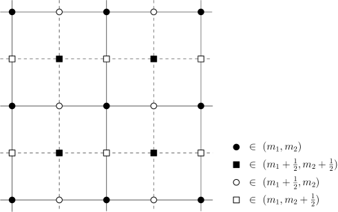
In this paper, mainly because of the advantages in dealing with the superfield formulation, we shall take the symmetric choice which is depicted in Fig. 1,

$$a = (+\frac{1}{2},+\frac{1}{2}),\hskip 10.0pta_{1}\ =\ (+\frac{1}{2},-\frac{1}{2}),\hskip 10.0pta_{2}\ =\ (-\frac{1}{2},+\frac{1}{2}),\hskip 10.0pt\tilde{a}\ =\ (-\frac{1}{2},-\frac{1}{2}).$$ (3.12)

Fig. 1: Symmetric choice of $a_{A}$

Superspace expressions for the supercharges $Q_{A}=(Q,Q_{\mu},\tilde{Q})$ which satisfy (3.8) are given by,

$$Q = \frac{\partial}{\partial\theta}+\frac{i}{2}\theta_{\mu}d^{+}_{\mu},\hskip 30.0ptQ_{\mu}\ =\ \frac{\partial}{\partial\theta_{\mu}}+\frac{i}{2}\theta d^{+}_{\mu}-\frac{i}{2}\tilde{\theta}\epsilon_{\mu\nu}d^{-}_{\nu},$$ (3.13)

$$\tilde{Q} = \frac{\partial}{\partial\tilde{\theta}}-\frac{i}{2}\theta_{\mu}\epsilon_{\mu\nu}d^{-}_{\nu}.$$ (3.14)

We also introduce the following supercovariant derivatives $D_{A}=(D,D_{\mu},\tilde{D})$,

$$D = \frac{\partial}{\partial\theta}-\frac{i}{2}\theta_{\mu}d^{+}_{\mu},\hskip 30.0ptD_{\mu}\ =\ \frac{\partial}{\partial\theta_{\mu}}-\frac{i}{2}\theta d^{+}_{\mu}+\frac{i}{2}\tilde{\theta}\epsilon_{\mu\nu}d^{-}_{\nu},$$ (3.15)

$$\tilde{D} = \frac{\partial}{\partial\tilde{\theta}}+\frac{i}{2}\theta_{\mu}\epsilon_{\mu\nu}d^{-}_{\nu},$$ (3.16)

which anti-commute with the supercharges, $\{Q_{A},D_{B}\}=0$, and satisfy the algebra,

$$\{D,D_{\mu}\} = -id^{+}_{\mu},\hskip 30.0pt\{\tilde{D},D_{\mu}\}\ =\ i\epsilon_{\mu\nu}d^{-}_{\nu},\hskip 30.0pt\{others\}\ =\ 0.$$ (3.17)

A chiral superfield $\Phi(x,\theta_{A},\overline{\theta}_{A})$ and an anti-chiral superfield $\overline{\Phi}(x,\theta_{A},\overline{\theta}_{A})$ on the lattice can be defined in terms of the supercovariant derivatives (3.15)-(3.16),

$$[\xi D,\Phi(x,\theta_{A},\overline{\theta}_{A})]_{*} = [\tilde{\xi}\tilde{D},\Phi(x,\theta_{A},\overline{\theta}_{A})]_{*}\ =\ 0,$$ (3.18)

$$[\xi_{\mu}D_{\mu},\overline{\Phi}(x,\theta_{A},\overline{\theta}_{A})]_{*} = 0\hskip 20.0pt\mathrm{(\mu\ :\ no\ sum)},$$ (3.19)

here and in the following we shall represent the arguments of the superfields by $\theta_{A}\equiv\theta_{\mu}=(\theta_{1},\theta_{2})$ and $\overline{\theta}_{A}\equiv(\theta,\tilde{\theta})$. In solving these conditions, it is convenient to introduce the following difference expansion operator,

$$U\equiv e^{-\frac{i}{2}(\theta\theta_{\mu}d^{+}_{\mu}-\epsilon_{\mu\nu}\tilde{\theta}\theta_{\mu}d^{-}_{\nu})}_{*},$$ (3.20)

where the exponential with the star is defined by

$$e^{X}_{*} \equiv 1+X+\frac{1}{2}X*X+\frac{1}{3!}X*X*X+\cdots.$$ (3.21)

The supercovariant derivatives (3.15-3.16) can be expressed in terms of $U$ as,

$$\xi D = U^{-1}*\xi\frac{\partial}{\partial\theta}*U,\hskip 20.0pt\tilde{\xi}\tilde{D}\ =\ U^{-1}*\tilde{\xi}\frac{\partial}{\partial\tilde{\theta}}*U,$$ (3.22)

$$\xi_{\mu}D_{\mu} = U*\xi_{\mu}\frac{\partial}{\partial\theta_{\mu}}*U^{-1}\hskip 20.0pt(\mathrm{\mu:\ no\ sum}),$$ (3.23)

with which one may rewrite the chiral and anti-chiral conditions (3.18)-(3.19) as

$$[\xi\frac{\partial}{\partial\theta},\Phi^{\prime}(x,\theta_{A},\overline{\theta}_{A})]_{*} = [\tilde{\xi}\frac{\partial}{\partial\tilde{\theta}},\Phi^{\prime}(x,\theta_{A},\overline{\theta}_{A})]_{*}\ =\ 0,$$ (3.24)

$$[\xi_{\mu}\frac{\partial}{\partial\theta_{\mu}},\overline{\Phi}^{\prime}(x,\theta_{A},\overline{\theta}_{A})]_{*} = 0\hskip 20.0pt\mathrm{(\mu\ :\ no\ sum)},$$ (3.25)

where $\Phi^{\prime}(x,\theta_{A},\overline{\theta}_{A})$ and $\overline{\Phi}^{\prime}(x,\theta_{A},\overline{\theta}_{A})$ are defined by

$$\Phi^{\prime}(x,\theta_{A},\overline{\theta}_{A}) = U*\Phi(x,\theta_{A},\overline{\theta}_{A})*U^{-1},\hskip 10.0pt\overline{\Phi}^{\prime}(x,\theta_{A},\overline{\theta}_{A})\ =\ U^{-1}*\overline{\Phi}(x,\theta_{A},\overline{\theta}_{A})*U.\qquad$$ (3.26)

One can easily solve the conditions (3.24) and (3.25) and get the following expressions for $\Phi^{\prime}$ and $\overline{\Phi}^{\prime}$,

$$\Phi^{\prime}(x,\theta_{A},\overline{\theta}_{A}) = \Phi^{\prime}(x,\theta_{A})\ =\ \phi(x)+\theta_{\mu}\psi_{\mu}(x)+\theta_{1}\theta_{2}\tilde{\phi}(x),$$ (3.27)

$$\overline{\Phi}^{\prime}(x,\theta_{A},\overline{\theta}_{A}) = \overline{\Phi}^{\prime}(x,\overline{\theta}_{A})\ =\ \varphi(x)+\theta\chi(x)+\tilde{\theta}\tilde{\chi}(x)+\theta\tilde{\theta}\tilde{\varphi}(x),$$ (3.28)

where $(\phi,\tilde{\phi},\varphi,\tilde{\varphi})$ and $(\psi_{1},\psi_{2},\chi,\tilde{\chi})$ are denoting the bosonic and fermionic component fields, respectively. Then the expressions of the chiral and anti-chiral superfields $(\Phi,\overline{\Phi})$ can be found as,

$$\Phi(x,\theta_{A},\overline{\theta}_{A}) = U^{-1}*\Phi^{\prime}(x,\theta_{A})*U$$ (3.29)

$$= \phi(x)+\theta_{\mu}\psi_{\mu}(x)+\theta_{1}\theta_{2}\tilde{\phi}(x)+\frac{i}{2}\theta\theta_{\mu}\Delta_{\mu}\phi(x)-\frac{i}{2}\epsilon_{\mu\nu}\tilde{\theta}\theta_{\mu}\Delta_{\nu}\phi(x)$$

$$+\frac{i}{2}\epsilon_{\mu\nu}\theta\theta_{1}\theta_{2}\Delta_{\mu}\psi_{\nu}(x)-\frac{i}{2}\tilde{\theta}\theta_{1}\theta_{2}\Delta_{\mu}\psi_{\mu}(x)+\frac{1}{4}\theta\tilde{\theta}\theta_{1}\theta_{2}\Delta_{\mu}\Delta_{\mu}\phi(x),$$

$$\overline{\Phi}(x,\theta_{A},\overline{\theta}_{A}) = U*\overline{\Phi}^{\prime}(x,\overline{\theta}_{A})*U^{-1}$$ (3.30)

$$= \varphi(x)+\theta\chi(x)+\tilde{\theta}\tilde{\chi}(x)+\theta\tilde{\theta}\tilde{\varphi}(x)-\frac{i}{2}\theta\theta_{\mu}\Delta_{\mu}\varphi(x)+\frac{i}{2}\epsilon_{\mu\nu}\tilde{\theta}\theta_{\mu}\Delta_{\nu}\varphi(x)$$

$$+\frac{i}{2}\epsilon_{\mu\nu}\theta\tilde{\theta}\theta_{\mu}\Delta_{\nu}\chi(x)+\frac{i}{2}\theta\tilde{\theta}\theta_{\mu}\Delta_{\mu}\tilde{\chi}(x)+\frac{1}{4}\theta\tilde{\theta}\theta_{1}\theta_{2}\Delta_{\mu}\Delta_{\mu}\varphi(x),$$

where $\Delta_{\mu}$ is denoting a symmetric difference operator, $\Delta_{\mu}f(x)=\frac{1}{2}(f(x+n_{\mu})-f(x-n_{\mu}))$. In deriving these expressions we made use of a star product version of the exponential formula,

$$e^{X}_{*}*Y*e^{-X}_{*} = Y+[X,Y]_{*}+\frac{1}{2!}[X,[X,Y]_{*}]_{*}+\cdots,$$ (3.31)

which obeys from the associativity of the star product.

The $\mathcal{N}=D=2$ twisted SUSY transformation laws for the component fields follow from the definition (2.21). As for the chiral superfield $\Phi(x,\theta_{A},\overline{\theta}_{A})$, we have

$$\delta_{\xi_{A}}\Phi(x,\theta_{B},\overline{\theta}_{B}) = U^{-1}*\delta_{\xi_{A}}\Phi^{\prime}(x,\theta_{B})*U$$ (3.32)

$$= [\xi_{A}Q_{A},U^{-1}*\Phi^{\prime}(x,\theta_{B})*U]_{*},$$

from which it obeys

$$\delta_{\xi_{A}}\Phi^{\prime}(x,\theta_{B}) = [\xi_{A}Q^{\prime}_{A},\Phi^{\prime}(x,\theta_{B})]_{*},$$ (3.33)

where $\xi_{A}Q^{\prime}_{A}\equiv U*\xi_{A}Q_{A}*U^{-1}$ are given by

$$\xi Q^{\prime} = \xi\frac{\partial}{\partial\theta}+i\xi\theta_{\mu}d^{+}_{\mu},\hskip 20.0pt\xi_{\mu}Q^{\prime}_{\mu}\ =\ \xi_{\mu}\frac{\partial}{\partial\theta_{\mu}}\ \ \ \ (\mu:\mathrm{no\ sum}),$$ (3.34)

$$\tilde{\xi}\tilde{Q}^{\prime} = \tilde{\xi}\frac{\partial}{\partial\tilde{\theta}}-i\tilde{\xi}\theta_{\mu}\epsilon_{\mu\nu}d^{-}_{\nu}.$$ (3.35)

In a similar way for the anti-chiral superfield $\overline{\Phi}(x,\theta_{A},\overline{\theta}_{A})$, we have

$$\delta_{\xi_{A}}\overline{\Phi}^{\prime}(x,\overline{\theta}_{A}) = [\xi_{A}Q^{\prime\prime}_{A},\overline{\Phi}^{\prime}(x,\overline{\theta}_{A})]_{*},$$ (3.36)

where $\xi_{A}Q^{\prime\prime}_{A}\equiv U^{-1}*\xi_{A}Q_{A}*U$ are given by

$$\xi Q^{\prime\prime} = \xi\frac{\partial}{\partial\theta},\hskip 20.0pt\xi_{\mu}Q^{\prime\prime}_{\mu}\ =\ \xi_{\mu}\frac{\partial}{\partial\theta_{\mu}}+i\xi_{\mu}\theta d^{+}_{\mu}-i\xi_{\mu}\tilde{\theta}\epsilon_{\mu\nu}d^{-}_{\nu}\ \ \ \ (\mu:\mathrm{no\ sum}),$$ (3.37)

$$\tilde{\xi}\tilde{Q}^{\prime\prime} = \tilde{\xi}\frac{\partial}{\partial\tilde{\theta}}.$$ (3.38)

The $\mathcal{N}=D=2$ twisted SUSY transformation laws for the component fields are summarized in Table 1. One can verify that the component-wise SUSY variations form the following off-shell closed algebra,

$$[\delta_{\xi},\delta_{\xi_{\rho}}]\varphi_{A} = +i\xi\xi_{\rho}\Delta_{\rho}\varphi_{A}\hskip 20.0pt(\mathrm{\rho:no\ sum}),$$ (3.39)

$$[\delta_{\tilde{\xi}},\delta_{\xi_{\rho}}]\varphi_{A} = -i\tilde{\xi}\xi_{\rho}\epsilon_{\rho\sigma}\Delta_{\sigma}\varphi_{A}\hskip 20.0pt(\mathrm{\rho:no\ sum}),$$ (3.40)

$$[others]\varphi_{A} = 0,$$ (3.41)

where $\varphi_{A}$ denotes any of the component field $(\phi,\psi_{\mu},\tilde{\phi},\varphi,\chi,\tilde{\chi},\tilde{\varphi})$.

	$\delta_{\xi}$	$\delta_{\xi_{\rho}}$	$\delta_{\tilde{\xi}}$
$\phi(x)$	$0$	$\xi_{\rho}\psi_{\rho}(x)$	$0$
$\psi_{\mu}(x)$	$-i\xi\Delta_{\mu}\phi(x)$	$\epsilon_{\mu\rho}\xi_{\rho}\tilde{\phi}(x)$	$i\epsilon_{\mu\rho}\tilde{\xi}\Delta_{\rho}\phi(x)$
$\tilde{\phi}(x)$	$i\xi\epsilon_{\rho\sigma}\Delta_{\rho}\psi_{\sigma}(x)$	$0$	$-i\tilde{\xi}\Delta_{\rho}\psi_{\rho}(x)$
$\varphi(x)$	$\xi\chi(x)$	$0$	$\tilde{\xi}\tilde{\chi}(x)$
$\chi(x)$	$0$	$-i\xi_{\rho}\Delta_{\rho}\varphi(x)$	$\tilde{\xi}\tilde{\varphi}(x)$
$\tilde{\chi}(x)$	$-\xi\tilde{\varphi}(x)$	$i\epsilon_{\rho\sigma}\xi_{\rho}\Delta_{\sigma}\varphi(x)$	$0$
$\tilde{\varphi}(x)$	$0$	$i\xi_{\rho}\Delta_{\rho}\tilde{\chi}(x)+i\xi_{\rho}\epsilon_{\rho\sigma}\Delta_{\sigma}\chi(x)$	$0$

Table 1: $\mathcal{N}=D=2$ twisted SUSY transformation laws on the lattice for the component fields $(\phi,\psi_{\mu},\tilde{\phi})$ and $(\varphi,\chi,\tilde{\chi},\tilde{\varphi})$.

3.2 Twisted SUSY invariant action at tree level

In terms of the chiral and anti-chiral superfields $\Phi(x,\theta_{A})$ and $\overline{\Phi}(x,\theta_{A})$, one can generally construct a $\mathcal{N}=D=2$ twisted SUSY invariant action on the lattice as

$$S = \sum_{x}\int d^{4}\theta\ K_{*}(\overline{\Phi},\Phi)+\sum_{x}\int d^{2}\theta\ F_{*}(\Phi)+\sum_{x}\int d^{2}\overline{\theta}\ \overline{F}_{*}(\overline{\Phi})$$ (3.42)

where the Grassmann measures are defined by $d^{4}\theta\equiv d\theta d\tilde{\theta}d\theta_{1}d\theta_{2}$, $d^{2}\theta\equiv d\theta_{2}d\theta_{1}$ and $d^{2}\overline{\theta}\equiv d\tilde{\theta}d\theta$, and each Grassmann integration is defined by $\int d\theta_{A}\ 1=0$, $\int d\theta_{A}\theta_{B}=\delta_{AB}$. The symbol $K_{*}$ is denoting any functions of the chiral and anti-chiral superfields in terms of the star product, while the symbols $F_{*}$ and $\overline{F}_{*}$ are respectively denoting any functions of the chiral superfields and anti-chiral superfields again in terms of the star product. Since we take the symmetric choice of $a_{A}$ (3.12), the summation over $x$ should cover (int, int) sites as well as (half-int, half-int) sites,

$$\sum_{x} = \sum_{(m_{1},m_{2})}+\sum_{(m_{1}+\frac{1}{2},m_{2}+\frac{1}{2})}\hskip 20.0pt(m_{1},m_{2}:\mathrm{integers}).$$ (3.43)

The necessity of summing over both (int,int) sites and (half-int,half-int) sites stems from the fact that in the symmetric choice of $a_{A}$ the lattice SUSY transformation can essentially be regarded as a mapping from (int,int) to (half-int,half-int) or vice versa, due to the non-commutativity associated with $\theta_{A}$ and $\xi_{A}$. The simplest action with mass and interaction terms can be given by a $\mathcal{N}=D=2$ Dirac-Kähler twisted analog of the Wess-Zumino model [18],

$$K_{*}=\overline{\Phi}*\Phi,\hskip 20.0ptF_{*}=\frac{m}{2}\Phi*\Phi+\frac{g}{3!}\Phi*\Phi*\Phi,\hskip 20.0pt\overline{F}_{*}=\frac{m}{2}\overline{\Phi}*\overline{\Phi}+\frac{g}{3!}\overline{\Phi}*\overline{\Phi}*\overline{\Phi}.$$ (3.44)

The total action $S_{WZ}$ is accordingly given by,

$$S_{WZ} = S_{kin}+S_{mass}+S_{int},$$ (3.45)

where the kinetic terms $S_{kin}$, the mass terms $S_{mass}$ and the interaction terms $S_{int}$ are expressed in terms of the component fields as,

$$S_{kin} = \sum_{x}\int d^{4}\theta\ \overline{\Phi}(x,\theta_{A},\overline{\theta}_{A})*\Phi(x,\theta_{A},\overline{\theta}_{A})$$ (3.46)

$$= \sum_{x}\biggl{[}\varphi(x)\Delta_{\mu}\Delta_{\mu}\phi(x)+i\chi(x)\Delta_{\mu}\psi_{\mu}(x)+i\epsilon_{\mu\nu}\tilde{\chi}(x)\Delta_{\mu}\psi_{\nu}(x)+\tilde{\varphi}(x)\tilde{\phi}(x)\biggr{]},\qquad$$

$$S_{mass} = \frac{m}{2}\sum_{x}\biggl{[}\int d^{2}\theta\ \Phi(x,\theta_{A},\overline{\theta}_{A})*\Phi(x,\theta_{A},\overline{\theta}_{A})+\int d^{2}\overline{\theta}\ \overline{\Phi}(x,\theta_{A},\overline{\theta}_{A})*\overline{\Phi}(x,\theta_{A},\overline{\theta}_{A})\biggr{]}$$ (3.47)

$$= \frac{m}{2}\sum_{x}\biggl{[}\phi(x)\tilde{\phi}(x)+\tilde{\phi}(x)\phi(x)-\epsilon_{\mu\nu}\psi_{\mu}(x)\psi_{\nu}(x)$$

$$+\varphi(x)\tilde{\varphi}(x)+\tilde{\varphi}(x)\varphi(x)-\chi(x)\tilde{\chi}(x)+\tilde{\chi}(x)\chi(x)\biggr{]},$$

$$S_{int} = \frac{g}{3!}\sum_{x}\biggl{[}\int d^{2}\theta\ \Phi(x,\theta_{A},\overline{\theta}_{A})*\Phi(x,\theta_{A},\overline{\theta}_{A})*\Phi(x,\theta_{A},\overline{\theta}_{A})$$ (3.48)

$$+\int d^{2}\overline{\theta}\ \overline{\Phi}(x,\theta_{A},\overline{\theta}_{A})*\overline{\Phi}(x,\theta_{A},\overline{\theta}_{A})*\overline{\Phi}(x,\theta_{A},\overline{\theta}_{A})\biggr{]}$$

$$= \frac{g}{3!}\sum_{x}\biggl{[}-\epsilon_{\mu\nu}\phi(x)\psi_{\mu}(x+a_{\nu})\psi_{\nu}(x-a_{\mu})-\epsilon_{\mu\nu}\psi_{\mu}(x+a_{\nu})\psi_{\nu}(x-a_{\mu})\phi(x)$$

$$-\epsilon_{\mu\nu}\psi_{\mu}(x-a_{\nu})\phi(x)\psi_{\nu}(x+a_{\mu})+\phi(x)\phi(x)\tilde{\phi}(x)+\phi(x)\tilde{\phi}(x)\phi(x)+\tilde{\phi}(x)\phi(x)\phi(x)$$

$$-\varphi(x)\chi(x+\tilde{a})\tilde{\chi}(x-a)+\varphi(x)\tilde{\chi}(x+a)\chi(x-\tilde{a})-\chi(x+\tilde{a})\tilde{\chi}(x-a)\varphi(x)$$

$$+\tilde{\chi}(x+a)\chi(x-\tilde{a})\varphi(x)-\chi(x-\tilde{a})\varphi(x)\tilde{\chi}(x+a)+\tilde{\chi}(x-a)\varphi(x)\chi(x+\tilde{a})$$

$$+\varphi(x)\varphi(x)\tilde{\varphi}(x)+\varphi(x)\tilde{\varphi}(x)\varphi(x)+\tilde{\varphi}(x)\varphi(x)\varphi(x)\biggr{]},$$

where we used the symmetric nature of the shift parameters (3.12), $a_{1}+a_{2}=0$, $a+\tilde{a}=0$. One should notice that the kinetic terms (3.46) and mass terms (3.47) consist of the component fields living only on (int, int) sites or (half-int, half-int) sites, which implies that the field propagations are restricted only from (int, int) to (int, int) or from (half-int, half-int) to (half-int, half-int) sites. On the other hand, the interaction terms (3.48) involve both (int, int) and (half-int, half-int) sites. In particular, the Yukawa coupling terms consist of the bosonic field at an (int, int) site and the fermionic fields at (half-int, half-int) sites or vice versa.

The twisted $\mathcal{N}=D=2$ SUSY invariant nature of the total action is manifest from their superfield expressions, since the star products of the superfields satisfy the Leibniz rule (2.27) which is also valid for a product of three superfields,

$$\delta_{A}(\Phi_{1}*\Phi_{2}*\Phi_{3}) = \delta_{A}\Phi_{1}*\Phi_{2}*\Phi_{3}+\Phi_{1}*\delta_{A}\Phi_{2}*\Phi_{3}+\Phi_{1}*\Phi_{2}*\delta_{A}\Phi_{3}.$$ (3.49)

It is important to note that the above star product nature is implicitly inherited also in the component-wise expressions. Actually, in order to be consistent with the star product nature of the superfields which preserves the Leibniz rule, one needs to recognize that the SUSY variation of each component field should be associated with the star product, for example,

$$\delta_{A}(\phi(x)\phi(x)\tilde{\phi}(x)) = \delta_{A}\phi(x)*\phi(x)\tilde{\phi}(x)+\phi(x)*\delta_{A}\phi(x)*\tilde{\phi}(x)+\phi(x)\phi(x)*\delta_{A}\tilde{\phi}(x).$$

Since the component-wise SUSY variations are defined together with the Grassmann parameter $\xi_{A}$’s, one needs to take care about the ordering of the component fields in showing the SUSY invariance, even though each component field is defined as an ordinary bosonic or fermionic function. For instance,

$$\delta_{A}(\phi(x)\tilde{\phi}(x))\neq\delta_{A}(\tilde{\phi}(x)\phi(x)),$$ (3.51)

even though we have $\phi(x)\tilde{\phi}(x)=\tilde{\phi}(x)\phi(x)$. These properties of the lattice SUSY transformation laws essentially necessitates the notion of “proper” ordering in the component-wise expressions. For this reason, we respected the orderings of the component fields in the expressions (3.46)-(3.48). It is a straightforward task to verify that these proper ordered component-wise expressions for the action (3.46)-(3.48) are manifestly invariant under all the $\mathcal{N}=D=2$ twisted SUSY transformations on the lattice.

We note here that the notion of “proper” ordering in the component-wise expression has been already argued in Ref. [3, 6] in replying to the critiques claimed in Ref [5], and now we are revisiting this issue again with the star product formulation at hand. It is obvious that the necessity of “proper” ordering stems from the intrinsic non-commutative nature of the star product defined in (2.8) and is ultimately originated from the nature of the Leibniz rule for the difference operations. Now the question is how this kind of “proper” ordering can be survived or respected in the quantum treatment of the formulation. This is actually the main subject of this paper. We anticipate the result and claim here that respecting the “proper” ordering essentially corresponds to picking up the planar diagrams in the perturbative expansions. Developing the superfield formulation, we will explicitly see in Sec. 5 that in the planar diagrams all the phase factors which stem from the non-commutativity strictly protect the SUSY structure on the lattice and give the exact SUSY result. In other words, the above notion of “proper” ordering can be preserved and respected in the planar limit or in the ‘t Hooft large-$N$ limit. Thus, the exact SUSY w.r.t. all the supercharges at non-zero lattice spacing is achieved in this limit.

We also note some important properties of superfield integrations under the $x$-summation (3.43). For the kinetic term or the D-term, we have,

$$\sum_{x}\int d^{4}\theta\ \overline{\Phi}*\Phi = \sum_{x}\int d^{4}\theta\ \overline{\Phi}\Phi\ =\ \sum_{x}\int d^{4}\theta\ \Phi\overline{\Phi},$$ (3.52)

which stems from the vanishing sum of the shift parameters (3.11). For the F-terms in particular for the mass terms, we have,

$$\sum_{x}\int d^{2}\theta\ \Phi_{1}*\Phi_{2} = \sum_{x}\int d^{2}\theta\ \Phi_{1}\Phi_{2}\ =\ \sum_{x}\int d^{2}\theta\ \Phi_{2}\Phi_{1},$$ (3.53)

$$\sum_{x}\int d^{2}\overline{\theta}\ \overline{\Phi}_{1}*\overline{\Phi}_{2} = \sum_{x}\int d^{2}\overline{\theta}\ \overline{\Phi}_{1}\overline{\Phi}_{2}\ =\ \sum_{x}\int d^{2}\overline{\theta}\ \overline{\Phi}_{2}\overline{\Phi}_{1},$$ (3.54)

thanks to the symmetric choice of the shift parameter (3.12). Namely, the kinetic and mass terms can be written without the star product under the $x$-summation (3.43). This is a preferable feature for the superfield formulation, particularly in deriving the superfield propagators as we will see in the next subsection. For the interaction terms, we have the cyclic permutation property for the (anti-)chiral superfields,

$$\sum_{x}\int d^{2}\theta\ \Phi_{1}*\Phi_{2}*\Phi_{3} = \sum_{x}\int d^{2}\theta\ \Phi_{2}*\Phi_{3}*\Phi_{1}\ =\ \sum_{x}\int d^{2}\theta\ \Phi_{3}*\Phi_{1}*\Phi_{2},$$ (3.55)

$$\sum_{x}\int d^{2}\overline{\theta}\ \overline{\Phi}_{1}*\overline{\Phi}_{2}*\overline{\Phi}_{3} = \sum_{x}\int d^{2}\overline{\theta}\ \overline{\Phi}_{2}*\overline{\Phi}_{3}*\overline{\Phi}_{1}\ =\ \sum_{x}\int d^{2}\overline{\theta}\ \overline{\Phi}_{3}*\overline{\Phi}_{1}*\overline{\Phi}_{2},$$ (3.56)

which is again thanks to the symmetric choice (3.12). Actually, one can show that the equalities in (3.53) and (3.55) hold only if one takes $a_{1}+a_{2}=0$. Likewise, the equalities in (3.54) and (3.56) hold only if one takes $a+\tilde{a}=0$. This technical advantage is the main reason why we take the symmetric choice (3.12).

Although the summation defined in (3.43) is already sufficient for ensuring the SUSY invariant nature of the total action, in the following for the technical convenience in the momentum analysis, we will conventionally take the $x$-summation to cover (int, half-int) and (half-int,int) sites as well,

$$\sum_{x} = \sum_{(m_{1},m_{2})}+\sum_{(m_{1}+\frac{1}{2},m_{2}+\frac{1}{2})}+\sum_{(m_{1}+\frac{1}{2},m_{2})}+\sum_{(m_{1},m_{2}+\frac{1}{2})},\hskip 10.0pt(m_{1},m_{2}\ :\mathrm{integers}).$$ (3.57)

Namely, we consider a finer lattice which can be measured by half of the unit length. Accordingly, the field propagations are now also allowed from (int, half-int) to (int, half-int) and (half-int, int) to (half-int, int) sites. Notice that the lattice action defined by the $x$-summation over (int,int) and (half-int,half-int) is totally independent from the one given by (half-int,int) and (int,half-int) in the sense that they are not correlated each other neither dynamically nor supersymmetrically. The multiplicity of the superfields introduced so far is summarized as follows. The SUSY invariance essentially requires the (super)fields defined on both (int,int) and (half-int, half-int) sites as in (3.43). This causes the field multiplicity of factor 2. Furthermore, as explained above, we conventionally introduced a trivial multiplicity of factor 2 which stems from the summation (3.57). The entire multiplicity of the superfields originated from the $x$-summation is then

$$2(\mathrm{SUSY})\times 2(\mathrm{conventional})=4.$$ (3.58)

We observe that the lattice action subject to the $x$-summation given in (3.57) describes four copies of the $D=\mathcal{N}=2$ twisted Wess-Zumino model in the naive continuum limit. We will come back this point when dealing with the momentum space analysis of the superfield propagators in the next section. The lattice superfield configuration subject to the $x$-summation (3.57) is depicted in Fig. 2.

Fig. 2: Configuration of the superfields in the action subject to the $x$-summation (3.57)

3.3 Superfield propagators

Having defined the $\mathcal{N}=D=2$ twisted SUSY invariant action on the lattice, we shall proceed to set up the technical ingredients requisite for studying the possible quantum corrections. We shall take a full advantage of the lattice superfield method and intend to calculate the radiative corrections entirely in the superfield method. In what follows we derive the superfield propagators on the lattice. The notion of superfield propagators was first introduced in [14, 15]. The derivation in this section basically follows the same procedure as in the continuum spacetime [15, 17] or in the Moyal non-commutative spacetime [19]. We start from the free part of the tree level vertex functional, which we shall denote as $\Gamma_{0}$. It is given by the free part of the lattice action (3.45). Using the relations (3.26), we express it in terms of $\Phi^{\prime}$ and $\overline{\Phi}^{\prime}$ in (3.27)-(3.28),

$$\Gamma_{0}[\Phi,\overline{\Phi}] = \sum_{x}\int d^{4}\theta\ (U^{2}*\overline{\Phi}^{\prime}*U^{-2})\Phi^{\prime}+\frac{m}{2}\sum_{x}\biggl{[}\int d^{2}\theta\ \Phi^{\prime}\Phi^{\prime}+\int d^{2}\overline{\theta}\ \overline{\Phi}^{\prime}\overline{\Phi}^{\prime}\biggr{]}$$ (3.59)

$$= \sum_{x}\int d^{4}\theta\ \overline{\Phi}^{\prime}(U^{-2}*\Phi^{\prime}*U^{2})+\frac{m}{2}\sum_{x}\biggl{[}\int d^{2}\theta\ \Phi^{\prime}\Phi^{\prime}+\int d^{2}\overline{\theta}\ \overline{\Phi}^{\prime}\overline{\Phi}^{\prime}\biggr{]},$$ (3.60)

where the $U$ is denoting the difference expansion operator defined in (3.20), and the Grassmann integration measures are again defined by $d^{4}\theta\equiv d\theta d\tilde{\theta}d\theta_{1}d\theta_{2}$, $d^{2}\theta\equiv d\theta_{2}d\theta_{1}$ and $d^{2}\overline{\theta}\equiv d\tilde{\theta}d\theta$. The corresponding connected Green’s functional, which we denote as $W_{0}$, is defined by the Legendre transformation,

$$W_{0}[J,\overline{J}] = \Gamma_{0}[\Phi,\overline{\Phi}]+\sum_{x}\biggl{[}\int d^{2}\theta\ J^{\prime}\Phi^{\prime}+\int d^{2}\overline{\theta}\ \overline{J}^{\prime}\overline{\Phi}^{\prime}\biggr{]},$$ (3.61)

where $J^{\prime}$ and $\overline{J}^{\prime}$ denote the chiral and anti-chiral source superfields which obey the same conditions as $\Phi^{\prime}$ (3.24) and $\overline{\Phi}^{\prime}$ (3.25), respectively,

$$[\xi\frac{\partial}{\partial\theta},J^{\prime}(x,\theta_{A})]_{*} = [\tilde{\xi}\frac{\partial}{\partial\tilde{\theta}},J^{\prime}(x,\theta_{A})]_{*}\ =\ 0,$$ (3.62)

$$[\xi_{\mu}\frac{\partial}{\partial\theta_{\mu}},\overline{J}^{\prime}(x,\overline{\theta}_{A})]_{*} = 0,\hskip 20.0pt(\mathrm{\mu\ :\ no\ sum}).$$ (3.63)

The Legendre transformation (3.61) gives rise to the relations between $(J^{\prime},\overline{J}^{\prime})$ and $(\Phi^{\prime},\overline{\Phi}^{\prime})$,

$$\frac{\delta\Gamma_{0}}{\delta\Phi^{\prime}} = -J^{\prime},\hskip 20.0pt\frac{\delta\Gamma_{0}}{\delta\overline{\Phi}^{\prime}}\ =\ -\overline{J}^{\prime},$$ (3.64)

$$\frac{\delta W_{0}}{\delta J^{\prime}} = \Phi^{\prime},\hskip 25.0pt\frac{\delta W_{0}}{\delta\overline{J}^{\prime}}\ =\ \overline{\Phi}^{\prime}.$$ (3.65)

The superfield propagators for $\Phi^{\prime}$ and $\overline{\Phi}^{\prime}$ are defined in terms of the functional derivatives of the connected Green’s functional w.r.t. the source superfields $(J^{\prime},\overline{J}^{\prime})$,

$$<\Phi^{\prime}(1)\Phi^{\prime}(2)> \equiv \frac{\delta^{2}}{\delta J^{\prime}(1)\delta J^{\prime}(2)}W_{0}[J,\overline{J}]\ =\ \frac{\delta}{\delta J^{\prime}(1)}\Phi^{\prime}[J,\overline{J}](2),$$ (3.66)

$$<\overline{\Phi}^{\prime}(1)\Phi^{\prime}(2)> \equiv \frac{\delta^{2}}{\delta\overline{J}^{\prime}(1)\delta J^{\prime}(2)}W_{0}[J,\overline{J}]\ =\ \frac{\delta}{\delta\overline{J}^{\prime}(1)}\Phi^{\prime}[J,\overline{J}](2),$$ (3.67)

where the arguments 1 and 2 refer to each superspace point. In the second equalities, we used the relations (3.65).

In order to calculate the superfield propagators, we first need to write down the l.h.s.’s of the relations (3.64) explicitly, and then solve them w.r.t. $\Phi^{\prime}$ and $\overline{\Phi}^{\prime}$. By functionally differentiating the expressions (3.59) and (3.60) by $\Phi^{\prime}$ and $\overline{\Phi}^{\prime}$, respectively, we actually have,

$$\int d^{2}\overline{\theta}^{(1)}\ U^{2}(1)*\overline{\Phi}^{\prime}(1)*U^{-2}(1)+m\Phi^{\prime}(1) = -J^{\prime}(1),$$ (3.68)

$$\int d^{2}\theta^{(1)}\ U^{-2}(1)*\Phi^{\prime}(1)*U^{2}(1)+m\Phi^{\prime}(1) = -\overline{J}^{\prime}(1).$$ (3.69)

In deriving them, we made use of the functional differential relations for $(\Phi^{\prime},\overline{\Phi}^{\prime})$,

$$\frac{\delta\Phi^{\prime}(2)}{\delta\Phi^{\prime}(1)} = \delta^{2}_{x^{(1)},x^{(2)}}\delta^{2}(\theta^{(1)}-\theta^{(2)}),\hskip 20.0pt\frac{\delta\overline{\Phi}^{\prime}(2)}{\delta\overline{\Phi}^{\prime}(1)}\ =\ \delta^{2}_{x^{(1)},x^{(2)}}\delta^{2}(\overline{\theta}^{(1)}-\overline{\theta}^{(2)}),$$ (3.70)

where $\delta^{2}_{x^{(1)},x^{(2)}}$ denotes the two dimensional Kronecker delta, while the delta functions for the Grassmann coordinates $\delta^{2}(\theta^{(1)}-\theta^{(2)})$ and $\delta^{2}(\overline{\theta}^{(1)}-\overline{\theta}^{(2)})$ are defined by

$$\delta^{2}(\theta^{(1)}-\theta^{(2)}) = \prod_{A}(\theta^{(1)}_{A}-\theta^{(2)}_{A})\ =\ (\theta^{(1)}_{1}-\theta^{(2)}_{1})(\theta^{(1)}_{2}-\theta^{(2)}_{2}),$$ (3.71)

$$\delta^{2}(\overline{\theta}^{(1)}-\overline{\theta}^{(2)}) = \prod_{A}(\overline{\theta}^{(1)}_{A}-\overline{\theta}^{(2)}_{A})\ =\ (\theta^{(1)}-\theta^{(2)})(\tilde{\theta}^{(1)}-\tilde{\theta}^{(2)}).$$ (3.72)

Operating $U^{2}\,*\,$ from the left and $\,*\,U^{-2}$ from the right on (3.69) and taking the $d^{2}\overline{\theta}$ integration would give

$$\Delta_{\mu}^{2}\Phi^{\prime}(1)+m\int d^{2}\overline{\theta}^{(1)}\ U^{2}(1)*\overline{\Phi}^{\prime}(1)*U^{-2}(1)=-\int d^{2}\overline{\theta}^{(1)}\ U^{2}(1)*\overline{J}^{\prime}(1)*U^{-2}(1),$$ (3.73)

and the similar expression for (3.68) by operating $U^{-2}\,*\,$ from the left and $\,*\,U^{2}$ from the right. In (3.73) we used the following relation which can be verified explicitly,

$$\int d^{2}\overline{\theta}\ U^{2}*\biggl{[}\int d^{2}\theta\ U^{-2}*\Phi^{\prime}(x,\theta_{A})*U^{2}\biggr{]}*U^{-2}=\Delta_{\mu}^{2}\Phi^{\prime}(x,\theta_{A}).$$ (3.74)

By substituting (3.68) into (3.73) and solving it w.r.t. $\Phi^{\prime}$ we then obtain

$$\Phi^{\prime}(1) = \frac{-1}{\Delta_{\mu}^{2}-m^{2}}\int d^{2}\overline{\theta}^{(1)}\ U^{2}(1)*\overline{J}^{\prime}(1)*U^{-2}(1)+\frac{m}{\Delta_{\mu}^{2}-m^{2}}J^{\prime}(1).$$ (3.75)

Likewise we obtain for $\overline{\Phi}^{\prime}$,

$$\overline{\Phi}^{\prime}(1) = \frac{-1}{\Delta_{\mu}^{2}-m^{2}}\int d^{2}\theta^{(1)}\ U^{-2}(1)*J^{\prime}(1)*U^{2}(1)+\frac{m}{\Delta_{\mu}^{2}-m^{2}}\overline{J}^{\prime}(1).$$ (3.76)

By functionally differentiating the relations (3.75)-(3.76) w.r.t. the source superfields $J^{\prime}$ and $\overline{J}^{\prime}$ and using the definitions (3.66)-(3.67), we finally obtain the superfield propagators which are given by

$$<\Phi^{\prime}(x^{(1)},\theta^{(1)}_{A})\Phi^{\prime}(x^{(2)},\theta^{(2)}_{A})> = \frac{m}{\Delta_{\mu}^{2}-m^{2}}\delta^{2}_{x^{(1)},x^{(2)}}\delta^{2}(\theta^{(1)}-\theta^{(2)})$$ (3.77)

$$= \int^{2\pi}_{-2\pi}\frac{d^{2}p}{(4\pi)^{2}}e^{ip(x^{(1)}-x^{(2)})}\frac{-m}{\sin^{2}{p_{\mu}}+m^{2}}\delta^{2}(\theta^{(1)}-\theta^{(2)}),\qquad$$

$$<\overline{\Phi}^{\prime}(x^{(1)},\overline{\theta}^{(1)}_{A})\overline{\Phi}^{\prime}(x^{(2)},\overline{\theta}^{(2)}_{A})> = \frac{m}{\Delta_{\mu}^{2}-m^{2}}\delta^{2}_{x^{(1)},x^{(2)}}\delta^{2}(\overline{\theta}^{(1)}-\overline{\theta}^{(2)})$$ (3.78)

$$= \int^{2\pi}_{-2\pi}\frac{d^{2}p}{(4\pi)^{2}}e^{ip(x^{(1)}-x^{(2)})}\frac{-m}{\sin^{2}{p_{\mu}}+m^{2}}\delta^{2}(\overline{\theta}^{(1)}-\overline{\theta}^{(2)}),$$

$$<\overline{\Phi}^{\prime}(x^{(1)},\overline{\theta}^{(1)}_{A})\Phi^{\prime}(x^{(2)},\theta^{(2)}_{A})> = \frac{-1}{\Delta_{\mu}^{2}-m^{2}}e^{+iE^{(12)}_{\mu}\Delta_{\mu}^{(1)}}\ \delta^{2}_{x^{(1)},x^{(2)}}$$ (3.79)

$$= \int^{2\pi}_{-2\pi}\frac{d^{2}p}{(4\pi)^{2}}e^{ip(x^{(1)}-x^{(2)})}\frac{e^{-E^{(12)}_{\mu}\sin{p_{\mu}}}}{\sin^{2}{p_{\mu}}+m^{2}},$$

$$<\Phi^{\prime}(x^{(1)},\theta^{(1)}_{A})\overline{\Phi}^{\prime}(x^{(2)},\overline{\theta}^{(2)}_{A})> = \frac{-1}{\Delta_{\mu}^{2}-m^{2}}e^{-iE^{(21)}_{\mu}\Delta_{\mu}^{(1)}}\ \delta^{2}_{x^{(1)},x^{(2)}}$$ (3.80)

$$= \int^{2\pi}_{-2\pi}\frac{d^{2}p}{(4\pi)^{2}}e^{ip(x^{(1)}-x^{(2)})}\frac{e^{+E^{(21)}_{\mu}\sin{p_{\mu}}}}{\sin^{2}{p_{\mu}}+m^{2}},$$

where the symbols $E^{(12)}$ and $E^{(21)}$ are defined by $E^{(ij)}_{\mu}\equiv\theta^{(i)}\theta_{\mu}^{(j)}+\epsilon_{\mu\nu}\tilde{\theta}^{(i)}\theta_{\nu}^{(j)}$ for $i,j=1\ \mathrm{or}\ 2$. In each second line of these expressions, we inserted the momentum space representation of $\delta^{2}_{x^{(1)},x^{(2)}}$,

$$\delta^{2}_{x^{(1)},x^{(2)}} = \int^{2\pi}_{-2\pi}\frac{d^{2}p}{(2\pi)^{2}}e^{ip(x^{(1)}-x^{(2)})}.$$ (3.81)

Notice that the the range of the Brillouin zone is $4\pi$ for each direction since we introduced the superfields located on the half-integer sites for each spacetime direction. Within that range of the Brillouin zone, each propagator (3.77)-(3.80) has superficially 16 spectrum doubling, namely, 4 species for each direction.

It is important to recognize that the entire doubling is originated from the two reasons. The first one is due to the $x$-summation over the half-integer sites (3.57). This can be regarded as a trivial multiplicity as far as the superfield propagators are concerned, since the field propagations are only restricted from (int,int) to (int,int), (int,half-int) to (int,half-int), (half-int,int) to (half-int,int) and (half-int,half-int) to (half-int,half-int) sites. In the configuration space, this is clear from the fact that each term in the kinetic action (3.46) consists of (int,int), (half-int,half-int), (int,half-int) or (half-int,int) sites. In the momentum space this feature is reflected to the $2\pi$ periodicity of the integrand in each propagator except for the exponential factor. In fact, starting from the above expressions of the propagators (3.77)-(3.80), one easily sees that there are no correlations between the integer and the half-integer sites for each direction. For instance, the propagator (3.77) can be re-expressed as

$$<\Phi^{\prime}(x^{(1)},\theta^{(1)}_{A})\Phi^{\prime}(x^{(2)},\theta^{(2)}_{A})>$$

$$\hskip 5.0pt=\biggl{\{}\begin{array}[]{l}\displaystyle\int^{\pi}_{-\pi}\frac{d^{2}p}{(2\pi)^{2}}e^{ip(x^{(1)}-x^{(2)})}\frac{-m}{\sin^{2}{p_{\mu}}+m^{2}}\delta^{2}(\theta^{(1)}-\theta^{(2)}),\ \ \mathrm{for}\ \ x^{(1)}-x^{(2)}=(m_{1},m_{2})\\ 0,\ \ \ \mathrm{otherwise}\end{array}$$ (3.84)

where $m_{1}$ and $m_{2}$ denote any integer values. Note that the range of the Brillouin zone for the non-vanishing propagator is now taken as $2\pi$ since the integrand is actually $2\pi$ periodic. In deriving this expression, we divided the momentum regions into two of $2\pi$ and made use of the $2\pi$ (anti-)periodicity of the exponential factor $e^{ip(x^{(1)}-x^{(2)})}$. The other propagators (3.79)-(3.80) also have the same feature. This observation implies that the factor $4$ in the entire multiplicity due to the $x$-summation over half-integer sites are just corresponding to the four copies of the physically equivalent momentum regions as long as the propagators are concerned.

In contrast, the rest of the spectrum doubling which still remains in the propagators has a non-trivial physical meaning via the $D=\mathcal{N}=2$ Dirac-Kähler mechanism. This stems from the fact that the chiral and anti-chiral superfields $(\Phi^{\prime},\overline{\Phi}^{\prime})$ contain the components of the Dirac-Kähler twisted fermions $(\chi,\psi_{\mu},\tilde{\chi})$ which turn into the corresponding staggered fermion components on the lattice. In this procedure, the extended $\mathcal{N}=2$ SUSY index can be regarded as $N_{f}=2$ flavor (taste) index via the Dirac-Kähler expansion of the component fields on the lattice,

$$\xi_{\alpha i}(x) = (\mathbf{1}\chi(x)+\gamma_{\mu}\psi_{\mu}(x+n_{\mu})+\gamma_{5}\tilde{\chi}(x+n_{1}+n_{2}))_{\alpha i},$$ (3.85)

where the suffices $\alpha=1,2$ and $i=1,2$ are representing the spinor and the internal indices of $\mathcal{N}=2$ twisted SUSY. This procedure has been already pointed out in [1] and it resolves the multiplicity of 4 into $2(\mathrm{spinor})\times 2(\mathcal{N}=2)$. In order to see how this mechanism is incorporated in the present superfield formulation, it is instructive to derive the propagators for the component fields in terms of the $\xi_{\alpha i}$ basis which is given by

$$<\xi_{\alpha i}(x^{(1)})\overline{\xi}_{j\beta}(x^{(2)})> = <(\mathbf{1}\chi(x^{(1)})+\gamma_{\mu}\psi_{\mu}(x^{(1)}+n_{\mu})+\gamma_{5}\tilde{\chi}(x^{(1)}+n_{1}+n_{2}))_{\alpha i}$$ (3.86)

$$\times(\mathbf{1}\chi(x^{(2)})+\gamma_{\mu}\psi_{\mu}(x^{(2)}+n_{\mu})-\gamma_{5}\tilde{\chi}(x^{(2)}+n_{1}+n_{2}))_{j\beta}>,\qquad$$

where $\overline{\xi}$ is defined by the transpose of $\xi$, $\overline{\xi}\equiv\xi^{T}$, and the $\gamma_{\mu}$ matrices are given in (3.4). Since $\xi_{\alpha i}$ is made up with the component fields located in every corner of the square with one integer lattice spacing each side (3.85), the locational separation $|x^{(1)}-x^{(2)}|$ in terms of $\xi_{\alpha i}$ should be taken as even number for each direction. This implies that the physical range of the Brillouin zone for $\xi_{\alpha i}$ should be restricted as $\pi$ instead of $2\pi$ for each direction. Each correlation function for the component fields can be obtained by differentiating the corresponding superfield propagator w.r.t. $\theta$’s, for instance,

$$<\chi(x^{(1)})\psi_{\mu}(x^{(2)}+n_{\mu})> = \frac{\partial}{\partial\theta^{(1)}}\frac{\partial}{\partial\theta_{\mu}^{(2)}}<\overline{\Phi}^{\prime}(x^{(1)},\overline{\theta}_{A})\Phi^{\prime}(x^{(2)}+n_{\mu},\theta_{A})>|_{\theta_{A}=\overline{\theta}_{A}=0}^{|x^{(1)}-x^{(2)}|:even}$$ (3.87)

$$= \int_{-\frac{\pi}{2}}^{\frac{\pi}{2}}\frac{d^{2}p}{(2\pi)^{2}}e^{ip(x^{(1)}-x^{(2)})}e^{-ip_{\mu}}\frac{\sin p_{\mu}}{\sin^{2}p_{\rho}+m^{2}}.$$

Making the use of the completeness relation for the $\gamma_{\mu}$ matrices,

$$(\mathbf{1})_{ij}(\mathbf{1})_{kl}+(\gamma_{\mu})_{ij}(\gamma_{\mu})_{kl}+(\gamma_{5})_{ij}(\gamma_{5})_{kl} = 2\delta_{ik}\delta_{jl},$$ (3.88)

one obtains the following expression of the propagator for the $\xi_{\alpha i}$ basis,

$$<\xi_{\alpha i}(x^{(1)})\overline{\xi}_{j\beta}(x^{(2)})> = \int_{-\frac{\pi}{2}}^{\frac{\pi}{2}}\frac{d^{2}p}{(2\pi)^{2}}e^{ip(x^{(1)}-x^{(2)})}\frac{1}{\sin^{2}p_{\rho}+m^{2}}$$ (3.89)

$$\times\sum_{\mu}\biggl{[}(\gamma_{\mu})_{\alpha\beta}\delta_{ij}\sin p_{\mu}-2i(\gamma_{5})_{\alpha\beta}(\gamma_{5}\gamma_{\mu})_{ij}\sin^{2}p_{\mu}-M_{\alpha\beta,ij}\biggr{]},\qquad$$

where the mass matrix $M_{\alpha\beta,ij}$ is given by

$$M_{\alpha\beta,ij} = 2m\bigl{[}\delta_{\alpha\beta}(\gamma_{5})_{ij}\cos p_{1}\cos p_{2}+(\gamma_{5})_{\alpha\beta}\delta_{ij}\sin p_{1}\sin p_{2}$$ (3.90)

$$-i(\gamma_{1})_{\alpha\beta}(\gamma_{2})_{ij}\cos p_{1}\sin p_{2}+i(\gamma_{2})_{\alpha\beta}(\gamma_{1})_{ij}\sin p_{1}\cos p_{2}\bigr{]}.$$

The integrand in (3.89) can essentially be regarded as the momentum space expression of the two dimensional $N_{f}=2$ staggered fermion propagator in terms of spin-flavor(taste) basis. Notice that because the range of the Brillouin zone is $\pi$ for each direction, we do not have any spectrum doubling in this fermion basis. Also note that thanks to the manifest superfield formulation, this mechanism also provides a physical interpretation for the spectrum doubling in the bosonic sector. To summarize, the entire multiplicity which is 16 can be decomposed into,

$$16 = 4(\textrm{Dirac-K\"{a}hler})\times 4(x\textrm{-summation})$$ (3.91)

$$= 2(\textrm{spinor})\times 2(\mathcal{N}=2)\times 2(\textrm{SUSY})\times 2(\textrm{conventional}),$$ (3.92)

where, as we have seen, the factor 4 ($x$-summation) can be regarded as the trivial multiplicity as far as the propagators are concerned, while for the factor 4 (Dirac-Kähler) the Dirac-Kähler mechanism plays a physically substantial role.

Having known the origins of the spectrum doubling, we divide the entire Brillouin zone, $-2\pi\leq p_{\mu}\leq 2\pi\ (\mu=1,2)$, into $4\times 4=16$ physical momentum regions by following the similar manner as in the staggered fermion momentum space analysis [20] (see Fig. 3),

$$p_{\mu} = k_{\mu}+2(\pi_{K})_{\mu}+(\pi_{L})_{\mu},\hskip 20.0pt\mathrm{with}\ \ \ -\frac{\pi}{2}\leq k_{\mu}\leq\frac{\pi}{2},$$ (3.93)

where the $\pi_{K}$ and $\pi_{L}$ respectively with four indices, $K,L=00,10,01,11$, are defined by

$$\pi_{00} = (0,0),\hskip 10.0pt\pi_{10}\ =\ (\pi,0),\hskip 10.0pt\pi_{01}\ =\ (0,\pi),\hskip 10.0pt\pi_{11}\ =\ (\pi,\pi).$$ (3.94)

In (3.93), the $2\pi_{K}$ spans the entire momentum space into four copies of physically equivalent momentum regions which corresponds to the multiplicity of 4($x$-summation), while the $\pi_{L}$ further spans each regions into four smaller regions which corresponds to the multiplicity of 4(Dirac-Kähler).

Fig. 3: 16 physical integration regions in momentum space (solid lines)

The Fourier transformations of the superfields are accordingly given by

$$\Phi^{\prime}(x,\theta_{A}) = \int^{2\pi}_{-2\pi}\frac{d^{2}p}{(4\pi)^{2}}e^{ipx}\Phi^{\prime}(p,\theta_{A})\ =\ \sum_{K,L}\int^{\frac{\pi}{2}}_{-\frac{\pi}{2}}\frac{d^{2}k}{(4\pi)^{2}}e^{i(k+2\pi_{K}+\pi_{L})x}\Phi^{\prime}_{KL}(k,\theta_{A}),\qquad$$ (3.95)

$$\overline{\Phi}^{\prime}(x,\overline{\theta}_{A}) = \int^{2\pi}_{-2\pi}\frac{d^{2}p}{(4\pi)^{2}}e^{ipx}\overline{\Phi}^{\prime}(p,\overline{\theta}_{A})\ =\ \sum_{K,L}\int^{\frac{\pi}{2}}_{-\frac{\pi}{2}}\frac{d^{2}k}{(4\pi)^{2}}e^{i(k+2\pi_{K}+\pi_{L})x}\overline{\Phi}^{\prime}_{KL}(k,\overline{\theta}_{A}),$$ (3.96)

where the superfields in the momentum space with indices $K$ and $L$ are defined by

$$\Phi^{\prime}_{KL}(k,\theta_{A}) \equiv \Phi^{\prime}(k+2\pi_{K}+\pi_{L},\theta_{A}),\hskip 10.0pt\overline{\Phi}^{\prime}_{KL}(k,\overline{\theta}_{A})\ \equiv\ \overline{\Phi}^{\prime}(k+2\pi_{K}+\pi_{L},\overline{\theta}_{A}).$$ (3.97)

In terms of the superfields $(\Phi^{\prime}_{KL},\overline{\Phi}^{\prime}_{KL})$, the propagators are given by

$$<\Phi^{\prime}_{K^{(1)}L^{(1)}}(k^{(1)},\theta^{(1)}_{A})\Phi^{\prime}_{K^{(2)}L^{(2)}}(k^{(2)},\theta^{(2)}_{A})> = (4\pi)^{2}\delta_{K^{(1)},K^{(2)}}\delta_{L^{(1)},L^{(2)}}\delta^{2}(k^{(1)}+k^{(2)})$$ (3.98)

$$\times\frac{-m}{\sin^{2}{k_{\mu}^{(1)}}+m^{2}}\delta^{2}(\theta^{(1)}-\theta^{(2)}),$$

$$<\overline{\Phi}^{\prime}_{K^{(1)}L^{(1)}}(k^{(1)},\overline{\theta}^{(1)}_{A})\overline{\Phi}^{\prime}_{K^{(2)}L^{(2)}}(k^{(2)},\overline{\theta}^{(2)}_{A})> = (4\pi)^{2}\delta_{K^{(1)},K^{(2)}}\delta_{L^{(1)},L^{(2)}}\delta^{2}(k^{(1)}+k^{(2)})$$ (3.99)

$$\times\frac{-m}{\sin^{2}{k_{\mu}^{(1)}}+m^{2}}\delta^{2}(\overline{\theta}^{(1)}-\overline{\theta}^{(2)}),$$

$$<\overline{\Phi}^{\prime}_{K^{(1)}L^{(1)}}(k^{(1)},\overline{\theta}^{(1)}_{A})\Phi^{\prime}_{K^{(2)}L^{(2)}}(k^{(2)},\theta^{(2)}_{A})> = (4\pi)^{2}\delta_{K^{(1)},K^{(2)}}\delta_{L^{(1)},L^{(2)}}\delta^{2}(k^{(1)}+k^{(2)})$$ (3.100)

$$\times\frac{e^{-E^{(12)}_{\mu}\sin{(k+2\pi_{K}+\pi_{L})^{(1)}_{\mu}}}}{\sin^{2}{k_{\mu}^{(1)}}+m^{2}},$$

$$<\Phi^{\prime}_{K^{(1)}L^{(1)}}(k^{(1)},\theta^{(1)}_{A})\overline{\Phi}^{\prime}_{K^{(2)}L^{(2)}}(k^{(2)},\overline{\theta}^{(2)}_{A})> = (4\pi)^{2}\delta_{K^{(1)},K^{(2)}}\delta_{L^{(1)},L^{(2)}}\delta^{2}(k^{(1)}+k^{(2)})$$ (3.101)

$$\times\frac{e^{+E^{(21)}_{\mu}\sin{(k+2\pi_{K}+\pi_{L})^{(1)}_{\mu}}}}{\sin^{2}{k_{\mu}^{(1)}}+m^{2}}.$$

Since the momentum range for $k$ is defined from $-\frac{\pi}{2}$ to $\frac{\pi}{2}$, these propagators (3.98)-(3.101) do not have any spectrum doubling in each physical momentum division. Notice that the propagators are diagonal w.r.t. the indices $K$ and $L$. namely, each physical momentum division is not mixed up each other while propagating. Also note that as far as the internal lines are concerned we are still practically allowed to use the notation $p$ and to integrate over the entire momentum region from $-2\pi$ to $2\pi$, keeping in mind that all the 16 physical momenta are actually contributing to each internal line. This is because the $k$, $\pi_{K}$ and $\pi_{L}$ always come up together and we eventually sum up all the momentum divisions $\pi_{K}$ and $\pi_{L}$ for each internal momentum $k$.

3.4 Three-point vertex functions at tree level

After deriving the superfield propagators, we then turn to consider the superfield three-point vertex functions. In contrast to the kinetic and mass terms which can be expressed without using the star product (3.52)-(3.54), the interaction terms cannot be free from the non-commutativity stemming from the star product. Namely, the physical implications originated from the non-commutativity in this model are essentially inherited in the three-point vertex functions. In what follows we derive the superfield three-point vertex functions at tree level which we denote $\Gamma_{\Phi\Phi\Phi}^{(tree)}$ and $\Gamma_{\overline{\Phi}\overline{\Phi}\overline{\Phi}}^{(tree)}$. We start from the tree level vertex functional for the interaction terms expressed in terms of $\Phi^{\prime}$ and $\overline{\Phi}^{\prime}$ in (3.27)-(3.28). It is given by,

$$\Gamma_{int} = \frac{g}{3!}\sum_{x}\biggl{[}\int d^{2}\theta\ \Phi^{\prime}*\Phi^{\prime}*\Phi^{\prime}+\int d^{2}\overline{\theta}\ \overline{\Phi}^{\prime}*\overline{\Phi}^{\prime}*\overline{\Phi}^{\prime}\biggr{]}.$$ (3.102)

In order to properly take into account the effect of the star product, it is the most appropriate to Fourier transform the superfields not only to the ordinary momentum space $p_{\mu}$ but also to the momentum counterpart of the Grassmann coordinates $\theta_{A}$ and $\overline{\theta}_{A}$ which we shall denote as $\chi_{A}=(\chi_{1},\chi_{2})$ and $\overline{\chi}_{A}=(\chi,\tilde{\chi})$,

$$\Phi^{\prime}(x,\theta_{A}) = \int dp\int d^{2}\chi\ e^{ipx}e^{\chi_{A}\theta_{A}}\Phi^{\prime}(p,\chi_{A}),$$ (3.103)

$$\overline{\Phi}^{\prime}(x,\overline{\theta}_{A}) = \int dp\int d^{2}\overline{\chi}\ e^{ipx}e^{\overline{\chi}_{A}\overline{\theta}_{A}}\overline{\Phi}^{\prime}(p,\overline{\chi}_{A}),$$ (3.104)

where we used the abbreviations for notational simplicity, $\int dp\equiv\int^{2\pi}_{-2\pi}\frac{d^{2}p}{(4\pi)^{2}}$, $\int d^{2}\chi\equiv\int d\chi_{2}d\chi_{1}$ and $\int d^{2}\overline{\chi}\equiv\int d\tilde{\chi}d\chi$ while $\chi_{A}\theta_{A}\equiv\chi_{1}\theta_{1}+\chi_{2}\theta_{2}$ and $\overline{\chi}_{A}\overline{\theta}_{A}\ \equiv\chi\theta+\tilde{\chi}\tilde{\theta}$. It is understood that the momentum $p_{\mu}$ should be decomposed into the physical momenta $k_{\mu}$ via the relation (3.93) whenever necessary. In terms of the expansions (3.103) and (3.104), we have for the three-point interaction term in the $\Phi^{\prime}$ sector,

$$\sum_{x}\int d^{2}\theta\ \Phi^{\prime}(x,\theta_{A})*\Phi^{\prime}(x,\theta_{A})*\Phi^{\prime}(x,\theta_{A})$$ (3.105)

$$= \sum_{x}\int d^{2}\theta\int\prod_{i=1}^{3}dp^{(i)}d^{2}\chi^{(i)}\ e^{ip^{(1)}x}e^{\chi^{(1)}_{A}\theta_{A}}*e^{ip^{(2)}x}e^{\chi^{(2)}_{A}\theta_{A}}*e^{ip^{(3)}x}e^{\chi^{(3)}_{A}\theta_{A}}\$$

$$\times\Phi^{\prime}(p^{(1)},\chi^{(1)}_{A})\Phi^{\prime}(p^{(2)},\chi^{(2)}_{A})\Phi^{\prime}(p^{(3)},\chi^{(3)}_{A}),\qquad$$

and the similar expression for the $\overline{\Phi}^{\prime}$ sector. The exponential factors in the r.h.s. of (3.105) can be evaluated by using the definition of the star product (2.8),

$$e^{ip^{(1)}x}e^{\chi^{(1)}_{A}\theta_{A}}*e^{ip^{(2)}x}e^{\chi^{(2)}_{A}\theta_{A}}*e^{ip^{(3)}x}e^{\chi^{(3)}_{A}\theta_{A}}$$ (3.106)

$$= e^{(\chi_{A}^{(1)-p^{(2)}-p^{(3)}}+\chi_{A}^{(2)p^{(1)}-p^{(3)}}+\chi_{A}^{(3)p^{(1)}+p^{(2)}})\theta_{A}}\ e^{i(p^{(1)}+p^{(2)}+p^{(3)})x},$$

where in the r.h.s. we introduced the notations for the “dressed” $\chi_{A}$’s defined by, for instance,

$$\chi_{A}^{(3)p^{(1)}+p^{(2)}}\equiv\chi_{A}^{(3)}e^{ia_{A}(p^{(1)}+p^{(2)})}=\chi_{A}^{(3)}e^{i(a_{A})_{\mu}(p^{(1)}+p^{(2)})_{\mu}},\ \ \ (A:\rm{no\ sum}),\ \ \rm{etc..}$$ (3.107)

The $a_{A}$ is denoting $a_{A}=(a_{1},a_{2})$ for the $\Phi^{\prime}$ sector. It is clear that the phase factors in the “dressed” form of the Grassmann variables are originated from the non-commutativity in the configuration space. After integrating $d^{2}\theta$ and summing over $x$ and then putting back the inverse Fourier transformations,

$$\Phi^{\prime}(p^{(i)},\chi^{(i)}_{A}) = \sum_{x^{(i)}}\int d^{2}\theta^{(i)}e^{-ip^{(i)}x^{(i)}}e^{-\chi^{(i)}_{A}\theta^{(i)}_{A}}\Phi^{\prime}(x^{(i)},\theta^{(i)}_{A}),$$ (3.108)

we obtain,

$$\sum_{x}\int d^{2}\theta\ \Phi^{\prime}(x,\theta_{A})*\Phi^{\prime}(x,\theta_{A})*\Phi^{\prime}(x,\theta_{A})$$ (3.109)

$$= \sum_{x^{(1)}}\sum_{x^{(2)}}\sum_{x^{(3)}}\int\prod_{i=1}^{3}d^{2}\theta^{(i)}dp^{(i)}\ e^{-i(p^{(1)}x^{(1)}+p^{(2)}x^{(2)}+p^{(3)}x^{(3)})}\ \delta^{2}_{P}(p^{(1)}+p^{(2)}+p^{(3)})$$

$$\times\ \prod_{A}(\theta_{A}^{(1)-p^{(3)}}-\theta_{A}^{(2)})(\theta_{A}^{(1)p^{(2)}}-\theta_{A}^{(3)})\ \Phi(x^{(1)},\theta^{(1)}_{A})\Phi(x^{(2)},\theta^{(2)}_{A})\Phi(x^{(3)},\theta^{(3)}_{A}),\qquad$$

where we introduced the notations for the “dressed” $\theta_{A}$’s in a similar way as in (3.107),

$$\theta_{A}^{(1)p^{(2)}}\equiv\theta^{(1)}_{A}e^{ia_{A}p^{(2)}}=\theta^{(1)}_{A}e^{i(a_{A})_{\mu}p^{(2)}_{\mu}},\ \ \ (A:\rm{no\ sum})\ \ \rm{etc..}$$ (3.110)

We shall give several technical remarks regarding the expressions (3.109) and (3.110). The symbol $\delta^{2}_{P}(...)$ in (3.109) is denoting a two-dimensional periodic delta function mod $4\pi$ for each direction which obviously stems from the $x$-summation over integer and half-integer sites. Compatibly, the phase factors in the “dressed” $\theta_{A}$’s (e.g. (3.110)) have also $4\pi$ periodicity for each direction. This is clear from the fact that in the symmetric choice each $a_{A}$ takes the value of $\pm\frac{1}{2}$ for each direction (3.12). The $\theta_{A}$ factors in (3.109),

$$\prod_{A}(\theta^{(1)-p^{(3)}}_{A}-\theta^{(2)}_{A})\ \ \ \ \mathrm{and}\ \ \ \ \prod_{A}(\theta^{(1)p^{(2)}}_{A}-\theta^{(3)}_{A})$$ (3.111)

are describing the delta functions for the Grassmann variables with the supports,

$$\theta^{(1)}_{1}e^{-i(a_{1})_{\mu}p^{(3)}_{\mu}}=\theta^{(2)}_{1},\ \ \theta^{(1)}_{2}e^{-i(a_{2})_{\mu}p^{(3)}_{\mu}}=\theta^{(2)}_{2},\ \ \mathrm{and}\ \ \ \theta^{(1)}_{1}e^{i(a_{1})_{\mu}p^{(2)}_{\mu}}=\theta^{(3)}_{1},\ \ \theta^{(1)}_{2}e^{i(a_{2})_{\mu}p^{(2)}_{\mu}}=\theta^{(3)}_{2},$$

respectively. It is worthwhile to note that each $\theta_{A}$ factor has the following convenient nature thanks to the symmetric choice, $a_{1}+a_{2}=0$,

$$\prod_{A}(\theta^{(1)-p^{(3)}}_{A}-\theta^{(2)}_{A}) = (\theta^{(1)}_{1}e^{-i(a_{1})_{\mu}p^{(3)}_{\mu}}-\theta^{(2)}_{1})(\theta^{(1)}_{2}e^{-i(a_{2})_{\mu}p^{(3)}_{\mu}}-\theta^{(2)}_{2})$$ (3.112)

$$= e^{-i(a_{1}+a_{2})_{\mu}p^{(3)}_{\mu}}(\theta^{(1)}_{1}-\theta^{(2)}_{1}e^{i(a_{1})_{\mu}p^{(3)}_{\mu}})(\theta^{(1)}_{2}-\theta^{(2)}_{2}e^{i(a_{2})_{\mu}p^{(3)}_{\mu}})$$

$$= \prod_{A}(\theta^{(1)}_{A}-\theta^{(2)p^{(3)}}_{A}),$$

and in a similar way, we have $\prod_{A}(\theta^{(1)p^{(2)}}_{A}-\theta^{(3)}_{A})=\prod_{A}(\theta^{(1)}_{A}-\theta^{(3)-p^{(2)}}_{A})$. One can use the above properties of the $\theta_{A}$ factors together with the momentum conservation mod $4\pi$ wherever they are convenient or necessary in the intermediate calculations.

Let us now derive the three-point vertex functions $\Gamma_{\Phi\Phi\Phi}^{(tree)}$ and $\Gamma_{\overline{\Phi}\overline{\Phi}\overline{\Phi}}^{(tree)}$ by functionally differentiating the vertex functional (3.102) w.r.t. $\Phi^{\prime}$ and $\overline{\Phi}^{\prime}$, respectively. Using the expression (3.109), we obtain

$$\Gamma_{\Phi\Phi\Phi}^{(tree)}(x^{(1)},\theta_{A}^{(1)};x^{(2)},\theta_{A}^{(2)};x^{(3)},\theta_{A}^{(3)})$$

$$=\frac{\delta^{3}\Gamma_{int}}{\delta\Phi^{\prime}(x^{(3)},\theta_{A}^{(3)})\delta\Phi^{\prime}(x^{(2)},\theta_{A}^{(2)})\delta\Phi^{\prime}(x^{(1)},\theta_{A}^{(1)})}$$

$$=\int\prod_{i=1}^{3}dp^{(i)}\ e^{-i(p^{(1)}x^{(1)}+p^{(2)}x^{(2)}+p^{(3)}x^{(3)})}\ \delta^{2}_{P}(p^{(1)}+p^{(2)}+p^{(3)})$$

$$\times\ \frac{g}{2}\biggl{[}\prod_{A}(\theta^{(1)p^{(3)}}_{A}-\theta^{(2)}_{A})(\theta^{(1)-p^{(2)}}_{A}-\theta^{(3)}_{A})+\prod_{A}(\theta^{(1)-p^{(3)}}_{A}-\theta^{(2)}_{A})(\theta^{(1)p^{(2)}}_{A}-\theta^{(3)}_{A})\biggr{]}.\qquad$$ (3.113)

Likewise for $\Gamma_{\overline{\Phi}\overline{\Phi}\overline{\Phi}}$ we obtain,

$$\Gamma_{\overline{\Phi}\overline{\Phi}\overline{\Phi}}^{(tree)}(x^{(1)},\theta_{A}^{(1)};x^{(2)},\theta_{A}^{(2)};x^{(3)},\theta_{A}^{(3)})$$

$$=\frac{\delta^{3}\Gamma_{int}}{\delta\overline{\Phi}^{\prime}(x^{(3)},\overline{\theta}_{A}^{(3)})\delta\overline{\Phi}^{\prime}(x^{(2)},\overline{\theta}_{A}^{(2)})\delta\overline{\Phi}^{\prime}(x^{(1)},\overline{\theta}_{A}^{(1)})}$$

$$=\int\prod_{i=1}^{3}dp^{(i)}\ e^{-i(p^{(1)}x^{(1)}+p^{(2)}x^{(2)}+p^{(3)}x^{(3)})}\ \delta^{2}_{P}(p^{(1)}+p^{(2)}+p^{(3)})$$

$$\times\ \frac{g}{2}\biggl{[}\prod_{A}(\overline{\theta}^{(1)p^{(3)}}_{A}-\overline{\theta}^{(2)}_{A})(\overline{\theta}^{(1)-p^{(2)}}_{A}-\overline{\theta}^{(3)}_{A})+\prod_{A}(\overline{\theta}^{(1)-p^{(3)}}_{A}-\overline{\theta}^{(2)}_{A})(\overline{\theta}^{(1)p^{(2)}}_{A}-\overline{\theta}^{(3)}_{A})\biggr{]},\qquad$$ (3.114)

where we introduced the notations for the “dressed” $\overline{\theta}_{A}$’s defined by, for instance, $\overline{\theta}_{A}^{(1)p^{(3)}}\equiv\overline{\theta}^{(1)}_{A}e^{i\overline{a}_{A}p^{(3)}}=\overline{\theta}^{(1)}_{A}e^{i(\overline{a}_{A})_{\mu}p^{(3)}_{\mu}}$ ($A$ : no sum) with $\overline{a}_{A}=(a,\tilde{a})$. In deriving these expressions, it is convenient to use the cyclic properties of the superfields (3.55)-(3.56). It is important to remark that in the continuum limit, the phase factors in the “dressed” $\theta_{A}$’s and $\overline{\theta}_{A}$’s become unity, so that the factors in the square bracket in the vertex functions (3.113) and (3.114) are reduced into the ordinary delta functions, $2\delta^{2}(\theta^{(1)}-\theta^{(2)})\delta^{2}(\theta^{(1)}-\theta^{(3)})$ and $2\delta^{2}(\overline{\theta}^{(1)}-\overline{\theta}^{(2)})\delta^{2}(\overline{\theta}^{(1)}-\overline{\theta}^{(3)})$, respectively. On the other hand, on the lattice, the first and the second term in each square bracket give rise to the opposite phases each other which essentially stems from the non-commutativity between the superfields, $\Phi^{\prime}(1)*\Phi^{\prime}(2)\neq\Phi^{\prime}(2)*\Phi^{\prime}(1)$, etc.. This feature is implying a crucial distinction between the coherent and non-coherent multiplications of the phase factors in the perturbative calculations. In the next section, by investigating the matrix valued Wess-Zumino model, we will explicitly see that it corresponds to the distinction between the planar and non-planar diagrams.

Before finishing this subsection, we note again that in the above expressions, whenever the physical external lines are concerned, the momentum $p^{(i)}$ should be understood as the physical momentum plus corresponding momentum region $p^{(i)}=k^{(i)}+2\pi_{K^{(i)}}+\pi_{L^{(i)}}$ as defined in (3.93). The momentum integration should accordingly be regarded as the physical momentum integration summed up over all the divisions $\pi_{K}$ and $\pi_{L^{(i)}}$, $\int dp^{(i)}=\sum_{K^{(i)},L^{(i)}}\int_{-\frac{\pi}{2}}^{+\frac{\pi}{2}}\frac{d^{2}k^{(i)}}{(4\pi)^{2}}$. In contrast, as far as the internal lines are concerned, since $k^{(i)}$, $\pi_{K^{(i)}}$ and $\pi_{L^{(i)}}$ always come up together and we eventually sum up all the momentum divisions $\pi_{K^{(i)}}$ and $\pi_{L^{(i)}}$ for each internal momentum $k^{(i)}$, we are practically allowed to use the notation $p^{(i)}$ and to integrate over the entire momentum region from $-2\pi$ to $2\pi$, keeping in mind that all the 16 physical momenta are actually contributing to each internal line.

4 $\mathcal{N}=D=2$ Wess-Zumino model with global $U(N)$

Since we have derived the propagators and vertex functions, it is now straightforward to investigate the possible radiative corrections for the lattice Wess-Zumino model (3.45). However, as we have mentioned in the last subsection, the non-commutativity of the superfields may come up with the crucial distinction between the planar and non-planar diagrams, corresponding to the coherent and non-coherent multiplications of the phase factors, respectively. In order to look at this aspect more carefully, it is appropriate to consider a possible matrix extension of the model (3.45). In this section, we introduce a $N\times N$ matrix version of $\mathcal{N}=D=2$ twisted Wess-Zumino model which possesses $U(N)$ global symmetry. We explicitly study the one-loop (in some cases any loops) quantum corrections to the lattice action. The model of our interest is given by

$$S^{N\times N}_{WZ} = S^{N\times N}_{kin}+S^{N\times N}_{mass}+S^{N\times N}_{int},$$ (4.1)

with

$$S^{N\times N}_{kin} = \sum_{x}\int d^{4}\theta\ \mathrm{Tr}\ \overline{\Phi}*\Phi,$$ (4.2)

$$S^{N\times N}_{mass} = \frac{m}{2}\sum_{x}\biggl{[}\int d^{2}\theta\ \mathrm{Tr}\ \Phi*\Phi+\int d^{2}\overline{\theta}\ \mathrm{Tr}\ \overline{\Phi}*\overline{\Phi}\biggr{]},$$ (4.3)

$$S^{N\times N}_{int} = \frac{g}{3!}\sum_{x}\biggl{[}\int d^{2}\theta\ \mathrm{Tr}\ \Phi*\Phi*\Phi+\int d^{2}\overline{\theta}\ \mathrm{Tr}\ \overline{\Phi}*\overline{\Phi}*\overline{\Phi}\biggr{]},$$ (4.4)

where the matrix (anti-)chiral superfields are defined by $\Phi(x,\theta,\overline{\theta})=\Phi^{a}(x,\theta,\overline{\theta})T^{a}$ and $\overline{\Phi}(x,\theta,\overline{\theta})=\overline{\Phi}^{a}(x,\theta,\overline{\theta})T^{a}$ with the hermitian generators $T^{a}\ (a=1,\dots,N^{2})$ of $U(N)$. The action is obviously invariant under the $U(N)$ global transformation,

$$\Phi(x,\theta,\overline{\theta})\rightarrow\Omega\Phi(x,\theta,\overline{\theta})\Omega^{-1},\hskip 20.0pt\overline{\Phi}(x,\theta,\overline{\theta})\rightarrow\Omega\overline{\Phi}(x,\theta,\overline{\theta})\Omega^{-1},\ \ \mathrm{with}\ \ \Omega\in U(N).$$ (4.5)

Since all the terms are expressed in terms of the star product, the action is also manifestly invariant under the $\mathcal{N}=D=2$ twisted SUSY transformations,

$$\delta_{A}\Phi^{a} = [\xi_{A}Q_{A},\Phi^{a}]_{*},$$ (4.6)

where the supercharges $Q_{A}$’s are given by (3.13)-(3.14). Deriving the component-wise SUSY transformations for the matrix superfields is just in a straightforward manner. Notice that the cyclic permutation property of the superfields under the trace is compatible with the cyclic nature of the star product listed in (3.52)-(3.56). One can follow exactly the same procedures as given in the last section, and derive the corresponding Feynman rules for the matrix action (4.1). If one employs the matrix index notation of the superfields,

$$\Phi^{\ j}_{i} = \Phi^{a}(T^{a})^{\ j}_{i},\hskip 20.0pt\overline{\Phi}^{\ j}_{i}\ =\ \overline{\Phi}^{a}(T^{a})^{\ j}_{i},$$ (4.7)

the $U(N)$ matrix extension of the functional derivative relations (3.70) are expressed as

$$\frac{\delta\Phi^{\prime\ j_{2}}_{i_{2}}(2)}{\delta\Phi^{\prime\ j_{1}}_{i_{1}}(1)} = \delta^{i_{1}}_{i_{2}}\delta^{j_{2}}_{j_{1}}\,\delta^{2}_{x^{(1)},x^{(2)}}\delta^{2}(\theta^{(1)}-\theta^{(2)}),\hskip 10.0pt\frac{\delta\overline{\Phi}^{\prime\ j_{2}}_{i_{2}}(2)}{\delta\overline{\Phi}^{\prime\ j_{1}}_{i_{1}}(1)}\ =\ \delta^{i_{1}}_{i_{2}}\delta^{j_{2}}_{j_{1}}\,\delta^{2}_{x^{(1)},x^{(2)}}\delta^{2}(\overline{\theta}^{(1)}-\overline{\theta}^{(2)}).\qquad$$ (4.8)

The superfield propagators and the tree level vertex functions for the $\mathcal{N}=D=2$ Wess-Zumino model with global $U(N)$ are summarized in Fig. 4 and 5.

$\displaystyle\delta^{j_{2}}_{i_{1}}\delta^{j_{1}}_{i_{2}}\,\frac{-m}{\sin^{2}p_{\mu}+m^{2}}\delta^{2}(\theta^{(1)}-\theta^{(2)})$

$\displaystyle\delta^{j_{2}}_{i_{1}}\delta^{j_{1}}_{i_{2}}\,\frac{-m}{\sin^{2}p_{\mu}+m^{2}}\delta^{2}(\overline{\theta}^{(1)}-\overline{\theta}^{(2)})$

$\displaystyle\delta^{j_{2}}_{i_{1}}\delta^{j_{1}}_{i_{2}}\,\frac{e^{-E^{(12)}_{\mu}\sin p_{\mu}}}{\sin^{2}p_{\mu}+m^{2}}\ \ \ \textrm{with}\ \ \ E^{(12)}_{\mu}=\theta^{(1)}\theta^{(2)}_{\mu}+\epsilon_{\mu\nu}\tilde{\theta}^{(1)}\theta^{(2)}_{\nu}$

$\displaystyle\delta^{j_{2}}_{i_{1}}\delta^{j_{1}}_{i_{2}}\,\frac{e^{+E^{(21)}_{\mu}\sin p_{\mu}}}{\sin^{2}p_{\mu}+m^{2}}\ \ \ \textrm{with}\ \ \ E^{(21)}_{\mu}=\theta^{(2)}\theta^{(1)}_{\mu}+\epsilon_{\mu\nu}\tilde{\theta}^{(2)}\theta^{(1)}_{\nu}$

Fig. 4: Feynman rules for superfield propagators for the $U(N)$ Wess-Zumino model in the matrix notation (4.7) : the momentum $p_{\mu}$ should be understood as $(k+2\pi_{K}+\pi_{L})_{\mu}$ if external lines are concerned.

$\displaystyle\delta^{2}(p^{(1)}+p^{(2)}+p^{(3)})\\ \times\frac{g}{2}\biggl{[}\delta^{j_{3}}_{i_{1}}\delta^{j_{1}}_{i_{2}}\delta^{j_{2}}_{i_{3}}\prod_{A}(\theta^{(1)p^{(3)}}_{A}-\theta^{(2)}_{A})(\theta^{(1)-p^{(2)}}_{A}-\theta^{(3)}_{A})\\ \hskip 15.0pt+\delta^{j_{2}}_{i_{1}}\delta^{j_{1}}_{i_{3}}\delta^{j_{3}}_{i_{2}}\prod_{A}(\theta^{(1)-p^{(3)}}_{A}-\theta^{(2)}_{A})(\theta^{(1)p^{(2)}}_{A}-\theta^{(3)}_{A})\biggr{]}$

$\displaystyle\delta^{2}(p^{(1)}+p^{(2)}+p^{(3)})\\ \times\frac{g}{2}\biggl{[}\delta^{j_{3}}_{i_{1}}\delta^{j_{1}}_{i_{2}}\delta^{j_{2}}_{i_{3}}\prod_{A}(\overline{\theta}^{(1)p^{(3)}}_{A}-\overline{\theta}^{(2)}_{A})(\overline{\theta}^{(1)-p^{(2)}}_{A}-\overline{\theta}^{(3)}_{A})\\ \hskip 15.0pt+\delta^{j_{2}}_{i_{1}}\delta^{j_{1}}_{i_{3}}\delta^{j_{3}}_{i_{2}}\prod_{A}(\overline{\theta}^{(1)-p^{(3)}}_{A}-\overline{\theta}^{(2)}_{A})(\overline{\theta}^{(1)p^{(2)}}_{A}-\overline{\theta}^{(3)}_{A})\biggr{]}$

Fig. 5: Feynman rules for the superfield vertices for the $U(N)$ Wess-Zumino model in the matrix notation (4.7) : the momentum $p^{(i)}_{\mu}$ should be understood as $(k+2\pi_{K^{(i)}}+\pi_{L^{(i)}})_{\mu}$ if external lines are concerned.

Let us first calculate the one-loop self-energy diagram shown in Fig. 6 which we denote $\Gamma_{\Phi\overline{\Phi}}^{(1-loop)}$. Up to some overall numerical factors, it is given by

$$\Gamma_{\Phi\overline{\Phi}}^{(1-loop)} \sim g^{2}\sum_{i_{3}\sim i_{6}}\sum_{j_{3}\sim j_{6}}\int dq\int d^{2}\theta^{(3)}d^{2}\overline{\theta}^{(4)}d^{2}\overline{\theta}^{(5)}d^{2}\theta^{(6)}$$ (4.9)

$$\times\ \frac{1}{2}\biggl{[}\delta^{j_{3}}_{i_{1}}\,\delta^{j_{1}}_{i_{6}}\,\delta^{j_{6}}_{i_{3}}\,\prod_{A}(\theta_{A}^{(1)-(p+q)}-\theta_{A}^{(6)})(\theta_{A}^{(1)-q}-\theta_{A}^{(3)})$$

$$\hskip 15.0pt+\ \delta^{j_{6}}_{i_{1}}\,\delta^{j_{1}}_{i_{3}}\,\delta^{j_{3}}_{i_{6}}\,\prod_{A}(\theta_{A}^{(1)p+q}-\theta_{A}^{(6)})(\theta_{A}^{(1)q}-\theta_{A}^{(3)})\biggr{]}$$

$$\times\ \frac{1}{2}\biggl{[}\delta^{j_{5}}_{i_{2}}\,\delta^{j_{2}}_{i_{4}}\,\delta^{j_{4}}_{i_{5}}\,\prod_{B}(\overline{\theta}_{B}^{(2)-q}-\overline{\theta}_{B}^{(4)})(\overline{\theta}_{B}^{(2)-(p+q)}-\overline{\theta}_{B}^{(5)})$$

$$\hskip 15.0pt+\ \delta^{j_{4}}_{i_{2}}\,\delta^{j_{2}}_{i_{5}}\,\delta^{j_{5}}_{i_{4}}\,\prod_{B}(\overline{\theta}_{B}^{(2)q}-\overline{\theta}_{B}^{(4)})(\overline{\theta}_{B}^{(2)p+q}-\overline{\theta}_{B}^{(5)})\biggr{]}$$

$$\times\ \delta^{j_{4}}_{i_{3}}\,\delta^{j_{3}}_{i_{4}}\,\frac{e^{+E^{(43)}_{\mu}\sin(p+q)_{\mu}}}{\sin^{2}(p+q)_{\mu}+m^{2}}\ \delta^{j_{6}}_{i_{5}}\,\delta^{j_{5}}_{i_{6}}\,\frac{e^{-E^{(56)}_{\mu}\sin q_{\mu}}}{\sin^{2}q_{\mu}+m^{2}}$$

where again $E^{(ij)}_{\mu}=\theta^{(i)}\theta^{(j)}_{\mu}+\epsilon_{\mu\nu}\tilde{\theta}^{(i)}\theta^{(j)}_{\nu}$ and $\int dq=\int^{2\pi}_{-2\pi}\frac{d^{2}q}{(4\pi)^{2}}$.

Fig. 6: One-loop correction to the vertex function $\Gamma_{\Phi\overline{\Phi}}$

Fig. 7: Planar contribution to $\Gamma_{\Phi\overline{\Phi}}^{(1-loop)}$

Fig. 8: Non-planar contribution to $\Gamma_{\Phi\overline{\Phi}}^{(1-loop)}$

After contracting the matrix indices, one finds that the one-loop self-energy $\Gamma_{\Phi\overline{\Phi}}^{(1-loop)}$ can be divided into two parts: the planar part (Fig. 8) and the non-planar part (Fig. 8),

$$\Gamma_{\Phi\overline{\Phi}}^{(1-loop)} = \Gamma_{\Phi\overline{\Phi}(planar)}^{(1-loop)}+\Gamma_{\Phi\overline{\Phi}(non-planar)}^{(1-loop)},$$ (4.10)

which are respectively given by

$$\Gamma_{\Phi\overline{\Phi}(planar)}^{(1-loop)} = \delta^{j_{2}}_{i_{1}}\,\delta^{j_{1}}_{i_{2}}\,\frac{g^{2}N}{4}\int dq\int d^{2}\theta^{(3)}d^{2}\overline{\theta}^{(4)}d^{2}\overline{\theta}^{(5)}d^{2}\theta^{(6)}$$ (4.11)

$$\biggl{[}\prod_{A}(\theta_{A}^{(1)-(p+q)}-\theta_{A}^{(6)})(\theta_{A}^{(1)-q}-\theta_{A}^{(3)})\prod_{B}(\overline{\theta}_{B}^{(2)-q}-\overline{\theta}_{B}^{(4)})(\overline{\theta}_{B}^{(2)-(p+q)}-\overline{\theta}_{B}^{(5)})$$

$$+\prod_{A}(\theta_{A}^{(1)p+q}-\theta_{A}^{(6)})(\theta_{A}^{(1)q}-\theta_{A}^{(3)})\prod_{B}(\overline{\theta}_{B}^{(2)q}-\overline{\theta}_{B}^{(4)})(\overline{\theta}_{B}^{(2)p+q}-\overline{\theta}_{B}^{(5)})\biggr{]}$$

$$\times\ \frac{e^{+E^{(43)}_{\mu}\sin(p+q)_{\mu}}}{\sin^{2}(p+q)_{\mu}+m^{2}}\frac{e^{-E^{(56)}_{\mu}\sin q_{\mu}}}{\sin^{2}q_{\mu}+m^{2}},$$

$$\Gamma_{\Phi\overline{\Phi}(non-planar)}^{(1-loop)} = \delta^{j_{1}}_{i_{1}}\,\delta^{j_{2}}_{i_{2}}\,\frac{g^{2}}{4}\int dq\int d^{2}\theta^{(3)}d^{2}\overline{\theta}^{(4)}d^{2}\overline{\theta}^{(5)}d^{2}\theta^{(6)}$$ (4.12)

$$\biggl{[}\prod_{A}(\theta_{A}^{(1)-(p+q)}-\theta_{A}^{(6)})(\theta_{A}^{(1)-q}-\theta_{A}^{(3)})\prod_{B}(\overline{\theta}_{B}^{(2)q}-\overline{\theta}_{B}^{(4)})(\overline{\theta}_{B}^{(2)p+q}-\overline{\theta}_{B}^{(5)})$$

$$+\prod_{A}(\theta_{A}^{(1)p+q}-\theta_{A}^{(6)})(\theta_{A}^{(1)q}-\theta_{A}^{(3)})\prod_{B}(\overline{\theta}_{B}^{(2)-q}-\overline{\theta}_{B}^{(4)})(\overline{\theta}_{B}^{(2)-(p+q)}-\overline{\theta}_{B}^{(5)})\biggr{]}$$

$$\times\ \frac{e^{+E^{(43)}_{\mu}\sin(p+q)_{\mu}}}{\sin^{2}(p+q)_{\mu}+m^{2}}\frac{e^{-E^{(56)}_{\mu}\sin q_{\mu}}}{\sin^{2}q_{\mu}+m^{2}}.$$

Note that the planar part has a factor $N$ which stems from the trace of the matrix indices. One can define the ’t Hooft large-$N$ limit [21] by rescaling the coupling constant $g^{2}$, namely, by taking $N\rightarrow\infty$ with $\lambda\equiv g^{2}N$ fixed. In this large-$N$ region, the non-planar contribution (4.12) is suppressed by $\mathcal{O}(\frac{1}{N})$ while the planar contribution (4.11) is order of $\mathcal{O}(1)$.

We shall first evaluate the planar contribution $\Gamma_{\Phi\overline{\Phi}(planar)}^{(1-loop)}$. After performing the $\theta$ integration, the first term in the square bracket in (4.11) gives rise to the following argument in the exponential,

$$[\theta^{(2)-q}\theta^{(1)-q}_{\mu}+\epsilon_{\mu\nu}\tilde{\theta}^{(2)-q}\theta^{(1)-q}_{\nu}]\sin(p+q)_{\mu}-[\theta^{(2)-(p+q)}\theta^{(1)-(p+q)}_{\mu}+\epsilon_{\mu\nu}\tilde{\theta}^{(2)-(p+q)}\theta^{(1)-(p+q)}_{\nu}]\sin q_{\mu}$$

$$=[\theta^{(2)}\theta^{(1)}_{\mu}e^{-iq_{\mu}}+\epsilon_{\mu\nu}\tilde{\theta}^{(2)}\theta^{(1)}_{\nu}e^{+iq_{\mu}}]\sin(p+q)_{\mu}-[\theta^{(2)}\theta^{(1)}_{\mu}e^{-i(p+q)_{\mu}}+\epsilon_{\mu\nu}\tilde{\theta}^{(2)}\theta^{(1)}_{\nu}e^{+i(p+q)_{\nu}}]\sin q_{\mu}$$

$$=[\theta^{(2)}\theta^{(1)}_{\mu}+\epsilon_{\mu\nu}\tilde{\theta}^{(2)}\theta^{(1)}_{\nu}]\sin p_{\mu}$$

$$=E^{(21)}_{\mu}\sin p_{\mu},$$ (4.13)

where we used the Leibniz rule conditions (3.9) from the first to the second line. It is straightforward to show that the second term in (4.11) also gives rise to the same factor after the Leibniz rule conditions are imposed. The planar contribution to the one-loop self-energy diagram $\Gamma_{\Phi\overline{\Phi}}^{(1-loop)}$ is thus given by,

$$\Gamma_{\Phi\overline{\Phi}(planar)}^{(1-loop)} = \frac{g^{2}N}{2}\delta^{j_{2}}_{i_{1}}\delta^{j_{1}}_{i_{2}}e^{+E^{(21)}_{\mu}\sin p_{\mu}}\int^{2\pi}_{-2\pi}\frac{d^{2}q}{(4\pi)^{2}}\frac{1}{\sin^{2}(p+q)_{\mu}+m^{2}}\frac{1}{\sin^{2}q_{\mu}+m^{2}}.\qquad$$ (4.14)

Since the superspace coordinates are exclusively encoded only in the exponential factor $e^{E^{(21)}_{\mu}\sin p_{\mu}}$ in (4.14), the $\mathcal{N}=D=2$ twisted SUSY invariant nature of the kinetic part of the action (3.46) is strictly protected at non-zero lattice spacing as long as the planar diagram is concerned. In other words, the supercoordinate structure and matrix index structure in the superfield propagator $<\Phi^{\prime}(1)_{i_{1}}^{\ j_{1}}\overline{\Phi}^{\prime}(2)_{i_{2}}^{\ j_{2}}>$ remains unchanged even after the planar one-loop contribution is taken into account. The numerical factor in (4.14) which stems from the $q$-integration may be absorbed into a wave function renormalization. These procedures are completely analogous to the ones in the continuum theory [14, 16, 17]. Notice that these remarkable features are originated from the coherent multiplications of the phase factors $e^{ia_{A}p}$ in the planar diagram as shown in (4.13). In contrast, as one can imagine, the non-planar diagram $\Gamma_{\Phi\overline{\Phi}(non-planar)}^{(1-loop)}$ does not have these favorable features due to the non-coherent multiplications of the phase factors. Actually the first term of (4.12) would give rise to the argument of the exponential as,

$$[\theta^{(2)q}\theta^{(1)-q}+\epsilon_{\mu\nu}\tilde{\theta}^{(2)q}\theta^{(1)-q}_{\nu}]\sin(p+q)_{\mu}-[\theta^{(2)p+q}\theta^{(1)-(p+q)}+\epsilon_{\mu\nu}\tilde{\theta}^{(2)p+q}\theta^{(1)-(p+q)}]\sin q_{\mu}$$

$$=E^{(21)}_{\mu}\sin p_{\mu}+2ia\cdot(q\sin(p+q)_{\mu}-(p+q)\sin p_{\mu})(\theta^{(2)}\theta^{(1)}-\epsilon_{\mu\nu}\tilde{\theta}^{(2)}\theta^{(1)}_{\nu})+\mathcal{O}(a^{2}),\qquad$$ (4.15)

while the second term of (4.12) yields the argument with the opposite phases,

$$[\theta^{(2)-q}\theta^{(1)q}+\epsilon_{\mu\nu}\tilde{\theta}^{(2)-q}\theta^{(1)q}_{\nu}]\sin(p+q)_{\mu}-[\theta^{(2)-(p+q)}\theta^{(1)p+q}+\epsilon_{\mu\nu}\tilde{\theta}^{(2)-(p+q)}\theta^{(1)p+q}]\sin q_{\mu}$$

$$=E^{(21)}_{\mu}\sin p_{\mu}-2ia\cdot(q\sin(p+q)_{\mu}-(p+q)\sin p_{\mu})(\theta^{(2)}\theta^{(1)}-\epsilon_{\mu\nu}\tilde{\theta}^{(2)}\theta^{(1)}_{\nu})+\mathcal{O}(a^{2}).\qquad$$ (4.16)

Although the $\mathcal{O}(a)$ contributions are canceling each other, the non-planar diagram would generically spoil the SUSY structure at $\mathcal{O}(a^{2})$. In the ’t Hooft large-$N$ region, however, these SUSY breaking contributions in $\Gamma_{\Phi\overline{\Phi}(non-planar)}^{(1-loop)}$ are suppressed by $\mathcal{O}(a^{2}/N)$, since the coupling constant $g^{2}$ scales as $\frac{1}{N}$. We thus state that at one-loop level, $\mathcal{N}=D=2$ twisted SUSY is strictly protected at non-zero lattice spacing in the self-energy vertex $\Gamma_{\Phi\overline{\Phi}}^{(1-loop)}$ only in the planar limit, or equivalently, in the ’t Hooft large-$N$ limit.

Fig. 9: One-loop correction to the vertex function $\Gamma_{\Phi\Phi}$

We next evaluate the one-loop correction to the vertex function $\Gamma_{\Phi\Phi}$ (Fig. 9) which is given by

$$\Gamma_{\Phi\Phi}^{(1-loop)} \sim g^{2}\sum_{i_{3}\sim i_{6}}\sum_{j_{3}\sim j_{6}}\int dq\int d^{2}\theta^{(3)}d^{2}\theta^{(4)}d^{2}\theta^{(5)}d^{2}\theta^{(6)}$$ (4.17)

$$\times\ \frac{1}{2}\biggl{[}\delta^{j_{3}}_{i_{1}}\,\delta^{j_{1}}_{i_{6}}\,\delta^{j_{6}}_{i_{3}}\,\prod_{A}(\theta_{A}^{(1)-(p+q)}-\theta_{A}^{(6)})(\theta_{A}^{(1)-q}-\theta_{A}^{(3)})$$

$$\hskip 15.0pt+\ \delta^{j_{6}}_{i_{1}}\,\delta^{j_{1}}_{i_{3}}\,\delta^{j_{3}}_{i_{6}}\,\prod_{A}(\theta_{A}^{(1)p+q}-\theta_{A}^{(6)})(\theta_{A}^{(1)q}-\theta_{A}^{(3)})\biggr{]}$$

$$\times\ \frac{1}{2}\biggl{[}\delta^{j_{5}}_{i_{2}}\,\delta^{j_{2}}_{i_{4}}\,\delta^{j_{4}}_{i_{5}}\,\prod_{B}(\theta_{B}^{(2)-q}-\theta_{B}^{(4)})(\theta_{B}^{(2)-(p+q)}-\theta_{B}^{(5)})$$

$$\hskip 15.0pt+\ \delta^{j_{4}}_{i_{2}}\,\delta^{j_{2}}_{i_{5}}\,\delta^{j_{5}}_{i_{4}}\,\prod_{B}(\theta_{B}^{(2)q}-\theta_{B}^{(4)})(\theta_{B}^{(2)p+q}-\theta_{B}^{(5)})\biggr{]}$$

$$\times\ \delta^{j_{4}}_{i_{3}}\,\delta^{j_{3}}_{i_{4}}\,\frac{-m\delta^{2}(\theta^{(3)}-\theta^{(4)})}{\sin^{2}(p+q)_{\mu}+m^{2}}\ \delta^{j_{6}}_{i_{5}}\,\delta^{j_{5}}_{i_{6}}\,\frac{-m\delta^{2}(\theta^{(5)}-\theta^{(6)})}{\sin^{2}q_{\mu}+m^{2}}.\qquad$$

Fig. 10: Planar contribution to $\Gamma_{\Phi\Phi}^{(1-loop)}$

Fig. 11: Non-planar contribution to $\Gamma_{\Phi\Phi}^{(1-loop)}$

Following the same procedure as in $\Gamma_{\Phi\overline{\Phi}}^{(1-loop)}$, we can divide the vertex diagram $\Gamma_{\Phi\Phi}^{(1-loop)}$ into two parts: the planar diagram (Fig. 11) and the non-planar diagram (Fig. 11),

$$\Gamma_{\Phi\Phi}^{(1-loop)} = \Gamma_{\Phi\Phi(planar)}^{(1-loop)}+\Gamma_{\Phi\Phi(non-planar)}^{(1-loop)}.$$ (4.18)

After performing the $\theta$ integrations, one finds that integrand in the planar diagrams is proportional to,

$$\Gamma_{\Phi\Phi(planar)}^{(1-loop)} \propto \prod_{A}(\theta_{A}^{(1)-(p+q)}-\theta_{A}^{(2)-(p+q)})(\theta_{A}^{(1)-q}-\theta_{A}^{(2)-q})+\prod_{A}(\theta_{A}^{(1)p+q}-\theta_{A}^{(2)p+q})(\theta_{A}^{(1)q}-\theta_{A}^{(2)q})$$ (4.19)

$$= \prod_{A}(\theta_{A}^{(1)}-\theta_{A}^{(2)})(\theta_{A}^{(1)}-\theta_{A}^{(2)})+\prod_{A}(\theta_{A}^{(1)}-\theta_{A}^{(2)})(\theta_{A}^{(1)}-\theta_{A}^{(2)})$$

$$= 0,$$

where we used the relation $a_{1}+a_{2}=0$ and factored out the overall phases along the same procedure as in (3.112). We thus have the vanishing contribution from the planar diagram. Note that this planar calculation is completely analogous to the calculation in the continuum spacetime. Namely, $\Gamma_{\Phi\Phi}^{(1-loop)}$ should vanish if the exact SUSY invariance was really maintained. In contrast, the integrand in the non-planar diagram is proportional to, after the $\theta$ integrations,

$$\Gamma_{\Phi\Phi(non-planar)}^{(1-loop)} \propto \prod_{A}(\theta_{A}^{(1)-(p+q)}-\theta_{A}^{(2)p+q})(\theta_{A}^{(1)-q}-\theta_{A}^{(2)q})+\prod_{A}(\theta_{A}^{(1)p+q}-\theta_{A}^{(2)-(p+q)})(\theta_{A}^{(1)q}-\theta_{A}^{(2)-q})$$ (4.20)

$$= 8\ \theta^{(1)}_{1}\theta^{(2)}_{1}\theta^{(1)}_{2}\theta^{(2)}_{2}\sin(a_{1}\cdot p)\,\sin(a_{2}\cdot p)\ \sim\ \mathcal{O}{(a^{2})},$$

which implies that the non-planar contribution generally spoils the exact SUSY structure for the non-zero external momentum $p$. In the large-$N$ region, however, this contribution is again suppressed by $\mathcal{O}(a^{2}/N)$ as in the case of $\Gamma_{\Phi\overline{\Phi}(non-planar)}^{(1-loop)}$. In a similar way, we can show that the planar contribution to the vertex function of the anti-chiral superfield $\Gamma_{\overline{\Phi}\overline{\Phi}}^{(1-loop)}$ manifestly vanish with the same mechanism as the above, while the non-planar diagram generically spoils the SUSY structure at $\mathcal{O}(a^{2}/N)$.

Fig. 12: One-loop correction to the vertex function $\Gamma_{\Phi\Phi\Phi}$

Let us turn to the one-loop correction to the 3-point vertex function $\Gamma_{\Phi\Phi\Phi}$ (Fig. 12) which is given by

$$\Gamma_{\Phi\Phi\Phi}^{(1-loop)} \sim g^{3}\sum_{i_{4}\sim i_{9}}\sum_{j_{4}\sim j_{9}}\int dq\int d^{2}\theta^{(4)}d^{2}\theta^{(5)}d^{2}\theta^{(6)}d^{2}\theta^{(7)}d^{2}\theta^{(8)}d^{2}\theta^{(9)}$$ (4.21)

$$\times\ \frac{1}{2}\biggl{[}\delta^{j_{5}}_{i_{1}}\,\delta^{j_{1}}_{i_{4}}\,\delta^{j_{4}}_{i_{5}}\,\prod_{A}(\theta_{A}^{(1)-(p^{(1)}+q)}-\theta_{A}^{(4)})(\theta_{A}^{(1)-q}-\theta_{A}^{(5)})$$

$$\hskip 15.0pt+\ \delta^{j_{4}}_{i_{1}}\,\delta^{j_{1}}_{i_{5}}\,\delta^{j_{5}}_{i_{4}}\,\prod_{A}(\theta_{A}^{(1)p^{(1)}+q}-\theta_{A}^{(4)})(\theta_{A}^{(1)q}-\theta_{A}^{(5)})\biggr{]}$$

$$\times\ \frac{1}{2}\biggl{[}\delta^{j_{7}}_{i_{2}}\,\delta^{j_{2}}_{i_{6}}\,\delta^{j_{6}}_{i_{7}}\,\prod_{B}(\theta_{B}^{(2)-(p^{(1)}+p^{(2)}+q)}-\theta_{B}^{(6)})(\theta_{B}^{(2)-(p^{(1)}+q)}-\theta_{B}^{(7)})$$

$$\hskip 15.0pt+\ \delta^{j_{6}}_{i_{2}}\,\delta^{j_{2}}_{i_{7}}\,\delta^{j_{7}}_{i_{6}}\,\prod_{B}(\theta_{B}^{(2)p^{(1)}+p^{(2)}+q}-\theta_{B}^{(6)})(\theta_{B}^{(2)p^{(1)}+q}-\theta_{B}^{(7)})\biggr{]}$$

$$\times\ \frac{1}{2}\biggl{[}\delta^{j_{9}}_{i_{3}}\,\delta^{j_{3}}_{i_{8}}\,\delta^{j_{8}}_{i_{9}}\,\prod_{C}(\theta_{C}^{(3)-q}-\theta_{C}^{(8)})(\theta_{C}^{(3)-(p^{(1)}+p^{(2)}+q)}-\theta_{C}^{(9)})$$

$$\hskip 15.0pt+\ \delta^{j_{8}}_{i_{3}}\,\delta^{j_{3}}_{i_{9}}\,\delta^{j_{9}}_{i_{8}}\,\prod_{C}(\theta_{C}^{(3)q}-\theta_{C}^{(8)})(\theta_{C}^{(3)p^{(1)}+p^{(2)}+q}-\theta_{C}^{(9)})\biggr{]}$$

$$\times\ \delta^{j_{6}}_{i_{5}}\,\delta^{j_{5}}_{i_{6}}\,\frac{-m\delta^{2}(\theta^{(5)}-\theta^{(6)})}{\sin^{2}(p^{(1)}+q)_{\mu}+m^{2}}\ \delta^{j_{8}}_{i_{7}}\,\delta^{j_{7}}_{i_{8}}\,\frac{-m\delta^{2}(\theta^{(7)}-\theta^{(8)})}{\sin^{2}(p^{(1)}+p^{(2)}+q)_{\mu}+m^{2}}$$

$$\times\ \delta^{j_{4}}_{i_{9}}\,\delta^{j_{9}}_{i_{4}}\,\frac{-m\delta^{2}(\theta^{(9)}-\theta^{(4)})}{\sin^{2}q_{\mu}+m^{2}}$$

$$= \Gamma_{\Phi\Phi\Phi(planar)}^{(1-loop)}+\Gamma_{\Phi\Phi\Phi(non-planar)}^{(1-loop)}.$$ (4.22)

Fig. 13: Planar contribution to $\Gamma_{\Phi\Phi\Phi}^{(1-loop)}$

Fig. 14: Non-planar contribution to $\Gamma_{\Phi\Phi\Phi}^{(1-loop)}$: we also have the diagrams with cyclic permutation of $(i_{1},j_{1}),(i_{2},j_{2}),(i_{3},j_{3})$.

Following the same procedure as before, one can see that the planar contribution $\Gamma_{\Phi\Phi\Phi(planar)}^{1-loop}$ (Fig. 14), which stems from the coherent multiplications of the phase factors turns out to be vanishing. Actually, after the $\theta^{(i)}(i=4\sim 9)$ are integrated, it is proportional to,

$$\Gamma_{\Phi\Phi\Phi(planar)}^{(1-loop)} \propto \prod_{A}(\theta_{A}^{(1)-(p^{(1)}+q)}-\theta_{A}^{(3)-(p^{(1)}+p^{(2)}+q)})(\theta_{A}^{(1)-q}-\theta_{A}^{(2)-(p^{(1)}+p^{(2)}+q)})(\theta_{A}^{(2)-(p^{(1)}+q)}-\theta_{A}^{(3)-q})$$ (4.23)

$$+\prod_{A}(\theta_{A}^{(1)p^{(1)}+q}-\theta_{A}^{(3)p^{(1)}+p^{(2)}+q})(\theta_{A}^{(1)q}-\theta_{A}^{(2)p^{(1)}+p^{(2)}+q})(\theta_{A}^{(2)p^{(1)}+q}-\theta_{A}^{(3)q})$$

$$= \prod_{A}(\theta_{A}^{(1)-q}-\theta_{A}^{(3)-(p^{(2)}+q)})(\theta_{A}^{(1)-q}-\theta_{A}^{(2)-(p^{(1)}+p^{(2)}+q)})(\theta_{A}^{(2)-(p^{(1)}+p^{(2)}+q)}-\theta_{A}^{(3)-(p^{(2)}+q)})$$

$$+\prod_{A}(\theta_{A}^{(1)q}-\theta_{A}^{(3)p^{(2)}+q})(\theta_{A}^{(1)q}-\theta_{A}^{(2)p^{(1)}+p^{(2)}+q})(\theta_{A}^{(2)p^{(1)}+p^{(2)}+q}-\theta_{A}^{(3)p^{(2)}+q})$$

$$= \prod_{A}(\theta_{A}^{(1)^{\prime}}-\theta_{A}^{(3)^{\prime}})(\theta_{A}^{(1)^{\prime}}-\theta_{A}^{(2)^{\prime}})(\theta_{A}^{(2)^{\prime}}-\theta_{A}^{(3)^{\prime}})$$

$$+\prod_{A}(\theta_{A}^{(1)^{\prime\prime}}-\theta_{A}^{(3)^{\prime\prime}})(\theta_{A}^{(1)^{\prime\prime}}-\theta_{A}^{(2)^{\prime\prime}})(\theta_{A}^{(2)^{\prime\prime}}-\theta_{A}^{(3)^{\prime\prime}})$$

$$= 0,$$

where from the first to the second line, we made use of the properties of the $\theta_{A}$ factors such as (3.112), while from the second to the third line in (4.23), we absorbed the phase factors and redefined the $\theta_{A}$’s,

$$\theta_{A}^{(1)^{\prime}} = \theta_{A}^{(1)-q},\hskip 20.0pt\theta_{A}^{(2)^{\prime}}\ =\ \theta_{A}^{(2)-(p^{(1)}+p^{(2)}+q)},\hskip 20.0pt\theta_{A}^{(3)^{\prime}}\ =\ \theta_{A}^{(3)-(p^{(2)}+q)},$$ (4.24)

$$\theta_{A}^{(1)^{\prime\prime}} = \theta_{A}^{(1)q},\hskip 25.0pt\theta_{A}^{(2)^{\prime\prime}}\ =\ \theta_{A}^{(2)p^{(1)}+p^{(2)}+q},\hskip 31.0pt\theta_{A}^{(3)^{\prime\prime}}\ =\ \theta_{A}^{(3)p^{(2)}+q},$$ (4.25)

in order to emphasize the manifest nilpotency of $\theta^{(i)^{\prime}}_{A}$’s and $\theta^{(i)^{\prime\prime}}_{A}$’s. On the other hand, the non-planar contribution $\Gamma_{\Phi\Phi\Phi(non-planar)}^{(1-loop)}$ (Fig. 14) turns to be proportional to

$$\Gamma_{\Phi\Phi\Phi(non-planar)}^{(1-loop)} \propto 8\,\theta^{(1)}_{1}\theta^{(2)}_{1}\theta^{(3)}_{1}\theta^{(1)}_{2}\theta^{(2)}_{2}\theta^{(3)}_{2}\bigl{[}\sin a_{1}\cdot(p_{1}+p_{2})\sin a_{2}\cdot(p_{1}+p_{2})$$ (4.26)

$$+\sin a_{1}\cdot p_{1}\sin a_{2}\cdot p_{1}+\sin a_{1}\cdot p_{2}\sin a_{2}\cdot p_{2}\bigr{]}$$

$$\sim \mathcal{O}(a^{2}),$$

which is not vanishing for the generic external momenta $p^{(1)}$ and $p^{(2)}$. In the large-$N$ region where the coupling constant $g$ is proportional to $\frac{1}{\sqrt{N}}$, the SUSY breaking non-planar contributions to the tree point vertex function $\Gamma_{\Phi\Phi\Phi}^{(1-loop)}$ are thus suppressed by $\mathcal{O}(a^{2}/N^{\frac{3}{2}})$. In a similar manner, one can show that the planar diagrams contributing to the one-loop three-point vertex function $\Gamma_{\overline{\Phi}\overline{\Phi}\overline{\Phi}}^{1-loop}$ manifestly vanish at non-zero lattice spacings due to the same mechanism as $\Gamma_{\Phi\Phi\Phi(planar)}^{(1-loop)}$, while the non-planar contributions generically spoils the SUSY structure at the order of $\mathcal{O}(a^{2}/N^{\frac{3}{2}})$ in the large-$N$ region just as in the case of $\Gamma_{\Phi\Phi\Phi(non-planar)}^{(1-loop)}$.

Let us summarize the above results for the superfield one-loop calculations at non-zero lattice spacing. We have seen that the mass $m$ and coupling constant $g$ in the twisted $\mathcal{N}=D=2$ Wess-Zumino model are strictly protected from the radiative corrections in the planar diagrams apart from the wave function renormalization which stems from the self-energy diagram (4.14). On the other hand, the non-planar diagrams in general give rise to the SUSY spoiling contributions although they are suppressed at least at the order of $\mathcal{O}(a^{2}/N)$ in the ’t Hooft large-$N$ region. The breakdown of twisted SUSY in the non-planar diagrams is originated from the non-coherent multiplication of the phase factors, which stems from the intrinsic non-commutative nature of the star product, $\Phi_{1}*\Phi_{2}\neq\Phi_{2}*\Phi_{1}$. These features imply that the exact lattice realization of $\mathcal{N}=D=2$ twisted SUSY in terms of the present non-commutative framework is achieved in the planar limit, or equivalently, in the ’t Hooft large-$N$ limit. It should be emphasized that, as we have seen in the above calculations, the loop calculations in the planar diagrams are completely analogous to the ones in the continuum superspace calculations. Therefore, we observe that, by further developing the lattice superfield techniques and following the argument of Grisaru, $\mathrm{Ro\check{c}ek}$ and Siegel [22], a Dirac-Kähler twisted $\mathcal{N}=D=2$ analog of the non-renormalization theorem may also be proven directly on the lattice in the large-$N$ limit. The result will be given elsewhere.

Before finishing this section, it is instructive to show within the current superfield techniques that a certain class of planar diagrams manifestly vanish at any order of perturbation theory at non-zero lattice spacing. One can actually see that diagrams for $\Gamma_{\Phi\Phi}$ $(\Gamma_{\Phi\Phi})$ and $\Gamma_{\Phi\Phi\Phi}$ $(\Gamma_{\Phi\Phi\Phi})$ manifestly vanish if the outer edges of the diagrams only contain planar vertices and the propagators $<\Phi\Phi>$ $(<\overline{\Phi}\overline{\Phi}>)$. In showing such properties, it is convenient to employ the double-line notation with the conserved momenta $l^{(i)}$’s defined by, $p^{(1)}=l^{(1)}-l^{(2)},p^{(2)}=l^{(2)}-l^{(3)}$ and $p^{(3)}=l^{(3)}-l^{(1)}$. Fig. 15 depicts the three-point vertex function in this momentum notation.

$\displaystyle\frac{g}{2}\biggl{[}\delta^{j_{3}}_{i_{1}}\delta^{j_{1}}_{i_{2}}\delta^{j_{2}}_{i_{3}}\prod_{A}(\theta^{(1)l^{(3)}}_{A}-\theta^{(2)l^{(1)}}_{A})(\theta^{(1)l^{(3)}}_{A}-\theta^{(3)l^{(2)}}_{A})\\ \hskip 15.0pt+\delta^{j_{2}}_{i_{1}}\delta^{j_{1}}_{i_{3}}\delta^{j_{3}}_{i_{2}}\prod_{A}(\theta^{(1)-l^{(3)}}_{A}-\theta^{(2)-l^{(1)}}_{A})(\theta^{(1)-l^{(3)}}_{A}-\theta^{(3)-l^{(2)}}_{A})\biggr{]}$

Fig. 15: Feynman rule for the three-point vertex in the double line notation with the conserved momenta $l^{(i)}$

Fig. 16: Manifestly vanishing diagram for the two point vertex function $\Gamma_{\Phi\Phi}$

Fig. 16 depicts the class of manifestly vanishing diagrams for the two-point vertex function $\Gamma_{\Phi\Phi}$, which is essentially proportional to, after performing the $\theta$ integrations for the propagators,

$$(\mathrm{Fig.}\ref{fig_phi_phi_planar_all_order}) \propto \int d^{2}\theta^{(1)}d^{2}\theta^{(2)}\cdots d^{2}\theta^{(n)}\ d^{2}\theta^{\prime(1)}d^{2}\theta^{\prime(2)}\cdots d^{2}\theta^{\prime(m)}$$ (4.27)

$$\times\biggl{[}\prod_{A}(\theta_{A}^{l^{(1)}}-\theta_{A}^{(1)l^{\prime}})(\theta_{A}^{(1)l^{(2)}}-\theta_{A}^{(2)l^{(1)}})(\theta_{A}^{(2)l^{(3)}}-\theta_{A}^{(3)l^{(2)}})$$

$$\times\cdots\times(\theta_{A}^{(n-1)l^{\prime(1)}}-\theta_{A}^{(n)l^{(n-1)}})(\theta_{A}^{(n)l^{\prime}}-\theta_{A}^{\prime l^{\prime(1)}})$$

$$\times\prod_{B}(\theta_{B}^{\prime l^{\prime(1)}}-\theta_{B}^{\prime(1)l})(\theta_{B}^{\prime(1)l^{\prime(2)}}-\theta_{B}^{\prime(2)l^{\prime(1)}})(\theta_{B}^{\prime(2)l^{\prime(3)}}-\theta_{B}^{\prime(3)l^{\prime(2)}})$$

$$\times\cdots\times(\theta_{B}^{\prime(m-1)l^{(1)}}-\theta_{B}^{\prime(m)l^{\prime(m-1)}})(\theta_{B}^{\prime(m)l}-\theta_{B}^{l^{(1)}})$$

$$+\ (\mathrm{the\ term\ with\ the\ opposite\ phase})\biggr{]}$$

$$= 2\prod_{A}(\theta_{A}-\theta^{\prime}_{A})\prod_{B}(\theta_{B}-\theta^{\prime}_{B})$$

$$= 0.$$

Fig. 17: Manifestly vanishing diagram for the three point vertex function $\Gamma_{\Phi\Phi\Phi}$

Likewise the diagrams in Fig. 17 for $\Gamma_{\Phi\Phi\Phi}$ is proportional to, after integrating the $\theta$’s associated with the propagators,

$$(\mathrm{Fig.}\ref{fig_phi_phi_phi_planar_all_order}) \propto \int d^{2}\theta^{(1)}d^{2}\theta^{(2)}\cdots d^{2}\theta^{(n)}\ d^{2}\theta^{\prime(1)}d^{2}\theta^{\prime(2)}\cdots d^{2}\theta^{\prime(m)}\ d^{2}\theta^{\prime\prime(1)}d^{2}\theta^{\prime\prime(2)}\cdots d^{2}\theta^{\prime\prime(r)}$$ (4.28)

$$\times\biggl{[}\prod_{A}(\theta_{A}^{l^{(1)}}-\theta_{A}^{(1)l^{\prime\prime}})(\theta_{A}^{(1)l^{(2)}}-\theta_{A}^{(2)l^{(1)}})(\theta_{A}^{(2)l^{(3)}}-\theta_{A}^{(3)l^{(2)}})$$

$$\times\cdots\times(\theta_{A}^{(n-1)l^{\prime(1)}}-\theta_{A}^{(n)l^{(n-1)}})(\theta_{A}^{(n)l^{\prime}}-\theta_{A}^{\prime l^{\prime(1)}})$$

$$\times\prod_{B}(\theta_{B}^{\prime l^{\prime(1)}}-\theta_{B}^{\prime(1)l})(\theta_{B}^{\prime(1)l^{\prime(2)}}-\theta_{B}^{\prime(2)l^{\prime(1)}})(\theta_{B}^{\prime(2)l^{\prime(3)}}-\theta_{B}^{\prime(3)l^{\prime(2)}})$$

$$\times\cdots\times(\theta_{B}^{\prime(m-1)l^{\prime\prime(1)}}-\theta_{B}^{\prime(m)l^{\prime(m-1)}})(\theta_{B}^{\prime(m)l^{\prime\prime}}-\theta_{B}^{\prime\prime l^{\prime\prime(1)}})$$

$$\times\prod_{C}(\theta_{C}^{\prime\prime l^{\prime\prime(1)}}-\theta_{C}^{\prime\prime(1)l^{\prime}})(\theta_{C}^{\prime\prime(1)l^{\prime\prime(2)}}-\theta_{C}^{\prime\prime(2)l^{\prime\prime(1)}})(\theta_{C}^{\prime\prime(2)l^{\prime\prime(3)}}-\theta_{C}^{\prime\prime(3)l^{\prime\prime(2)}})$$

$$\times\cdots\times(\theta_{C}^{\prime\prime(r-1)l^{(1)}}-\theta_{C}^{\prime\prime(r)l^{\prime\prime(r-1)}})(\theta_{C}^{\prime\prime(r)l}-\theta_{C}^{l^{(1)}})$$

$$+\ (\mathrm{the\ term\ with\ the\ opposite\ phase})\biggr{]}$$

$$= 2\prod_{A}(\theta_{A}^{l^{\prime}}-\theta_{A}^{\prime l^{\prime\prime}})\prod_{B}(\theta_{B}^{\prime l^{\prime\prime}}-\theta_{B}^{\prime\prime l})\prod_{C}(\theta_{C}^{\prime\prime l}-\theta_{C}^{l^{\prime}})$$

$$= 0.$$

It is worthwhile to note that the vanishing diagrams Fig. 16 and Fig. 17 generally include not only planar diagrams but also a certain class of non-planar diagrams whose non-planarity reside inside of the diagrams such as Fig. 18 (a). Also the diagrams accommodating the propagators $<\Phi\overline{\Phi}>$ in their inside such as Fig. 18 (b) also generically belong to the category of manifestly vanishing diagrams.

(a)                   (b)

Fig. 18: Examples of the vanishing diagrams with (a) non-planarity and (b) propagators $<\Phi\overline{\Phi}>$

5 Summary & Discussions

Having constructed a novel star product formulation of $\mathcal{N}=D=2$ twisted SUSY invariant action on a lattice, we perturbatively studied the possible quantum corrections at non-zero lattice spacing. We have explicitly calculated the one-loop (in some case any loops) radiative corrections for $\mathcal{N}=D=2$ twisted Wess-Zumino model with global $U(N)$ symmetry, and we have seen that the planar diagrams strictly protect the entire $\mathcal{N}=D=2$ twisted SUSY structure at non-zero lattice spacing. On the other hand, the non-planar contributions generically spoil the lattice SUSY although they are suppressed at least by the order of $\mathcal{O}(a^{2}/N)$. From these features we claim that the full realization of exact lattice SUSY is achieved in the ’t Hooft large-$N$ limit.

In the series of papers in the collaboration with A. D’Adda, I. Kanamori and N. Kawamoto [1, 2, 3], we have been proposing a theoretical framework to realize exact SUSY on a lattice. Since the lattice action in this framework is given in terms of the superfields, their SUSY invariance is formally kept manifest at the classical level, although its quantum behaviour has not been clarified until this paper. This paper addresses how the quantum corrections would spoil or protect the classical SUSY invariant nature of the lattice action by explicitly calculating the radiative corrections to the lattice action perturbatively. As was given in the one-loop calculations, (4.14), (4.19) and (4.23), the planar diagrams strictly protect the SUSY invariance, although the non-planar diagrams in general spoil the lattice SUSY at non-zero lattice spacing. This result shows that even though we start from the “manifest” SUSY formulation at classical level, the SUSY invariant nature of the action is generally spoiled by the non-planar loop conrtibutions. Thus the validity of the manifest lattice SUSY formulation could be claimed only in the ’t Hooft large-$N$ limit at least in the non-commutative product formulation introduced in this paper. Nevertheless, it is still important to stress that the SUSY protecting nature of the planar diagrams is far from accidental and is actually completely analogous to the twisted version of the superfield calculations in the continuum spacetime [14]-[18]. This is mainly because the non-trivial phase factors associated with each vertex, which stem from the “mild” non-commutativity (2.5), cancel with each other in the planar diagrams. The generally vanishing planar diagrams (4.27) and (4.28) exhibit this aspect explicitly.

The consequence of this paper may naturally be understood if one reminds the notion of “proper” ordering appeared in the following two physically independent contexts. The first one is, as we have mentioned in Sec. 3 and also discussed in Ref. [3], that the notion of “proper” ordering of (super)fields is essential in the present framework of exact lattice SUSY due to the non-commutative nature of the SUSY transformation on the lattice. This is originated from the superficial ordering sensitive nature of the difference operations on the lattice. The second one is, as is well known, that taking the large-$N$ limit also essentially restricts the ordering of the (super)fields in a certain manner, since interchanging the order of the fields generally corresponds to converting planar diagrams to the corresponding non-planar diagrams or vice versa. In this paper we have explicitly seen that respecting the “proper” ordering in the lattice SUSY context essentially corresponds to picking up the planar diagrams in the perturbative expansions. In other words, the somewhat peculiar notion of “proper” ordering introduced in the context of lattice SUSY realization now turns to have a physically relevant meaning in the large-$N$ limit.

One might naively think that the large-$N$ reduction [23] would make the lattice SUSY problem completely trivial from the beginning since in the large-$N$ limit the entire lattice coordinate may be reduced into a single site, and no chance of the lattice Leibniz rule problem itself may occur. However, one should notice that the shift operations or difference operations on the lattice still remain encoded in the shifting matrices even after the reduction, for instance, in $\Gamma_{\mu}$ with $\Gamma_{\mu}\Gamma_{\nu}=Z_{\nu\mu}\Gamma_{\nu}\Gamma_{\mu}$, if one takes the twisted Eguchi-Kawai reduction [24]. From this point of view, the lattice SUSY formulation in the large-$N$ limit may naturally be converted into a problem of how to supersymmetrize these shift matrices. We should note that this is actually the subject which was partially addressed in Ref. [6].

It is interesting to consider if the star product formulation introduced in this paper could be applied to formulating the supersymmetric gauge theories on the lattice. We observe that the lattice gauge covariant formulation introduced in Ref. [2, 3] by means of the link supercharges and the link component fields may be extended to a certain type of star gauge covariant superfield formulation on the lattice. Also the lattice Chern-Simons formulation based on the $\mathcal{N}=4\ D=3$ twisted SUSY which was recently introduced in Ref. [12] may be recasted into this category. It is also worthwhile to further develop the lattice superfield framework along the similar manner as given in Ref.[22] and try to accomplish the lattice analog of the non-renormalization theorem directly at non-zero lattice spacing.

In this paper, all the perturbative calculations are performed with the symmetric choice of $a_{A}$ (3.12). We have introduced four copies of the lattice superfields essentially due to this symmetric choice. This is because the lattice SUSY transformations involve the mapping of the component fields from the integer sites to the half-integer sites, or vice versa, due to the non-commutativity associated with $\theta_{A}$ and $\xi_{A}$. One may wonder what would happen if one takes any other choices. In particular, the asymmetric choice where the shift parameters are given by, $a=0,a_{\mu}=+n_{\mu}$ and $\tilde{a}=-n_{1}-n_{2}$, would be of the most interest among them. As we have presented in Ref. [1], the lattice SUSY invariant action with the asymmetric choice can be constructed only on the integer sites, so that one may expect the results without introducing any copy degrees of freedom. On the other hand, it is important to recongize that the superfield structure, particularly the structure of the vertex functions, are strongly related with the rotational symmetry in the configuration space. In particular, the relations (3.53)-(3.54) and the cyclic permutation relations (3.55)-(3.56) are satisfied only if one takes the symmetric choice of $a_{A}$ (3.12). In contrast, if we take the asymmetric parameter choice, we do not have any cyclic permutational symmetry of the superfields at each vertex. In the configuration space, this corresponds to the fact that we do not have any non-trivial rotational symmetry if we take $a=0$. The lack of the rotational symmetry in the case of $a=0$ makes the perturbative calculations much more complicated and non-trivial even in terms of the superfields. Actually each three point vertex would give rise to six independent terms, instead of two in the case of the symmetric choice. Accordingly, their $N$ dependences could get less transparent. The perturbative study of the asymmetric choice therefore should require more extensive and careful calculations and observations. We will keep this subject for future study and the result will be given elsewhere. We should also note that addressing the rotational symmetry of this formulation may involve how to define the rotational symmetry itself within the context of non-commutative superspace framework. We observe that the “twisted” deformation of Lorentz symmetry which has been proposed in the context of the Moyal non-commutative spacetime in Ref. [25] may play an important role also in the non-commutative lattice SUSY formulation.

Recently, the Leibniz rule on the lattice was investigated from an axiomatic point of view, and its physical relevance with the infinite flavor d.o.f. was pointed out [26]. It may be worthwhile to look at the non-commutative superspace formulation presented in this paper from that point of view.

References

• [1] A. Dโ€™Adda, I. Kanamori, N. Kawamoto and K. Nagata, Nucl. Phys. B707 (2005) 100 [hep-lat/0406029], Nucl. Phys. Proc. Suppl. 140 (2005) 754 [hep-lat/0409092], Nucl. Phys. Proc. Suppl. 140 (2005) 757.
• [2] A. Dโ€™Adda, I. Kanamori, N. Kawamoto and K. Nagata, Phys. Lett. B633 (2006) 645 [hep-lat/0507029].
• [3] A. Dโ€™Adda, I. Kanamori, N. Kawamoto and K. Nagata, Nucl. Phys.  B 798 (2008) 168 [arXiv:0707.3533 [hep-lat]]; PoS(LATTICE 2007)271 [arXiv:0709.0722 [hep-lat]]. K. Nagata, JHEP 0801 (2008) 041 [arXiv:0710.5689 [hep-th]].
• [4] S. Catterall and S. Karamov, Phys. Rev. D65 (2002) 094501 [hep-lat/0108024]; Phys. Rev. D68 (2003) 014503 [hep-lat/0305002]. S. Catterall, JHEP 0305 (2003) 038 [hep-lat/0301028]. S. Catterall and S. Ghadab, JHEP 0405 (2004) 044 [hep-lat/0311042]; JHEP 0610, 063 (2006) [hep-lat/0607010]. S. Catterall, JHEP 0411 (2004) 006 [hep-lat/0410052]; JHEP 0506, 027 (2005) [hep-lat/0503036]; JHEP 0603 (2006) 032 [hep-lat/0602004]; JHEP 0704, 015 (2007) [hep-lat/0612008]. S. Catterall and T. Wiseman, JHEP 0712, 104 (2007) [arXiv:0706.3518 [hep-lat]]; PoS(LATTICE 2007)051 [arXiv:0709.3497 [hep-lat]]. S. Catterall and A. Joseph, Phys. Rev. D 77, 094504 (2008) [arXiv:0712.3074 [hep-lat]]. M. Hanada, J. Nishimura and S. Takeuchi, Phys. Rev. Lett.  99 (2007) 161602 [arXiv:0706.1647 [hep-lat]]. K. N. Anagnostopoulos, M. Hanada, J. Nishimura and S. Takeuchi, Phys. Rev. Lett.  100, 021601 (2008) [arXiv:0707.4454 [hep-th]]; PoS(LATTICE 2007)059 [arXiv:0801.4205 [hep-lat]]. F. Sugino, JHEP 0401 (2004) 015 [hep-lat/0311021]; JHEP 0403 (2004) 067 [hep-lat/0401017]; JHEP 0501 (2005) 016 [hep-lat/0410035]; Phys.Lett. B635 (2006) 218 [hep-lat/0601024]. I. Kanamori, F. Sugino and H. Suzuki, Prog. Theo. Phys. 119 (2008) 797 [arXiv:0711.2132 [hep-lat]]. I. Kanamori, H. Suzuki and F. Sugino, Phys. Rev. D 77 (2008) 091502 [arXiv:0711.2099 [hep-lat]]. K. Ohta and T. Takimi, Prog. Theor. Phys.  117, 317 (2007) [hep-lat/0611011].
• [5] F. Bruckmann and M. de Kok, Phys. Rev.  D 73, 074511 (2006) [hep-lat/0603003]. F. Bruckmann, S. Catterall and M. de Kok, Phys. Rev.  D 75, 045016 (2007) [hep-lat/0611001].
• [6] S. Arianos, A. Dโ€™Adda, N. Kawamoto and J. Saito, PoS(LATTICE 2007)259 [arXiv:0710.0487 [hep-lat]].
• [7] W. Bietenholz, Mod. Phys. Lett. A14 (1999) 51 [hep-lat/9807010]. K. Fujikawa and M. Ishibashi, Nucl. Phys. B622 (2002) 115 [hep-th/0109156]; Phys. Lett. B528 (2002) 295 [hep-lat/0112050]. Y. Kikukawa and Y. Nakayama, Phys. Rev. D66 (2002) 094508 [hep-lat/0207013]. K. Fujikawa, Phys. Rev. D66 (2002) 074510 [hep-lat/0208015]; Nucl. Phys. B636 (2002) 80 M. Bonini and A. Feo, JHEP 0409 (2004) 011 [hep-lat/0402034]; Phys. Rev.  D 71, 114512 (2005) [arXiv:hep-lat/0504010]. J. W. Elliott and G. D. Moore, JHEP 0511, 010 (2005) [hep-lat/0509032]; JHEP 0711, 067 (2007) [arXiv:0708.3214 [hep-lat]]. K. Itoh, M. Kato, H. Sawanaka, H. So and N. Ukita, JHEP 0302 (2003) 033 [hep-lat/0210049]; Prog. Theor. Phys.  108 (2002) 363 [hep-lat/0112052]. A. Feo, Nucl. Phys. Proc. Suppl. 119 (2003) 198 [hep-lat/0112052]; [hep-lat/0311037]; Mod. Phys. Lett. A 19 (2004) 2387 [hep-lat/0410012]. H. Suzuki and Y. Taniguchi, JHEP 0510, 082 (2005) [hep-lat/0507019]. H. Suzuki, JHEP 0709, 052 (2007) [arXiv:0706.1392 [hep-lat]]. H. Fukaya, I. Kanamori, H. Suzuki and T. Takimi, PoS(LATTICE 2007)264 [arXiv:0709.4076 [hep-lat]]. Y. Kikukawa and H. Suzuki, JHEP 0502 (2005) 012 [hep-lat/0412042]. M. Harada and S. Pinsky, Phys. Rev. D 71 (2005) 065013 [hep-lat/0411024].
• [8] D. B. Kaplan, E. Katz and M. รœnsal, JHEP 0305 (2003) 037 [hep-lat/0206019]. A. G. Cohen, D. B. Kaplan, E. Katz and M. รœnsal, JHEP 0308 (2003) 024 [hep-lat/0302017]; JHEP 0312 (2003) 031 [hep-lat/0307012]. J. Nishimura, S. J. Rey and F. Sugino, JHEP 0302 (2003) 032 [hep-lat/0301025]. J. Giedt, E. Poppitz and M. Rozali, JHEP 0303 (2003) 035 [hep-th/0301048]. J. Giedt, Nucl. Phys. B668 (2003) 138 [hep-lat/0304006]; Nucl. Phys. B674 (2003) 259 [hep-lat/0307024]; Int. J. Mod. Phys.  A 21, 3039 (2006) [hep-lat/0602007]; [hep-lat/0605004] D. B. Kaplan and M. Unsal, JHEP 0509, 042 (2005) [hep-lat/0503039]. M. Unsal, JHEP 0511, 013 (2005) [hep-lat/0504016]; JHEP 0604, 002 (2006) [hep-th/0510004]. T. Onogi and T. Takimi, Phys. Rev.  D 72, 074504 (2005) [hep-lat/0506014]. M. G. Endres and D. B. Kaplan, JHEP 0610, 076 (2006) [hep-lat/0604012]. P. H. Damgaard and S. Matsuura, JHEP 0707, 051 (2007) [arXiv:0704.2696 [hep-lat]]; Phys. Lett.  B 661, 52 (2008) [arXiv:0801.2936 [hep-th]]. S. Matsuura, JHEP 0712, 048 (2007) [arXiv:0709.4193 [hep-lat]].
• [9] M. รœnsal, JHEP 0610, 089 (2006) [hep-th/0603046]. T. Takimi, JHEP 0707, 010 (2007) [arXiv:0705.3831 [hep-lat]]. P. H. Damgaard and S. Matsuura, JHEP 0708, 087 (2007) [arXiv:0706.3007 [hep-lat]]; JHEP 0709, 097 (2007) [arXiv:0708.4129 [hep-lat]]. S. Catterall, JHEP 0801, 048 (2008) [arXiv:0712.2532 [hep-th]].
• [10] N. Kawamoto and T. Tsukioka, Phys. Rev. D61(2000)105009 [hep-th/9905222]. J. Kato, N. Kawamoto and Y. Uchida, Int. J. Mod. Phys. A 19(2004) 2149 [hep-th/0310242]. J. Kato, N. Kawamoto and A. Miyake, Nucl. Phys. B721 (2005) 229 [hep-th/0502119].
• [11] P. Becher and H. Joos, Z. Phys.  C 15, 343 (1982). I. Kanamori and N. Kawamoto, Int. J. Mod. Phys. A19 (2004) 695 [hep-th/0305094], Nucl. Phys. Proc. Suppl. 129 (2004) 877 [hep-lat/0309120].
• [12] K. Nagata and Y. S. Wu, arXiv:0803.4339 [hep-lat].
• [13] R. J. Szabo, Phys. Rept.  378, 207 (2003) [arXiv:hep-th/0109162].
• [14] K. Fujikawa and W. Lang, Nucl. Phys.  B 88, 61 (1975).
• [15] S. Ferrara and O. Piguet, Nucl. Phys.  B 93, 261 (1975).
• [16] J. Wess and J. Bagger, โ€œSupersymmetry and supergravity,โ€ Princeton, USA: Univ. Pr. (1992) 259 p.
• [17] O. Piguet and K. Sibold, โ€œRenormalized supersymmetry,โ€ Birkhรคuser, Boston (1986).
• [18] J. Wess and B. Zumino, Phys. Lett.  B 49, 52 (1974); Nucl. Phys.  B 70, 39 (1974).
• [19] A. A. Bichl, J. M. Grimstrup, H. Grosse, L. Popp, M. Schweda and R. Wulkenhaar, JHEP 0010, 046 (2000) [arXiv:hep-th/0007050].
• [20] H. S. Sharatchandra, H. J. Thun and P. Weisz, Nucl. Phys.  B 192, 205 (1981). H. Kluberg-Stern, A. Morel, O. Napoly and B. Petersson, Nucl. Phys.  B 220, 447 (1983). C. van den Doel and J. Smit, Nucl. Phys.  B 228, 122 (1983). M. F. L. Golterman and J. Smit, Nucl. Phys.  B 245, 61 (1984).
• [21] G. โ€™t Hooft, Nucl. Phys.  B 72, 461 (1974).
• [22] M. T. Grisaru, W. Siegel and M. Rocek, Nucl. Phys.  B 159, 429 (1979).
• [23] T. Eguchi and H. Kawai, Phys. Rev. Lett.  48, 1063 (1982).
• [24] A. Gonzalez-Arroyo and M. Okawa, Phys. Rev.  D 27, 2397 (1983). T. Eguchi and R. Nakayama, Phys. Lett.  B 122, 59 (1983).
• [25] M. Chaichian, P. P. Kulish, K. Nishijima and A. Tureanu, Phys. Lett.  B 604, 98 (2004) [arXiv:hep-th/0408069]. M. Chaichian, K. Nishijima, T. Salminen, A. Tureanu, arXiv:0805.3500 [hep-th].
• [26] M. Kato, M. Sakamoto and H. So, JHEP 0805, 057 (2008) [arXiv:0803.3121 [hep-lat]].