Ultra accurate personalized recommendation via eliminating redundant correlations

Abstract

In this paper, based on a weighted projection of bipartite user-object network, we introduce a personalized recommendation algorithm, called the network-based inference (NBI), which has higher accuracy than the classical algorithm, namely collaborative filtering. In the NBI, the correlation resulting from a specific attribute may be repeatedly counted in the cumulative recommendations from different objects. By considering the higher order correlations, we design an improved algorithm that can, to some extent, eliminate the redundant correlations. We test our algorithm on two benchmark data sets, MovieLens and Netflix. Compared with the NBI, the algorithmic accuracy, measured by the ranking score, can be further improved by 23% for MovieLens and 22% for Netflix, respectively. The present algorithm can even outperform the Latent Dirichlet Allocation algorithm, which requires much longer computational time. Furthermore, most of the previous studies considered the algorithmic accuracy only, in this paper, we argue that the diversity and popularity, as two significant criteria of algorithmic performance, should also be taken into account. With more or less the same accuracy, an algorithm giving higher diversity and lower popularity is more favorable. Numerical results show that the present algorithm can outperform the standard one simultaneously in all five adopted metrics: lower ranking score and higher precision for accuracy, larger Hamming distance and lower intra-similarity for diversity, as well as smaller average degree for popularity.

1 Introduction

The exponential growth of the Internet [1] and World Wide Web [2] confronts people with an information overload: They face too much data and sources to be able to find out those most relevant for them. Indeed, people may choose from thousands of movies, millions of books, and billions of web pages. The amount of information is increasing more quickly than our processing ability, thus evaluating all these alternatives and then making choice becomes infeasible. A landmark for information filtering is the use of search engine [3, 4], by which users could find the relevant webpages with the help of properly chosen tags. However, the search engine has two essential disadvantages. On the one hand, it does not take into account personalization and thus returns the same results for people with far different habits. So, if a user’s habits are different from the mainstream, even with some “right tags”, it is hard for him to find out what he likes from the countless searching results. On the other hand, some tastes, such as the feelings of music and poem, can not be expressed by tags, even language. The search engine, based on tag matching, will lose its effectiveness in those cases.

Thus far, the most promising way to efficiently filter out the information overload is to provide personalized recommendations. That is to say, using the personal information of a user (i.e., the historical track of this user’s activities) to uncover his habits and to consider them in the recommendation. For example, Amazon.com uses one’s purchase record to recommend books [5], AdaptiveInfo.com uses one’s reading history to recommend news [6], and the TiVo digital video system recommends TV shows and movies on the basis of users’ viewing patterns and ratings [7].

Motivated by the significance in economy and society [8], the design of an efficient recommendation algorithm becomes a joint focus from engineering science to marketing practice, from mathematical analysis to physics community (see the review article [9] and the references therein). Various kinds of algorithms have been proposed, including collaborative filtering [10], content-based analysis [11], spectral analysis [12], iteratively self-consistent refinement [13], principle component analysis [14], and so on.

Very recently some physical dynamics, including heat conduction process [15] and mass/energy diffusion [16, 17, 18], have found applications in personalized recommendation. These physical approaches have been demonstrated to be both highly efficient and of low computational complexity. In this paper, we will first introduce a network-based recommendation algorithm, called the network-based inference (NBI) [16], which has higher accuracy than the classical algorithm, namely collaborative filtering. In the NBI, the correlation resulting from a specific attribute may be repeatedly counted in the cumulative recommendations from different objects. By considering the higher order correlations, we next design a higher effective algorithm that can, to some extent, eliminate the redundant correlations. Numerical results show that, the improved algorithm has much higher accuracy and can provide more diverse and less popular recommendations.

2 Network-Based Inference for Personal Recommendation

A recommendation system consists of users and objects, and each user has collected some objects. Denoting the object-set as $O=\{o_{1},o_{2},\cdots,o_{n}\}$ and user-set as $U=\{u_{1},u_{2},\cdots,u_{m}\}$, the recommendation system can be fully described by a bipartite network with $n+m$ nodes, where an object is connected with a user if and only if this object has been collected by this user. Connections between two users or two objects are not allowed. Based on the bipartite user-object network, an object-object network can be constructed, where each node represents an object, and two objects are connected if and only if they have been collected simultaneously by at least one user. We assume a certain amount of resource (i.e., recommendation power) is associated with each object, and the weight $w_{ij}$ represents the proportion of the resource $o_{j}$ would like to distribute to $o_{i}$. For example, in the book-selling system, the weight $w_{ij}$ contributes to the strength of recommending the book $o_{i}$ to a customer provided he has already bought the book $o_{j}$.

Figure 1: Illustration of the resource-allocation process in a bipartite network. In plots (a), (b), and (c), the upper three are $X$-nodes, and the lower four are $Y$-nodes. The whole process consists of two steps: First, the resource flows from $X$ to $Y$ (a$\rightarrow$b), and then returns to $X$ (b$\rightarrow$c). Indeed, the process from (a) to (c) can be considered as a weighted projection of a bipartite network, shown as (d)$\rightarrow$(e). The weight located on the directed edge A$\rightarrow$B means the fraction of resource node A would transfer to node B. The weights of self-connections are also labelled beside the corresponding nodes.

The weight $w_{ij}$ can be determined following a network-based resource-allocation process [19] where each object distributes its initial resource equally to all the users who have collected it, and then each user sends back what he has received equally to all the objects he has collected. Figure 1 gives a simple example, where the three $X$-nodes are initially assigned weights $x$, $y$ and $z$. The resource-allocation process consists of two steps; first from $X$ to $Y$, then back to $X$. The amount of resource after each step is marked in Fig. 1(b) and Fig. 1(c), respectively. Merging these two steps into one, the final resource located in the three $X$-nodes, denoted by $x^{\prime}$, $y^{\prime}$ and $z^{\prime}$, can be obtained as:

$$\left(\begin{array}[]{c}x^{\prime}\\ y^{\prime}\\ z^{\prime}\\ \end{array}\right)=\left(\begin{array}[]{ccc}11/18&1/6&5/18\\ 1/9&5/12&5/18\\ 5/18&5/12&4/9\end{array}\right)\left(\begin{array}[]{c}x\\ y\\ z\\ \end{array}\right).$$ (1)

According to the above description, this $3\times 3$ matrix is the very weighted matrix we want. Clearly, this weighted matrix, equivalent to a weighted projection network of $X$-nodes, is independent of the initial resources assigned to $X$-nodes. A network representation is shown in Fig. 1(d) and 1(e). For a general user-object network, the weighted projection onto object-object network reads [16]:

$$w_{ij}=\frac{1}{k(o_{j})}\sum^{m}_{l=1}\frac{a_{il}a_{jl}}{k(u_{l})},$$ (2)

where $k(o_{j})=\sum^{m}_{i=1}a_{ji}$ and $k(u_{l})=\sum^{n}_{i=1}a_{il}$ denote the degrees of object $o_{j}$ and user $u_{l}$, and {$a_{il}$} is an $n\times m$ adjacent matrix of the bipartite user-object network, defined as:

$$a_{il}=\cases{1&$o_{i}$ is collected by $u_{l}$,\\ 0&otherwise.\\ }$$ (3)

For a given user $u_{i}$, we assign some resource (i.e., recommendation power) on those objects already collected by $u_{i}$. In the simplest case, the initial resource vector $\mathbf{f}$ can be set as

$$f_{j}=a_{ji}.$$ (4)

That is to say, if the object $o_{j}$ has been collected by $u_{i}$, then its initial resource is unit, otherwise it is zero. After the resource-allocation process, the final resource vector is

$$\mathbf{f}^{\prime}=W\mathbf{f}.$$ (5)

Accordingly, all $u_{i}$’s uncollected objects $o_{j}$ ($1\leq j\leq n$, $a_{ji}=0$) are sorted in the descending order of $f^{\prime}_{j}$, and those objects with the highest values of final resource are recommended. We call this method network-based inference (NBI), since it is based on the weighted object-object network [16].

For comparison, we briefly introduce two classical recommendation algorithms. The first is the so-called global ranking method (GRM), which sorts all the objects in the descending order of degree and recommends those with the highest degrees. The second is the most widely applied recommendation algorithm, named collaborative filtering (CF) [10]. This algorithm is based on measuring the similarity between users or objects. The most widely used similarity measure, also adopted in this paper, is the so-called Sørensen index (i.e., the cosine similarity) [20]. For two users $u_{i}$ and $u_{j}$, their cosine similarity is defined as (for more local similarity indices as well as the comparison of them, see the Refs. [21, 22]):

$$s_{ij}=\frac{1}{\sqrt{k(u_{i})k(u_{j})}}\sum^{n}_{l=1}a_{li}a_{lj}.$$ (6)

For any user-object pair $u_{i}-o_{j}$, if $u_{i}$ has not yet collected $o_{j}$ (i.e., $a_{ji}=0$), the predicted score, $v_{ij}$ (to what extent $u_{i}$ likes $o_{j}$), is given as

$$v_{ij}=\frac{\sum^{m}_{l=1,l\neq i}s_{li}a_{jl}}{\sum^{m}_{l=1,l\neq i}s_{li}}.$$ (7)

For any user $u_{i}$, all the nonzero $v_{ij}$ with $a_{ji}=0$ are sorted in a descending order, and those objects in the top are recommended. This algorithm is based on the similarity between user pairs, we therefore call it user-based collaborative filtering, abbreviated as UCF. The main idea embedded in the UCF is that the target user will be recommended the objects collected by the users sharing similar tastes. Analogously, the recommendation list can be obtained by object-based collaborative filtering (OCF), that is, the target user will be recommended objects similar to the ones he preferred in the past (see Refs. [23, 24] the investigation of OCF algorithms as well as the comparison between UCF and OCF). Using also the Sørensen index, the similarity between two objects, $o_{i}$ and $o_{j}$, can be written as:

$$s^{o}_{ij}=\frac{1}{\sqrt{k(o_{i})k(o_{j})}}\sum^{m}_{l=1}a_{il}a_{jl},$$ (8)

where the superscript emphasizes that this measure is for object similarity. The predicted score, to what extent $u_{i}$ likes $o_{j}$, is given as:

$$v_{ij}=\frac{\sum^{n}_{l=1,l\neq i}s^{o}_{jl}a_{li}}{\sum^{n}_{l=1,l\neq i}s^{o}_{jl}}.$$ (9)

To test the algorithmic accuracy, we use two benchmark data sets, namely MovieLens (http://www.grouplens.org/) and Netflix (http://www.netflixprize.com/). The MovieLens data consists of 1682 movies (objects) and 943 users, and users vote movies using discrete ratings 1-5. We therefore applied a coarse-graining method [16, 18]: a movie has been collected by a user if and only if the giving rating is at least 3 (i.e. the user at least likes this movie). The original data contains $10^{5}$ ratings, 85.25% of which are $\geq 3$, thus after coarse gaining the data contains 85250 user-object pairs. The Netflix data is a random sampling of the whole records of user activities in Netflix.com, consisting of 10000 users, 6000 movies and 824802 links. Similar to the MovieLens data, only the links with ratings no less than 3 are kept. To test the recommendation algorithms, the data set is randomly divided into two parts: The training set contains 90% of the data, and the remaining 10% of data constitutes the probe. The training set is treated as known information, while no information in the probe set is allowed to be used for recommendation.

Table 1: Algorithmic performance for MovieLens data. The precision, intra-similarity, diversity and popularity are corresponding to $L=50$. Heter-NBI is an abbreviation of NBI with heterogenous initial resource distribution, proposed in Ref. [18]. RE-NBI is an abbreviation of redundant-eliminated NBI, the very algorithm presented in this paper. The parameters in Heter-NBI and RE-NBI are set as the ones corresponding to the lowest ranking scores (for Heter-NBI [18], $\beta_{\texttt{opt}}=-0.80$; for RE-NBI, $a_{\texttt{opt}}=-0.75$). Each number presented in this table is obtained by averaging over five runs, each of which has an independently random division of training set and probe.

Algorithms	Ranking Score	Precision	Intra-Similarity	Hamming Distance	Popularity
GRM	0.140	0.054	0.408	0.398	259
UCF	0.127	0.065	0.395	0.549	246
OCF	0.111	0.070	0.412	0.669	214
NBI	0.106	0.071	0.355	0.617	233
Heter-NBI	0.101	0.073	0.341	0.682	220
RE-NBI	0.082	0.085	0.326	0.788	189

Table 2: Algorithmic performance for Netflix data. The precision, intra-similarity, Hamming distance and popularity are corresponding to $L=50$. The parameters in Heter-NBI and RE-NBI are set as the ones corresponding to the lowest ranking scores (for Heter-NBI [18], $\beta_{\texttt{opt}}=-0.71$; for RE-NBI, $a_{\texttt{opt}}=-0.75$). Each number presented in this table is obtained by averaging over five runs, each of which has an independently random division of training set and probe.

Algorithms	Ranking Score	Precision	Intra-Similarity	Hamming Distance	Popularity
GRM	0.068	0.037	0.391	0.187	2612
UCF	0.058	0.048	0.372	0.405	2381
OCF	0.053	0.052	0.372	0.551	2065
NBI	0.050	0.050	0.366	0.424	2366
Heter-NBI	0.047	0.051	0.341	0.545	2197
RE-NBI	0.039	0.062	0.336	0.629	2063

A recommendation algorithm should provide each user with an ordered queue of all its uncollected objects. For an arbitrary target user $u_{i}$, if the relation $u_{i}-o_{j}$ is in the probe set (accordingly, in the training set, $o_{j}$ is an uncollected object for $u_{i}$), we measure the position of $o_{j}$ in the ordered queue. For example, if there are 1000 uncollected movies for $u_{i}$, and $o_{j}$ is the 10th from the top, we say the position of $o_{j}$ is 10/1000, denoted by $r_{ij}=0.01$. Since the probe entries are actually collected by users, a good algorithm is expected to give high recommendations to them, thus leading to small $r$. Therefore, the mean value of the position value $\langle r\rangle$, called ranking score, averaged over all the entries in the probe, can be used to evaluate the algorithmic accuracy: the smaller the ranking score, the higher the algorithmic accuracy, and vice verse. Note that, the number of objects recommended to a user is often limited, and even given a long recommendation list, the real users usually consider only the top part of it. Therefore, we adopt in this paper another accuracy index, namely precision. For an arbitrary target user $u_{i}$, the precision of $u_{i}$, $P_{i}(L)$, is defined as the ratio of the number of $u_{i}$’s removed links (i.e., the objects collected by $u_{i}$ in the probe), $R_{i}(L)$, contained in the top-$L$ recommendations to $L$, say

$$P_{i}(L)=R_{i}(L)/L.$$ (10)

The precision of the whole system is the average of individual precisions over all users, as:

$$P(L)=\frac{1}{m}\sum^{m}_{i=1}P_{i}(L).$$ (11)

Since the ranking score does not depend on the length of recommendation list, hereinafter, without a special statement, the optimal value of a parameter always subjects to the lowest ranking score. In Table 1 and Table 2, we report the algorithmic performance for MovieLens and Netflix, respectively. If just taking into account the recommendation accuracy, the network-based inference performs better than global ranking method and collaborative filtering (NBI performs remarkably better than UCF, while better than OCF for ranking score and competitively to OCF for precision).

Figure 2: Illustration of redundant correlations.

3 Improved Algorithm by Eliminating Redundant Correlations

In NBI, for any user $u_{i}$, the recommendation value of an uncollected object $o_{j}$ is contributed by all $u_{i}$’s collected object, as

$$f_{j}^{\prime}=\sum_{l}w_{jl}a_{li}.$$ (12)

Those contributions, $w_{jl}a_{li}$, may result from the similarities in same attributes, thus lead to heavy redundance. We use an illustration, as shown in Fig. 2, to make our idea clearer. Here, we assume that all the objects can be fully described by two attributes, color and shape, and the target user, say $u_{i}$, likes black and square. In Fig. 2(a), A and B are collected objects and C is uncollected, while in Fig. 2(b), D and E are collected and F is uncollected. All the five links, representing correlations between objects, should have more or less the same weight in the object-object network since each of them results from one common attribute as labeled beside. Here the weight of each link is set to be a unit.

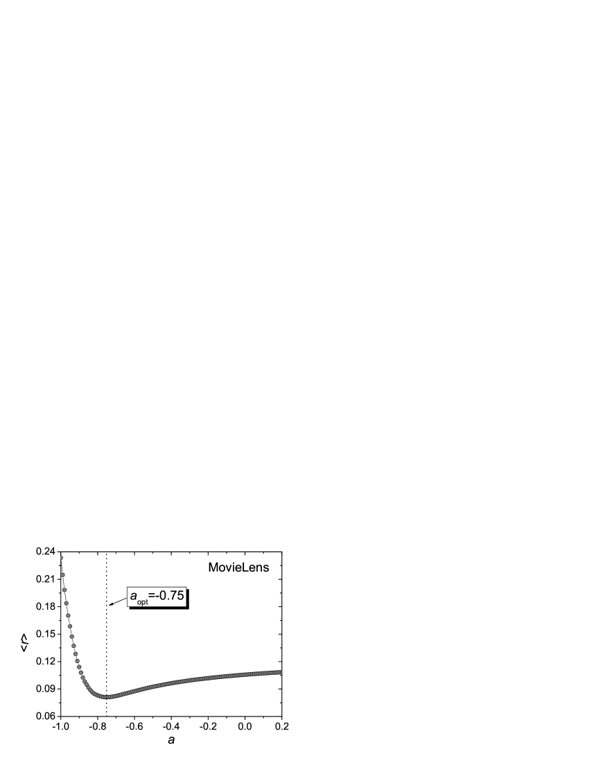
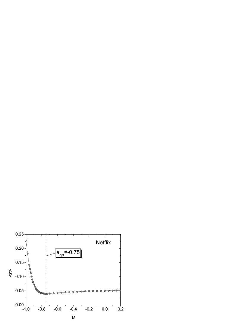
Figure 3: The ranking score $\langle r\rangle$ vs. $a$. The upper and lower plots shows the numerical results for MovieLens and Netflix, respectively. Each data point is obtained by averaging over five runs, each of which has an independently random division of training set and probe. Interestingly, for both MovieLens and Netflix, the optimal $a$, corresponding to the minimal $\langle r\rangle$, is $a_{\texttt{opt}}\approx-0.75$.

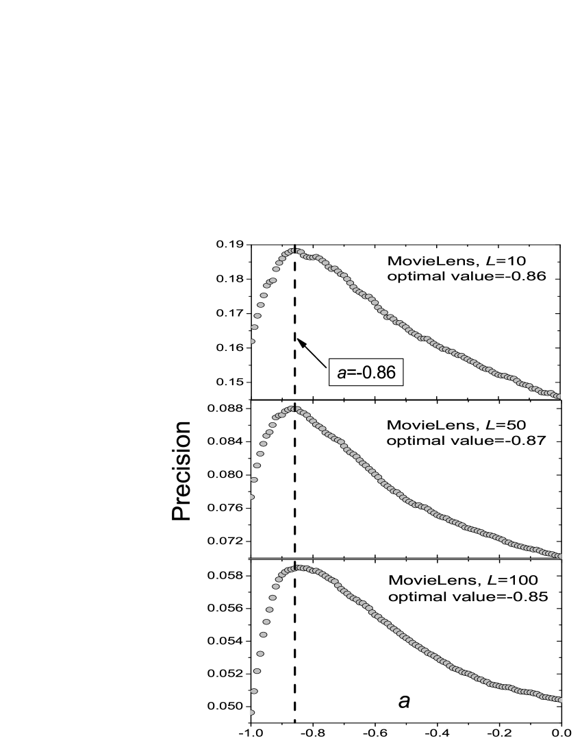
Figure 4: The precision vs. $a$ on MovieLens data for some typical lengths of recommendation list. Each data point is obtained by averaging over five runs, each of which has an independently random division of training set and probe.

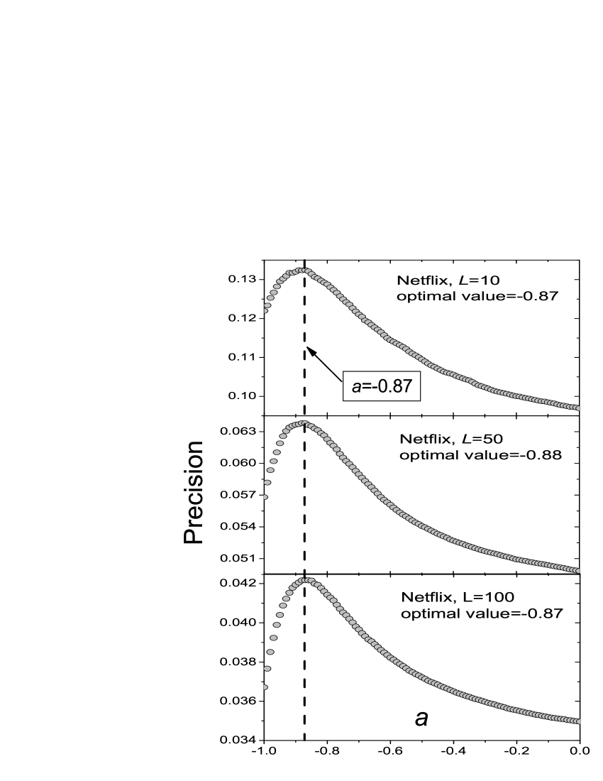
Figure 5: The precision vs. $a$ on Netflix data for some typical lengths of recommendation list. Each data point is obtained by averaging over five runs, each of which has an independently random division of training set and probe.

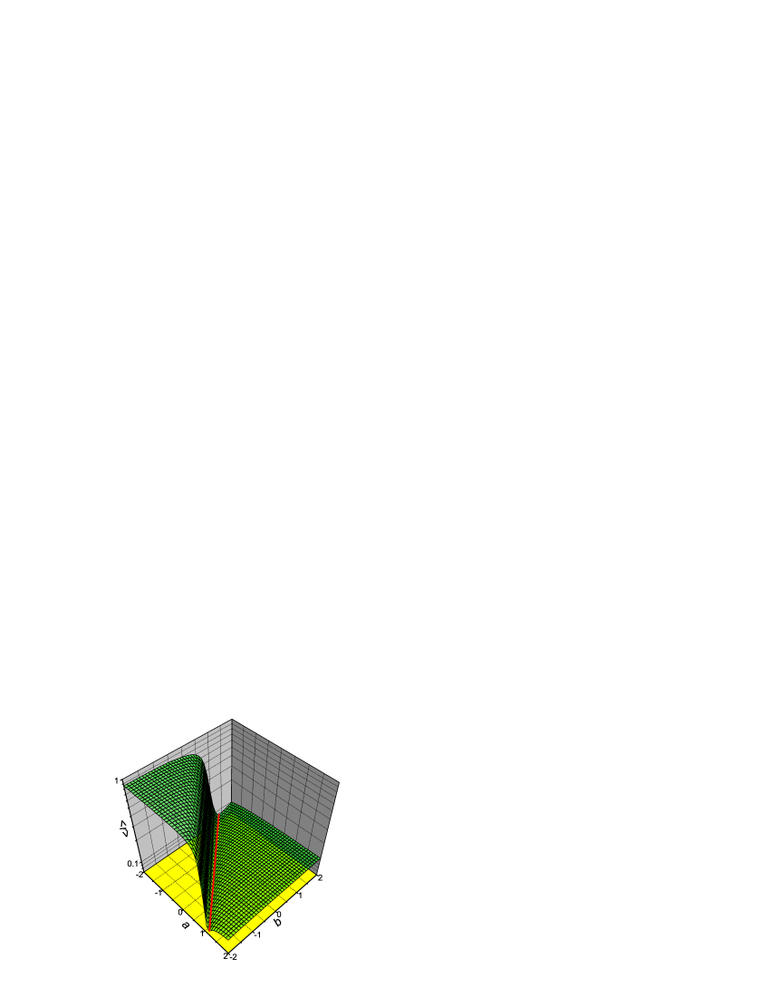
Figure 6: The ranking score $\langle r\rangle$ in $(a,b)$ plane for MovieLens data. The numerical simulations run over the parameters, $a$ and $b$, in the interval $[-2,2]$ and $[-2,2]$ respectively, with step length equaling 0.1. To make the figure clearer, the axis of $\langle r\rangle$ is set to be logarithmic. Given $a$, denoting $b^{*}(a)$ the optimal value of $b$ corresponding to the smallest $\langle r\rangle$. The red thick line emphasizes approximately the function $b^{*}(a)$. All the numerical results are obtained by averaging over five independent runs with data division identical to the case shown in Figure 3. The global minimum is $\langle r\rangle\approx 0.0794$, corresponding to $(a^{*},b^{*})=(-1.6,0.8)$.

For both C and F, the final recommendation value is two. However, according to our assumption, the target user likes C more than F. It is because in Fig. 2(a), the recommendations from A and B are independent, resulted from two different attributes; while in Fig. 2(b), the recommendations resulting from the same attribute (i.e., color=black) are repeatedly counted twice. Indeed, when calculating the recommendation value of F, the correlations D-F and E-F are redundant for each other. Although the real recommendation systems are much complicated than the simple example shown in Fig. 2, and no clear classification of objects’ attributes as well as no accurately quantitative measurements of users’ tastes can be extracted, we believe the redundance of correlations is ubiquity in those systems, which depresses the accuracy of NBI.

Note that, in Fig. 2(a), A and B, sharing no common property, do not have any correlation (in real system, two objects, even without any common/similar property, may have a certain weak correlation induced by occasional collections). While in Fig. 2(b), D and E are tightly connected for their common attribute, color=black, which is also the very causer of redundant recommendations to F. Therefore, following the path D$\rightarrow$E$\rightarrow$F, D and F have strong second-order correlation. However, since the correlation between A and B are very weak, the second-order correlation between A and C, contributed by the path A$\rightarrow$B$\rightarrow$C, should be neglectable.

Generally speaking, if the correlation between $o_{i}$ and $o_{k}$ and the correlation between $o_{j}$ and $o_{k}$ contain some redundance to each other, then the second-order correlation between $o_{i}$ and $o_{k}$, as well as that between $o_{j}$ and $o_{k}$ should be strong. Accordingly, subtracting the higher order correlations in an appropriate way could, perhaps, further improve the algorithmic accuracy. Motivated by this idea, we replace Eq. (5) by

$$\mathbf{f}^{\prime}=(W+aW^{2})\mathbf{f},$$ (13)

where $a$ is a free parameter. When $a=0$, it degenerates to the standard NBI discussed in the last section. If the present analysis is reasonable, the algorithm with a certain negative $a$ could outperforms the case with $a=0$.

Figure 3 reports the algorithmic accuracy, measured by the ranking score, as a function of $a$, which has a clear minimum around $a=-0.75$ for both MovieLens and Netflix. Compared with the standard case (i.e., $a=0$), the ranking score can be further reduced by 23% for MovieLens and 22% for Netflix, respectively. This result strongly supports our analysis. It is worthwhile to emphasize that, more than 20% is indeed a great improvement for recommendation algorithms. In addition, we compare the present algorithm with the Latent Dirichlet Allocation (LDA) algorithm [25], which is widely accepted as one of the most accurate personalized recommendation algorithms thus far. Although LDA requires much more computational time, the ranking score for MovieLens data is about 0.088, remarkably larger than the minimum, 0.082, obtained by the present algorithm. The ultra accuracy of the present method, even far beyond our expectation, indicates a great significance in potential applications. In addition, in Fig. 4 and Fig. 5, we present how the parameter $a$ affects the precision for some typical lengths of recommendation list. Although the optimal value of $a$ leading to the highest precision is different from the one subject to the lowest ranking score, the qualitative behaviors of $\langle r\rangle$ versus $a$ and $P(L)$ versus $a$ are the same, that is, in each case, there exists a certain negative $a$ corresponding to the most accurate recommendations (subject to the specific accuracy metric) with remarkable improvement compared with the standard NBI at $a=0$. We compare the ranking score and precision for $L=50$ in Table 1 and Table 2, where the Heter-NBI represents an improved NBI algorithm with heterogenous initial resource distribution [18], and RE-NBI is the current algorithm. To be fair to compare with parameter-free algorithms, in both Heter-NBI and RE-NBI, the parameters are fixed as the ones corresponding to the lowest ranking score, therefore the precisions presented in Table 1 and Table 2 are smaller than the optima. Even so, the present algorithm give much more accurate recommendations than all others.

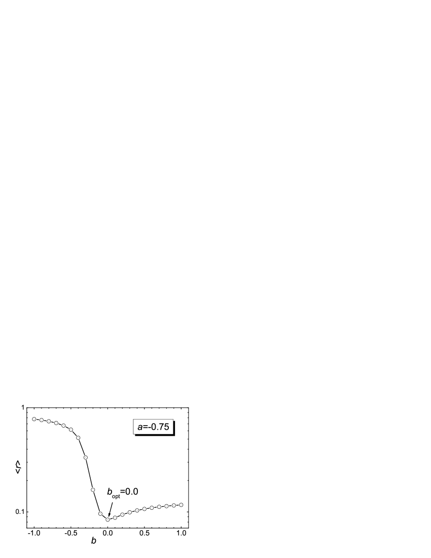
Figure 7: The ranking score $\langle r\rangle$ vs. $b$ given $a=-0.75$ for MovieLens data. All the numerical results are obtained by averaging over five independent runs with data division identical to the case shown in Fig. 3. The optimal value of $b$ is zero.

Although without a clear physical picture, Eq. (13) can be naturally extended to a formula containing even higher order of correlations than $W^{2}$, such as

$$\mathbf{f}^{\prime}=(W+aW^{2}+bW^{3})\mathbf{f},$$ (14)

where $b$ is also a free parameter. Since the computational complexity increases quickly as the increasing of the highest order of $W$, one should check very carefully if such kind of extension is valuable.

Extensively numerical simulations have been done to search the global minimum of $\langle r\rangle$ in $(a,b)$ plane for MovieLens data. Given $a$, denoting $b^{*}(a)$ the optimal value of $b$ corresponding to the smallest $\langle r\rangle$, as shown in Fig. 6 (red thick line), $b^{*}(a)$ decreases with the increasing of $a$ in aa approximately linear way. The global minimum of $\langle r\rangle$ is about 0.0794, corresponding to $(a^{*},b^{*})=(-1.6,0.8)$. That is to say, taking into account the cube of $W$, the algorithmic accuracy can be further improved by about 3%. However, the readers should be warned that the optimal parameters, $a^{*}$ and $b^{*}$, may be far different for different systems, and finding out them will take very long time for huge size systems. Therefore, the algorithm concerning three or even higher order of weighted matrix may be not applicable in real systems.

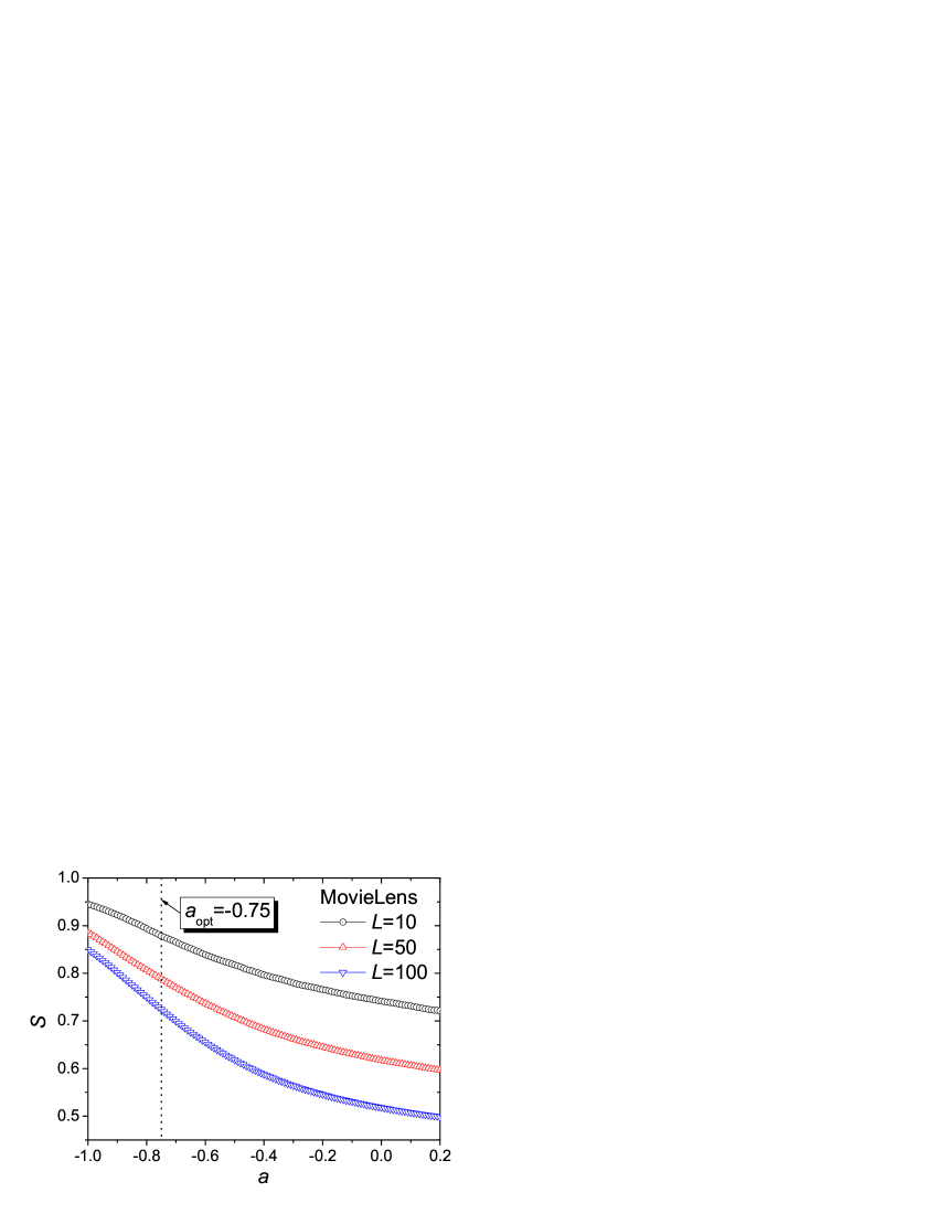
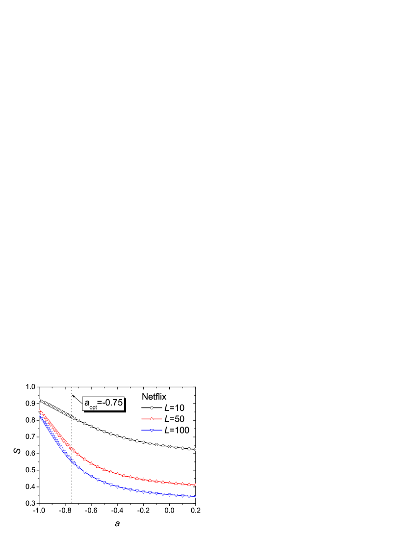
Figure 8: The Hamming distance, $S$, as a function of $a$. The black circles, red up-triangles and blue down-triangles represent the cases with typical lengths $L=10$, 50 and 100, respectively. The upper and lower plots correspond to the results on MovieLens and Netflix, respectively. The vertical line marks the optimal value of $a$, as $a_{\texttt{opt}}=-0.75$. All the numerical results are obtained by averaging over five independent runs with data division identical to the case shown in Figure 3.

Instead of the global search in $(a,b)$ plane, a possible way to quickly find out a nearly minimal $\langle r\rangle$ is using a greedy algorithm containing two steps. First, we search the optimal $a$ considering only the square of $W$, as shown in Eq. (13). Then, we search the optimal $b$ with $a$ fixed as the optimal value obtained in the first step. Clearly, this greedy method runs much faster than the blinding search in $(a,b)$ plane. However, as shown in Fig. 7, for MovieLens data with $a_{\texttt{opt}}=-0.75$, the optimal $b$ is zero, giving no improvement of the algorithm shown in Eq. (13). Therefore, though the introduction of two order correlation can greatly improve the algorithmic accuracy, to consider three or even higher order of $W$ may be not valuable.

4 Popularity and Diversity of Recommendations

When judging the algorithmic performance, most of the previous works only consider the accuracy of recommendations. Those measurements include [9, 10, 16, 26] ranking score, hitting rate, precision, recall, F-measure, and so on. However, besides accuracy, two significant ingredients must be taken into account. Firstly, the algorithm should guarantee the diversity of recommendations, viz., different users should be recommended different objects. It is also the soul of personalized recommendations. The inter-diversity can be quantified via the Hamming distance [18]. Denoting $L$ the length of recommendation list (i.e., the number of objects recommended to each user), if the overlapped number of objects in $u_{i}$ and $u_{j}$’s recommendation lists is $Q$, their Hamming distance is defined as

$$H_{ij}=1-Q/L.$$ (15)

Generally speaking, a more personalized recommendation list should have larger Hamming distances to other lists. Accordingly, we use the mean value of Hamming distance,

$$S=\frac{1}{m(m-1)}\sum_{i\neq j}H_{ij},$$ (16)

averaged over all the user-user pairs, to measure the diversity of recommendations. Note that, $S$ only takes into account the diversity among users. Besides, a good algorithm should also make the recommendations to a single user diverse to some extent [27], otherwise users may feel tired for receiving many recommended objects under the same topic. Motivated by Ziegler et al. [27], for an arbitrary target user $u_{l}$, denoting the recommended objects for $u_{l}$ as $\{o_{1},o_{2},\cdots,o_{L}\}$, the intra-similarity of $u_{l}$’s recommendation list can be defined as:

$$I_{l}=\frac{1}{L(L-1)}\sum_{i\neq j}s^{o}_{ij},$$ (17)

where $s^{o}_{ij}$ is the similarity between objects $o_{i}$ and $o_{j}$, as shown in Eq. (8). The intra-similarity of the whole system is thus defined as:

$$I=\frac{1}{m}\sum^{m}_{l=1}I_{l}.$$ (18)

In this paper, we use $S$ and $I$ respectively quantify the diversities among recommendation lists and inside a recommendation list.

Secondly, with more or less the same accuracy, an algorithm that recommends less popular objects is better than the one recommending popular objects. Taking recommender systems for movies as an example, since there are countless channels to obtain information of popular movies (TV, the Internet, newspapers, radio, etc.), uncovering very specific preference, corresponding to unpopular objects, is much more significant than simply picking out what a user likes from the top-viewed movies. The popularity can be directly measured by the average degree $\langle k\rangle$ over all the recommended objects.

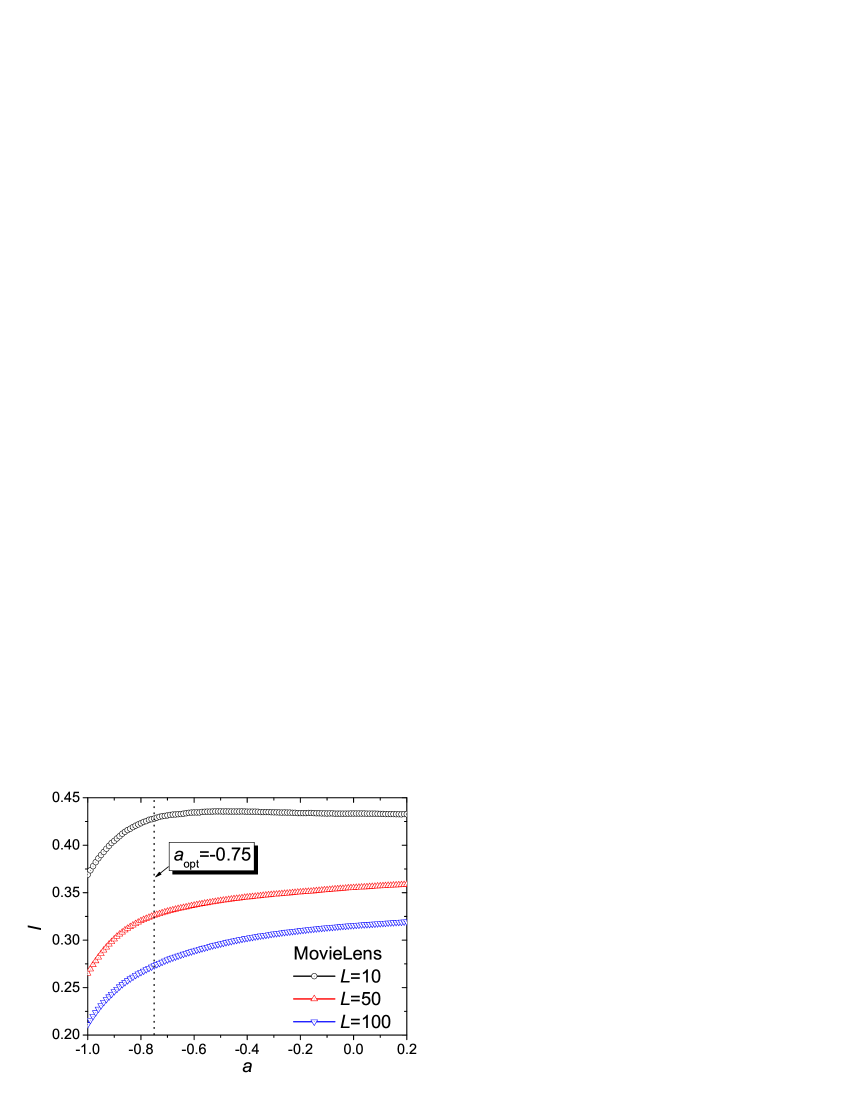
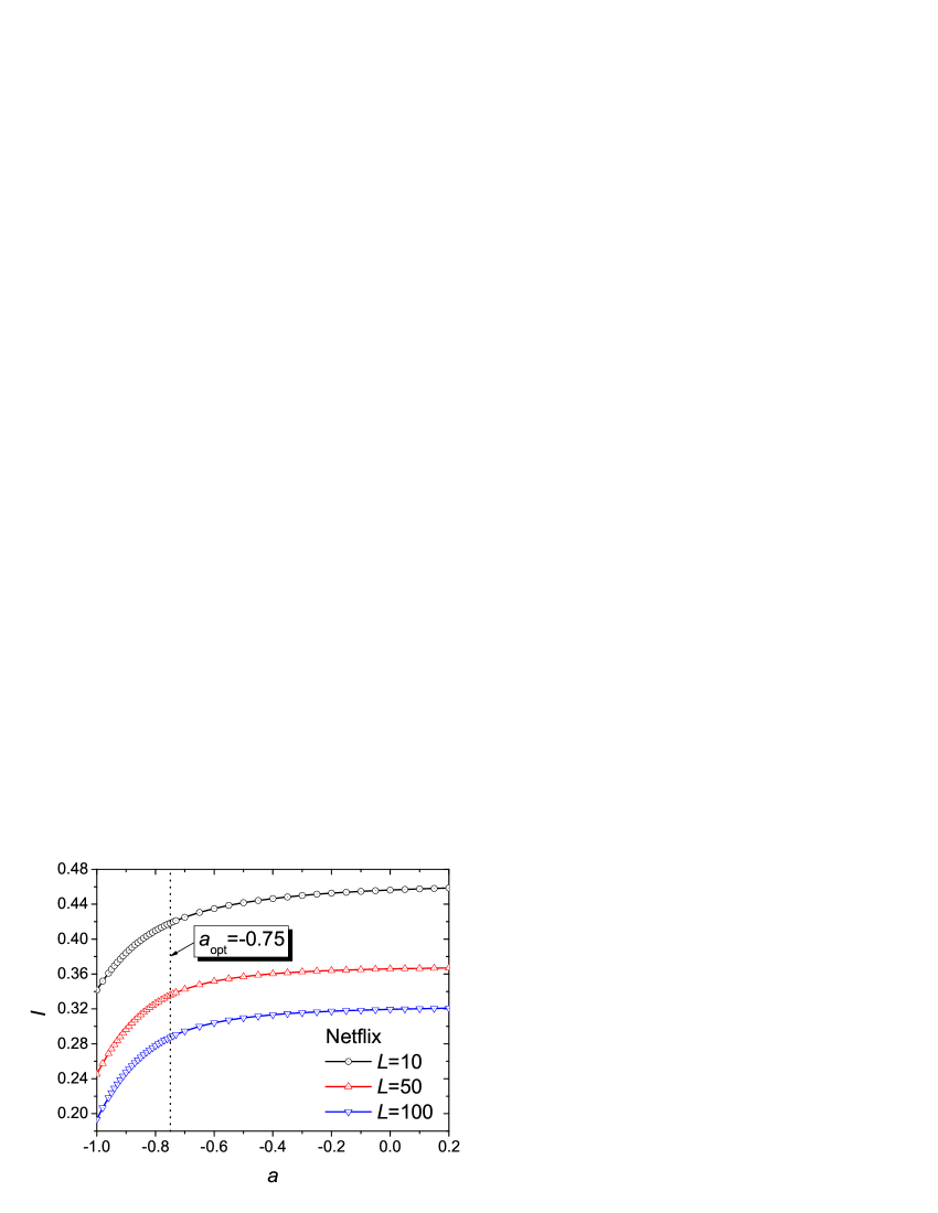
Figure 9: The intra-similarity, $I$, as a function of $a$. The black circles, red up-triangles and blue down-triangles represent the cases with typical lengths $L=10$, 50 and 100, respectively. The upper and lower plots correspond to the results on MovieLens and Netflix, respectively. The vertical line marks the optimal value of $a$, as $a_{\texttt{opt}}=-0.75$. All the numerical results are obtained by averaging over five independent runs with data division identical to the case shown in Figure 3.

Statistically speaking, the recommendations displaying high inter-diversity (i.e., large $S$) will have small popularity. It is because those high-degree objects (i.e., popular objects) are always the minority in a real system, and highly diverse recommendation lists must involve many less popular objects, thus depress the average degree $\langle k\rangle$. In contrast, a smaller $\langle k\rangle$ does not guarantee a higher $S$. An extreme example is to recommend every user the uncollected objects with minimal degrees. Therefore the average degree reaches its minimum, while the Hamming distance is close to zero since the recommendations to every user are almost the same. Therefore, $S$ of recommendations provides more information for the algorithmic performance than $\langle k\rangle$. However, the calculation of $S$ takes much longer time than that of $\langle k\rangle$, especially for a system containing quite a number of users. In addition, the definition of popularity is simpler and more intuitional than Hamming distance. In comparison, the intra-similarity, $I$, mainly concerning the underlying content of objects (two objects with similar content or in the same category usually have high probability to be collected by same users), is not directly relevant to the popularity. Therefore, we user all the three metrics here to provide comprehensive evaluation. In a word, besides the accuracy, an algorithm giving higher $S$, lower $I$ and lower $\langle k\rangle$ is more favorable.

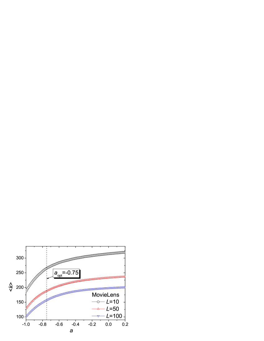
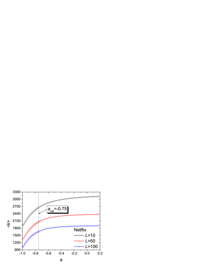
Figure 10: The average degree, $\langle k\rangle$, as a function of $a$. The black circles, red up-triangles and blue down-triangles represent the cases with typical lengths $L=10$, 50 and 100, respectively. The upper and lower plots correspond to the results on MovieLens and Netflix, respectively. The vertical line marks the optimal value of $a$, as $a_{\texttt{opt}}=-0.75$. All the numerical results are obtained by averaging over five independent runs with data division identical to the case shown in Figure 3.

In Fig. 8, we report the numerical results about how the parameter $a$ affects the Hamming distance, $S$. From this figure, one can see that the behaviors of $S(a)$ for both MovieLens and Netflix, as well as for different $L$, are qualitatively the same, namely $S$ is negatively correlated with $a$: the smaller $a$ the higher $S$. As a result, the present algorithm with $a=-0.75$ can provide obviously higher inter-diverse recommendations compared with the standard NBI at $a=0$. Figure 9 and Figure 10 show how the parameter $a$ affects the intra-similarity $I$ and the popularity $\langle k\rangle$, respectively. Clearly, the smaller $a$ leads to less intra-similarity and popularity, and thus the present algorithm can find its advantage in recommending less popular objects with diverse topics to users, compared with the standard NBI. Generally speaking, the popular objects must have some attributes fitting the tastes of the masses of the people. The standard NBI may repeatedly count those attributes and thus give overstrong recommendation for the popular objects, which increases the average degree of recommendations, as well as reduces the diversity. The collaborative filtering, considering only the first-order correlations, has the same problem as the standard NBI. The present algorithm with negative $a$ can to some extent eliminate the redundant correlations, namely assigns lower weights to the everyone-like attributes, and thus give higher chances to less popular objects and the objects with diverse topics different from the mainstream.

We summary the algorithmic performance in Table 1 and Table 2. One can find that in the case $a=-0.75$, the present algorithm outperforms the standard network-based inference (NBI) (i.e., $a=0$) [16] and its variant with heterogenous initial resource distribution (Heter-NBI) [18] in all five criteria: lower ranking score, higher precision, larger Hamming distance, lower intra-similarity and smaller average degree.

5 Conclusion and Discussion

The network-based inference [16], as introduced in Section 2, has higher accuracy as well as lower computational complexity than the widest personalized recommendation algorithm, namely the user-based collaborative filtering. Therefore, it has great potential significance in practical purpose. However, in this paper, we point out that in the NBI, the correlations resulting from a specific attribute may be repeatedly counted in the cumulative recommendations from different objects. Those redundant correlations will depress the algorithmic accuracy. By considering the higher order correlations, $W^{2}$, we design an effective algorithm that can, to some extent, eliminate the redundant correlations. The algorithmic accuracy, measured by the ranking score, can be further improved by 23% for MovieLens data and 22% for Netflix data in the optimal case at $a=-0.75$. Since the algorithm considering even higher order of $W$ takes too long time to be applied in real systems, and the improvement is not much as shown in Fig. 6 and Fig. 7, we suggest the readers taking into account $W$ and $W^{2}$ only. The current method can also be naturally extended to deal with the multi-rating recommender systems (see Ref. [17] a diffusion-like algorithm for multi-rating recommender systems). Indeed, the numerical simulations on the Netflix data with ratings show that considering the second-order correlations in building the transfer matrix can also improve the prediction accuracy (the method are more complicated than the binary systems present in this paper, see Ref. [17] for details).

Most of the previous studies considered the algorithmic accuracy only. Here, we argue that the diversity and popularity, as the significant criteria of algorithmic performance, should also be taken into account. Diversity is the soul of a personalized recommendation algorithm, that is to say, different users should be recommended, in general, different objects, and for a single user, the objects recommended to him should contain diverse topics. In addition, the recommendations of less popular objects are very significant in the modern information era, since those objects, even perfectly match a user’s tastes, could never be found out by this user himself from countless congeneric objects (e.g., millions of books and billions of webs). Without recommendation algorithm, those very less popular objects look like the dark information for normal users. Therefore, the algorithm that can provide accurate recommendations for less popular objects can be considered as a powerful tool uncovering the dark information. In a word, with more or less the same accuracy, an algorithm giving higher diversity and lower popularity is more favorable, and the numerical results show that the present algorithm can outperform the standard NBI and both the user-based and object-based collaborative filtering algorithms simultaneously in all five criteria: lower ranking score, higher precision, larger Hamming distance, lower intra-similarity and smaller average degree.

How to better provide personalized recommendations is a long-standing challenge in modern information science. Any answer to this question may intensively change our society, economic and life style in the near future. We believe the current work can enlighten readers in this interesting and exciting direction.

References

References

- [1] Zhang G Q, Zhang G Q, Yang Q F, Cheng S Q and Zhou T 2008 New J. Phys. 10 123027
- [2] Broder A, Kumar R, Moghoul F, Raghavan P, Rajagopalan S, Stata R, Tomkins A and Wiener J 2000 Comput. Netw. 33 309
- [3] Brin S and Page L 1998 Comput. Netw. ISDN Syst. 30 107
- [4] Kleinberg J M 1999 J. ACM 46 604
- [5] Linden G, Smith B and York J 2003 IEEE Internet Computing 7 76
- [6] Billsus D, Brunk C A, Evans C, Gladish B and Pazzani M J 2002 Commun. ACM 45 34
- [7] Ali K and van Stam W 2004 Proc. 10th ACM SIGKDD 394
- [8] Schafer J B, Konstan J A and Riedl J T 2001 Data Min. Knowl. Disc. 5 115
- [9] Adomavicius G and Tuzhilin A 2005 IEEE Trans. Knowl. Data Eng. 17 734
- [10] Herlocker J L, Konstan J A, Terveen K and Riedl J T 2004 ACM Trans. Inform. Syst. 22 5
- [11] Pazzani M J and Billsus D 2007 Lect. Notes Comput. Sci. 4321 325
- [12] Maslov S and Zhang Y C 2001 Phys. Rev. Lett. 87 248701
- [13] Ren J, Zhou T and Zhang Y C 2008 EPL 82 58007
- [14] Goldberg K, Roeder T, Gupta D and Perkins C 2001 Inf. Retr. 4 133
- [15] Zhang Y C, Blattner M and Yu Y K 2007 Phys. Rev. Lett. 99 154301
- [16] Zhou T, Ren J, Medo M and Zhang Y C 2007 Phys. Rev. E 76 046115
- [17] Zhang Y C, Medo M, Ren J, Zhou T, Li T and Yang F 2007 EPL 80 68003
- [18] Zhou T, Jiang L L, Su R Q and Zhang Y C 2008 EPL 81 58004
- [19] Ou Q, Jin Y D, Zhou T, Wang B H and Yin B Q 2007 Phys. Rev. E 75 021102
- [20] Sørensen T 1948 Biol. Skr. 5 1
- [21] Liben-Nowell D and Kleinberg J 2007 J. Am. Soc. Inform. Sci. Technol. 58 1019
- [22] Zhou T, Lü L and Zhang Y C 2009 Eur. Phys. J. B (to be published)
- [23] Sarwar B, Karypis G, Konstan J A and Riedl J T 2001 Proc. 10th Intl. Conf. WWW 285
- [24] Liu R R, Jia C X, Zhou T, Sun D and Wang B H 2009 Physica A 388 462
- [25] Blei D M, Ng A Y and Jordan M I 2003 J. Mach. Learn. Res. 3 993
- [26] Huang Z, Chen H and Zeng D 2004 ACM Trans. Inf. Syst. 22 116
- [27] Ziegler C N, McNee S M, Knostan J A and Lausen G 2005 Proc. 14th Intl. Conf. WWW 22