TTP 08-09
SFB/CPP-08-30

Electroweak Corrections to the Charm Quark Contribution to $K^{+}\to\pi^{+}\nu\bar{\nu}$

Abstract

We compute the leading-log QED, the next-to-leading-log QED-QCD, and the electroweak corrections to the charm quark contribution relevant for the rare decay $K^{+}\to\pi^{+}\nu\bar{\nu}$. The corresponding parameter $P_{c}(X)$ is increased by up to $2\%$ with respect to the pure QCD estimate to $P_{c}(X)=0.372\pm 0.015$ for $m_{c}(m_{c})=(1.286\pm 0.013)\,\textrm{GeV}$, $\alpha_{s}(M_{Z})=0.1176\pm 0.0020$ and $|V_{us}|=0.2255$. For the branching ratio we find $B(K^{+}\to\pi^{+}\nu\bar{\nu})=(8.5\pm 0.7)\times 10^{-11}$, where the quoted uncertainty is dominated by the CKM elements.

1 Introduction

The rare decay $K^{+}\to\pi^{+}\nu\bar{\nu}$ is both theoretically very clean and highly sensitive to short-distance physics and thus plays an outstanding role among flavour-changing neutral current processes both in the standard model (SM) and its extensions [1, 2, 3]. Together with the process $K_{L}\to\pi^{0}\nu\bar{\nu}$ it provides a critical test for the Cabibbo-Kobayashi-Maskawa (CKM) mechanism of CP violation, while it probes operators generated by new physics at energy scales of several TeV [4].

In the SM the decay $K^{+}\to\pi^{+}\nu\bar{\nu}$ proceeds through $Z$-penguin and electroweak box diagrams of $\mathcal{O}(G_{F}^{2})$ which exhibit a power-like GIM mechanism. This implies that non-perturbative effects are severely suppressed and, related to this, that the low-energy effective Hamiltonian [5, 6]

$$\mathcal{H}_{\text{eff}}=\frac{4G_{F}}{\sqrt{2}}\frac{\alpha}{2\pi\sin^{2}\theta_{W}}\sum_{l=e,\mu,\tau}\left(\lambda_{c}X^{l}(x_{c})+\lambda_{t}X(x_{t})\right)(\bar{s}_{L}\gamma_{\mu}d_{L})(\bar{\nu_{l}}_{L}\gamma^{\mu}{\nu_{l}}_{L})$$ (1)

involves to an excellent approximation only a single effective operator. Here $G_{F}$ is the Fermi constant, $\alpha$ the electromagnetic coupling and $\theta_{W}$ the weak mixing angle. The sum is over all lepton flavours, $\lambda_{i}=V^{*}_{is}V_{id}$ comprises the CKM factors and $f_{L}$ represents left-handed fermion fields.

The function $X(x_{t})$, where $x_{t}=m_{t}^{2}(\mu_{t})/M_{W}^{2}$ and $m_{t}^{2}(\mu_{t})$ is the top quark $\overline{\textrm{MS}}$ mass, describes the matching contributions of internal top quarks to the operator in Eq. (1), where the matching is carried out at the scale $\mu_{t}=\mathcal{O}(m_{t})$. Sample diagrams are shown in Fig. 1.

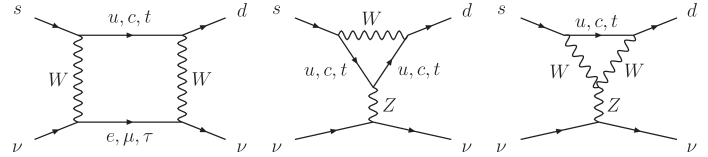
Figure 1: Examples of leading-order diagrams contributing to the decay $K^{+}\to\pi^{+}\nu\bar{\nu}$ in the SM.

The energy scales involved are of the order of the electroweak scale or higher, while both the QCD and QED anomalous dimensions of the corresponding operator vanish. Hence $X(x_{t})$ can be calculated within fixed-order perturbation theory. The relevant $Z$-penguin and electroweak box diagrams are known through next-to-leading order (NLO) in QCD [7, 8, 6, 9]. The inclusion of these $\mathcal{O}(\alpha_{s})$ corrections allowed to reduce the $\pm 6\%$ uncertainty related to the top quark matching scale $\mu_{t}=\mathcal{O}(m_{t})$ present in the leading order (LO) formula down to $\pm 1\%$. The leading term in the large top quark mass expansion of the electroweak two-loop corrections typically amounts to a per mil correction for the branching ratio if the $\overline{\textrm{MS}}$ definition of $\alpha$ and $\sin^{2}\theta_{W}$ is used, while the uncertainty related to unknown sub-leading electroweak contributions is conservatively estimated to be $\pm 2\%$ [10].

The function $X^{\ell}(x_{c})$, relevant only for $K^{+}\to\pi^{+}\nu\bar{\nu}$, depends on the charm quark $\overline{\textrm{MS}}$ mass through the parameter $x_{c}$, conventionally defined as

$$x_{c}=\frac{m_{c}^{2}(\mu_{c})}{M_{W}^{2}}\,.$$ (2)

As now both high-energy and low-energy scales, namely $\mu_{W}=\mathcal{O}(M_{W})$ and $\mu_{c}=\mathcal{O}(m_{c})$ are involved, a complete renormalisation group analysis of $X^{\ell}(x_{c})$ is required. In this manner, large logarithms $\ln(\mu_{c}^{2}/\mu_{W}^{2})$ are summed to all orders in $\alpha_{s}$. At LO such an analysis has been performed in [11]. The large scale uncertainty due to $\mu_{c}$ of $\pm 26\%$ in this result was reduced by a NLO [5, 6] and a subsequent NNLO calculation [12, 13, 14] to $\pm 2.5\%$. While the QCD part of the calculation has reached a high level of sophistication no QED or electroweak corrections have been included so far. We close this gap by calculating the LO and NLO logarithmic QED corrections as well as fixing the scheme of the input parameters in $\sin^{2}\theta_{W}$ and $\alpha$ by an electroweak matching calculation. The latter point can be exemplified by noting that the charm quark contribution is mediated by a double insertion of two dimension-six operators. This results in a contribution of $\mathcal{O}(G_{F}^{2})$ – the second power of $G_{F}$ resides in $x_{c}$ – plus electroweak corrections. Yet the leading result of Eq. (1) can only approximate the electroweak corrections for a specific choice of the renormalisation scheme for the prefactor of the charm quark contribution, expressed as $\alpha/\sin^{2}\theta_{W}$. While it is expected that using $\overline{\textrm{MS}}$ parameters renormalised at the electroweak scale would approximate the electroweak corrections best [15] only an explicit calculation can provide a definite result. In this work we normalise all dimension-six operators to $G_{F}$. Thus, we replace the parameter $x_{c}$ in Eq. (2) with the unfamiliar definition

$$x_{c}=\sqrt{2}\frac{\sin^{2}\theta_{W}}{\pi\alpha}G_{F}m_{c}^{2}(\mu_{c})\,,$$ (3)

which only at tree level equals the familiar ratio $m_{c}^{2}(\mu_{c})/M_{W}^{2}$.

The hadronic matrix element of the low-energy effective Hamiltonian can be extracted from the well-measured $K_{l3}$ decays, including isospin breaking and long-distance QED radiative corrections [16, 17, 18]. After summation over the three neutrino flavours the resulting branching ratio for $K^{+}\to\pi^{+}\nu\bar{\nu}$ can be written as [5, 6, 19]

$$B\left(K^{+}\to\pi^{+}\nu\bar{\nu}(\gamma)\right)\\ =\kappa_{+}(1+\Delta_{\text{EM}})\Bigg{[}\left(\frac{\text{Im}\lambda_{t}}{\lambda^{5}}X(x_{t})\right)^{2}+\left(\frac{\text{Re}\lambda_{c}}{\lambda}\left(P_{c}(X)+\delta P_{c,u}\right)+\frac{\text{Re}\lambda_{t}}{\lambda^{5}}X(x_{t})\right)^{2}\Bigg{]}.$$ (4)

The parameter

$$P_{c}(X)=\frac{1}{\lambda^{4}}\left(\frac{2}{3}X^{e}(x_{c})+\frac{1}{3}X^{\tau}(x_{c})\right)$$ (5)

describes the short-distance contribution of the charm quark, where $\lambda=\left|V_{us}\right|$. The charm quark contribution of dimension-eight operators at the charm quark scale $\mu_{c}$ combined with long distance contributions were calculated in Ref. [19] to be

$$\delta P_{c,u}=0.04\pm 0.02\,.$$ (6)

The quoted error on this value can in principle be reduced with the help of lattice QCD [20].

The remaining long distance corrections are factored out into the following two parameters: $\kappa_{+}$ contains higher-order electroweak corrections to the low energy matrix elements, and $\Delta_{\text{EM}}$ denotes long distance QED corrections. A detailed analysis of these contributions to NLO and partially NNLO in chiral perturbation theory has been performed by Mescia and Smith in [17], who found the numerical values $\kappa_{+}=(0.5173\pm 0.0025)\times 10^{-10}(\lambda/0.225)^{8}$ and $\Delta_{\text{EM}}=-0.3\%$.

2 Electroweak Corrections in the Charm Sector

The charm quark contribution involves several different scales and the corresponding large logarithms have to be summed using renormalisation group improved perturbation theory. Keeping terms to $\mathcal{O}(\alpha_{s})$ and $\mathcal{O}(\alpha/\alpha_{s})$ the expansion of the parameter $P_{c}(X)$ reads

$$P_{c}(X)=\frac{4\pi}{\alpha_{s}(\mu_{c})}P_{c}^{(0)}(X)+P_{c}^{(1)}(X)+\frac{\alpha_{s}(\mu_{c})}{4\pi}P_{c}^{(2)}(X)+\frac{4\pi\alpha}{\alpha_{s}^{2}(\mu_{c})}P_{c}^{(e)}(X)+\frac{\alpha}{\alpha_{s}(\mu_{c})}P_{c}^{(es)}(X).$$ (7)

The LO term $P_{c}^{(0)}(X)$, the NLO term $P_{c}^{(1)}(X)$, and the NNLO term $P_{c}^{(2)}(X)$ have been calculated in [11], in [5, 6], and in [14] respectively. The main goal of the this paper is to present the electroweak corrections $P_{c}^{(e)}(X)$ and $P_{c}^{(es)}(X)$.

The calculation is performed in two steps. First, at the scale $\mu_{W}\approx M_{W}$ the SM is matched to an effective theory where the top quark, the $W$ boson, and the $Z$ boson are integrated out, but the charm quark is still a dynamical degree of freedom. Second, at the scale $\mu_{c}\approx m_{c}$ the charm quark is integrated out and the effective Hamiltonian in Eq. (1) is obtained.

After integrating out the particles at the electroweak scale the effective Hamiltonian containing the dimension-six operators takes the following form:

$$\begin{split}\mathcal{H}_{\text{eff}}^{\text{dim.6}}=\frac{4G_{F}}{\sqrt{2}}\bigg{(}C_{W}(\mu)\sum_{q=u,c}(V_{qs}Q_{3q}+V_{qd}^{\star}Q_{4q})&\\ +\lambda_{c}\sum_{j=\pm}C_{j}(\mu)(Q_{j}^{c}-Q_{j}^{u})&+\frac{1}{2}C_{A}(\mu)Q_{A}+\frac{1}{2}C_{V}(\mu)Q_{V}\bigg{)}.\end{split}$$ (8)

Here we kept only operators relevant for the decay $K^{+}\to\pi^{+}\nu\bar{\nu}$. These are the semi-leptonic operators

$$Q_{3q}=\sum_{l=e,\mu,\tau}(\bar{s}_{L}\gamma_{\mu}q_{L})(\bar{\nu_{l}}_{L}\gamma^{\mu}l_{L})\quad\text{and}\quad Q_{4q}=\sum_{l=e,\mu,\tau}(\bar{q}_{L}\gamma_{\mu}d_{L})(\bar{l}_{L}\gamma^{\mu}{\nu_{l}}_{L})\,,$$ (9)

the current-current four-quark operators

$$Q_{\pm}^{q}=\frac{1}{2}\left((\bar{s}_{L}^{\alpha}\gamma_{\mu}q_{L}^{\alpha})(\bar{q}_{L}^{\beta}\gamma^{\mu}d_{L}^{\beta})\pm(\bar{s}_{L}^{\alpha}\gamma_{\mu}q_{L}^{\beta})(\bar{q}_{L}^{\beta}\gamma^{\mu}d_{L}^{\alpha})\right)\,,$$ (10)

where $\alpha$, $\beta$ are colour indices, and the operators

$$\begin{split}Q_{A}&=\sum_{q}\sum_{l=e,\mu,\tau}(-I_{q}^{3})(\bar{q}\gamma_{5}\gamma_{\mu}q)(\bar{\nu_{l}}_{L}\gamma^{\mu}{\nu_{l}}_{L})\,,\\ Q_{V}&=\sum_{q}\sum_{l=e,\mu,\tau}(I_{q}^{3}-2Q_{q}\sin^{2}\theta_{W})(\bar{q}\gamma_{\mu}q)(\bar{\nu_{l}}_{L}\gamma^{\mu}{\nu_{l}}_{L})\,,\end{split}$$ (11)

which describe the quark-neutrino interaction. We follow Ref. [14] in the definition of the evanescent operators. All evanescent operators relevant first at the order considered in this work are defined as

$$E_{3q}^{(1)}=\sum_{l=e,\mu,\tau}(\bar{s}_{L}\gamma_{\mu_{1}}\gamma_{\mu_{2}}\gamma_{\mu_{3}}q_{L})(\bar{\nu_{l}}_{L}\gamma^{\mu_{1}}\gamma^{\mu_{2}}\gamma^{\mu_{3}}l_{L})-(16-4\epsilon)Q_{3q}\,,$$ (12)

i.e. the evanescent operator needed for the QED renormalisation of $Q_{3q}$, or in an analogous way.

These operators mix via double insertions into the operator given in Eq. (1). Traditionally one distinguishes the box contribution which comprises double insertions of the semileptonic operators $Q_{3q}$ and $Q_{4q}$ (see Fig. 2, left side) and the penguin contribution which comprises double insertions of the current-current-type operators $Q_{\pm}$ and the operators $Q_{A}$ and $Q_{Z}$ (Fig. 2, right side). The relevant dimension-eight part of the effective Hamiltonian can then be written as

$$\mathcal{H}_{\text{eff}}^{\text{charm}}=\left(2G_{F}^{2}\lambda_{c}C_{\nu}^{B}(\mu)+G_{F}^{2}\lambda_{c}C_{\nu}^{P}(\mu)\right)Q_{\nu},$$ (13)

where the operator $Q_{\nu}$ is defined as

$$Q_{\nu}=\frac{m_{c}^{2}}{g_{s}^{2}\mu^{2\epsilon}}\sum_{l=e,\mu,\tau}(\bar{s}_{L}\gamma_{\mu_{1}}d_{L})(\bar{\nu_{l}}_{L}\gamma^{\mu_{1}}{\nu_{l}}_{L})\,,$$ (14)

while $C_{\nu}^{B}$ and $C_{\nu}^{P}$ denote the box and penguin contribution, respectively.

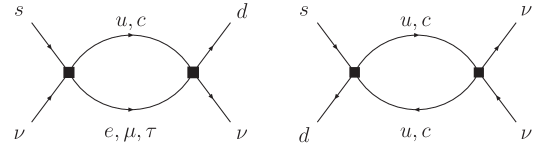
Figure 2: Leading-order diagrams for the mixing of various dimension-six operators into $Q_{\nu}$ (see text for details).

The renormalisation group analysis proceeds in several steps. The initial conditions for the renormalisation group equations (RGE), which govern the running of the Wilson coefficients, are calculated in Sec. 2.1. The anomalous dimensions are computed in Sec. 2.2. After integrating out the bottom and the charm quark, the theory is matched onto the low energy effective Hamiltonian of Eq. (1). The relevant results are collected in Sec. 2.3. In Sec. 2.4 the pieces are put together to give the final result for $P_{c}(X)$.

We have computed all Feynman diagrams in this paper using FORM [21] routines and independently using Mathematica. All the QCD corrections relevant to a NNLO analysis of $P_{c}(X)$ are given in [14] and references therein.

2.1 Initial Conditions

The Wilson coefficients are found by matching the one light particle irreducible Green’s functions in the full and the effective theory at the electroweak scale $\mu_{W}^{2}\sim M_{W}^{2}$. We use the $\overline{\textrm{MS}}$ scheme for both theories and remark that a finite field redefinition for the light particles ensures the correct normalisation of the kinetic term in the effective theory. In the box sector only $C_{W}$ and in the penguin sector only $C_{\pm}$ and $C_{A/V}$ receive electroweak corrections at the order considered here (see Fig. 3). We expand the Wilson coefficients in powers of the coupling constants

$$C(\mu)=C^{(0)}(\mu)+\frac{\alpha_{s}(\mu)}{4\pi}C^{(1)}(\mu)+\frac{\alpha}{\alpha_{s}}C^{(e)}(\mu)+\frac{\alpha}{4\pi}C^{(es)}(\mu)$$ (15)

and use a similar expansion for any quantity in the following, unless explicitly stated otherwise.

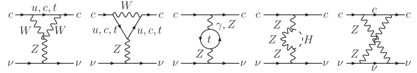
Figure 3: Feynman diagrams contributing to the NLO matching for $C_{A}$.

We normalise the Wilson coefficients $C_{W}$, $C_{\pm}$, and $C_{A/V}$ to the muon decay constant $G_{F}$ [22]. In this way most of the radiative corrections cancel, including all terms dependent on $m_{t}$ and $M_{H}$ in the case of $C_{W}$ and $C_{\pm}$. All our matching calculations have been performed in the generalised $R_{\xi}$ gauge for the photon field and in the case of $C_{A}$ also for the $W$ and $Z$ fields as a check of our results.

At the one-loop level a neutrino-photon Green’s function is generated which contributes to $C_{V}$ via the equations of motion. Yet $Q_{V}$ does not mix into $Q_{\nu}$ and the Wilson coefficient $C_{V}$ is not needed.

For the relevant electroweak corrections we find

$$\begin{split}C_{\pm}^{(0)}(\mu_{W})&=1\,,\\ C_{\pm}^{(e)}(\mu_{W})&=0\,,\\ C_{\pm}^{(es)}(\mu_{W})&=-\frac{22}{9}-\frac{4}{3}\ln\frac{\mu_{W}^{2}}{M_{Z}^{2}}\,,\end{split}$$ (16)

in agreement with Ref. [23, 24],

$$\begin{split}{C}_{W}^{(0)}(\mu_{W})&=1\,,\\ {C}_{W}^{(e)}(\mu_{W})&=0\,,\\ {C}_{W}^{(es)}(\mu_{W})&=-\frac{11}{3}-2\ln\frac{\mu_{W}^{2}}{M_{Z}^{2}}\,,\end{split}$$ (17)

and

$$\begin{split}C_{A}^{(0)}(\mu_{W})&=1\,,\\ C_{A}^{(e)}(\mu_{W})&=0\,,\\ C_{A}^{(es)}(\mu_{W})&=\frac{3m_{t}^{2}}{4s_{w}^{2}M_{W}^{2}}+\frac{11s_{w}^{2}-6}{4s_{w}^{2}c_{w}^{2}}-\frac{3}{4}\,\frac{M_{W}^{2}-c_{w}^{2}M_{H}^{2}}{(M_{H}^{2}-M_{W}^{2})s_{w}^{4}}\ln{\frac{M_{W}^{2}}{M_{Z}^{2}}}\\ &\quad+\frac{3M_{H}^{4}}{4(M_{H}^{2}-M_{W}^{2})(M_{W}^{2}-c_{w}^{2}M_{H}^{2})}\ln{\frac{M_{H}^{2}}{M_{Z}^{2}}}\,.\end{split}$$ (18)

2.2 Anomalous Dimensions and RGE

The mixing of dimension-six into dimension-eight operators through double insertions leads in general to inhomogeneous RGE [25]. In the box sector they are given by

$$\mu\frac{d}{d\mu}C_{\nu}^{B}(\mu) =\gamma_{\nu}C_{\nu}^{B}(\mu)+4\gamma_{\nu}^{B}C_{W}(\mu)C_{W}(\mu)\,,$$ (19)

$$\mu\frac{d}{d\mu}C_{W}(\mu) =\gamma_{W}C_{W}(\mu)\,,$$ (20)

where $\gamma_{W}$ is the anomalous dimension of $Q_{3q}$, $\gamma_{\nu}$ encodes the running of $Q_{\nu}$, which stems solely from the running mass and coupling constant which in our definition multiply the $Q_{\nu}$ operator, and $\gamma_{\nu}^{B}$ is the anomalous dimension tensor of the mixing of the operators $Q_{3q}$ and $Q_{4q}$ into $Q_{\nu}$.

$\gamma_{\nu}$ is given in terms of the QCD $\beta$-function and the anomalous dimension of the charm quark mass by

$$\gamma_{\nu}^{(k)}=2(\gamma_{m}^{(k)}-\beta_{k}).$$ (21)

The explicit values are

$$\gamma_{m}^{(0)}=8\,,\qquad\gamma_{m}^{(e)}=\frac{8}{3}\,,\qquad\gamma_{m}^{(es)}=\frac{32}{9}\,,$$ (22)

$$\beta_{0}=11-\frac{2}{3}f\,,\qquad\beta_{e}=0\,,\qquad\beta_{es}=-\frac{8}{9}(f_{u}+\frac{f_{d}}{4})\,,$$ (23)

where $f_{u}$ and $f_{d}$ denote the number of up- and down-type quark flavours, and $f=f_{u}+f_{d}$.

The remaining anomalous dimensions can be calculated from the pole parts of one- and two-loop diagrams, some of which are shown in Figs. 4 and 5, using standard methods [25, 26, 27].

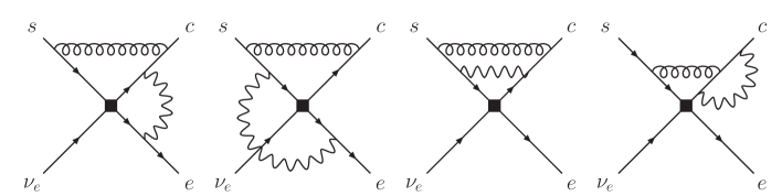
Figure 4: Sample two-loop diagrams contributing to the self mixing of $Q_{3c}$. Wavy lines denote photons, curly lines denote gluons.

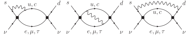
Figure 5: Sample diagrams for the NLO mixing of $Q_{3q}$ and $Q_{4q}$ into $Q_{\nu}$.

We find the following values:

$$\gamma_{\nu}^{B(0)}=-8\,,\qquad\gamma_{\nu}^{B(e)}=0\,,\qquad\gamma_{\nu}^{B(es)}=-\frac{316}{9}\,,$$ (24)

$$\gamma_{W}^{(0)}=0\,,\qquad\gamma_{W}^{(e)}=-4\,,\qquad\gamma_{W}^{(es)}=4\,.$$ (25)

$\gamma_{\nu}^{B(0)}$ is known for a long time (see [5] and references therein), and $\gamma_{W}^{(e)}$ and $\gamma_{W}^{(es)}$ have already been calculated in [22].

In order to solve the RGE we perform a trick [28, 5], so that we can use the RGE for single insertions also in our case. To this end, we rewrite Eq. (20) as

$$\mu\frac{d}{d\mu}C_{W}^{2}(\mu)=2\gamma_{W}^{T}C_{W}^{2}(\mu).$$ (26)

Then we can combine both equations (19) and (20) into a linear equation

$$\mu\frac{d}{d\mu}C_{B}(\mu)=\gamma_{B}^{T}C_{B}(\mu),$$ (27)

where

$$C_{B}(\mu)=\begin{pmatrix}4C_{W}^{2}(\mu)\\ C_{\nu}^{B}(\mu)\end{pmatrix}\quad\text{and}\quad\gamma_{B}^{T}=\begin{pmatrix}2\gamma_{W}&0\\ \gamma_{\nu}^{B}&\gamma_{\nu}\end{pmatrix}.$$ (28)

The RGE for the penguin sector are given by

$$\mu\frac{d}{d\mu}C_{\nu}^{P}(\mu) =\gamma_{\nu}C_{\nu}^{P}(\mu)+4\sum_{i=\pm}\gamma_{i,\nu}^{P}C_{i}(\mu)C_{A}(\mu),$$ (29)

$$\mu\frac{d}{d\mu}C_{\pm}(\mu) =\gamma_{\pm}^{T}C_{\pm}(\mu).$$ (30)

The anomalous dimension tensor $\gamma_{\pm,\nu}^{P}$ governs the mixing of the double insertion of $Q_{\pm}$ and $Q_{A}$ into $Q_{\nu}$ (see Fig. 6), while $\gamma_{\pm}$ describes the self-mixing of $Q_{\pm}$ and was computed in [29]. The anomalous dimensions read:

$$\gamma_{\pm,\nu}^{P(0)}=2(1\pm 3),\qquad\gamma_{\pm,\nu}^{P(e)}=0,\qquad\gamma_{\pm,\nu}^{P(es)}=\frac{52}{3}(1\pm 3).$$ (31)

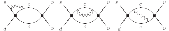
Figure 6: Sample diagrams for the NLO mixing of $Q_{A}$ and $Q_{\pm}$ into $Q_{\nu}$.

We have defined the matrix $\gamma_{\pm}^{P}$ as

$$\gamma_{\pm,\nu}^{P(k)}=-\frac{1}{2}\gamma_{\pm,\nu}^{A(k)}-\left(\frac{1}{2}-\frac{4}{3}\sin^{2}\theta_{W}\right)\gamma_{\pm,\nu}^{V(k)}\,,$$ (32)

with the superscripts $A$ and $V$ denoting the contributions stemming from double insertion of $(Q_{\pm}^{q},Q_{A}^{q})$ and $(Q_{\pm}^{q},Q_{V}^{q})$, respectively. The LO result agrees with [5, 14]. The other contributions are new.

The anomalous dimension of $Q_{A}$ vanishes and the RGE in the penguin sector is the linear equation

$$\mu\frac{d}{d\mu}C_{P}(\mu)=\gamma_{P}^{T}C_{P}(\mu),$$ (33)

where

$$C_{P}(\mu) =\begin{pmatrix}4C_{+}(\mu)C_{A}\\ 4C_{-}(\mu)C_{A}\\ C_{\nu}^{P}(\mu)\end{pmatrix}, \gamma_{P}^{T} =\begin{pmatrix}\gamma_{\pm}^{T}&{\begin{matrix}\gamma_{+,\nu}^{P}\\ \gamma_{-,\nu}^{P}\end{matrix}}\\ {\begin{matrix}0&0\end{matrix}}&\gamma_{\nu}\end{pmatrix}\,.$$ (34)

The RGE for single insertions can be solved explicitly using the method described in [30].

2.3 Below $\mu_{c}$

At $\mu_{c}$, i.e. the scale of the charm quark mass, the charm quark is integrated out and removed as a degree of freedom. All necessary matrix elements are given in [14, 5] – no new contributions arise to the orders considered here. There are some new terms stemming from the expansion of $m_{c}(\mu_{c})$ about $m_{c}(m_{c})$ in these expressions, though, and we collect these results for convenience.

The matching in the box sector leads to the following matrix elements:

$$r_{\tau}^{B(1)}(\mu_{c})=5+\frac{4x_{\tau}}{1-x_{\tau}}\ln x_{\tau}+4\ln\frac{\mu_{c}^{2}}{m_{c}^{2}},$$ (35)

where $x_{\tau}=m_{\tau}^{2}/m_{c}^{2}$ and $m_{c}=m_{c}(\mu_{c})$. Neglecting the lepton masses for the electron and muon, the above formula yields

$$r_{e,\mu}^{B(1)}(\mu_{c})=5+4\ln\frac{\mu_{c}^{2}}{m_{c}^{2}}.$$ (36)

We have defined the matrix elements for lepton flavour $l$ by

$$\langle Q_{l}^{B}(\mu_{c})\rangle=\frac{\alpha_{s}(\mu_{c})}{4\pi}r_{l}^{B(1)}(\mu_{c})\langle Q_{\nu}\rangle^{(0)},$$ (37)

where $\langle Q_{l}^{B}(\mu_{c})\rangle$ denotes the double insertion of the operators in the box sector. In the penguin sector we find

$$r_{\pm}^{P(1)}(\mu_{c})=(1\pm 3)\left(1-\ln\frac{\mu_{c}^{2}}{m_{c}^{2}}\right),$$ (38)

where

$$\langle Q_{\pm}^{P}(\mu_{c})\rangle=\frac{\alpha_{s}(\mu_{c})}{4\pi}r_{\pm}^{P(1)}(\mu_{c})\langle Q_{\nu}\rangle^{(0)},$$ (39)

and $\langle Q_{\pm}^{P}(\mu_{c})\rangle$ denotes the double insertion of the operators in the penguin sector.

2.4 Final Analytic Expression for $P_{c}(X)$

Now all that remains to do is to combine all relevant terms and compute the box and penguin contributions to the function $X^{l}(x_{c})$ defined in Eq. (1). Here we closely follow [14]. Let us start with the box contribution. We expand the result as

$$C_{B}^{l}(\mu_{c})=\kappa_{c}\frac{x_{c}(m_{c})}{16}\left(\frac{4\pi}{\alpha_{s}(\mu_{c})}C_{B}^{l(0)}(\mu_{c})+\frac{4\pi\alpha}{\alpha_{s}(\mu_{c})^{2}}C_{B}^{l(e)}(\mu_{c})+\frac{\alpha}{\alpha_{s}(\mu_{c})}C_{B}^{l(es)}(\mu_{c})\right)$$ (40)

and express the running charm quark mass $m_{c}(\mu_{c})$ in terms of initial condition $m_{c}(m_{c})$,

$$x_{c}(\mu_{c})=\kappa_{c}\left(1+\frac{\alpha_{s}(\mu_{c})}{4\pi}\xi_{c}^{(1)}+\frac{\alpha}{\alpha_{s}(\mu_{c})}\xi_{c}^{(e)}+\frac{\alpha}{4\pi}\xi_{c}^{(es)}\right)x_{c}(m_{c}),$$ (41)

where we defined $\kappa_{c}=\eta_{c}^{(\gamma^{(0)}_{m}/\beta_{0})}$ and $\eta_{c}=\alpha_{s}(\mu_{c})/\alpha_{s}(m_{c})$, with the individual contributions

$$\xi_{c}^{(1)} =\left(\frac{\gamma^{(1)}_{m}}{\beta_{0}}-\frac{\gamma^{(0)}_{m}\beta_{1}}{\beta_{0}^{2}}\right)(1-\eta_{c}^{-1})\,,$$

$$\xi_{c}^{(e)} =\frac{\gamma^{(e)}_{m}}{\beta_{0}}(\eta_{c}-1)\,,$$

$$\xi_{c}^{(es)} =\left(\frac{\gamma^{(es)}_{m}}{\beta_{0}}-\frac{\beta_{es}\gamma^{(0)}_{m}}{\beta_{0}^{2}}-\frac{\beta_{1}\gamma^{(e)}_{m}}{\beta_{0}^{2}}\right)\ln\eta_{c}$$

$$\quad+\frac{\gamma^{(e)}_{m}}{\beta_{0}}\left(\frac{\gamma^{(0)}_{m}\beta_{1}}{\beta_{0}^{2}}-\frac{\gamma^{(1)}_{m}}{\beta_{0}}\right)(1-\eta_{c}^{-1})(1-\eta_{c}).$$ (42)

We find the following expansion coefficients for $C_{B}^{l}$:

$$C_{B}^{l(0)}(\mu_{c}) =C_{\nu}^{B(0)}(\mu_{c}),$$

$$C_{B}^{l(e)}(\mu_{c}) =C_{\nu}^{B(e)}(\mu_{c})+C_{\nu}^{B(0)}(\mu_{c})\xi_{c}^{(e)}+4C_{W}^{(0)}(\mu_{c})^{2}\rho_{l}^{B(e)}(\mu_{c}),$$

$$C_{B}^{l(es)}(\mu_{c}) =C_{\nu}^{B(es)}(\mu_{c})+C_{\nu}^{B(e)}(\mu_{c})\xi_{c}^{(1)}+C_{\nu}^{B(1)}(\mu_{c})\xi_{c}^{(e)}+C_{\nu}^{B(0)}(\mu_{c})\xi_{c}^{(es)}$$

$$\quad+4C_{W}^{(0)}(\mu_{c})^{2}\rho_{l}^{B(es)}(\mu_{c})+4C_{W}^{(0)}(\mu_{c})^{2}\rho_{l}^{B(e)}(\mu_{c})\xi_{c}^{(1)}$$

$$\quad+8C_{W}^{(0)}(\mu_{c})C_{W}^{(e)}(\mu_{c})\rho_{l}^{B(1)}(\mu_{c})+4C_{W}^{(0)}(\mu_{c})^{2}\rho_{l}^{B(1)}(\mu_{c})\xi_{c}^{(e)}.$$ (43)

We obtain the parameters $\rho_{l}^{B}$ by inserting the expansion of $m_{c}(\mu_{c})$ into the expressions for $r_{l}^{B}$ (see Sec. 2.3):

$$\rho_{\tau}^{B(1)} =r_{\tau}^{B(1)}(m_{c})+\frac{4}{x_{\tau}-\kappa_{c}}\left(\kappa_{c}\ln\kappa_{c}-\frac{x_{\tau}(1-\kappa_{c})}{1-x_{\tau}}\ln x_{\tau}\right)\,,$$

$$\rho_{\tau}^{B(e)} =0\,,$$

$$\rho_{\tau}^{B(es)} =-\frac{4\kappa_{c}\xi_{c}^{(e)}\left[\kappa_{c}-x_{\tau}\left(1-\ln\frac{x_{\tau}}{\kappa_{c}}\right)\right]}{(\kappa_{c}-x_{\tau})^{2}}\,.$$ (44)

The corresponding expressions for the electron and the muon, where we can neglect the masses, are given by

$$\rho_{e,\mu}^{B(1)} =r_{e,\mu}^{B(1)}(m_{c})-4\ln\kappa_{c}\,,$$

$$\rho_{e,\mu}^{B(e)} =0\,,$$

$$\rho_{e,\mu}^{B(es)} =-4\xi_{c}^{(e)}\,.$$ (45)

The penguin contribution to the function $X^{l}(x_{c})$ can be obtained in the same way. Expanding the Wilson coefficients $C_{P}(\mu_{c})$ as

$$C_{P}(\mu_{c})=\kappa_{c}\frac{x_{c}(m_{c})}{32}\left(\frac{4\pi}{\alpha_{s}(\mu_{c})}C_{P}^{(0)}(\mu_{c})+\frac{4\pi\alpha}{\alpha_{s}(\mu_{c})^{2}}C_{P}^{(e)}(\mu_{c})+\frac{\alpha}{\alpha_{s}(\mu_{c})}C_{P}^{(es)}(\mu_{c})\right),$$ (46)

we find the following contributions:

$$C_{P}^{(0)}(\mu_{c}) =C_{\nu}^{P(0)}(\mu_{c}),$$

$$C_{P}^{(e)}(\mu_{c}) =C_{\nu}^{P(e)}(\mu_{c})+C_{\nu}^{P(0)}(\mu_{c})\xi_{c}^{(e)}+4C_{A}^{(0)}(\mu_{c})\sum_{i=\pm}C_{i}^{(0)}(\mu_{c})\rho_{i}^{P(e)}(\mu_{c}),$$

$$C_{P}^{(es)}(\mu_{c}) =C_{\nu}^{P(es)}(\mu_{c})+C_{\nu}^{P(e)}(\mu_{c})\xi_{c}^{(1)}+C_{\nu}^{P(1)}(\mu_{c})\xi_{c}^{(e)}+C_{\nu}^{P(0)}(\mu_{c})\xi_{c}^{(es)}$$

$$\quad+4\sum_{i=\pm}\left(\rho_{i}^{P(es)}(\mu_{c})+\rho_{i}^{P(e)}(\mu_{c})\xi_{c}^{(1)}+\rho_{i}^{P(1)}(\mu_{c})\xi_{c}^{(e)}\right)C_{i}^{(0)}(\mu_{c})C_{A}^{(0)}(\mu_{c})$$

$$\quad+4\sum_{i=\pm}\rho_{i}^{P(1)}(\mu_{c})\left(C_{i}^{(e)}(\mu_{c})C_{A}^{(0)}(\mu_{c})+C_{i}^{(0)}(\mu_{c})C_{A}^{(e)}(\mu_{c})\right)$$

$$\quad+4\sum_{i=\pm}\rho_{i}^{P(e)}(\mu_{c})C_{i}^{(1)}(\mu_{c})C_{A}^{(0)}(\mu_{c}).$$ (47)

Again we obtain the parameters $\rho_{i}^{P}$ by inserting the expansion of $m_{c}(\mu_{c})$ into the expressions for $r_{i}^{P}$:

$$\rho_{\pm}^{P(1)} =r_{\pm}^{P(1)}(m_{c})+(1\pm 3)\ln\kappa_{c},$$

$$\rho_{\pm}^{P(e)} =0,$$

$$\rho_{\pm}^{P(es)} =(1\pm 3)\xi_{c}^{(e)}.$$ (48)

The final result for $X^{l}$ is then

$$X^{l}(x_{c})=C_{P}(\mu_{c})+C_{B}^{l}(\mu_{c}).$$ (49)

The corresponding expressions for $C_{P}(\mu_{c})$ and $C_{B}^{l}(\mu_{c})$ can be found in Eqs. (40) and (46), respectively. Eq. (5) then yields the contribution to the branching fraction.

3 Final Results and Numerical Discussion

Having all necessary ingredients at hand we will discuss the numerical implications of our results, where we use the input parameters given in Tab. 1.

$M_{W}$	$(80.403\pm 0.029)$ GeV	[31]	$\alpha_{s}(M_{Z})$	$0.1176\pm 0.0020$	[31]
$M_{Z}$	$(91.1876\pm 0.0021)$ GeV	[31]	$\alpha(M_{Z})$	1/127.9	[31]
$M_{t}$	$(172.6\pm 1.4)$ GeV	[32]	$\sin^{2}\theta_{W}^{\overline{\text{MS}}}$	$0.23122\pm 0.00015$	[31]
$m_{b}(m_{b})$	$(4.164\pm 0.025)$ GeV	[33]	$G_{F}$	$1.166\,37\times 10^{-5}\text{GeV}^{-2}$	[31]
$m_{c}(m_{c})$	$(1.286\pm 0.013)$ GeV	[33]	$\lambda$	$0.2255\pm 0.0007$	[34]
$M_{H}$	$(155\pm 40)$ GeV	–	$\left|V_{cb}\right|$	$(4.15\pm 0.09)\times 10^{-2}$	[35]
$m_{\tau}$	$(1776.99^{+0.29}_{-0.26})$ MeV	[31]	$\bar{\rho}$	$0.141^{+0.029}_{-0.017}$	[35]
			$\bar{\eta}$	$0.343\pm 0.016$	[35]

Table 1: Input parameters used in our numerical analysis.

Our numerical procedure follows closely the one of Ref. [14]. In particular we use the numerical solution of the RGE of the program RunDec[36] to compute $\alpha_{s}(\mu_{c})$ from $\alpha_{s}(M_{Z})$ and neglect all terms proportional to $\beta_{es}$. We have checked numerically that this is indeed justified.

The dependence of $P_{c}(X)$ on the parameter $\mu_{c}$ can be seen in Fig. 7. We use central values for all relevant input parameters of Tab. 1 and fix $\mu_{b}=5\,$GeV and $\mu_{W}=80\,$GeV. The dashed line shows $P_{c}(X)$ as a function of $\mu_{c}$ including the NNLO QCD corrections, as computed in [14] where the parameter $x_{c}$ equals $m_{c}^{2}/M_{W}^{2}$. The dashed-dotted line shows the same quantity, but using our improved definition of $x_{c}$, see Eq. (3). We observe that this line is shifted by about 0.5% compared to $P_{c}(X)$ using the conventional definition of $x_{c}$. The dotted and the solid lines show the results including LO QED and the NLO electroweak corrections, respectively. We see that including the full electroweak corrections, $P_{c}(X)$ is increased by another 1.5% as compared to the pure NNLO QCD result with the improved definition of $x_{c}$. Also the cancellation of the scheme dependence between the LO QED and the NLO electroweak contribution is clearly visible.

Figure 7: $P_{c}(X)$ as a function of $\mu_{c}$ at NNLO QCD (dashed dotted line), including LO QED (dotted line), and NLO electroweak corrections (solid line). The dashed line shows $P_{c}(X)$ at NNLO QCD where the definition $x_{c}=m_{c}/M_{W}$ is used.

The explicit analytic expression for $P_{c}(X)$ including the complete NNLO corrections is so complicated and long that we derive an approximate formula. Setting $\lambda=0.2255$ and $m_{t}(m_{t})=163.0\textrm{GeV}$ we derive an approximate formula for $P_{c}(X)$ that summarises the dominant parametric and theoretical uncertainties due to $m_{c}(m_{c})$, $\alpha_{s}(M_{Z})$, $\mu_{c}$, $\mu_{W}$, and $\mu_{b}$. It reads

$$\begin{split}P_{c}(X)&=0.38049\left(\frac{m_{c}(m_{c})}{1.30\textrm{GeV}}\right)^{0.5081}\left(\frac{\alpha_{s}(M_{Z})}{0.1176}\right)^{1.0192}\left(1+\sum_{i,j}\kappa_{ij}L_{m_{c}}^{i}L_{\alpha_{s}}^{j}\right)\\ &\pm 0.008707\left(\frac{m_{c}(m_{c})}{1.30\textrm{GeV}}\right)^{0.5276}\left(\frac{\alpha_{s}(M_{Z})}{0.1176}\right)^{1.8970}\left(1+\sum_{i,j}\epsilon_{ij}L_{m_{c}}^{i}L_{\alpha_{s}}^{j}\right)\,,\end{split}$$ (50)

where

$$L_{m_{c}}=\ln\left(\frac{m_{c}(m_{c})}{1.30\textrm{GeV}}\right)\,,\qquad L_{\alpha_{s}}=\ln\left(\frac{\alpha_{s}(M_{Z})}{0.1176}\right)\,,$$ (51)

and the sum includes the expansion coefficients $\kappa_{ij}$ and $\epsilon_{ij}$ given in Tab. 2. The above formula approximates the central value of the full NNLO QCD result plus electroweak corrections with an accuracy of $\pm 0.05\%$ in the ranges $1.15\textrm{\,GeV}\leq m_{c}(m_{c})\leq 1.45\textrm{\,GeV}$, $0.114\leq\alpha_{s}(M_{Z})\leq 0.122$, while the scale uncertainty for varying $1.0\textrm{\,GeV}\leq\mu_{c}\leq 3.0\textrm{\,GeV}$, $40\textrm{\,GeV}\leq\mu_{W}\leq 160\textrm{\,GeV}$, and $2.5\textrm{\,GeV}\leq\mu_{b}\leq 10.0\textrm{\,GeV}$ is correct up to $\pm 2.3\%$ in Eq. (50). The uncertainties due to $m_{t}(m_{t})$, and the different methods of computing $\alpha_{s}(\mu_{c})$ from $\alpha_{s}(M_{Z})$, which are not quantified above, are all below $\pm 0.2\%$. For $\lambda=0.2255$ we find $P_{c}(X)=0.372\pm 0.015$, where $42\%$ of the error are related to the remaining theoretical uncertainty and $58\%$ to the uncertainties in $m_{c}$ and $\alpha_{s}$. In the future one could utilise the correlation of $m_{c}$ and $\alpha_{s}$ in Ref. [33] to further reduce the parametric uncertainty.

$\kappa_{10}=1.6624$	$\kappa_{01}=-2.3537$	$\kappa_{11}=-1.5862$	$\kappa_{20}=1.5036$	$\kappa_{02}=-4.3477$
$\epsilon_{10}=-0.3537$	$\epsilon_{01}=0.6003$	$\epsilon_{11}=-4.7652$	$\epsilon_{20}=1.0253$	$\epsilon_{02}=0.8866$

Table 2: The coefficients $\kappa_{ij}$ and $\epsilon_{ij}$ arising in the approximate formula for $P_{c}(X)$.

Finally we provide an updated number for the branching ratio:

$$B\left(K^{+}\to\pi^{+}\nu\bar{\nu}(\gamma)\right)=(8.51^{\,+0.57}_{\,-0.62}\pm 0.20\pm 0.36)\times 10^{-11}.$$ (52)

The first error stems from the uncertainties in the CKM parameters. The second error is related to the uncertainties in $m_{c}$, $m_{t}$, and $\alpha_{s}$, where all three quantities contribute in equal shares. The dependence on $M_{H}$ is completely negligible (below one per mil). The last error quantifies the remaining theoretical uncertainty. Here the main contributions stem from the uncertainty in $\delta P_{c,u}$ and $X_{t}$, where we used an error of $2\%$. In detail, the contributions to the theory error are ($\kappa_{\nu}^{+}:6\%$, $X_{t}:38\%$, $P_{c}:17\%$, $\delta P_{c,u}:39\%$), respectively. All errors have been added in quadrature.

4 Conclusion

In this paper we have calculated the $\mathcal{O}(\alpha)$ and $\mathcal{O}(\alpha\alpha_{s})$ anomalous dimensions and the electroweak matching corrections of the charm quark contribution relevant for the rare decay $K^{+}\to\pi^{+}\nu\bar{\nu}$. The parametric dependence of the relevant parameter $P_{c}(X)$ plus its theoretical uncertainty is summarised in an approximate but very accurate formula.

$P_{c}(X)$ is increased by up to 2% as compared to the previously known results [14]. This change is of the same order of magnitude as the remaining scale uncertainties after the NNLO QCD calculation. Together with the recently achieved very precise determination of the hadronic matrix elements [17], further improvements on the long-distance contribution of the charm quark [20], and the complete electroweak matching corrections for the top quark contribution [37] the theoretical prediction of the branching ratio $B(K^{+}\to\pi^{+}\nu\bar{\nu})$ will reach an exceptional degree of precision, with the uncertainties mainly due to the CKM parameters.

The latter errors will be reduced in the coming years by the $B$-physics experiments and a precise measurement of the branching ratio $B(K^{+}\to\pi^{+}\nu\bar{\nu})$ will provide a unique test of the flavour sector of the SM and its extensions.

Acknowledgements

We would like to thank Andrzej Buras, Ulrich Haisch, and Ulrich Nierste for their careful reading of the manuscript. We are especially grateful to Stéphanie Trine and Christopher Smith for interesting discussions and comments on the manuscript. The work of JB is supported by the EU Marie-Curie grant MIRG–CT–2005–029152 and by the DFG–funded “Graduiertenkolleg Hochenergiephysik und Teilchenastrophysik” at the University of Karlsruhe.

References

- [1] G. Buchalla and A. J. Buras, Phys. Lett. B 333, 221 (1994); Phys. Rev. D 54, 6782 (1996).
- [2] G. Isidori, Annales Henri Poincare 4, S97 (2003); in Proceedings of the 2nd Workshop on the CKM Unitarity Triangle, Durham, England, 2003, eConf C0304052, WG304 (2003) and references therein.
- [3] A. J. Buras, F. Schwab and S. Uhlig, hep-ph/0405132.
- [4] G. D’Ambrosio, G. F. Giudice, G. Isidori and A. Strumia, Nucl. Phys. B 645, 155 (2002).
- [5] G. Buchalla and A. J. Buras, Nucl. Phys. B 412 (1994) 106 [arXiv:hep-ph/9308272].
- [6] G. Buchalla and A. J. Buras, Nucl. Phys. B 548 (1999) 309 [arXiv:hep-ph/9901288].
- [7] T. Inami and C. S. Lim, Prog. Theor. Phys. 65, 297 (1981) [Erratum-ibid. 65, 1772 (1981)].
- [8] G. Buchalla and A. J. Buras, Nucl. Phys. B 398 (1993) 285; G. Buchalla and A. J. Buras, Nucl. Phys. B 400 (1993) 225.
- [9] M. Misiak and J. Urban, Phys. Lett. B 451, 161 (1999) [arXiv:hep-ph/9901278].
- [10] G. Buchalla and A. J. Buras, Phys. Rev. D 57 (1998) 216 [arXiv:hep-ph/9707243].
- [11] A. I. Vainshtein, V. I. Zakharov, V. A. Novikov and M. A. Shifman, Phys. Rev. D 16 (1977) 223; J. R. Ellis and J. S. Hagelin, Nucl. Phys. B 217 (1983) 189; C. Dib, I. Dunietz and F. J. Gilman, Mod. Phys. Lett. A 6 (1991) 3573.
- [12] M. Gorbahn and U. Haisch, Nucl. Phys. B 713 (2005) 291 [arXiv:hep-ph/0411071].
- [13] A. J. Buras, M. Gorbahn, U. Haisch and U. Nierste, Phys. Rev. Lett. 95 (2005) 261805 [arXiv:hep-ph/0508165].
- [14] A. J. Buras, M. Gorbahn, U. Haisch and U. Nierste, JHEP 0611 (2006) 002 [arXiv:hep-ph/0603079].
- [15] C. Bobeth, P. Gambino, M. Gorbahn and U. Haisch, JHEP 0404 (2004) 071 [arXiv:hep-ph/0312090].
- [16] W. J. Marciano and Z. Parsa, Phys. Rev. D 53 (1996) 1.
- [17] F. Mescia and C. Smith, Phys. Rev. D 76 (2007) 034017 [arXiv:0705.2025 [hep-ph]].
- [18] J. Bijnens and K. Ghorbani, arXiv:0711.0148 [hep-ph].
- [19] G. Isidori, F. Mescia and C. Smith, Nucl. Phys. B 718, 319 (2005) [arXiv:hep-ph/0503107].
- [20] G. Isidori, G. Martinelli and P. Turchetti, Phys. Lett. B 633, 75 (2006) [arXiv:hep-lat/0506026].
- [21] J. A. M. Vermaseren, arXiv:math-ph/0010025.
- [22] A. Sirlin, Nucl. Phys. B 196 (1982) 83.
- [23] P. Gambino and U. Haisch, JHEP 0110 (2001) 020 [arXiv:hep-ph/0109058].
- [24] P. Gambino and U. Haisch, JHEP 0009 (2000) 001 [arXiv:hep-ph/0007259].
- [25] S. Herrlich and U. Nierste, Nucl. Phys. B 455 (1995) 39 [arXiv:hep-ph/9412375].
- [26] K. G. Chetyrkin, M. Misiak and M. Munz, Nucl. Phys. B 518 (1998) 473 [arXiv:hep-ph/9711266].
- [27] P. Gambino, M. Gorbahn and U. Haisch, Nucl. Phys. B 673 (2003) 238 [arXiv:hep-ph/0306079].
- [28] S. Herrlich and U. Nierste, Nucl. Phys. B 476 (1996) 27 [arXiv:hep-ph/9604330].
- [29] A. J. Buras, M. Jamin and M. E. Lautenbacher, Nucl. Phys. B 400 (1993) 75 [arXiv:hep-ph/9211321].
- [30] A. J. Buras, M. Jamin and M. E. Lautenbacher, Nucl. Phys. B 408 (1993) 209 [arXiv:hep-ph/9303284].
- [31] W. M. Yao et al. [Particle Data Group], J. Phys. G 33 (2006) 1 and 2007 partial update for the 2008 edition.
- [32] T. T. E. Group et al. [CDF Collaboration], arXiv:0803.1683 [hep-ex].
- [33] J. H. Kühn, M. Steinhauser and C. Sturm, Nucl. Phys. B 778 (2007) 192 [arXiv:hep-ph/0702103].
- [34] M. Antonelli et al. [FlaviaNet Working Group on Kaon Decays], arXiv:0801.1817 [hep-ph].
- [35] J. Charles et al. [CKMfitter Group], Eur. Phys. J. C 41 (2005) 1 [arXiv:hep-ph/0406184], and Oct. 20, 2006 updated results presented at EPS07 (Manchester) and LP 07 (Daegu).
- [36] K. G. Chetyrkin, J. H. Kühn and M. Steinhauser, Comput. Phys. Commun. 133 (2000) 43 [arXiv:hep-ph/0004189].
- [37] J. Brod and M. Gorbahn, in preparation