Chaplygin gas in decelerating DGP gravity and the age of the oldest star.

Abstract

Accelerating Chaplygin gas combined with the decelerating braneworld Dvali-Gabadadze-Porrati (DGP) model can produce an overall accelerated expansion of the order of magnitude seen. Both models have similar asymptotic properties at early and late cosmic times, and are characterized by a length scale. Taking the length scales to be proportional one obtains a combined model with three free parameters, one more than the $\Lambda$CDM model, which fits supernovae data equally well. We further constrain it by the CMB shift parameter, and by requiring that the model yields a longer age of the Universe than that of the oldest star HE 1523-0901, $t_{*}=13.4\pm 0.8\,(stat)\pm 1.8\,(syst)$. In contrast to generalized DGP and Chaplygin gas models, this is a genuine alternative to the cosmological constant model because it does not reduce to it in any limit of the parameter space.

1 Introduction

The demonstration by SNeIa observations that the Universe is undergoing an accelerated expansion has stimulated a vigorous search for models to explain this unexpected fact. Since the dynamics of the Universe is conventionally described by the Friedmann–Lemaître equations which follow from the Einstein equation in four dimensions, all modifications ultimately affect the Einstein equation. The Einstein tensor $G_{\mu\nu}$ encodes the geometry of the Universe, the stress-energy tensor $T_{\mu\nu}$ encodes the energy density. Thus modifications to $G_{\mu\nu}$ imply some alternative geometry, modifications to $T_{\mu\nu}$ involve new forms of energy densities, that have not been observed, and which therefore are called dark energy.

The traditional solution to this is the cosmological constant $\Lambda$ which can be interpreted either as a modification of the geometry or as a vacuum energy term in $T_{\mu\nu}$. This fits observational data well, in fact no competing model fits data better. But the problems with $\Lambda$ are well known: its infinitesimally small value cannot be calculated theoretically in Quantum Field Theory, and if it can be calculated in string theories, these can be chosen in a nearly infinite number of ways, none of which have made any testable predictions.

The search for alternatives to the cosmological constant model therefore goes on. No modified gravity models nor dark energy models have been strikingly successful in explaining the cosmic acceleration, except (at best) by introducing increased complexity or adding further free parameters. In this situation we think it may be worthwhile to try to introduce two modifications at the same time if it can be done economically.

A simple and well-studied model of modified gravity is the Dvali–Gabadadze–Porrati (DGP) braneworld model (Dvali & al. [1], Deffayet & al. [2]) in which our four-dimensional world is an FRW brane embedded in a five-dimensional Minkowski bulk. The model is characterized by a cross-over scale $r_{c}$ such that gravity is a four-dimensional theory at scales $a\ll r_{c}H_{0}$ where matter behaves as pressureless dust. In the self-accelerating DGP branch, gravity ”leaks out” into the bulk when $a\approx r_{c}H_{0}$, and at scales $a\gg r_{c}H_{0}$ the model approaches the behavior of a cosmological constant. To explain the accelerated expansion which is of recent date ($z\approx 0.5$ or $a\approx 2/3$), $r_{c}H_{0}$ must be of the order of unity. In the self-decelerating DGP branch, gravity ”leaks in” from the bulk at scales $a\approx r_{c}H_{0}$, in conflict with the observed dark energy acceleration. Note that the self-accelerating branch has a ghost, whereas the self-decelerating branch is ghost-free.

A simple and well-studied model of dark energy introduces into $T_{\mu\nu}$ the density $\rho_{\varphi}$ and pressure $p_{\varphi}$ of an ideal fluid called Chaplygin gas (Kamenshchik & al. [3], Bili$\acute{\rm c}$ & al. [4]) following Chaplygin’s historical work in aerodynamics [5]. Like the previous model, it is also characterized by a length scale below which the gas behaves as pressureless dust, at late times approaching the behavior of a cosmological constant.

Both the self-accelerating DGP model and the standard Chaplygin gas model have problems fitting present observational data. This has motivated generalizations to higher-dimensional braneworld models which have at least one parameter more than $\Lambda$CDM, yet they fit data best in the limit where they reduce to $\Lambda$CDM.

Here we combine the 2-parametric self-decelerating DGP model with the likewise 2-parametric standard Chaplygin gas model because of the similarities in their asymptotic properties, taking the length scales in the models to be proportional. The proportionality constant subsequently disappears because of a normalizing condition at $z=0$. Thus the model has only one parameter more than the standard $\Lambda$CDM model. It is a genuine alternative to the cosmological constant model because it does not reduce to it in any limit of the parameter space.

This paper is organized as follows. In Section 2 we discuss the length scales and parameters in the DGP and Chaplygin gas models as was first done in Roos [6] and developed further in the references [8, 9]. In Section 3 we discuss the basic DGP model in flat space, the standard Chaplygin gas model, and their amalgamation. In Section 4 we discuss data, analyses, and fits. In Section 5 we discuss a constraint on the age of the Universe by comparing model predictions with the age of the oldest star. In Section 6 we turn to the dynamical quantities $w_{\rm eff}$ and $q$, and study their redshift dependences. In Section 7 we discuss the results and conclude.

2 Length scales

On the four-dimensional brane in the DGP model, the action of gravity is proportional to $M^{2}_{\rm Pl}$ whereas in the bulk it is proportional to the corresponding quantity in 5 dimensions, $M^{3}_{5}$. The cross-over length is defined as in Ref. [2],

$$r_{c}=M^{2}_{\rm Pl}/2M^{3}_{5}\ .$$ (1)

It is customary to associate a density parameter to this,

$$\Omega_{r_{c}}=(2r_{c}H_{0})^{-2},$$ (2)

such that $r_{c}H_{0}$ is a length scale (similar to $a$).

The Friedmann–Lemaître equation in the DGP model may be written [2]

$$H^{2}-\frac{k}{a^{2}}-\epsilon\frac{1}{r}_{c}\sqrt{H^{2}-\frac{k}{a^{2}}}=\kappa\rho~{},$$ (3)

where $a=(1+z)^{-1},\ \kappa=8\pi G/3$, and $\rho$ is the total cosmic fluid energy density with components $\rho_{m}$ for baryonic and dark matter, and $\rho_{\varphi}$ for whatever additional dark energy may be present, in our case the Chaplygin gas. Clearly the standard FLRW cosmology is recovered in the limit $r_{c}\rightarrow\infty$. In the following we shall only consider $k=0$ flat-space geometry. The self-accelerating branch corresponds to $\epsilon=+1$; we shall in the following consider only the self-decelerating branch with $\epsilon=-1$. Since ordinary matter does not interact with Chaplygin gas, one has separate continuity equations for the energy densities $\rho_{m}$ and $\rho_{\varphi}$, respectively. In DGP geometry the continuity equations for ideal fluids have the same form as in FLRW geometry [2],

$$\dot{\rho}+3H(\rho+p)=0\ .$$ (4)

Pressureless dust with $p=0$ then evolves as $\rho_{m}(a)\propto a^{-3}$. The free parameters in the DGP model are $\Omega_{r_{c}}$ and $\Omega_{m}=\kappa\rho_{m}/H_{0}^{2}$. Note that there is no curvature term $\Omega_{k}$ since we have assumed flatness by setting $k=0$ in equation (3).

The Chaplygin gas has the barotropic equation of state $p_{\varphi}=-A/\rho_{\varphi}$ [3, 4], where $A$ is a constant with the dimensions of energy density squared. The continuity equation (4) is then $\dot{\rho}_{\varphi}+3H\left(\rho_{\varphi}-A/\rho_{\varphi}\right)=0$, which integrates to

$$\rho_{\varphi}(a)=\sqrt{A+B/a^{6}}~{},$$ (5)

and where $B$ is an integration constant. Thus this model has two free parameters. Obviously the limiting behavior of the energy density is

$$\rho_{\varphi}(a)\propto\frac{\sqrt{B}}{a^{3}}~{}~{}{\rm for}~{}~{}a~{}\ll\left(\frac{B}{A}\right)^{1/6},~{}\rho_{\varphi}(a)\propto\sqrt{A}~{}~{}{\rm for}~{}~{}a\gg\left(\frac{B}{A}\right)^{1/6}.$$ (6)

In models combining DGP gravity and Chaplygin gas dark energy [7, 8, 9] there are thus four free parameters, $\Omega_{r_{c}},~{}\Omega_{m},~{}A$, and $B$, one of which shall be eliminated in the next Section. We now choose the two length scales, $r_{c}H_{0}$ and $(B/A)^{1/6}$, to be proportional by a factor $x$, so that

$$\left(\frac{B}{A}\right)^{1/6}=xr_{c}H_{0}=\frac{x}{2\sqrt{\Omega_{r_{c}}}}\ .$$ (7)

It is convenient to replace the parameters $A$ and $B$ in Eq. (5) by two new parameters, $\Omega_{A}=H_{0}^{-2}\kappa\sqrt{A}$ and $x=2\sqrt{\Omega_{r_{c}}}(B/A)^{1/6}$. The dark energy density can then be written

$$\rho_{\varphi}(a)=H_{0}^{2}\kappa^{-1}\Omega_{A}\sqrt{1+x^{6}(4\Omega_{r_{c}}a^{2})~{}^{-3}}~{}.$$ (8)

3 The combined model

Let us now return to Equation (3) and solve it for the expansion history $H(a)$. Substituting $\Omega_{r_{c}}$ from Eq. (2) , $\rho_{\varphi}(a)$ from Eq. (8), and $\Omega_{m}=\Omega_{m}^{0}a^{-3}$, it becomes

$$\frac{H(a)}{H_{0}}=-\sqrt{\Omega_{r_{c}}}+\left[\Omega_{r_{c}}+\Omega_{m}^{0}a^{-3}+\Omega_{A}\sqrt{1+x^{6}(4\Omega_{r_{c}}a^{2})~{}^{-3}}\right]^{1/2}.$$ (9)

Note that $\Omega_{r_{c}}$ and $\Omega_{A}$ do not evolve with $a$, just like $\Omega_{\Lambda}$ in the the $\Lambda$CDM model. In the limit of small $a$ this equation reduces to two terms which evolve as $a^{-3/2}$, somewhat similarly to dust with density parameter $\sqrt{\Omega_{m}^{0}+\Omega_{A}x^{3}(4\Omega_{r_{c}})^{-3/2}}$. In the limit of large $a$, Eq. (9) describes a de Sitter acceleration with a cosmological constant $\Omega_{\Lambda}=-\sqrt{\Omega_{r_{c}}}+\sqrt{\Omega_{r_{c}}+\Omega_{A}}$.

A closer inspection of Eq. (9) reveals that it is not properly normalized at $a=1$ to ${H(1)}/{H_{0}}=1$, because the right-hand-side takes different values at different points in the space of the parameters $\Omega_{m}^{0},~{}\Omega_{r_{c}},\Omega_{A}$, and $x$. This gives us a condition: at $a=1$ we require that $H(1)=xH_{0}$ so that Eq. (9) takes the form of a 6:th order algebraic equation in the variable $x$

$$x=-\sqrt{\Omega_{r_{c}}}+\left[\Omega_{r_{c}}+\Omega_{m}^{0}+\Omega_{A}\sqrt{1+x^{6}(4\Omega_{r_{c}})~{}^{-3}}\right]^{1/2}.$$ (10)

This condition shows that $x$ is a function $x=f(\Omega_{m}^{0},~{}\Omega_{r_{c}},\Omega_{A})$. Finding real, positive roots $x$ and substituting them into Eq. (9) would normalize the equation properly. The only problem is that the function cannot be expressed in closed form, so one has to resort to numerical iterations. The average value of $x$ is found to be $x\approx 0.956$; it varies over the interesting part of the parameter space, but only by $\approx 0.002$.

4 Data, analysis, and fits

The data we use to test this model are the same 192 SNeIa data as in the compilation used by Davis & al. [10] which is a combination of the ”passed” set in Table 9 of Wood-Vasey & al. [11] and the ”Gold” set in Table 6 of Riess & al. [12].

We are sceptical about using CMB and BAO power spectra, because they have been derived in FRW geometry, not in five-dimensional brane geometry. The SNeIa data are, however, robust in our analysis, since the distance moduli are derived from light curve shapes and fluxes, that do not depend on the choice of cosmological models.

The Davis & al. compilation [10] lists magnitudes $\mu_{i}$, magnitude errors $\Delta\mu_{i}$ for SNeIa at redshifts $z_{i},\ i=1,192$. We compute model magnitudes

$$\mu(z_{i},\Omega_{m},\Omega_{r_{c}},\Omega_{A})=5~{}\rm{Log}\,[d_{L}(z_{i},\Omega_{m},\Omega_{r_{c}},\Omega_{A})]+25\ ,$$ (11)

where the luminosity distance in Mpc at redshift $z_{i}$ is

$$d_{L}(z_{i},\Omega_{m},\Omega_{r_{c}},\Omega_{A})=\frac{(1+z_{i})c}{H_{0}}\int_{0}^{z_{i}}\frac{dz}{xH(z)},$$ (12)

where $H(z)$ is given by Eq. (9), and $H_{0}=72$ km/(s Mpc).

We then search in the parameter space for a minimum of the $\chi^{2}$ sum

$$\chi^{2}=\sum_{i=1}^{192}\left(\frac{\mu_{i}-\mu(z_{i},\Omega_{m},\Omega_{r_{c}},\Omega_{A})}{\Delta\mu_{i}}\right)^{2}.$$ (13)

As is well known in the $\Lambda$CDM model, the supernova data alone do not determine neither $\Omega_{m}$ nor $\Omega_{\Lambda}$ well because they are strongly correlated. What the supernova data determine well is $\Omega_{\Lambda}-\Omega_{m}$, but they have essentially no information on $\Omega_{\Lambda}+\Omega_{m}$.

The situation here is similar: all the three parameters are strongly degenerate, and what is determined best is $\Omega_{A}-\Omega_{r_{c}}$. Since no errors can be obtained because of the correlations, some further constraint is needed to break the degeneracy. One way to do that is to include as a weak CMB prior on $\Omega_{m}^{0}$ an additional term in the $\chi^{2}$ sum (13),

$$\left(\frac{0.24-\Omega_{m}^{0}}{0.09}\right)^{2}.$$ (14)

This then permits to obtain error contours, and reduces the correlation coefficients. The value $0.24$ comes from Table 2 of Tegmark & al. [13], who obtained $\Omega_{m}^{0}=0.239^{\,+0.018}_{\,-0.017}$ in a multi-parameter fit to WMAP and SDSS LRG data. To weaken the effect of this prior we blow the error up by a factor of 5.

All calculations are done with the classical CERN program MINUIT (James & Roos [14]) which delivers $\chi^{2}_{\,best}$, parameter errors, error contours and parameter correlations. We do not marginalize, but quote the full, simultaneous confidence region: a $1\sigma$ error contour in the 3-parametric space then corresponds to $\chi^{2}_{\,best}+3.54$ around the best value $\chi^{2}_{\,best}$

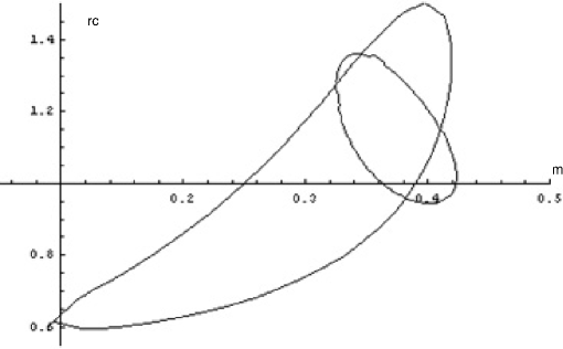
Figure 1: The $1\,\sigma$ confidence region in the $(\Omega_{m}^{0},\Omega_{r_{c}})$-plane from fits to SNeIa data and (i) the constraint (14) (the banana-shaped contour), (ii) the constraint (16)(the elliptic contour)

.

With the approximation $x=1$ the best fit parameter values are

$$\Omega_{m}^{0}=0.26\pm 0.16,~{}\Omega_{r_{c}}=0.82^{+0.69}_{-0.22},~{}\Omega_{A}=2.21^{+0.50}_{-0.22}\,,$$ (15)

with $\chi^{2}=195.5$ for $193-3$ d.f. ($\chi^{2}/d.f.=1.029$), exactly the goodness-of-fit of the $\Lambda$CDM model.

In Fig. 1 we plot the corresponding $1\sigma$ confidence region in the $(\Omega_{m}^{0},\Omega_{r_{c}})$-plane for a $\chi^{2}$ sum including Eqs. (13) and (14), as a banana-shaped contour. Clearly, the weak prior (14) has not done much to remove the degeneracy. The pair of parameters $(\Omega_{r_{c}},\Omega_{A})$ is even more degenerate (not shown here).

Instead of the rather arbitrary prior (14), we include a constraint from the CMB shift parameter $R$, which should not depend crucially on that it has not been derived in five-dimensional brane geometry. $R$ is defined by

$$R(\Omega_{m},\Omega_{r_{c}},\Omega_{A})=\sqrt{\Omega_{m}}H_{0}\int_{0}^{1089}\frac{dz}{xH(z)}~{},$$ (16)

for which the value $R=1.70\pm 0.03$ has been measured [14]. To permit comparison with the banana-shaped contour, we plot the SNeIa fit together with the shift parameter (and with x=1), a nearly elliptically shaped contour, in Fig. 1.

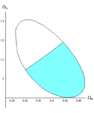
Figure 2: The contour delimits the $1\sigma$ confidence region in the $(\Omega_{m},\Omega_{r_{c}})$-plane in a fit to SNeIa data and the CMB shift parameter. In the blue region the Universe is younger than 12 Gyr.

Fitting next the SNeIa data and $R$ in the same manner as above, but with the correct $x=0.956$, we find

$$\Omega_{m}^{0}=0.40\pm 0.05,~{}\Omega_{r_{c}}=1.1\pm 0.2,~{}\Omega_{A}=2.5\pm 0.3\,,$$ (17)

with $\chi^{2}=195.1$ for $193-3$ d.f. ($\chi^{2}/d.f.=1.027$), slightly better than the fit (15) . We plot in Fig. 2 the corresponding confidence region.

The improvement in $\chi^{2}$ is due to the more exact value of $x$, mostly felt at small redshifts. The exact position of the ellipse is dependent on the value of x, as one can see from comparing the ellipses in Figs. 1 and 2. The shift in the position of the best fit from (15) to (17), is primarily due to the value of the new constraint, the shift parameter $R$.

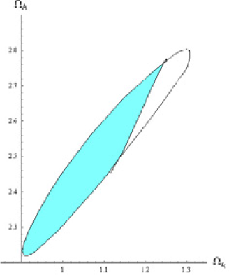
Figure 3: The contour delimits the $1\sigma$ confidence region in the $(\Omega_{r_{c}},\Omega_{A})$-plane in a fit to SNeIa data and the CMB shift parameter. In the blue region the Universe is younger than 12 Gyr.

5 The age of the oldest star

In every theory for a universe expanding with velocity $H(z)$, the age of the universe $t_{U}$ is given by

$$t_{U}=\frac{c}{H(1)}\int_{0}^{1}\frac{da}{H(a)}.$$ (18)

The WMAP collaboration [15] quotes $t_{U}=13.73\pm 0.12$ Gyr from a fit of the $\Lambda$CDM model. In the present model $H(a)$ is given by Eq. (9) with $H(1)=xH_{0}$.

A model-independent limit of $t_{U}$ can be obtained from the age of the oldest star, $t_{\star}$, since $t_{U}>t_{\star}$, and this limit can be used to constrain any model for an expanding universe. Recently, A. Frebel & al. [16] have reported the discovery of HE 1523-0901, a strongly r-process-enhanced metal-poor bright giant star with detected radioactive decay of Th and U. For the first time, it was possible to employ several different chronometers, such as the U/Th, U/Ir, Th/Eu, and Th/Os ratios to measure the age of a star. From 15 such chronometers the weighted average age of HE 1523-0901 is 13.2 Gyr. Leaving out the Th chronometers which have the largest systematic errors, the most useful value is $t_{\star}=13.4\pm 0.8\,(stat)\pm 1.8\,(syst)\,{\rm Gyr}.$ Here the systematic error is mainly due uncertainties in the U production ratio.

The $1\sigma$ statistical error, 0.8 Gyr, can be rewritten as a one-sided 68% confidence limit, $t_{\star}>13.0$ Gyr. The systematic error, 1.8 Gyr, cannot be handled by statistical methods, so we have to resort to a guess. We opt for constraining our model by $t_{U}>12$ Gyr.

The effect of this constraint can be seen in Figs. 2 and 3. In Fig. 2 we over-plot the elliptical contour with the region $t_{U}<12$ Gyr, where the Universe is too young, painted blue. The value of $\Omega_{A}$ along the contour is always the one that minimizes $\chi^{2}$ locally.

In Fig. 3 we plot the $1\sigma$ contour in the $(\Omega_{r_{c}},\Omega_{A})$-plane with the region $t_{U}<12$ Gyr painted blue. The value of $\Omega_{m}$ along the contour is always the one that minimizes $\chi^{2}$ locally. The Universe is too young if the Chaplygin gas acceleration dominates which it does at large values of $\Omega_{A}$, or if the DGP deceleration is too weak which it is at small values of $\Omega_{r_{c}}$.

The value of $\Omega_{m}$ affects $t_{U}$ in the same way as in the standard model: the expansion slows down for increasing values, and the Universe then is younger (blue).

6 Effective dynamics

It is of interest to study the effective dynamics of this model, as expressed by an effective density defined by

$$\rho_{\rm eff}\equiv\rho_{\varphi}-H/\kappa r_{c}\ ,$$ (19)

and an effective equation-of-state parameter

$$w_{\rm eff}\equiv-1-\frac{\dot{\rho}_{\rm eff}}{3H\rho_{\rm eff}}\ .$$ (20)

Inserting $\rho_{\varphi}$ from Eq. (5) and $H$ from Eq. (9) into Eq. (19), one can take time derivatives to obtain $\dot{\rho}_{eff}$ in terms of $\dot{\rho}_{\varphi}$ and $\dot{H}$. The algebraic expressions for $\rho_{eff}$ and $w_{\rm eff}(z)$ are readily calculable when parameter values are inserted, but too long to spell out here.

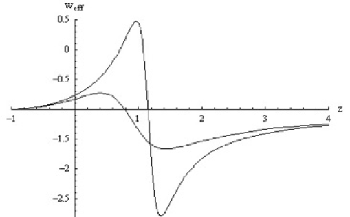
Figure 4: The effective equation-of-state parameter $w_{\rm eff}(z)$ as a function of redshift $z$ at two points within the $1\sigma$ confidence region.

In Fig. 4 we show two curves for $w_{\rm eff}(z)$ corresponding to selected points within the $1\sigma$ confidence range. Both curves are computed at $\Omega_{m}=0.344,~{}\Omega_{A}=2.80$; they differ in the values of $\Omega_{r_{c}}$: 1.07 and 0.90, respectively. At redshifts higher than $z\approx 1$, dark energy exhibits phantom-like acceleration, $w_{\rm eff}<-1$, without phantom matter. In the range $0<z<1$ (depending on the parameter values) dark energy changes from phantom-like acceleration across the phantom divide, $w_{\rm eff}=-1$, to something like quintessence matter, even to $w_{\rm eff}>0$. At the present time one always has $w_{\rm eff}>-1$ inside the $1\sigma$ confidence range of the parameters, and in the future $w_{\rm eff}(z)$ always approaches the cosmological constant value -1.

In most of the parameter space $w_{\rm eff}(z)$ exhibits one or two mathematical singularities, since $\rho_{\rm eff}$ in Eq. (19) clearly can become temporarily negative. The first mathematical singularity develops from the peak and dip near $z=1$ in Fig. 4, and are located where $\rho_{\rm eff}$ changes sign. The second singularity, when present, develops near $z=2$.

Another dynamical quantity of interest is the deceleration parameter $q=-1-\dot{H}/H^{2}$. For redshifts $z\approx 4,~{}q\approx-1.3$, just as at present. In the range $0<z<4,~{}q$ goes through a minimum of $q\approx-1.8$, and in the future it approaches $q=-1$.

7 Discussion and conclusions

We have studied a model combining the 2-parametric self-decelerating DGP model with the likewise 2-parametric standard Chaplygin gas model. The braneworld DGP model is an example of modified gravity which is characterized by a length scale $r_{c}H_{0}$ which marks the cross-over between physics occurring in our four-dimensional brane and in a five-dimensional bulk space. An example of dark energy is Chaplygin gas which has similar asymptotic properties at early and late cosmic times, and a characteristic length scale of its own. We take the two length scales to be proportional, and the proportionality constant subsequently drops out because of a normalizing condition at $a=1$. Our model then depends on only one parameter more than the $\Lambda$CDM model.

The idea to combine the self-decelerating branch of DGP with some accelerating component has been addressed a few times before in the literature. Lue & Starkman [17] and Lazkoz & al. [18] chose the cosmological constant as the accelerating component, mainly in order to explore models with phantom-like acceleration, $w<-1$, for large redshifts, but which approach $w=-1$ in the future. The effective acceleration is then increasing with time as the DGP deceleration vanishes, so that ultimately one recovers the standard cosmological constant model with all its conceptual problems. Since the accelerating component is a constant, it is not characterized by any cross-over scale, nor does this phantom-like acceleration ever cross the phantom divide $w=-1$. Both these papers also discuss observational constraints and possible future signatures.

Models which at large redshifts exhibit phantom-like acceleration, and at small redshifts cross the phantom divide, can also be obtained by replacing the cosmological constant above with a quintessence field (Chimento & al. [19]), or as here and with standard or generalized Chaplygin gas [7] in a decelerated DGP geometry.

It is easy to explain the coincidence problem in the present model as well as in the plain DGP model: it is caused merely by the ratio of the scales of the action, the Planck scale $M_{\rm Pl}$ on our brane and the bulk scale $M_{5}$. These constants happen to have particular time-independent values which determine the DGP cross-over scale $r_{c}$.

We find that the effective EOS is phantom-like at large reshifts, then crosses the phantom divide, so that $w_{\rm eff}(0)>-1$ at the present time. In the future it approaches $w=-1$.

Our model fits SNeIa data with the same goodness-of-fit as the the cosmological constant model, it also fits the shift parameter well, and over a considerable part of the $1\sigma$ confidence range the age of the Universe is more than 14 Gyr, a constraint derived from the age of the star HE 1523-0901. In contrast to most other dark energy models, this model offers a genuine alternative to the cosmological constant model because it does not reduce to it in any limit of the parameter space.

Our model should still be tested against other cosmological data, such as ISW data, CMB and BAO power spectra, all of which has to be derived in a five-dimensional braneworld cosmology. Such a derivation has been done recently [20], so that these constraints can be included in the near future.

References

References

- [1] Dvali, G. R., Gabadadze & Porrati, M., 2000 Phys. Lett. B, 485, 208
- [2] Deffayet, D., 2001 Phys. Lett. B, 502, 199; Deffayet, D, Dvali, G. R. & Gabadadze, 2002 Phys. Rev. D, 65, 044023
- [3] Kamenshchik, A., Moschella, U. & Pasquier, V., 2001 Phys. Lett. B, 511, 265
- [4] Bili, N., Tupper, G. B. & Viollier, R. D., 2002 preprint arXiv: astro-ph/0207423
- [5] Chaplygin, S., 1904 Sci. Mem. Moscow Univ. Math. Phys., 21, 1
- [6] Roos, M., 2007 preprint arXiv: 0704.0882 [astro-ph]
- [7] Bouhmadi-López, M. & Lazkoz, R., 2007 Phys. Lett. B, 654, 51
- [8] Roos, M., 2007 preprint arXiv: 0707.1086 [astro-ph]
- [9] Roos, M., 2007 preprint arXiv: 0804.3297 [astro-ph], to be published in Proc. of the XLIIIst Rencontres de Moriond “Cosmology”, Eds. J. Dumarchez, Y. Giraud-H raud and Jean Trân Thanh Vân, Thê Giói Publishers (2008).
- [10] Davis, T. M. & al., 2007 preprint arXiv: astro-ph/0701510
- [11] Wood-Vasey, W. M. & al., 2007 preprint arXiv: astro-ph/0701041
- [12] Riess, A. G. & al., 2007 Astrophys. J., 659, 98
- [13] Tegmark, M. & al., 2006 Phys. Rev. D74, 123507
- [14] Wang, Y. & Mukherjee, P., 2006 Astrophys. J., 650, 1
- [14] James, F. & Roos, M., 1975 Comput. Phys. Comm., 10, 343
- [15] Hinshaw, G. & al., 2008 preprint arXiv:0803.0732 [astro-ph]
- [16] Frebel, A. & al., 2007 Astrophys. J. Lett., 660, L117
- [17] Lue, A. & Starkman, G. D., 2004 Phys. Rev. D70, 101501(R)
- [18] Lazkoz, R., Maartens, R. & Majerotto, E., 2006 Phys. Rev. D74, 083510
- [19] Chimento, L. P. & al., 2006 J. Cosmol. Astropart. Phys. JCAP09, 004
- [20] Giannantonio, T. & al., 2008 preprint arXiv:0801.4380 [astro-ph]