Strong coupling of light with one-dimensional quantum dot chain: from
Rabi oscillations to Rabi waves

Abstract

Interaction of traveling wave of classic light with 1D-chain of coupled quantum dots (QDs) in strong coupling regime has been theoretically considered. The effect of space propagation of Rabi oscillations in the form of traveling waves and wave packets has been predicted. Physical interpretation of the effect has been given, principles of its experimental observation are discussed.

Introduction. – Rabi oscillations are periodical transitions of a two-state quantum system between its stationary states in the presence of an oscillatory driving field, see e.g. Scully . First observed on nuclear spins in radio-frequency magnetic field Torrey_1949 , the Rabi oscillations then were discovered in many other two-level systems, such as atoms exposed to electromagnetic wave Hocker_Tang_1968 , semiconductor QDs Kamada_2001 , Josephson qubits Blais_07 , spin-qubits Burkard_06 , and between ground and Rydberg atomic states Johnson_08 . Besides the fundamental interest, the effect of Rabi oscillations is promising for realization of binary logic and optical control in quantum informatics and quantum computing.

Complication of physical systems where Rabi effect is observed imposes additional features on the ideal picture Scully of this effect. They are the time-domain modulation of the field-matter coupling constant Law_96 ; yang_04 , the phonon-induced dephasing forstner_03 ; Vagov_07 and the local-field effect Slepyan_04 ; Paspalakis_06 ; Slepyan_07 – just to mention a few. New capabilities appear in systems of two coupled Rabi oscillators Unold_05 ; Gea-Banacloche_06 ; Huges_05 ; Danckwerts_06 ; Ho_Trung_Dung_02 ; Salen_08 ; Tsukanov_06 .

In spatially extensive samples comprising a great number of oscillators, the mechanism giving rise to Rabi oscillations induces also a set of nonstationary coherent optical effects, such as optical nutation, photon echo, self-induced transparency, etc. Shen_84 . This is because the sample size exceeds significantly wavelength and propagation effects come into play. In low-dimensional systems propagation effects are also manifested but their character changes qualitatively. For example, the computational model of the coherent intersubband Rabi oscillations in a sample comprising 80 AlGaAs/GaAs quantum wells Waldmueller_06 predicts the population dynamics to be dependent on the quantum well position in the series. This result demonstrates strong radiative coupling between wells and, more generally, significant difference in the Rabi effect picture for single and multiple oscillators. In the present Letter we build for the first time a theoretical model of a distributed system of coupled Rabi oscillators and predict the new physical effect: the propagation of Rabi oscillations in space in the form of traveling waves and wave packets.

Model and equation of motion. - Consider an interaction of an one-particle excitation in an infinite periodical 1D chain of identical coupled QDs with electromagnetic field. A $p$-th QD is considered as a two-level system with $\left|b_{p}\right\rangle$ and $\left|a_{p}\right\rangle$ as ground and excited states, correspondingly, and the transition frequency $\omega_{0}$. Dephasing and dissipation processes inside the QD are further neglected. The coupling may originate from different physical processes (electron tunneling, dipole-dipole interaction, etc.) and is accounted for in the tight-binding approximation, i.e., is assumed to be restricted to neighboring QDs. Let the QD chain be exposed to a plane wave traveling along the chain, $E\sim\exp[-i(\omega t-kx)]$. The wavenumber satisfies the condition $ka\lesssim 1$ with $a$ as the chain period, providing later on the continuous limit transition.

In the one-particle basis, the Hamiltonian of the system can be represented by $\hat{H}=\hat{H}_{0}+\Delta\hat{H}$, where the term

$$\hat{H}_{0}=\frac{\hbar\omega_{0}}{2}\sum\limits_{n}{\hat{\sigma}_{zn}}-\frac{\hbar\Omega_{R}}{2}\sum\limits_{n}{\hat{\sigma}_{n}^{+}e^{i(nka-\omega t)}+\mathrm{H.c.}}$$ (1)

describes Rabi oscillations in non-interacting QDs. Here, $\hat{\sigma}_{zn}$ and $\hat{\sigma}_{n}^{+}$ are the Pauli matrices for $n$-th QD, and $\Omega_{R}$ is the real-valued Rabi frequency. The term $\Delta\hat{H}$ accounts for the QD-coupling and has the form as follows:

$$\Delta\hat{H}=-\frac{\hbar\xi}{2}\sum\limits_{n}\sum\limits_{p=\pm 1}\left(\left|a_{n}\right\rangle\left\langle a_{n+p}\right|+\left|b_{n}\right\rangle\left\langle b_{n+p}\right|\right)+\mathrm{H.c.},$$ (2)

where $\xi$ is the coupling constant. Equation of motion has the form of one-particle Schrödinger equation $i\hbar\partial_{t}\left|\Psi\right\rangle=\hat{H}\left|\Psi\right\rangle$; the wave function can be written as $\left|{\Psi(t)}\right\rangle=\sum_{p}\left(A_{p}(t)\left|a_{p}\right\rangle+B_{p}(t)\left|b_{p}\right\rangle\right)$. Taking into account (1) and (2), we reduce the Schrödinger equation to a system of differential equations, which directly couples $A_{p}$ with $B_{p},A_{p\pm 1}$ and $B_{p}$ with $A_{p},B_{p\pm 1}$. Carrying out then the continuous limit transition for the variable $A_{p}(t)$ by $A_{p}(t)\rightarrow A(x,t)$, $A_{p+1}(t)+A_{p-1}(t)-2A_{p}(t)\rightarrow a^{2}\partial^{2}_{x}A(x,t)$ and in the same manner for the variable $B_{p}(t)$, in the rotating-wave approximation Scully we arrive at the system of equations as follows:

$$\partial_{t}A=\displaystyle{-\frac{i}{2}(\omega_{0}-4\xi)A+\frac{i\Omega_{R}}{2}Be^{i(kx-\omega t)}+i\xi a^{2}\partial_{x}^{2}A}\,,$$ (3)

$$\rule{0.0pt}{17.22217pt}\partial_{t}B=\displaystyle{\frac{i}{2}(\omega_{0}+4\xi)B+\frac{i\Omega_{R}}{2}Ae^{-i(kx-\omega t)}+i\xi a^{2}\partial_{x}^{2}B}\,,$$ (4)

Eqs. (3) and (4) describe light – QD chain coupling in the framework of formulated model. Because we are interested in the strong coupling regime, the quantity $\Omega_{R}$ can not be considered as a small parameter and further analysis of these equations is carried out without recourse to the perturbation theory.

Traveling Rabi waves. – Let us consider elementary solution of the system (3)–(4) in the form of traveling wave: $A\sim e^{i(h+k/2)x}e^{-i(\nu+\omega/2)t}$, $B\sim e^{i(h-k/2)x}e^{-i(\nu-\omega/2)t}$, where $h$ is a given wave number and $\nu$ is the eigenfrequency to be found. Solving characteristic equation of the system (3)–(4) with respect to $\nu$ determines the eigenfrequencies of system by

$$\nu_{{}_{1,2}}=\xi a^{2}h^{2}-\Phi\pm\left[\Bigl{(}\frac{\Delta}{2}+Vh\Bigr{)}^{2}+\frac{\Omega_{R}^{2}}{4}\right]^{1/2},$$ (5)

where $\Delta=\omega_{0}-\omega$ is the frequency detuning, $V=\xi ka^{2}$ and $\Phi=2\xi(1-k^{2}a^{2}/8)$. These two solutions correspond to two eigenmodes, given, respectively, by

$${\begin{array}[]{l}A_{1}(x,t)=-\displaystyle\frac{C_{1}\Omega_{R}e^{i(h+k/2)x}e^{-i(\nu_{1}+\omega/2)t}}{2(\nu_{1}+\Phi-\Delta/2-Vh-\xi a^{2}h^{2})}\,,\\ \rule{0.0pt}{17.22217pt}B_{1}(x,t)=C_{1}e^{i(h-k/2)x}e^{-i(\nu_{1}-\omega/2)t}\,,\end{array}}$$ (6)

and

$${\begin{array}[]{l}A_{2}(x,t)=C_{2}e^{i(h+k/2)x}e^{-i(\nu_{2}+\omega/2)t}\,,\\ \rule{0.0pt}{25.83325pt}B_{2}(x,t)=-\displaystyle\frac{C_{2}\Omega_{R}e^{i(h-k/2)x}e^{-i(\nu_{2}-\omega/2)t}}{2(\nu_{2}+\Phi+\Delta/2+Vh-\xi a^{2}h^{2})}\,,\end{array}}$$ (7)

where $C_{1,2}$ are normalizing constants. Either of these modes is a superposition of ground and excited states, whose partial amplitudes oscillate both in time and space. Binding of ground and excited states is caused by interaction of light with QD chain and vanishes in the limit of $\Omega_{R}\rightarrow 0$. In that case, Eqs. (6) and (7) describe QD-chain excitons in equilibrium and inverse states, respectively. Retaining in the expansion terms linear in $|\Omega_{R}|$ and simultaneously substituting $\Delta\rightarrow\Delta-i0$ we arrive at the intermediate case of excitons weakly coupled with electromagnetic field.

Space oscillations of the partial amplitudes are due to QD-coupling and vanishes in the limit of $\xi\rightarrow 0$. Thus, each of these modes can be interpreted as a Rabi wave with the frequency determined by Eq. (5). In general case these waves are excited simultaneously, while any of them can be excited separately by a proper choice of initial conditions.

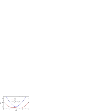
Figure 1: Typical dispersion law for Rabi waves. $\xi=3\Omega_{R}$, $\Delta=0.5\Omega_{R}$, $ka=1$. Turndown of $ha$ corresponds to the range of applicability of the continuous limit model.

Typical dispersion characteristics of Rabi waves are depicted in Fig. 1. It should be noted that at given amplitude and frequency of external field their frequencies have continuous spectra (wave number $h$ varies continuously). Dispersion dependences depicted in the figure are asymmetric: $\nu_{1,2}(h)\neq\nu_{1,2}(-h)$. Physically, this is due to the presence of preferential direction, which is determined by the direction of light propagation along the chain. The QD coupling leads to the inequality $\nu_{1}\neq-\nu_{2}$. That is why, unlike to single QD, in QD chains the inversion oscillates anharmonically. These oscillations can be represented as amplitude-modulated harmonic oscillations with the frequency $(\nu_{1}-\nu_{2})/2$, while the modulation frequency is given by $(\nu_{1}+\nu_{2})/2$. In traveling Rabi wave, the inversion is constant in space. Because $\nu_{1,2}(h)$ are real at any real $h$, the system is stable Landau_Lifshitz_1981 . Now, let us analyse the dispersion characteristics $h_{1,2}(\nu)$, assuming the frequency $\nu$ to be a given parameter. It is seen from Fig.1 that in some frequency range $h_{1}$ is complex and $h_{2}$ is real for real $\nu$. It corresponds to non-transmission of the first Rabi wave Landau_Lifshitz_1981 . The frequency range in which both of $h_{1,2}$ are complex also exists. This case corresponds to complete non-transmission of the Rabi waves with given frequency.

Note that the eigenmodes (6) and (7) each comprise traveling waves with different wave numbers $h\pm k/2$. Physically, this means that the Rabi wave propagates in an effective periodically inhomogeneous medium formed by spatially oscillating (with period $2\pi/k$) electric field. Therefore, the diffraction is developed in the system. In the limit $k\rightarrow 0$ the medium turns homogeneous and the diffraction effect vanishes.

Assuming the frequency $\nu$ to be a given parameter and solving Eq. (5) with respect to wave number, we obtain for $k=0$:

$$h_{1,2}=\pm\left[\frac{1}{a^{2}\xi}\Bigl{(}\nu+2\xi\pm\frac{1}{2}\sqrt{\Omega_{R}^{2}+\Delta^{2}}\,\Bigr{)}\right]^{1/2},$$ (8)

where external signs $\pm$ correspond to two directions of propagation while signs $\pm$ before internal radical correspond to two types of Rabi waves indexed by 1 and 2. It directly follows from (8) that electric field forms an effective medium for propagating Rabi waves. In inhomogeneous electric field the Rabi frequency becomes coordinate-dependent, $\Omega_{R}=\Omega_{R}(x)$, and therefore the medium becomes inhomogeneous too providing reflection of Rabi waves and their mutual transformations at the inhomogeneities. In that way one obtain a unique ability to control the processes of the reflection and dispersion of Rabi waves by varying the light spatial distribution. As a potential realization scheme we indicate the interaction of QD-chain with Gaussian light beam (or superposition of such beams) with the beams’ widths and mutual disposition as controllable factors.

Rabi wave packets. - The process of the excitation transition opens up new opportunities for controlling the dynamics of Rabi oscillations. For identification of control factors we need to know general solution of the system (3)–(4). To find it, we first introduce the variables $u(x,t)=A(x,t)\exp\left[{i}(\omega t-kx-2\Phi t)/{2}\right]$, $v(x,t)=B(x,t)\exp\left[-{i}(\omega t-kx+2\Phi t)/{2}\right]$. For these variables, Eqs. (3)–(4) are reduced to the form as follows:

$$\displaystyle{\partial_{t}u+\frac{i\Delta}{2}u+V\partial_{x}u-i\xi a^{2}\partial^{2}_{x}u-\frac{i\Omega_{R}}{2}v=0\,,}\rule[-14.22636pt]{0.0pt}{2.84526pt}$$ (9)

$$\displaystyle{\partial_{t}v-\frac{i\Delta}{2}v-V\partial_{x}v-i\xi a^{2}\partial^{2}_{x}v-\frac{i\Omega_{R}}{2}u=0\,.}$$

This system can be solved exactly by using the Fourier transform with respect to $x$. Finally we arrive at

$$u(x,t)=\int\limits_{-\infty}^{\infty}\!\!{\left[{\tilde{u}(h)\varphi^{-}_{h}(t)+\tilde{v}(h)\psi_{h}(t)}\right]e^{ih(x-\xi a^{2}ht)}}dh,$$ (10)

$$v(x,t)=\int\limits_{-\infty}^{\infty}\!\!{\left[{\tilde{u}(h)\psi_{h}(t)+\tilde{v}(h)\varphi^{+}_{h}(t)}\right]e^{ih(x-\xi a^{2}ht)}}dh,\,\,$$ (11)

where $\varphi^{\pm}_{h}(t)=\cos\tau\pm i(\Delta_{h}/\Omega_{h})\sin\tau$, $\tau={\Omega_{h}t}/{2}$, $\psi_{h}(t)=i({\Omega_{R}}/{\Omega_{h}})\sin\tau$, $\Omega_{h}=\sqrt{\Omega_{R}^{2}+\Delta_{h}^{2}}$, $\Delta_{h}=\Delta+2Vh$ . The function $\tilde{u}(h)$ is determined by the initial condition

$$\tilde{u}(h)=\frac{1}{2\pi}\int\limits_{-\infty}^{\infty}{u(x,0)e^{-ihx}}dx$$ (12)

and the function $\tilde{v}(h)$ – analogously. It is easy to verify, that the solution obtained satisfies the probability conservation law $\int_{-\infty}^{\infty}[|u(x,t)|^{2}+|v(x,t)|^{2}]\,d\,x=1$ for any $t>0$. A typical space-time distribution of the spatial density of the inversion (the inversion per single QD) $w(x,t)=a[|u(x,t)|^{2}-|v(x,t)|^{2}]$ is shown in Fig. 2a. As follows from Eqs. (10)-(11) the depicted space-time dynamics of $w(x,t)$ corresponds to the evolution of a Rabi wavepacket defined as a superposition of Rabi waves with continuous spectrum of $\Omega_{h}$. Physical interpretation of the picture predicted to observe in the QD chain can be given on base of the collapse-revivals concept Scully . Distinctive feature of the case considered is that the distribution of collapses and revivals is permanently varied in space and time.

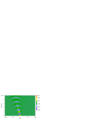
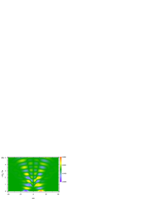
Figure 2: Space-time distribution of the inversion in the QD chain (color online). a) A single Gaussian wavepacket $A(x,0)=\exp(-x^{2}/2\sigma^{2})/\sqrt[4]{\pi\sigma^{2}}$, $B(x,0)=0$, $\Delta=Vk$. b) Two counterpropagating identical Gaussian wavepackets: $A(x,0)=\exp[-(x-3\sigma)^{2}/2\sigma^{2}]/\sqrt[4]{4\pi\sigma^{2}}$, $B(x,0)=\exp[-(x+3\sigma)^{2}/2\sigma^{2}]/\sqrt[4]{4\pi\sigma^{2}}$, $\Delta=0$. In both cases $ka=0.33$, $\sigma=5a$, $\xi=3\Omega_{R}$.

Although variation of the inversion density, depicted in Fig. 2, in arbitrary point of the space occupied by the Rabi wavepacket is not too large, an integral characteristics presented in Fig. 3 – the ”integral” inversion $\int_{-\infty}^{\infty}w(x,t)dx$ – of initially unpolarized QD-chain oscillates between -1 and 1, thus indicating presence of strong light-QD coupling.

Note that oscillations of the integral inversion at $V\neq 0$ damp with time (see Fig. 3), whereas such a damping is absent at $V=0$ and integral inversion oscillates harmonically in the range from -1 to 1 (dotted curve in Fig. 3). Such a behaviour indicates appearance of a specific mechanism of collective dephasing. Physically, this is because the effective detuning $\Delta_{h}$ and therefore the carrier frequency $\Omega_{h}$ of Rabi oscillations constituting the wavepacket depends on $h$ (Doppler shift). As different from that, the condition $V=0$ keeps the $h$-dependence only in the amplitude modulation frequency $(\nu_{1}+\nu_{2})/2$ and thus does not result in dephasing. In the weak coupling limit the indicated dephasing mechanism is analogous to the Landau damping in plasma.

The dependence of the frequency of Rabi oscillations $\Omega_{h}$ on $V$ shows that the value $\Delta=0$ is not optimal for the effect observation. Optimization of $\Delta$ allows increasing the intensity of Rabi wave and the dephasing time, see dashed curve in Fig. 3. In the frequency domain, fine tuning of the system to the resonance is achieved by the variation of $V$ (changing the angle of incidence of light).

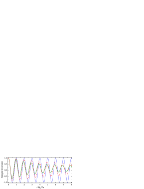
Figure 3: Temporal dependence of the integral inversion at the i put parameters as follows: $\Delta=0$, $k=0$ (dotted line); $\Delta=0$, $ka=0.33$ (solid line); $\Delta=Vk$, $ka=0.33$ (dashed line). In all cases, $\xi=3\Omega_{R}$ and $\sigma=5a$.

Interaction of two counterpropagating identical Gaussian Rabi wavepackets elastically colliding at $x=0$ is shown in Fig. 2b. Although the inversion oscillates in time and moves in space, integral inversion of initially saturated QD chain ($\int_{-\infty}^{\infty}w(x,0)dx=0$) does not experience oscillations: this quantity equals zero for all $t\geq 0$ and arbitrary values of $\Omega_{R}$.

On experimental observability of Rabi waves. - The theory presented can be extended to a various physical situations, such as quantum dynamics of an electron in QD chain. Rabi waves are realized via optically induced transitions between the size-quantized electron levels. Transition of electron from one QD into another occurs by means of tunneling through the potential barrier ref02 ; Tsukanov_06 . Another example is the Rabi oscillations of two-electron entangled state $(|01\rangle+|10\rangle)/\sqrt{2}$ taking place in two neighboring QDs due to dipole-dipole interaction Unold_05 ; Gea-Banacloche_06 ; Huges_05 ; Danckwerts_06 ; Ho_Trung_Dung_02 ; Salen_08 . The model developed describes the motion of this two-electron state as a single whole; in this case the wavefunction $\left|\Psi\right\rangle$ is the envelope function.

Theoretical analysis carried out has shown that the optimal excitation of Rabi waves require the coupling factors of both neighboring QDs and single QD with field to be comparable by magnitude: $\xi\sim\Omega_{R}$. Another necessary condition being imposed on the Rabi frequency is essential exceeding over all intrinsic relaxation rates. For typical QD structures Kamada_2001 , this condition is satisfied for Rabi frequency varied over a wide range $\hbar\Omega_{R}\sim 0.001-1$ meV. This range corresponds to realistic electric field variation $E\sim 10^{2}-10^{5}$ V/cm. As a consequence, the interdot coupling constant $\xi$ also varies between 1 $\mu$eV and 1 meV what is practically achievable Unold_05 ; Tsukanov_06 ; Danckwerts_06 for typical interdot distances $4-20$ nm.

Experimentally, the Rabi waves can be detected in resonant fluorescence spectra of spatially extensive samples by the presence of new spectral lines, additional to the Mollow triplet, as well as by the Doppler shift and broadening of the triplet lines, etc. Of course, highly ordered chains of uniform QDs are required to exclude nonhomogeneous broadening, which may hide the effect. Impressive progress in growing of perfect nanostructured successions achieved in last years (e.g., see Mano ) is very promising for that aim.

Rabi waves can be observed in systems of another physical nature such as quantum electrical circuits Blais_07 , if one proceed from two coupled Josephson cubits in microstrip resonator Blais_07 to a distributed structure of such elements imposed to interqubit interaction. In particular, in that structure the Rabi wave frequency goes down to microwaves and the field intensity necessary for Rabi waves excitation decreases.

Conclusion. - In this Letter, we have predicted the exitance of Rabi waves – wave propagation of the inversion in spatially extensive systems of coupled oscillators. The system has been exemplified by an 1D-chain of coupled QDs exposed to an intensive traveling light wave. Spatial propagation of Rabi oscillations in the form of traveling waves and wave packets is shown to occur in the chain. The propagation is predicted to be accompanied by the damping of Rabi wave in time manifesting new mechanism of collective dephasing, which is an analog of Landau damping of exciton-polaritons extended to the strong light-matter coupling.

Authors acknowledge a support from the INTAS (grant 05-1000008-7801). The work of S.A.M. was partially carried out during the stay at the Institut für Festkörperphysik, TU Berlin, and supported by the Deutsche Forschungsgemeinschaft (DFG). Authors are grateful to Dr. J. Haverkort for stimulative discussions.

References

- (1) M. O. Scully and M. S. Zubairy, Quantum Optics (University Press, Cambridge, 2001).
- (2) H. C. Torrey, Phys.Rev. 76, 1059 (1949).
- (3) G. B. Hocker, C. L. Tang, Phys. Rev. Lett. 21, 591 (1968).
- (4) H. Kamada, H. Gotoh, J. Temmyo, T. Takagahara, and H. Ando, Phys. Rev. Lett. 87, 246401 (2001).
- (5) A. Blais, J. Gambetta, A. Wallraff, D. I. Schuster, S. M. Girvin, M. H. Devoret, and R. J. Schoelkopf, Phys. Rev. A 75, 032329 (2007).
- (6) G. Burkard and A. Imamoglu, Phys. Rev. B 74, 041307(R) (2006).
- (7) T. A. Johnson, E. Urban, T. Henage, L. Isenhower, D. D. Yavuz, T. G. Walker, and M. Saffman, Phys. Rev. Lett. 100, 113003 (2008)
- (8) C. K. Law and J. H. Eberly, Phys. Rev. Lett. 76, 1055 (1996).
- (9) Y. Yang, J. Xu, G. Li and, H.Chen, Phys. Rev. A 69, 053406 (2004).
- (10) J. Förstner, C. Weber, J. Danckwerts, and A. Knorr, Phys. Rev. Lett. 91, 127401 (2003).
- (11) A. Vagov, M. D. Croitoru, V. M. Axt, T. Kuhn, and F. M. Peeters, Phys. Rev. Lett. 98, 227403 (2007).
- (12) G. Ya. Slepyan, A. Magyarov, S. A. Maksimenko, A. Hoffmann, and D. Bimberg, Phys. Rev. B 70, 045320 (2004).
- (13) E. Paspalakis, A. Kalini, and A. F. Terzis, Phys. Rev. B 73, 073305 (2006).
- (14) G. Ya. Slepyan, A. Magyarov, S. A. Maksimenko, and A. Hoffmann, Phys. Rev. B 76, 195328 (2007).
- (15) Th. Unold, K. Mueller, C. Lienau, Th. Elsaesser, and A. D. Wieck, Phys. Rev. Lett. 94, 137404 (2005).
- (16) J. Gea-Banacloche, M. Mumba, and M. Xiao, Phys. Rev. B74, 165330(2006).
- (17) S. Hughes, Phys. Rev. Lett. 94, 227402 (2005).
- (18) J. Danckwerts, K. J. Ahn, J. Förstner, and A. Knorr, Phys. Rev. B73, 165318 (2006).
- (19) Ho Trung Dung, L. Knöll, and D.-G. Welsch, Phys. Rev. A 66, 063810 (2002).
- (20) L. Sælen, R. Nepstad, I. Degani, and J. P. Hansen, Phys. Rev. Lett. 100, 046805 (2008).
- (21) A.V. Tsukanov, Phys. Rev. B73, 085308 (2006).
- (22) Y.R. Shen, The Principles of Nonlinear Optics (John Wiley & Sons, New York, 1984).
- (23) I. Waldmueller, W. W. Chow, and A. Knorr, Phys. Rev. B. 73, 035433 (2006).
- (24) L. D. Landau and E. M. Lifshitz, Physical Kinetics, Course of Theoretical Physics Vol. 10 (Pergamon, Oxford, 1981).
- (25) The tunnel transparency of the barrier is not always identical for both states. As this occurs, the coefficients at and in (2) turn out to be different. The theory developed can easily be extended to this case. Corresponding calculations does not show substantial change of the Rabi waves dynamics comparing with that presented in Fig.2a.
- (26) T. Mano, R. Nötzel, D. Zhou, G. J. Hamhuis, T. J. Eijkemans, and J. H. Wolter, Journal of Appl.Phys. 97, 014304 (2005).