Reliability of regulatory networks and its evolution

Abstract

The problem of reliability of the dynamics in biological regulatory networks is studied in the framework of a generalized Boolean network model with continuous timing and noise. Using well-known artificial genetic networks such as the repressilator, we discuss concepts of reliability of rhythmic attractors. In a simple evolution process we investigate how overall network structure affects the reliability of the dynamics. In the course of the evolution, networks are selected for reliable dynamics. We find that most networks can be easily evolved towards reliable functioning while preserving the original function.

I Introduction

Biological systems are composed of molecular components and the interactions between these components are of an intrinsically stochastic nature. At the same time, living cells perform their tasks reliably, which leads to the question how reliability of a regulatory system can be ensured despite the omnipresent molecular fluctuations in its biochemical interactions.

Previously, this question has been investigated mainly on the single gene or molecule species level. In particular, different mechanisms of noise attenuation and control have been explored, such as the relation of gene activity changes, transcription and translation efficiency, or gene redundancy Ozbudak et al. (2002); Raser and O’Shea (2005); McAdams and Arkin (1999). Apart from these mechanisms acting on the level of the individual biochemical reactions, also features of the circuitry of the reaction networks can be identified which aid robust functioning Barkai and Leibler (1997); Alon et al. (1999); von Dassow et al. (2000). A prime example of such a qualitative feature that leads to an increased stability of a gene’s expression level despite fluctuations of the reactants is negative autoregulation Becskei and Serrano (2000). At a higher level of organization, the specifics of the linking patterns among groups of genes or proteins can also contribute to the overall robustness. In comparative computational studies of several different organisms, it has been shown that among those topologies that produce the desired functional behavior only a small number also displays high robustness against parameter variations. Indeed, the experimentally observed networks rank high among these robust topologies Kollmann et al. (2005); Wagner (2005a); Ma et al. (2006).

However, these models are based on the deterministic dynamics of differential equations. Modeling of the intrinsic noise associated with the various processes in the network requires an inherently stochastic modeling framework, such as stochastic differential equations or a Master equation approach Thattai and van Oudenaarden (2001); Kepler and Elston (2001); Ozbudak et al. (2002); Rao et al. (2002). These complex modeling schemes need a large number of parameters such as binding constants and reaction rates and can only be conducted for well-known systems or simple engineered circuits. For generic investigations of such systems, coarse-grained modeling schemes have been devised that focus on network features instead of the specifics of the reactions involved Bornholdt (2005).

To incorporate the effects of molecular fluctuations into discrete models, a commonly used approach is to allow random flips of the node states. Several biological networks have been investigated in this framework and a robust functioning of the core topologies has been identified Albert and Othmer (2003); Li et al. (2004); Davidich and Bornholdt (2008). However, for biological systems, the perturbation by node state flips appears to be a quite harsh form of noise: In real organisms, concentrations and timings fluctuate, while the qualitative state of a gene is often quite stable. A more realistic form of fluctuations than macroscopic (state flip) noise should allow for microscopic fluctuations. This can be implemented in terms of fluctuating timing of switching events Klemm and Bornholdt (2005a); Chaves et al. (2005); Braunewell and Bornholdt (2007a). The principle idea is to allow for fluctuations of event times and test whether the dynamical behavior of a given network stays ordered despite these fluctuations.

In this work we want to focus on the reliability criterion that has been used to show the robustness of the yeast cell-cycle dynamics against timing perturbations Braunewell and Bornholdt (2007a) and investigate the interplay of topological structure and dynamical robustness. Using small genetic circuits we explore the concept of reliability and discuss design principles of reliable networks.

However, biological networks have not been engineered with these principles in mind, but instead have emerged from evolutionary procedures. We want to investigate whether an evolutionary procedure can account for reliability of network dynamics. A number of studies has focused on the question of evolution towards robustness Wagner (1996); Bornholdt and Sneppen (2000); Ciliberti et al. (2007); Szejka and Drossel (2007); Aldana et al. (2007). However, the evolution of reliability against timing fluctuations has not been investigated. First indications that network architecture can be evolved to display reliable dynamics despite fluctuating transmission times has been obtained in a first study in Braunewell and Bornholdt (2007b). Using a deterministic criterion for reliable functioning, introduced in Klemm and Bornholdt (2005b), it was found that small networks can be rapidly evolved towards fully reliable attractor landscapes. Also, if a given (unreliable) attractor is chosen as the “correct” system behavior, it was shown that with a high probability a simple network evolution is able to find a network that reproduces this attractor reliably, i.e. in the presence of noise.

Here, we want to use a more biologically plausible definition of timing noise to investigate whether a network evolution procedure can generate robust networks. We focus on the question whether a predefined network behavior can be implemented in a reliable way, just utilizing mutations of the network structure. We use a simple dynamical rule to obtain the genes’ activity states, such that the dynamical behavior of the system is completely determined by the wiring of the network.

II Model description

II.1 Boolean dynamics

A widely accepted computational description of molecular biological systems uses chemical master equations and simulation of trajectories by explicit stochastic modeling, e.g. through the Gillespie algorithm Gillespie (1977). However, this method needs a large number of parameters to completely describe the system dynamics. Thus, for gaining qualititative insights into the dynamics of genetic regulatory system it has proven useful to apply strongly coarse-grained models Bornholdt (2005).

Boolean networks, first introduced by Kauffman Kauffman (1969) have emerged as a successful tool for qualitative dynamical modeling and have been successfully employed in models of regulatory circuits in various organisms such as D. melanogaster Albert and Othmer (2003), S. cerevisiae Li et al. (2004), A. thaliana Espinosa-Soto et al. (2004), and recently S. pombe Davidich and Bornholdt (2008).

In this class of dynamical models, genes, proteins and mRNA are modeled as discrete switches which assume one of only two possible states. Here, the active state represents a gene being transcribed or molecular concentrations (of mRNA or proteins) above a certain threshold level. Thus, at this level, a regulatory network is modeled as a simple network of switches.

Time is modeled in discrete steps and the state of all nodes is updated at the same time depending only on the state of all nodes at the previous time step according to the wiring of the network and the given Boolean function.

When such a system is initialized with some given set of node states, it will in general follow a series of state changes until it reaches a configuration that has been visited before (finite number of states). Because of the deterministic nature of the dynamics, the system has then entered a limit cycle and repeats the same sequence of states indefinitely (or keeps the same state in the case of a fixed point attractor).

II.2 Stochastic dynamics

In the original Boolean model there are two assumptions that are clearly non-biological and are thus often criticized: the discrete time which implies total synchrony of all components; and the binary node states which prohibit intermediate levels and gradual effects.

There have been various attempts at loosening these assumptions while keeping the simplicity of the Boolean models. It is a clear advantage of Boolean models that they operate on a finite state space. The synchronous timing, however, does not hold a similar advantage apart from computational simplicity. Models that overcome this synchronous updating scheme have been suggested in a variety of forms. In Chaves et al. (2006) different asynchronous schemes are used in the model of the fruit fly. The simplest asynchronous model keeps the discrete notion of time but lets events happen sequentially instead of simultaneously. A continuous-time generalization of Boolean models that is inspired by differential equation models has been suggested in Klemm and Bornholdt (2005a). Here, the discreteness of the node states is kept but the dynamics take place in a continuous time. In Klemm and Bornholdt (2005b); Braunewell and Bornholdt (2007b) the limit of infinitesimally small disturbances from synchronous behavior is investigated.

This concept of allowing variations from the synchronous behavior will also be used in this work. The principle idea is to use a continuous time description and identify the state of the nodes at certain times with the discrete time steps of the synchronous description Glass (1975). Further, an internal continuous variable is introduced for every node and the binary value of the node is obtained from this continuous variable using a threshold function. Now a differential equation can be formulated for the continuous variable.

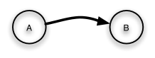
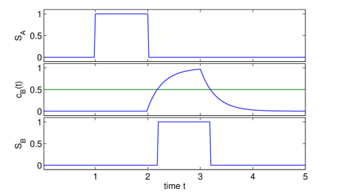
Figure 1: Concentration buildup and decay of a protein given a specific input signal $S_{A}$ and the corresponding activity state $S_{B}$ ($t_{d}=1$, $\tau=0.3$).

This is pictured in figure 1. Here the internal dynamics and the resulting activity state of a node with just one input are shown for a given input pattern. The activator $A$ of the node $B$ is switched on (say, externally) at time $t=1$ and stays on until it is switched off at time $t=2$. In the Boolean description we would say node $A$ assumes state $S_{A}=1$ at time step 1 and at time step 2 switches to state $S_{A}=0$. Node $B$ would react by switching to state $S_{B}=1$ at step 2 and to $S_{B}=0$ at step $3$. In the continuous version, we implement this by a delay time and a “charging” behavior of the concentration value of node $B$, driven by the input variable $S_{A}$. As soon as $c_{B}$ crosses the threshold of $1/2$, the activity state of $B$ switches to $S_{B}=1$.

Let us formulate the time evolution of a system of such model genes by the set of delay differential equations

$$\tau\frac{dc_{i}(t)}{dt}=f_{i}(t,t_{d})-c_{i}(t).$$ (1)

Here, $f_{i}(t,t_{d})$ denotes the transmission function of node $i$ and describes the effect of all inputs of node $i$ at the current time. The parameter $\tau$ sets the time scale of the production or decay process. In general, any Boolean functions can be used as transmission function $f_{i}$. For simplicity, we choose threshold functions, which have proven useful for the modeling of real regulatory networks Li et al. (2004); Davidich and Bornholdt (2008).

Let us use the following transmission function

$$f_{i}(t,t_{d})=\left\{\begin{array}[]{lll}1,&\sum_{j}a_{ij}S_{j}(t-t_{d})\geq T_{i},\\ 0,&\sum_{j}a_{ij}S_{j}(t-t_{d})<T_{i}.\end{array}\right.$$ (2)

where $t_{d}$ is the transmission delay time that comprises the time taken by processes such as translation or diffusion that cause the concentration buildup of one protein to not immediately affect other proteins. The interaction weight $a_{ij}$ determines the effect that protein $j$ has on protein $i$. An activating interaction is described by $a_{ij}=1$, inhibition by $a_{ij}=-1$. If the presence of protein $j$ does not affect expression of protein $i$, $a_{ij}=0$. The discrete state variable $S_{i}$ is determined by the continuous concentration variable $c_{i}$ via a Heaviside function $S_{i}(t)=\Theta[c(t)-1/2]$. The threshold value $T_{i}$ is given by $T_{i}=\sum_{j}a_{ij}/2$ (this choice is equivalent to the commonly used threshold value of 0 if the activity states are given by $S_{i}=\pm 1$ instead of the Boolean values used here).

For the simple transmission function given above, equation (1) can be easily solved piecewise (for every time span of constant transmission function), leading to the following buildup or decay behavior of the concentration levels

$$c_{i}(t>t_{0})=\left\{\begin{array}[]{ll}1-(1-c(t_{0}))\exp(-(t-t_{0})/\tau)&f_{i}\geq 0,\\ c(t_{0})\exp(-(t-t_{0})/\tau)&f_{i}<0.\end{array}\right.$$ (3)

This has the effect of a low-pass filter, i.e. a signal has to sustain for a while to affect the discrete activity state. A signal spike, on the other hand, will be filtered out.

Up to now we have only introduced a continuous, but still deterministic generalization of the synchronous Boolean model. If one now allows noise on the timing delay, the model becomes stochastic and asynchronous. The way we model this stochastic timing is via a signal mechanism. As soon as one node flips its discrete state at, say, $t=t_{0}$, it sends a signal to each node it regulates. This signal affects the input of a regulated node at a later time $t=t_{0}+t_{d}+\chi$ where $\chi$ is a uniformly distributed random number between $0$ and $\chi_{\mathrm{max}}$. The random number $\chi$ is chosen for each signal and each link independently, which means that a switching node will affect two regulated nodes at slightly different times.

Due to the timing perturbations, the network states at exactly integer time do not hold a special significance any more. To overcome this problem, we define a new macro step whenever all discrete node states (not the concentration levels) are constant for at least a time span of $t_{d}/2+\tau$, which amounts to one discrete time step in the synchronous model. Only the system states at these times of extended rest are used in the comparison with the synchronous behavior.

This way, small fluctuations of the signal events are tolerated, but extended times of inactivity of the system must exist and the state of the network at these times must correspond to the respective states under synchronous dynamics. We call network dynamics “reliable” if, despite the stochastic effects on the signal transmission times, the network follows the synchronous state sequence. Although fluctuations in the exact timing are omnipresent, ordered behavior of the sequence of states can still be realized. An exact definition of the algorithm can be found in the appendix.

In Klemm and Bornholdt (2005b) a similar model, but with infinitesimal timing perturbations, was used to identify those attractors in Random Boolean Networks that are reliable. Most attractors in fact are unreliable, but are irrelevant for the system because of very small basins of attraction. Further, it was shown that the number of reliable attractors scales sublinearly with system size, which reconciles the behavior of Boolean dynamics with the numbers of observed cell types as was originally proposed in Kauffman (1993). A similar result was also obtained in a sequential updating scheme Greil and Drossel (2005).

III Reliable and unreliable network dynamics

III.1 Dynamical sequence does not uniquely determine reliability

Figure 2: Comparison of two networks that have a common synchronous attractor. The mutually activating network is unreliable when subject to noise on the signal delay times. In contrast, a negatively autoregulated gene that activates the second exhibits reliable dynamics.

In this section we want to discuss the principle differences behind reliable and unreliable dynamics and show that the same dynamical sequence can be achieved both in a reliable or in an unreliable fashion, depending on the underlying network that drives the dynamics.

We start with the well-known example of two mutually activating genes and model the system according to equations (1) – (3). Apart from the trivial fixed points (both on or both off) this system displays an unreliable attractor as shown in the left panel of figure 2. In the upper part, the synchronous Boolean attractor is depicted in a simple pictorial form (black means active, white inactive). Below that the continuous variable of both nodes is plotted over time in an example run and it can be seen that because of desynchronization the system can exit the synchronous state sequence.

Changing just one link and thus creating an inhibiting self-interaction at the first gene (see right panel of figure 2), the dynamics is now driven by this one node loop. The synchronous sequence of the attractor is still the same, but now the fixed points of the old network are no longer fixed points but transient states to this attractor. The asynchronous dynamics, as shown in the lower part of figure 2 now display an ordered behavior that would continue indefinitely.

The essential feature that causes these stable oscillations is the time delay involved. Without a time delay, the system would not exhibit stable oscillations in either case but would assume intermediate levels for both nodes. Thus, a direct comparison of these dynamics with a stability analysis of ordinary differential equations without delay is not adequate.

III.2 Biological examples

Next, we now want to test the reliability of examples of circuits that can be created artificially. The repressilator is a simple artificially generated genetic circuit implemented in E. coli Elowitz and Leibler (2000). Consisting of of three genes inhibiting each other in a ring topology (see upper part of figure 3), this system displays stable oscillations.

Describing this system using differential equations it was found that the unique steady state is unstable for certain parameter values and that numerical integration of the differential equations displays oscillatory behavior. Also in a stochastic modeling scheme, sustained but irregular oscillations can be observed, which show some resemblance of the experimental time series Elowitz and Leibler (2000).

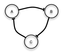
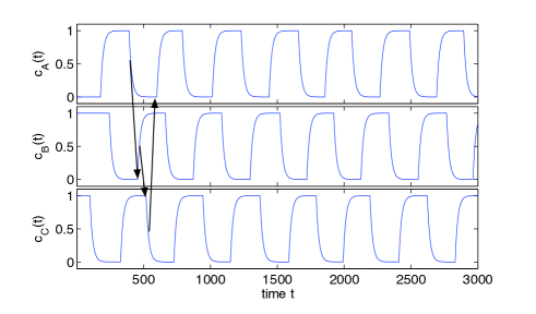
Figure 3: Wiring diagram (top) and example time evolution of concentrations of all three internal variables of the three-gene repressilator. The dynamics is governed by a single event running around the circle – here depicted by arrows which denote the flow of signals.

To discuss this model system in our framework, the synchronous Boolean description has to be analyzed first. Here, the three-gene repressilator exhibits two attractors which comprise all eight network states – the “all-active-all-inactive” (two states) and the “signal-is-running-around” pattern (six states). In the asynchronous scheme, independently of the initial conditions, the system reaches the second attractor. Once the attractor is reached, the system stays in it forever (i.e. is reliable in our definition) – see figure 3. This is due to the fact that only a single switching happens at a given time. This is depicted in the lower part of figure 3 by the arrows which are successively active, no two events happening at the same time.

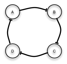
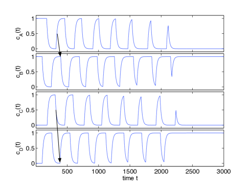
Figure 4: Wiring diagram (top) and example time evolution of concentrations of all four internal variables of the four-gene repressilator. As two events happen independently at the same time (shown by the arrows depicting the signal events), the attractor can be left when the timing of the two event chains desynchronizes.

This picture changes in the case of the four-genes repressilator. The attractor structure is now much more involved, consisting of the two fixed points (1010) and (0101) and three attractors with four states each. Using the stochastic scheme as before, we find that only the fixed points emerge as reliable attractors of the system. If any state of one of the 4-cycles is prepared as initial condition, the system thus always ends up in one of the two fixed points. In figure 4, an example run is shown which is initialized with the state (1100).

Without any noise, the system would follow a four-state sequence consisting of all states where the two active nodes are adjacent and the two inactive nodes are as well. However, if a small perturbation is allowed, the system can exit this attractor as shown in the lower panel of 4. Here, we have drawn two arrows showing two causal events happening at the same time. In fact, there are two independent causal chains in the system dynamics. If these two chains fluctuate in phase relative to each other, they can extinguish each other and drive the system into a fixed point. For an extended discussion of the concept of multiple causal chains, see Klemm and Bornholdt (2005a).

III.3 Stable and unstable dynamics

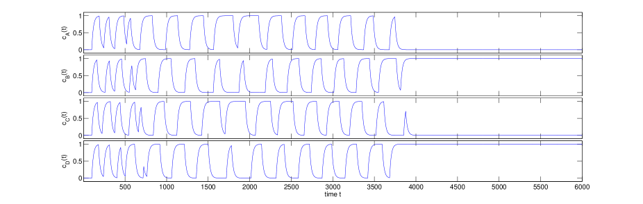
Figure 5: Example of an unstable, a marginally stable and a fixed point attractor in the four-gene repressilator.

Apart from the concept explained in the last section, when a system can accumulate a phase lag through small perturbations in a random walk-like fashion and eventually ends up in a different attractor, there are also examples of systems, in which any small perturbation drives the system away from the current attractor. This is the case if the concentration variables do not reach their maximal value before their input nodes switch their state. This can cause the following node to switch even earlier as compared to the unperturbed timing (in the limit $\tau\to\infty$, this behavior is impossible and each perturbation that is not removed from the system is merely “neutral”).

We show this behavior in figure 5. Here again, the four repressilator is shown, but with the initial state configuration 0000. Without noise, this state belongs to the “all-active-all-inactive” attractor and four independent events are happening at each time step. The small stochastic asynchrony in the beginning is amplified and leads to a quick loss of the attractor. The system then enters an intermediate attractor where the neutral perturbation behavior is predominant, because the concentration levels have more time to approach their saturation value.

The opposite behavior is also possible, that the system itself prevents divergence of the phases. This can happen if the intermediate system state creates a signal spike (i.e. a short-term status change of a node) that itself feeds back to the causal chain. Even though the causal chains are independent in synchronous mode, they can be connected through such intermediate states.

We want to stress that in the criterion employed in Braunewell and Bornholdt (2007b) it cannot be identified whether an attractor is marginally stable or exhibits such a self-catching behavior. This is a limit of the deterministic criterion that is overcome by the explicit modeling used here.

In this work, we consider all attractors as “unreliable” that can desynchronize so strongly that the system does not maintain a “rest phase” in which no switching events occur for an extended time. This includes all marginally stable as well as unstable attractors. We do not distinguish between these in our results as both do not seem suitable for the reliability of a biological system.

IV Network evolution, simulation details

Now that we have introduced the main concepts and ideas surrounding our definition of reliability, we want to turn to the question, whether such a simple model of regulatory networks can be evolved towards realizations displaying reliable dynamics. For this question, we define the notion of a “functional attractor”. As we are dealing with random networks, we need a measure of what the system is supposed to do. Thus, we choose one attractor of the starting network as the prototype dynamics that define the desirable dynamical sequence. The functional attractor is determined by running the synchronous model with a randomly chosen initial state until an attractor is found. During the evolution process we demand each network to reproduce this attractor.

This prescription introduces a bias towards attractors with large basins of attraction. However, as the basin of attraction is commonly understood as a measure of the significance of an attractor, this appears to be a natural choice. Only unreliable attractors are used as functional attractors, as in the case of reliable attractors, the evolution goal would be achieved before the start of the evolution.

The evolution procedure is chosen as a simple version of a mutation and selection process. We start by creating a directed random network with the prescribed number of links $M$ (self-links are allowed) and determine the functional attractor. During the evolution procedure, we mutate the current network by a single rewiring of a link, that is, removal of one link and simultaneous addition of a random link between two nodes that are not yet connected. This actually amounts to two operations on the graph, but has the advantage that the connectivity $\langle k\rangle=M/N$ is kept fixed.

The fitness of a given network is assessed by comparison of the asynchronous dynamics with the synchronous functional attractor. The initial network state is set according to one randomly chosen state of the synchronous attractor. The concentration levels are initialized to the same value (either $0.0$ or $1.0$). Now the system dynamics is explicitly simulated using the stochastic algorithm introduced above (details given in the appendix). We follow the dynamics for maximally $10^{6}$ macro time steps (i.e. rest phases). The fitness score is then obtained by dividing the number of steps correctly following the synchronous behavior by this maximal step number.

The algorithm used in Braunewell and Bornholdt (2007b) is an abstraction of the principle that small fluctuations cannot on its own drive the system out of its attractor, but only if successively adding up. Thus, in a systematic way, for any possible retardation of signal events it is checked whether it persists in the system for a full progression around the attractor. If so, the attractor is marginally stable and can in principle lose its synchrony. While this has the advantage of being a deterministic criterion and thus leads to a noiseless fitness function, there are situations in which this criterion is sufficient but not necessary for reliable behavior. By explicitly modeling the time course, as done in this work, only the truly unstable attractors are marked as such.

We do not take into account the transient behavior of the system and define only the limit cycle as the functional attractor. As our reliability definition would be trivially fulfilled in the case of fixed points, we use networks exhibiting a limit cycle from the start.

In the evolution process, the fitness of a mutant is compared to the fitness that the mother network scored. A network is only selected, if it scores higher than any other network found before during the evolution. As the dynamics is inherently stochastic, the fitness criterion is noisy, too. Thus, networks which are not more reliable than the mother network might still be selected in the evolution due to variability in the fitness score.

If a network follows the attractor up to a maximum step number, it is said to be “reliable”. If during the network process a given number of mutation tries is exceeded, the evolution process is aborted. The maximal number of mutation tries in the evolution is $a_{\mathrm{step}}=20000$ at each step and $a_{\mathrm{tot}}=10^{6}$ during the full course of evolution. We later discuss the implications of these fixed parameter settings.

We have used the following parameters in the results part. The delay time $t_{d}$ is set to unity, the buildup time $\tau$ is $0.1$. Maximal noise $\chi_{\mathrm{max}}$ is $0.02$. This means, that the impact of any individual perturbation is low and cannot itself cause a failure in the fitness test. Only if several perturbations consecutively drive the system away from synchronization, the requirement of an extended static period can be missed.

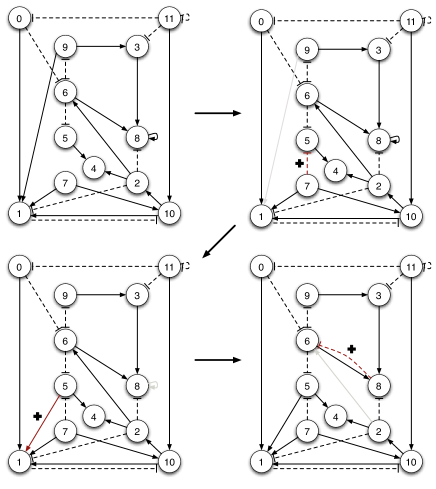
Figure 6: A typical example of an evolution process for a network of size $N=12$. In this example, three steps suffice for stabilization. The structure of each network during the evolution is shown, with the arrows denoting the subsequent step in the evolution. In every step, one link is lost (shown in grey color) and a new link is added (denoted by the plus sign). The change of the state space of the network is given in figure 7.

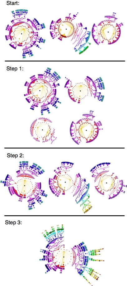
Figure 7: Change of the (synchronous) attractor landscape during evolution – corresponding to the network structures shown in figure 6. For every step, the full attractor landscape is shown. Every dot denotes a state, the subsequent state is connected via a line. The limit cycle is shown in the center of each attractor basin. The functional attractor is shown as the upper leftmost attractor in all steps.

In figures 6 and 7 we show an example of a typical evolution process for a small network of $N=12$. During three steps, the network is evolved towards a reliable architecture. The initial network (upper-left in figure 6) displays three synchronous attractors (top panel in figure 7) of which the first is chosen as the functional attractor. The structural changes are depicted in figure 6 by a grey arrow for the removed link and a plus-sign for the newly added link. As is typical for these evolution processes Braunewell and Bornholdt (2007b), the attractor landscape is affected dramatically during the evolution. In this example, only the functional attractor survives the evolution procedure.

V Results of the network evolution

Figure 8: Ratio of networks that were stabilized during the evolution plotted against the average connectivity of the networks for network sizes of N=16 (straigth line), N=32 (long dashes), N=50 (short dashes).

We have performed the described network evolution for a variety of different network sizes as well as connectivities. For system sizes of $N=16,32$ and $50$ and connectivities between $0.5$ and $6$ the ratio of networks that were stabilized during the evolution is shown in figure 8. Whenever we plot the ratio of stabilized networks, we have calculated the sample errors by a Poissonian error estimate, $\Delta x=\sqrt{x(1-x)/n}$, where $x$ is the obtained ratio from $n$ sample runs.

One can see that for intermediate connectivities between $2.5$ and $4.5$, the ratio of stabilized networks is above 80% for all system sizes under investigation. This means, that starting from any random network, in four out of five cases a simple network evolution is able to find a network that displays the same dynamical attractor, but performs it reliably.

This result matches a very similar dependence on the connectivity that was found for 16 nodes in the infinitesimal scheme in Braunewell and Bornholdt (2007b).

It is interesting to note that for lower connectivities, the ratio of stabilized networks decreases significantly. For all system sizes considered, there is a sizable decrease of the stabilization ratio for connectivities below two. This is especially apparent for the large system size $N=50$. This is due to the “essentiality” of the structure on the dynamics. Changing a link without destroying the dynamical attractor is less likely for lower connectivities. At higher connectivities the larger number of non-essential links in the system aids evolvability towards reliable dynamics via phenotypically neutral mutations.

However, considering large connectivities and large system sizes, the ratio of stabilized networks drops again. along with the increase of attractor lengths with system size that impairs reproducibility of dynamics. Thus, we find an area of connectivity between $1.5$ and $4.5$ for which the ratio of stabilized networks is similar for all system sizes considered.

Figure 9: Average number of evolution steps until stable realization is reached ($N=32$)

The plot in figure 9 shows the average number of rewiring steps necessary until a stable network realization is found for networks of 32 nodes. For all connectivities, this number is remarkably low, as the evolution procedure basically implements a biased random walk through structure space. This is due to the large variation of the fitness score of a single network. Despite the rather small evolutionary pressure, the evolution procedure quickly finds a realization exhibiting reliable dynamics. Interestingly, the number of evolution steps does not monotonically grow with the connectivity, but instead drops for connectivities larger than two.

This again is an indication that networks with higher connectivities are easier to evolve towards reliability. The ratio of links rewired in the evolution to the total number of links is even monotonically decreasing (not shown).

Figure 10: Ratio of networks that were stabilized during the course of evolution plotted against the number of nodes in the networks for an average connectivity of $\langle k\rangle=2$. The dashed line is given by a logarithmic fit of the data.

We want to further investigate the dependence on network size by repeating the evolution procedure with system sizes up to $N=400$. This is shown in figure 10 in a log-linear plot of the ratio of stabilized networks vs. system size. We find that the ability of the process to stabilize a given network decreases with system size. The line in the figure represents a fit of the function $f(N)=a-b\log(x)$ with $a=1.416$, $b=0.198$ thus a relatively slow decay with system size. One also has to keep in mind that the fixed set of parameters for the number of attempted mutations per evolution step and the total number of attempted mutations during the evolution reduces the success rate for larger networks. For small networks of $N=16$, 20000 attempted mutations per evolution step suffices for a good estimate of the space of all one-link mutations, but as the number of possible mutations scales with the system size N as $N^{3}$, it quickly becomes impossible to check all possibilities. Thus, the results in figure 10 underestimate the probability to find a stable instance.

Figure 11: Comparison of parameter values. Ratio of networks that were stabilized against the number of nodes in the networks for an average connectivity of $\langle k\rangle=2$. Original set of parameters marked with ‘$+$’, points obtained with increased step number marked with ‘$\times$’.

Figure 12: Effect of parameter $a_{\mathrm{step}}$ on the results for $N=50$. The ratio of stabilized networks is plotted against the value of the paramter $a_{\mathrm{step}}$, giving the maximal number of attempted mutations per evolution step.

We have checked the dependence of the results on the selection parameters (attempted mutations per evolution step $a_{\mathrm{step}}$ and total number of attempted mutations during evolution $a_{\mathrm{total}}$) for selected network sizes and connectivities. In figure 11 we again show the ratio of stabilized networks against system size, but this time for two different parameter values – the original parameter set with $a_{\mathrm{step}}=2\cdot 10^{4}$ (denoted by ‘+’) and for an increased value of $a_{\mathrm{step}}=10^{5}$ (denoted by ‘$\times$’). For small networks, the value of this parameter does not significantly affect the results, but for $N>50$, differences can be clearly seen. For $N=50$ the ratio rises from $0.65\pm 0.02$ at $a_{\mathrm{step}}=2\cdot 10^{5}$ to $0.72\pm 0.02$ at $a_{\mathrm{step}}=10^{6}$. Interestingly, for larger system sizes this effect does not seem to be amplified: for $N=100$ the ratio rises from $0.51\pm 0.02$ to $0.55\pm 0.02$.

For $N=50$ we plot the dependence of the ratio of stabilized networks on the parameter $a_{\mathrm{step}}$ in figure 12. The largest parameter value used, $a_{\mathrm{step}}=10^{6}$ is about twice the total number of possible rewirings and should thus suffice.

One can see that the decrease in the ratio of successfully evolved networks can be significantly reduced when attempting more mutations per evolution step. This is due to the fact that an enormous number of mutations is possible of which only a small fraction retains the requested dynamical sequence.

Still, one can deduce from these results that it is harder to stabilize large networks than smaller ones: even though there might be a path to a stable network instance, it may not be practically realizable as the chance to find exactly the right mutations may be too small.

However, real world systems display a large amount of modularity that leads to smaller cores of strongly interacting components. We have not taken this into account in our random network approach. We see this as a model for small networks of key generators as were described in recent Boolean models of biological systems Li et al. (2004); Davidich and Bornholdt (2008). The resulting dynamics of the full networks are then influenced by this core without strong feedback. This allows for rather simple expression patterns of the full network without constraints on the network size.

VI Summary and Conclusions

We have discussed a simple reliability criterion for biological networks and have applied it to network design features that produce reliable dynamics. We showed that small changes in the network topology can dramatically affect the dynamical behavior of a system and can lead to reliable network dynamics.

To investigate how reliability can emerge in real-world systems that have been shaped by evolution, we studied an evolutionary algorithm that selects networks with a prescribed dynamical behavior if they function more reliably than a given mother network.

We found that a high ratio of random networks can evolve towards instances displaying reliable dynamics. In accordance with other recent work Szejka and Drossel (2007); Ciliberti et al. (2007), it was shown that the evolution of network structures can lead to reliable dynamics both with a high probability and within short evolutionary time scales.

Surprisingly, small connectivities are detrimental to this evolvability. This is counter-intuitive as sparsely connected networks show rather simple dynamics with short attractor lengths. However, at the same time they are difficult to evolve because they have a small structural “buffer” of links that can be neutrally rewired without changing the dynamics.

This is related to the concepts of “degeneracy” and “distributed robustness” where additional elements are present in a system that are not strictly necessary for the system’s function but have a positive effect on robustness Tononi et al. (1999); Wagner (2005b). Here, these additional elements are links that are not strictly necessary to perform a specific function. Thus, rewiring of these links is possible and allows for a higher probability to find a network with reliable dynamics. We thus find in our framework that high connectivity, although leading to increasing complexity of the dynamics, can be beneficial for the evolution of networks.

For larger system sizes the evolvability towards reliable dynamics decreases. This is due to the increasing dynamical complexity of such networks (longer attractor cycles, more non-frozen nodes). Our strict criterion requests the reliable reproduction of the exact state sequence for every node, which leads to a more difficult selection process for large system sizes.

In summary, our results suggest that reliability is an evolvable trait of regulatory networks. In the present simple model, reliability can be achieved by topological changes alone and without fine-tuning of parameters. This means that through mutations of the reaction networks, biological systems may have the ability to rapidly acquire the property of reliable functioning in the presence of biochemical stochasticity.

Appendix A Algorithm

The asynchronous algorithm is implemented such that no discretized clock is needed. Only those times will be investigated, when changes in the system happen.

For this, internal variables are needed to keep track of the dynamics. Every node $i$ has the following state variables:

• $t_{0,i}$: time of the last change of buildup/decay behavior

• $c_{i}(t_{0,i})$: concentration level at that time

• $b_{i}$: flag for current behavior - either buildup (1) or decay (0)

• $s_{i,\mathrm{current}}$: current discrete state of node $i$

• $s_{i,\mathrm{aim}}$: discrete state of node $i$ that would result from the current states of all nodes: ${s_{i,\mathrm{aim}}=\Theta\left(\sum_{j=1}^{n}a_{ij}s_{j,\mathrm{current}}-1/2\right)}$,

In addition, a global event queue $Q$ is maintained which keeps track of future changes in buildup/decay behavior.

The system is initialized by setting all values of discrete states $s_{i,\mathrm{current}}$ equal to the state given by the discrete initial conditions. The concentration levels are set to the same values ($0.0$ or $1.0$). The times of the last behavior changes $t_{0,i}$ are set to $0$.

Before the simulation is started, for every node $i$ it is checked whether the aspired state $s_{i,\mathrm{aim}}$ differs from the current state $s_{i,\mathrm{current}}$. If so, an event is added to the queue Q (sorted by time) for time $t_{d}+\chi$, where $\chi$ is a uniformly distributed random number between $0$ and $\chi_{\mathrm{max}}$.

When the simulation is run, it is checked which of the two following possible events takes place next:

1. Crossing of the concentration level of a node with the threshold value $0.5$

2. The next event in queue $Q$

A simple analytical expression can be given for the times when the concentration levels are crossed (case 1). If $b_{i}=s_{i,\mathrm{current}}$, the node will not switch its state because the concentration is moving away from the threshold. Otherwise, one can calculate the time of the next concentration level to cross the threshold by solving equation (3) for $t$ with $c_{i}=0.5$:

$$\min_{i}\left[t_{0,i}+\tau\log(1+|1-2c_{i}(t_{0,i})|)\right]$$ (4)

If an event of type 1 happens next, the discrete state of the respective node $i$, $s_{i,\mathrm{current}}$, is updated and the effect on other nodes is calculated. For definiteness, let us assume this crossing takes place at time $t$. If this switch causes the aspired state of another node $j$ to switch, an event is sorted into the queue $Q$ at $t+t_{d}+\chi$. When in the queue events for the same node are scheduled to happen at later times, they will be removed. They are thought to have been “caught” by the newly added event.

In the second case, the concentration level of the node at time $t$ is calculated according to equation (3) and saved as $c_{i}(t_{i,0})$ with the new time $t_{i,0}$. The behavior flag $b_{i}$ is switched to reflect that the node has changed from buildup to decay or vice versa.

If the time between any two successive node state changes in the network (not necessarily of the same node) is larger than $t_{d}/2+\tau$, the node states are recorded and set as a new step to be compared to the synchronous attractor.

References

- Ozbudak et al. (2002) E. M. Ozbudak, M. Thattai, I. Kurtser, A. D. Grossman, and A. van Oudenaarden, Nat Genet 31, 69 (2002), ISSN 1061-4036 (Print).
- Raser and O’Shea (2005) J. M. Raser and E. K. O’Shea, Science 309, 2010 (2005).
- McAdams and Arkin (1999) H. H. McAdams and A. Arkin, Trends Genet 15, 65 (1999).
- Barkai and Leibler (1997) N. Barkai and S. Leibler, Nature 387, 913 (1997).
- Alon et al. (1999) U. Alon, M. G. Surette, N. Barkai, and S. Leibler, Nature 397, 168 (1999).
- von Dassow et al. (2000) G. von Dassow, E. Meir, E. M. Munro, and G. M. Odell, Nature 406, 188 (2000).
- Becskei and Serrano (2000) A. Becskei and L. Serrano, Nature 405, 590 (2000).
- Kollmann et al. (2005) M. Kollmann, L. Lovdok, K. Bartholome, J. Timmer, and V. Sourjik, Nature 438, 504 (2005).
- Wagner (2005a) A. Wagner, Proc. Natl. Acad. Sci. USA 102, 11775 (2005a).
- Ma et al. (2006) W. Ma, L. Lai, Q. Ouyang, and C. Tang, Mol Syst Biol 2, 70 (2006).
- Thattai and van Oudenaarden (2001) M. Thattai and A. van Oudenaarden, Proc. Natl. Acad. Sci. USA 98, 8614 (2001).
- Kepler and Elston (2001) T. B. Kepler and T. C. Elston, Biophys. J. 81, 3116 (2001), eprint http://www.biophysj.org/cgi/reprint/81/6/3116.pdf.
- Rao et al. (2002) C. V. Rao, D. M. Wolf, and A. P. Arkin, Nature 420, 231 (2002).
- Bornholdt (2005) S. Bornholdt, Science 310, 449 (2005).
- Albert and Othmer (2003) R. Albert and H. G. Othmer, J. Theor. Biol. 223 (1), 1 (2003).
- Li et al. (2004) F. Li, T. Long, Y. Lu, Q. Ouyang, and C. Tang, Proc. Natl. Acad. Sci. USA 101(14), 4781 (2004).
- Davidich and Bornholdt (2008) M. I. Davidich and S. Bornholdt, PLoS ONE 3, e1672 (2008), ISSN 1932-6203 (Electronic).
- Klemm and Bornholdt (2005a) K. Klemm and S. Bornholdt, Proc. Natl. Acad. Sci. USA 102, 18414 (2005a).
- Chaves et al. (2005) M. Chaves, R. Albert, and E. D. Sontag, J. Theor. Biol. 235, 431 (2005), ISSN 3.
- Braunewell and Bornholdt (2007a) S. Braunewell and S. Bornholdt, J. Theor. Biol. 245, 638 (2007a).
- Wagner (1996) A. Wagner, Evolution 50, 1008 (1996).
- Bornholdt and Sneppen (2000) S. Bornholdt and K. Sneppen, Proc. R. Soc. Lond. B 267, 2281 (2000).
- Ciliberti et al. (2007) S. Ciliberti, O. C. Martin, and A. Wagner, PLoS Comp. Biol. 3 (2007).
- Szejka and Drossel (2007) A. Szejka and B. Drossel, Eur. Phys. J. B 56, 373 (2007).
- Aldana et al. (2007) M. Aldana, E. Balleza, S. Kauffman, and O. Resendiz, J. Theor. Biol. 245, 433 (2007).
- Braunewell and Bornholdt (2007b) S. Braunewell and S. Bornholdt (2007b), arXiv:0707.1407.
- Klemm and Bornholdt (2005b) K. Klemm and S. Bornholdt, Phys. Rev. E 72, 055101(R) (2005b).
- Gillespie (1977) D. T. Gillespie, J. Phys. Chem. 81, 2340 (1977).
- Kauffman (1969) S. A. Kauffman, J. Theor. Biol. 22, 437 (1969).
- Espinosa-Soto et al. (2004) C. Espinosa-Soto, P. Padilla-Longoria, and E. R. Alvarez-Buylla, Plant Cell 16, 2923 (2004).
- Chaves et al. (2006) M. Chaves, E. D. Sontag, and R. Albert, Systems Biology, IEE Proceedings 153, 154 (2006).
- Glass (1975) L. Glass, J. Phys. Chem. 63, 1325 (1975).
- Kauffman (1993) S. A. Kauffman, The Origins of Order (Oxford University Press, New York, 1993).
- Greil and Drossel (2005) F. Greil and B. Drossel, Phys. Rev. Lett. 95, 048701 (2005).
- Elowitz and Leibler (2000) M. B. Elowitz and S. Leibler, Nature 403, 335 (2000).
- Tononi et al. (1999) G. Tononi, O. Sporns, and G. M. Edelman, Proc. Natl. Acad. Sci. USA 96, 3257 (1999), eprint http://www.pnas.org/cgi/reprint/96/6/3257.pdf.
- Wagner (2005b) A. Wagner, Bioessays 27, 176 (2005b).