Landau levels and Riemann zeros

Abstract

The number $N(E)$ of complex zeros of the Riemann zeta function with positive imaginary part less than $E$ is the sum of a ‘smooth’ function $\bar{N}(E)$ and a ‘fluctuation’. Berry and Keating have shown that the asymptotic expansion of $\bar{N}(E)$ counts states of positive energy less than $E$ in a ‘regularized’ semi-classical model with classical Hamiltonian $H=xp$. For a different regularization, Connes has shown that it counts states ‘missing’ from a continuum. Here we show how the ‘absorption spectrum’ model of Connes emerges as the lowest Landau level limit of a specific quantum mechanical model for a charged particle on a planar surface in an electric potential and uniform magnetic field. We suggest a role for the higher Landau levels in the fluctuation part of $N(E)$.

At the begining of the 20th century Polya and Hilbert conjectured that the imaginary part of the complex zeros of the Riemann zeta function $\zeta(s)$ are the eigenvalues of a self-adjoint operator $H$. The existence of such an operator implies the celebrated Riemann hypothesis that all complex zeros lie on the ‘critical line’ ${\mathcal{R}e}(s)=1/2$. Support for this ‘spectral’ approach did not emerge until the 1950s, when Selberg found a ‘trace’ formula relating the eigenvalues of the Laplacian on a compact hyperbolic surface to its geodesics; there is a strong resemblance of this formula to the Riemann-Weil ‘explicit’ formula relating the Riemann zeros to the prime numbers. Further support came in the 1970s and 80s from the works of Montgomery and Odlyzko: assuming the Riemann hypothesis, they showed that the local statistics of the Riemann zeros is described by the Gaussian Unitary Ensemble (GUE) of Random Matrix Theory (see e.g. Frontiers ). Inspired by this, and by analogies between trace formulas of number theory and the Gutzwiller formula for chaotic dynamical systems, Berry conjectured the existence of a classical chaotic Hamiltonian system with isolated periodic orbits, with periods related to the prime numbers, such that the spectrum of the quantum theory gives the complex Riemann zeros B-chaos . The GUE statistics of the zeros requires the Hamiltonian to break time-reversal invariance.

Berry’s conjecture received support in 1999 from the work of Connes Connes , and Berry and Keating BK1 , on a semi-classical model for a particle in one dimension with classical Hamiltonian $H=xp$. This Hamiltonian breaks time-reversal invariance since $(x,p)\to(x,-p)\Rightarrow H\to-H$. Classical orbits in this model are unbounded hyperpolas in phase space but they may be converted into closed orbits by an identification at the boundaries of a restricted region of the phase plane that defines some ‘regularization’ of the model. This regularization also makes finite the number of states with energy less than $E$, and this number is related to the number $N(E)$ of complex zeros of the Riemann zeta function with positive imaginary part less than $E$. The Riemann-van Mangoldt ‘counting’ formula states that

$$N(E)=\overline{N}(E)+\frac{1}{\pi}{\mathcal{I}m}\,\log\zeta\left(\frac{1}{2}+iE\right)\,$$ (1)

where $\overline{N}(E)$ is a ‘smoothed’ counting function that gives the average number of zeros, which is corrected by the remaining ‘fluctuation’ term. The smooth term can be written as

$$\overline{N}(E)=\frac{\theta(E)}{\pi}+1\,,$$ (2)

where (see e.g. Edwards )

$$\theta(E)={\mathcal{I}m}\,\log\Gamma\left(\frac{1}{4}+i\frac{E}{2}\right)-\frac{E}{2}\log\pi\,,$$ (3)

which is the phase of the zeta function on the critical line. The smooth term has the following asymptotic expansion for large $E$:

$$\overline{N}(E)\sim\frac{E}{2\pi}\log\frac{E}{2\pi}-\frac{E}{2\pi}+{\cal O}(1)\,,$$ (4)

while the fluctuation term is of order $\log E$. In the Berry-Keating model this asymptotic expression for $\overline{N}(E)$ is recovered from a semi-classical count of states with positive energy less than $E$; the correct ${\cal O}(1)$ term is obtained by taking into account the Maslov phase implied by the identifications that close the hyperbolic orbits BK1 . In the Connes model, which has a different ‘regularization’, the same asymptotic expression is found as a semi-classical count of states missing from a continuous spectrum. Thus, the Berry-Keating interpretation of $\overline{N}(E)$ is as an ‘emission’ spectrum while the Connes interpretation is as an ‘absorption’ spectrum.

The first aim of this letter is to show how these semi-classical results can be recovered by viewing the $H=xp$ model as a lowest Landau level (LLL) limit of a quantum mechanical model for a charged particle on the $xy$-plane in a constant uniform perpendicular magnetic field of strength $B$, and an electric potential $\varphi=-\lambda xy$, where $\lambda$ is a constant. Let $\mu$ be the particle’s mass and $-e$ its charge. In the Landau gauge $A=Bxdy$ for the vector potential 1-form $A$, the particle’s Lagrangian is

$${\bf L}=\frac{\mu}{2}(\dot{x}^{2}+\dot{y}^{2})-\;\frac{eB}{c}\;\dot{y}x-e\,\lambda\,xy\,.$$ (5)

This Lagrangian is invariant under $(x,y)\to(-x,-y)$, which implies a double degeneracy of states of energy $E$. It is also quadratic, with two normal modes: the standard ‘cyclotronic’ mode of the $\lambda=0$ model, and a ‘hyperbolic’ mode. The respective angular frequencies are

$$\omega_{c}=\frac{eB}{\mu c}\cosh\vartheta,\,\qquad\omega_{h}=i\frac{eB}{\mu c}\sinh\vartheta\,,$$ (6)

where $\sinh(2\vartheta)=(2\lambda\mu c^{2})/(eB^{2})$; for simplicity, we shall consider the limiting case $\omega_{c}\gg|\omega_{h}|$, for which

$${\omega_{c}}\approx\frac{eB}{\mu c},\qquad{\omega_{h}}\approx i\frac{\lambda c}{B}\,.$$ (7)

In the quantum theory, the energy in the cyclotronic mode is $(n+1/2)\hbar\omega_{c}$ for integer $n$ labelling the Landau level. At sufficiently low energy only the lowest ($n=0$) level is relevant and the physics is effectively described by the Lagrangian (see e.g. Shankar )

$${\bf L}_{LLL}=p\dot{x}-|\omega_{h}|xp\,\qquad p=\frac{\hbar y}{\ell^{2}}\,,\qquad\ell^{2}=\frac{\hbar c}{eB}\,.$$ (8)

where $\ell$ is the ‘magnetic’ length. This LLL model is the (unregularized) one-dimensional $H=xp$ model. From the Landau model perspective, each quantum state is associated to a quantum of magnetic flux $\Phi_{0}=2\pi\hbar c/e$ that occupies an area $2\pi\ell^{2}$ in the $xy$-plane. In the LLL limit, this implies the standard semi-classical quantization in which one quantum state is associated with an area $2\pi\hbar$ in phase space.

The total number of states in each Landau level, in particular the lowest one, is infinite. To make the number of states in each level finite, we shall restrict the particle to the square

$$|x|<L\,,\qquad|y|<L\,.$$ (9)

This implies for the LLL model a restriction on the phase space equivalent to that proposed by Connes for the $H=xp$ model. It also implies that there is a maximum magnitude for the classical energy: $|E|\leq L^{2}/\ell^{2}$ in units for which $\hbar\omega_{h}=1$, which fixes the value of $\lambda$ in terms of $e$ and $B$ by (7). For large $L/\ell$, the semi-classical estimate for the total number of quantum states of any energy allowed by this bound is $L^{2}/2\pi\ell^{2}$ in each of the four quadrants in the $xy$-plane separated by the $x$ and $y$ axes. The classical trajectory for a particle of energy $E<E_{max}$ is the hyperbola $xy=E\ell^{2}$, so the available classical phase space is the region in the square that lies between the two branches of the hyperbola. The number $N_{sc}(E)$ of semi-classical quantum states with energy less than $E$ is the area of this region divided by $2\pi\ell^{2}$, but because of the double-degeneracy due to the $(x,y)\to(-x-y)$ symmetry we count only those states with $(x>0,y>0)$, which yields

$$N_{sc}(E)=\frac{E}{2\pi}\log\frac{L^{2}}{2\pi\ell^{2}}-\frac{E}{2\pi}\log\frac{E}{2\pi}+\frac{E}{2\pi}\,.$$ (10)

The first term diverges as $L\to\infty$ and may be interpreted as a regularization of the continuum of states in the lowest Landau level for a particle free to move on the entire $xy$-plane. The finite correction, which has a magnitude equal to the asymptotic approximation of (4) to the smooth part of the counting formula, is negative, which led Connes to interpret it as representing spectral lines missing from the continuum.

Another aim of this letter is to use the Landau model perspective to arrive at a proper quantum-mechanical understanding of the regularized $H=xp$ model of Connes; we focus on that model (details of which may be found in a recent book CM ) because we have not seen how to achieve the same objective for the Berry-Keating model. The Hamiltonian operator corresponding to the starting Lagrangian (5) is

$$H=\frac{1}{2\mu}[\widehat{p}_{x}^{2}+(\widehat{p}_{y}+\frac{\hbar}{\ell^{2}}x)^{2}]+e\lambda xy\,,$$ (11)

where $\widehat{p}_{x}=-i\hbar\partial_{x}$ and $\widehat{p}_{y}=-i\hbar\partial_{y}$. There is a unitary transformation in which this Hamiltonian becomes the sum of a Hamiltonian $H_{c}$ for the cyclotronic mode and a Hamiltonian $H_{h}$ for the hyperbolic mode. In units for which $\hbar=\ell=1$, one finds that

$$H_{c}=\frac{\omega_{c}}{2}(\widehat{p}^{2}+q^{2})\,,\qquad H_{h}=\frac{|\omega_{h}|}{2}(Q\widehat{P}+\widehat{P}Q)\,,$$ (12)

where $\widehat{P}=-id/dQ$ and $\widehat{p}=-id/dq$. Note the Weyl ordering in $H_{h}$, which follows from the starting Hamiltonian. The unitary transformation that achieves this decomposition simplifies considerably in the limit that $\omega_{c}\gg|\omega_{h}|$; it corresponds to the classical canonical transformation

$$q=x+p_{y}\,,\quad p=p_{x}\,,\quad Q=-p_{y}\,,\quad P=y+p_{x}\,.$$ (13)

In the limit that $\omega_{c}\gg|\omega_{h}|$, any low energy eigenstate is the product of the ground state of $H_{c}$, which is the gaussian $\psi=\exp(-q^{2}/2\ell^{2})$, with an eigenstate of $H_{h}$, which we may choose to be either even or odd under $Q\to-Q$. These eigenstates of definite ‘$Q$-parity’ are

$$\Phi_{E}^{+}(Q)=\frac{1}{|Q|^{1/2-iE}}\,,\qquad\Phi_{E}^{-}(Q)=\frac{{\rm sign}(Q)}{|Q|^{1/2-iE}}\,.$$ (14)

The corresponding wavefunctions of the original Hamiltonian are then given by

$$\psi^{\pm}_{E}(x,y)=C\int dQ\,e^{-iQy/\ell^{2}}\;e^{-(x-Q)^{2}/2\ell^{2}}\,\Phi^{\pm}_{E}(Q)\,.$$ (15)

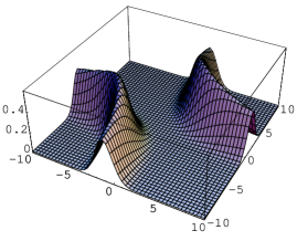
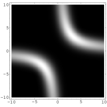
where $C$ is a normalization constant. This yields

$$\psi^{+}_{E}(x,y) = C^{+}_{E}e^{-\frac{x^{2}}{2\ell^{2}}}\,M\left(\frac{1}{4}+\frac{iE}{2},\frac{1}{2},\frac{(x-iy)^{2}}{2\ell^{2}}\right)$$ (16)

$$\psi^{-}_{E}(x,y) = C^{-}_{E}(x-iy)e^{-\frac{x^{2}}{2\ell^{2}}}\,M\left(\frac{3}{4}+\frac{iE}{2},\frac{3}{2},\frac{(x-iy)^{2}}{2\ell^{2}}\right)$$

where $M(a,b,z)\equiv{}_{1}F_{1}(a,b,z)$ is a confluent hypergeometric function. A representative plot of the even wavefunction is shown in Fig.1.

Figure 1: Absolute value of the wave function $\psi^{+}_{E}(x,y)$ for $E=10$ in the interval $-10<x,y<10$. The picture on the left gives a 3D representation while that on the right is a density plot.

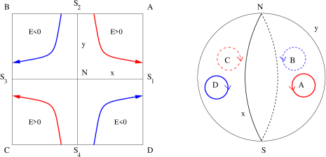
A classical trajectory that starts at $(x,L)$ ends at $(L,x)$, so that identification of these points creates periodic orbits. This identification also means that the square in the $xy$-plane in which the particle is allowed to move is topologically a sphere, as shown in Fig. 2, although classical orbits lie entirely in one of four segments of this sphere.

For these periodic orbits to emerge from the quantum theory in a semi-classical limit, we must identify the wavefunctions at these points, up to a phase. To determine the phase we use the asymptotic formulas

$$M(a,b,z)\sim\left\{\begin{array}[]{ll}\frac{\Gamma(b)}{\Gamma(a)}\;e^{z}\;z^{a-b}&{\rm Re}(z)>0\\ \frac{\Gamma(b)}{\Gamma(b-a)}\;(-z)^{-a}&{\rm Re}(z)<0\\ \end{array}\right.$$ (17)

to deduce that

$$\psi^{+}_{E}(L,x) \sim e^{-ixL/\ell^{2}-x^{2}/2\ell^{2}}\frac{\Gamma(\frac{1}{2})}{\Gamma(\frac{1}{4}+\frac{iE}{2})}\;\left(\frac{L^{2}}{2\ell^{2}}\right)^{-1/4+iE/2}$$

$$\psi^{+}_{E}(x,L) \sim e^{-x^{2}/2\ell^{2}}\;\frac{\Gamma(\frac{1}{2})}{\Gamma(\frac{1}{4}-\frac{iE}{2})}\;\left(\frac{L^{2}}{2\ell^{2}}\right)^{-1/4-iE/2}\,.$$ (18)

for the even functions (16), and

$$\psi^{-}_{E}(L,x) \sim Le^{-ixL/\ell^{2}-x^{2}/2\ell^{2}}\frac{\Gamma(\frac{3}{2})}{\Gamma(\frac{3}{4}+\frac{iE}{2})}\;\left(\frac{L^{2}}{2\ell^{2}}\right)^{-3/4+iE/2}$$

$$\psi^{-}_{E}(x,L) \sim -i\;Le^{-x^{2}/2\ell^{2}}\;\frac{\Gamma(\frac{3}{2})}{\Gamma(\frac{3}{4}-\frac{iE}{2})}\;\left(\frac{L^{2}}{2\ell^{2}}\right)^{-3/4-iE/2}\,.$$ (19)

for the odd functions. Observe that the ‘even’ wavefunctions are symmetric, and the ‘odd’ wavefunctions antisymmetric, under the symmetry operation $(x,y)\to(-x,-y)$. Counting both symmetric and anti-symmetric functions corresponds, semi-classically, to counting states for $xy>0$, rather than just $(x>0,y>0)$, so we could define the quantum model by considering only the symmetric wavefunctions, which would effectively mean that we identify $(x,y)$ with $(-x,-y)$.

Figure 2: Left: $xy$-plane with the classical trajectories $xy=E\ell^{2}$. Right: Sphere that results from the identifications of the edges. Now the open trajectories become closed trajectories in one of four segments, enclosing one of the equatorial points $A,B,C,D$.

The above formulas suggest that we should impose the boundary condition

$$\psi^{\eta}_{E}(x,L)=e^{iLx/\ell^{2}+i\pi(\eta-1)/4}\;\psi^{\eta}_{E}(L,x),\;\eta=\pm.$$ (20)

Applied to the ‘even’ ($\eta=+$) energy eigenfunctions, this leads to the asymptotic condition

$$\frac{\Gamma\left(\frac{1}{4}+i\frac{E}{2}\right)}{\Gamma\left(\frac{1}{4}-i\frac{E}{2}\right)}\,\left(\frac{L^{2}}{2\ell^{2}}\right)^{-iE}=1\,,$$ (21)

which is equivalent to

$$e^{2i\theta(E)}\left(\frac{L^{2}}{2\pi\ell^{2}}\right)^{-iE}=1\,,$$ (22)

where $\theta(E)$ is the function of (3), related to $\overline{N}(E)$ by (2). This condition implies that

$$\left[\frac{E}{2\pi}\log\left(\frac{L^{2}}{2\pi\ell^{2}}\right)+1\right]-\overline{N}(E)=N_{E}$$ (23)

where $N_{E}$ is an integer that we may identify, asymptotically, with the number of states with energy less than $E$. If the first term on the left hand side is interpreted as the regularization of the infinite number of states in a continuum, then we see that $\overline{N}(E)$ has the Connes interpretation as a count of states missing from this continuum. This analysis can be repeated for the odd wave function $\psi^{-}_{E}(x,y)$, in which case the function $\theta(E)$ is replaced by the phase of the odd Dirichlet L-functions.

Finally, we conclude with some speculations on how the fluctuation part of the Riemann counting formula might arise in the Landau model approach. In the context of the Berry-Keating model, the region of phase-space allowed by the regularization may be adjusted to ‘fluctuate’ in such a way that the number of states of positive energy less than $E$ is precisely $N(E)$ 08-01 . However, the Berry-Keating model does not seem to arise as the LLL limit of a model for a particle on a plane, and the ‘fluctuating boundary’ idea of 08-01 does not work for the Connes model. A natural possibility for the Connes model, now viewed as a lowest Landau limit, is to suppose that the fluctuation term in the Riemann counting formula is related to the higher Landau levels. An immediate drawback of this idea is that the full Landau model is two-dimensional whereas we need a one-dimensional model. We thus seek some one-dimensional limit of the Landau model that generalizes the standard LLL limit. To this end, we return to the Hamiltonian as the sum of $H_{c}$ and $H_{h}$, as given in (12) and rescale, for convenience, to arrive at the Hamiltonian

$$H=\frac{\gamma}{2}\left(\widehat{p}^{2}+q^{2}\right)+\frac{1}{2}\left(Q\widehat{P}+\widehat{P}Q\right)\,,$$ (24)

where $\gamma=\omega_{c}/|\omega_{h}|$. Introducing the standard annihilation operator $a=(1/\sqrt{2})(q+i\widehat{p})$ and corresponding creation operator, such that $[a,a^{\dagger}]=1$, we observe that the operators

$$A=aQ^{i\gamma}\,,\qquad A^{\dagger}=a^{\dagger}Q^{-i\gamma}$$ (25)

have a similar commutation relation but commute with the Hamiltonian:

$$\left[A,A^{\dagger}\right]=1\,,\qquad\left[A,H\right]=0=\left[A^{\dagger},H\right]\,.$$ (26)

Eigenstates of $A$ are coherent states with complex eigenvalues $z$. States with $z=0$ are those of the lowest Landau level, annihilated by $a$, so we may modify this limit by considering eigenstates of $A$ with non-zero eigenvalue. At the classical level, the equation $A=z$ implies that the cyclotronic motion is governed by the hyperbolic one. Taking $z$ real for simplicity, one finds that

$$q=\sqrt{2}z\cos(\gamma\log Q),\,\qquad p=-\sqrt{2}z\sin(\gamma\log Q)\;.$$ (27)

Proceeding semi-classically, we consider the area of phase space enclosed by a closed classical trajectory, i.e. its action. The total action receives contributions from both modes:

$${\cal A}=\int P\;dQ+\int p\;dq\,.$$ (28)

In the limit, $\gamma>>1$ the first term on the RHS of this equation gives the estimate (10). Hence in the same limit and allowing the particle to gyrate according to (27), one finds the semiclassical formula

$$N_{sc}(E) \sim \frac{E+\gamma z^{2}}{2\pi}\log\frac{L^{2}}{2\pi\ell^{2}}$$ (29)

$$- \!\frac{E}{2\pi}\log\frac{E}{2\pi}+\frac{E}{2\pi}-\frac{\gamma z^{2}}{2\pi}\log\frac{E}{2\pi}\,.$$

The first term, which diverges as $L\to\infty$, may be interpreted as a count of states that become a continuum in this limit. Note the ${\cal O}(\log E)$ correction to the counting of ‘missing’ states, which is exactly the order of the fluctuation term in the Riemann counting formula.

In summary, we have shown that the semi-classical $H=xp$ model, conjectured to be the semi-classical limit of a quantum mechanical model for the complex zeros of the Riemann zeta function, can be understood as the lowest Landau level limit of a fully quantum mechanical model for a particle on a plane in the presence of electric and magnetic fields. As it stands, a counting of states in the model does not yield the full ‘counting’ formula for the Riemann zeros because the ‘fluctuation term’ is missing, but we have provided semi-classical evidence that this will arise from a consideration of the higher Landau levels. Apart from providing a new tool in the spectral approach to the Riemann hypothesis, there is also the possibility that it will allow a laboratory construction of a system for which the physics is described by the ‘Riemann Hamiltonian’, the existence of which would prove the Riemann hypothesis.

Acknowledgments- We thank M. Asorey, and J. Keating for discussions. This work was supported by the CICYT project FIS2004-04885 (G.S.) and by the EPSRC (P.K.T.). GS also acknowledges ESF Science Programme INSTANS 2005-2010.

References

- (1) See, for example, “Frontiers in Number Theory, Physics, and Geometry I On Random Matrices, Zeta Functions, and Dynamical Systems”, Eds: P. Cartier, B. Julia, P. Moussa, P. Vanhove. Springer Verlag, Berlin, 2006.
- (2) M.V. Berry, in Quantum Chaos and Statistical Nuclear Physics. Eds. T.H. Seligman and H. Nishioka, Lecture Notes in Physics, No. 263, Springer Verlag, New York, 1986.
- (3) A. Connes, “Trace formula in noncommutative geometry and the zeros of the Riemann zeta function”, Selecta Mathematica (New Series) 5 (1999) 29.
- (4) M.V. Berry and J.P. Keating, “H=xp and the Riemann zeros”, in Supersymmetry and Trace Formulae: Chaos and Disorder, ed. J.P. Keating, D.E. Khmelnitskii and I. V. Lerner, Kluwer 1999.
- (5) H.M. Edwards, “Riemann’s Zeta Function”, Academic Press, New York, 1974.
- (6) R. Shankar, “Principles of Quantum Mechanics”, 1994 Plenum Press, New York.
- (7) A. Connes and M. Marcoli, “Noncommutative Geometry, Quantum Fields and Motives”, Publications, Vol.55, American Mathematical Society, 2008.
- (8) G. Sierra, ”A quantum mechanical model of the Riemann zeros”, New J. Phys. 10 (2008) 033016.