Quark-Antiquark Energy Density Function applied

to Di-Gauge Boson Production at the LHC

GIDEON ALEXANDER and EREZ REINHERZ-ARONIS

Raymond and Beverly Sackler School of Physics and Astronomy
Tel-Aviv University, Tel-Aviv 69978, Israel

In view of the start up of the 14 TeV $pp$ Large Hadron Collider the quark anti$-$quark reactions leading to the final states $W^{+}W^{-}$, $W^{\pm}Z^{0}$ and $Z^{0}Z^{0}$ are studied, in the frame work of the Standard Model $(SM)$, using helicity amplitudes. The differential and total cross sections are first evaluated in the parton anti-parton center of mass system. Subsequently they are transformed to their expected structure in $pp$ collisions through the parton anti-parton Energy Density Functions which are here derived from the known Parton Density Functions of the proton. In particular the single and joint longitudinal polarizations of the di-boson final states are calculated. The effect on these reactions from the presence of s-channel heavy vector bosons, like the $W^{\prime}$ and $Z^{\prime}$, are evaluated to explore the possibility to utilize the gauge boson pair production as a probe for these ’Beyond the $SM$’ phenomena.

PACS numbers: 13.85.t, 13.88.+e, 14.70.-e

1 Introduction

In high energy proton-proton ($pp$) colliders, such as the LHC (Large Hadron Collider) at CERN with a center of mass energy $\sqrt{S}$=14 TeV, the production of heavy gauge vector boson pairs ($VV^{\prime}$) occurs predominantly by the quark anti$-$quark ($q{\bar{q}}$) reactions and to a lesser extent via processes involving gluons. In the planned International Linear Collider (ILC) these pairs of bosons will be produced in the $e^{+}e^{-}$ colliding beams at their center of mass energy of 500 GeV up to $\simeq$1000 GeV [1] which practically coincides with the center of mass energy supplied by the accelerator. This is not the case in the LHC where the center of mass energy of the parton anti-parton system, here denoted by $Ecm$, varies over a wide range, essentially from zero up to 14 TeV. This feature, that for some applications is a drawback, has the advantage that it offers the possibility to cover a very wide $Ecm$ region over which the search of new particle states can be conducted.

Some properties of the total and differential cross sections such as the transverse momenta of the $W^{+}W^{-}$, $W^{\pm}Z^{0}$ and $Z^{0}Z^{0}$ final states produced via $q\bar{q}$ reactions, have been estimated [2] via the helicity amplitude technique. This method which was adopted in this work, was applied to $pp$ and $e^{+}e^{-}$ collisions, in order to extend the former studies and to estimate the Standard Model ($SM$) expectations for cross sections including single and joint longitudinal polarizations of the $VV^{\prime}$ boson pairs. The total and differential cross sections, and in particular the evaluation of longitudinal polarizations, are examined with the aim to asses their power to detect ’beyond the $SM$’ phenomena like the existence of heavy $Z$ vector bosons, referred to as $Z^{{}^{\prime}}$, and similar states expected from the conjecture of extra dimensions $(ED)$ set of $Z^{\star}$ states. Our findings can directly be applied to results of future high energy $e^{+}e^{-}$ colliders like the ILC and/or the Compact Linear Collider (CLIC). The comparison of our calculations with some of the properties envisaged in $pp$ reactions at the LHC, like cross sections, requires the incorporation of the effects arising from the Parton Density Function ($PDF$) on the quark anti$-$quark center of mass energy distributions as well as a proper handling of the contributions arising from processes involving gluons.

In the following Section 2 we describe our method to obtain an expression for the parton anti-parton $Ecm$ distributions in $pp$ collisions, here denoted by $EDF$. In Section 3 a brief outline of our helicity amplitude calculations for cross sections and polarizations are presented. Section 4 is devoted to the $SM$ reactions of $q\bar{q}$, $q\bar{q}^{\prime}$ and $e^{+}e^{-}$ leading to the final states $W^{+}W^{-}$, $W^{\pm}Z^{0}$ and $Z^{0}Z^{0}$ and their manifestation in $pp$ collisions using the $EDF$. In the same Section we also test our $EDF$ based method to transform $q\bar{q}$ processes to $pp$ reactions by comparing it to a Pythia Monte Carlo generated $pp\to Z^{0}Z^{0}$ sample. In Section 5 we examine the effect of the presence of massive $Z^{\prime}$ and $W^{\prime}$ bosons in the s$-$channel on the cross sections and longitudinal polarizations of the $W^{+}W^{-}$ and $W^{-}Z^{0}$ final states. Finally we conclude in Section 6 with a short summary.

2 Parameterization of the Energy Density Functions

2.1 The need for the Energy Density Functions

In general, theoretical calculations of cross sections and other properties of parton anti-parton reactions leading to exclusive final states, such as $\bar{q}q\to W^{+}W^{-}$, are carried out as a function of the parton anti-parton center of mass energy, $Ecm$. In the study of the proton-proton collisions, at a given center of mass energy $\sqrt{S_{pp}}$, leading to the identical final state the $Ecm$ can be determined event by event from the momenta of this final state particles. The question however is how the theoretical calculated cross section dependence on $Ecm$ , e.g. $\sigma(\bar{q}q\to W^{+}W^{-})$, is transformed when measured in $pp$ collisions. In the interacting $pp$ system there exist an infinite continuous set of colliding parton anti-parton pairs which result in the very same $Ecm$ value. The reason stems from the fact that the partons of the protons have a continuous energy distribution, given by the Parton Density Function, $PDF$, which describe the relative parton energy with respect to that of the proton laboratory energy. Thus the multi occurrence of parton-pair $Ecm$ values in $pp$ collisions results in a non-flat $Ecm$ distribution, here denoted by the Energy Density Function ($EDF$). From it follows that the Energy Density Function, the property of two colliding protons, is clearly not equivalent to the $PDF$ property of a single non-reacting proton it does however serve as an essential input for the $EDF$ computation as shown further on. The knowledge of the Energy Density as a function of the $Ecm$ is crucial for the transformation of the cross sections dependence on $Ecm$ from those calculated theoretically for the free partons reaction to the ones where the partons are embedded in the colliding protons. Moreover, it is also required for polarization measurements whenever they are averaged over non-negligible $Ecm$ range to allow their comparison with theoretical expectations.

2.2 Evaluation of the Energy Density Functions

One way to achieve an evaluation of the $EDF$ is via the use of a dedicated Monte Carlo (MC) program of $pp$ collisions which generate individual parton anti-parton reactions and determine for each of them their $Ecm$ value. If a large enough event sample is generated, the relative repeated occurrence of each $Ecm$ value is proportional to its corresponding $EDF$ estimate. Such a dedicated MC program, which is time consuming and frequently requires special development efforts, is often not readily available for the particular reaction under study so that an analytical evaluation of the $EDF$ is inevitable and hence is here further estimated.

If we denote by $S$ the center of mass energy squared of the colliding $pp$ system, here set to the nominal LHC energy squared of (14 TeV)², and by $\hat{s}~{}(=Ecm^{2})$ the center of mass energy squared of the initial interacting parton anti-parton pair, then the following relation holds:

$$\hat{s}\ =\ x_{k}x_{\bar{k}}S\ ,$$ (1)

where $x_{k}\ =\ E_{k}/E_{proton}$ is the fraction of the proton energy carried by the parton $k$. For the different Parton Distribution Functions, here denoted by $h_{k}(x_{k})$, we use the CTEQ6.5M ones given in reference [3]. For a fixed $S$, the probability $P(\hat{s},S)d\hat{s}$ is given by

$$P(\hat{s},S)d\hat{s}\ =\ \frac{\int^{1}_{min}dx_{k}\int^{1}_{min}dx_{\bar{k}}~{}[h_{k}(x_{k})\bar{h}_{\bar{k}}(x_{\bar{k}})\delta(x_{k}x_{\bar{k}}-\hat{s}/S)]d\hat{s}}{\int_{\hat{s}_{min}}^{\hat{s}_{max}}d\hat{s}\int^{1}_{min}dx_{k}\int^{1}_{min}dx_{\bar{k}}~{}[h_{k}(x_{k})\bar{h}_{\bar{k}}(x_{\bar{k}})\delta(x_{k}x_{\bar{k}}-\hat{s}/S)]}\ ,$$ (2)

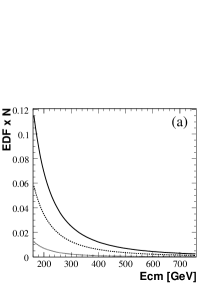
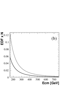
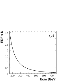
Figure 1: The unnormalized parton anti-parton Energy Density Function, $EDF\times N$ as a function of $Ecm$ for $pp$ interactions at a $\sqrt{S}=14$ TeV given by Eqs. 3 and 4. (a): The continuous, dashed and dotted lines are respectively the $EDF_{k\bar{k}}\times N_{k\bar{k}}$ dependence on $Ecm$ of the $u\bar{u}$, $d\bar{d}$ and $s\bar{s}$ systems; (b): The continuous and dashed lines are respectively the $EDF_{k\bar{k}}\times N_{k\bar{k}}$ dependence on $Ecm$ of the $d\bar{u}$ and $u\bar{d}$ systems; (c): The $gluon-gluon$ $EDF_{g\bar{g}}\times N_{g\bar{g}}$.

where the lower positive integration limits of $dx_{k}$ are set to very small, but non zero, values in order to avoid in the numerical calculations poles at $x=0$. To note is that these two last formulae are also valid for the $gluon-gluon$ $(g\bar{g})$ collisions. From the probability distribution $P(\hat{s},S)$ we derive the parton anti-parton center of mass Energy Density Functions, $EDF(k\bar{k})$, for $pp$ collisions at 14 TeV which can be parameterize above the $VV^{\prime}$ threshold as

$$EDF_{u\bar{u}}\simeq\frac{1}{N_{u\bar{u}}}\frac{3.9\times 10^{4}}{Ecm^{2.5}};\ \ \ EDF_{d\bar{d}}\simeq\frac{1}{N_{d\bar{d}}}\frac{1.956\times 10^{4}}{Ecm^{2.5}};\ \ \ EDF_{s\bar{s}}\simeq\frac{1}{N_{s\bar{s}}}\frac{1.5\times 10^{4}}{Ecm^{2.75}},$$ (3)

where $1/N_{ij}$ are the normalization factors for the colliding $k_{i}k_{j}$ partons which depend on $\sqrt{\hat{s}_{min}}$ and $\sqrt{\hat{s}_{max}}$. The $EDF$ expressions for the quark anti-quark systems $d\bar{u}$ and $u\bar{d}$, as well as the $g\bar{g}$, are respectively given by

$$EDF_{d\bar{u}}\simeq\frac{1}{N_{d\bar{u}}}\frac{1.9\times 10^{4}}{Ecm^{2}};\ \ \ EDF_{u\bar{d}}\simeq\frac{1}{N_{u\bar{d}}}\frac{4.1\times 10^{4}}{Ecm^{2}};\ \ \ EDF_{g\bar{g}}\simeq\frac{1}{N_{g\bar{g}}}\frac{55\times 10^{4}}{Ecm^{2.35}}.$$ (4)

The unnormalized $EDF$’s are shown in Fig. 1 as a function of $Ecm$. These parameterized $EDF$ expressions are applied in the following sections to the di-boson production cross sections and in particular to the $q\bar{q}\to Z^{0}Z^{0}$ reaction discussed in Sec. 4.3.

3 The $SM$ cross sections and polarizations

For the calculations of the gauge boson pair production in quark anti$-$quark and $e^{+}e^{-}$ reactions we have utilized the $SM$ helicity amplitudes tables given in Ref. [2] for the $W^{+}W^{-}$, $W^{\pm}Z^{0}$ and $Z^{0}Z^{0}$ final states. We further specify by $\tau$ the helicity states, $-1$, 0 and $+1$, of the outgoing bosons and by $\lambda$ we denote the initial fermion helicity values of $\pm 1/2$. Furthermore, the angle $\theta_{W}$ represents as usual the electro-weak mixing angle, so that the vector ($a_{Z}$) and the axial vector ($b_{Z}$) couplings of the $SM$ fermions ($f$) to the $Z^{0}$ gauge boson are given by

$$a_{Z}\ =\ \frac{1}{4sin\theta_{W}cos\theta_{W}}(r_{3}-4Qsin^{2}\theta_{W})\ ;\ \ {\rm{and}}\ \ \ b_{Z}\ =\ \frac{1}{4sin\theta_{W}cos\theta_{W}}r_{3}\ ,$$ (5)

where $Q$ is the electric charge namely, $Q\ =\ 2/3,-1/3$ and $-1$ respectively for the up, down quarks and the electron. The weak isospin projection $r_{3}$ of the fermions is equal to, $r_{3}\ =\ +1$ for the up quark while $r_{3}\ =\ -1$ is for the down quark and the electron. After integrating over the azimuthal angle, the differential cross section of the process $f\bar{f}\to VV^{\prime}$ is given in terms of the helicity amplitudes $F_{\lambda\lambda^{\prime}\tau\tau^{\prime}}$ by

$$\frac{d\sigma}{dcos\theta}\ =\ \frac{C|\vec{p}|}{16\pi\hat{s}\sqrt{\hat{s}}}\sum_{\lambda\lambda^{\prime}\tau\tau^{\prime}}|F_{\lambda\lambda^{\prime}\tau\tau^{\prime}}(cos\theta)|^{2}\ ,$$ (6)

where $\theta$ stands for the production scattering angle defined in the vector boson $VV^{\prime}$ pair rest frame between the incident fermion and the final $V$ boson momenta. The average color factor $C$ is equal to 1 for $e^{+}e^{-}$ and 1/3 for $q\bar{q}$ initial states. For a given polar angle $cos\theta$ the single and joint longitudinal polarizations $\rho_{00}(cos\theta)$ and $\rho_{0000}(cos\theta)$ are given by

$$\rho_{00}(cos\theta)\ =\ \frac{\sum_{\lambda\lambda^{\prime}\tau^{\prime}}|F_{\lambda\lambda^{\prime}0\tau^{\prime}}(cos\theta)|^{2}}{\sum_{\lambda\lambda^{\prime}\tau\tau^{\prime}}|F_{\lambda\lambda^{\prime}\tau\tau^{\prime}}(cos\theta)|^{2}}\ \ \ \ \ {\rm{and}}\ \ \ \ \ \rho_{0000}(cos\theta)\ =\ \frac{\sum_{\lambda\lambda^{\prime}}|F_{\lambda\lambda^{\prime}00}(cos\theta)|^{2}}{\sum_{\lambda\lambda^{\prime}\tau\tau^{\prime}}|F_{\lambda\lambda^{\prime}\tau\tau^{\prime}}(cos\theta)|^{2}}\ .$$ (7)

Similar expressions define the other $\rho$ elements like the $\rho_{++--}$ and $\rho_{--++}$.

In the following sections we will address our calculations to the longitudinal polarizations averaged over $cos\theta$ which we will refer to simply as $\rho_{00}$ and $\rho_{0000}$. These polarizations can be estimated from the measurement of the $cos\theta_{f}$ distributions where $\theta_{f}$ is the angle between the decay fermion direction in its parent gauge boson rest frame and the gauge boson direction in the di-boson center of mass system. Two leading methods, which are described e.g. in Ref. [4], are used to extract the polarization from the $cos\theta_{f}$ distributions. The first is by fitting it to an expression for $d\sigma/dcos\theta_{f}$ given in terms of the helicity states and the second one by applying the $\Lambda_{ij}$ helicity projection operators.

4 The reactions $f\bar{f}\to VV^{\prime}$ within the $SM$

4.1 $\bar{f}f\to W^{+}W^{-}$

The reaction $e^{+}e^{-}\to W^{+}W^{-}$ has been studied in LEP2 in the center of mass energies up to $\sim$210 GeV [5] using unpolarized electron-positron beams. The total and differential cross sections have been measured and found to be consistent with the $SM$ expectations. The $\rho_{00}$ measurements results are summarized in Table 1 where they are found to be consistent with the $SM$ expectations as estimated from our helicity amplitude calculations. The OPAL collaboration reported also on a $\rho_{0000}$ measurement [4] in the reaction $e^{+}e^{-}\to W^{+}W^{-}\to\ell\nu q\bar{q}$ at the center of mass energy of  189 GeV. Their joint polarization value of $0.201\pm 0.072(stat)\pm 0.017(syst)$ is clearly higher, but still essentially consistent within its large errors, with our calculated $SM$ expectation of 0.095 and that quoted by OPAL of 0.086$\pm$0.008.

Table 1: The LEP2 measurements of the $W$ longitudinal polarization in $e^{+}e^{-}\to W^{+}W^{-}$ reaction at an average center of mass energy of 196.6 GeV.

Experiment	$\rho_{00}$	Reference
DELPHI	0.249$\pm$0.045$\pm$0.022	[6]
L3	0.218$\pm$0.027$\pm$0.016	[7]
OPAL	0.239$\pm$0.021	[8]
$SM$ expectation	0.22	Present work

In the future ILC the electron and positron beams are planned to be longitudinal polarized. As a consequence, $\sigma(e^{+}e^{-}\to W^{+}W^{-})$ and the expected longitudinal polarizations of the final state $W^{+}$ and $W^{-}$ will depend on the polarization configuration of the initial state fermions. For an unpolarized positron and a right-handed and left-handed electron, the $e^{+}e^{-}\to W^{+}W^{-}$ cross sections as a function of the $W^{+}W^{-}$ $Ecm$ are shown in Fig. 2a.

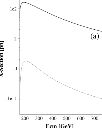
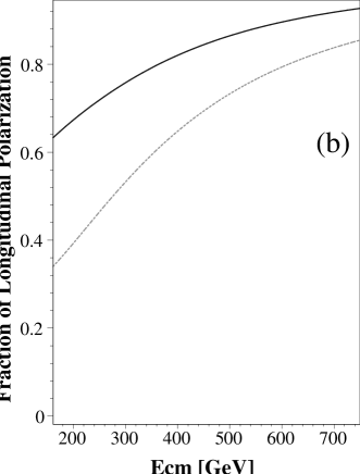
Figure 2: (a): $\sigma(e^{+}e^{-}\to W^{+}W^{-})$ as a function of the $WW$ $Ecm$. The solid line is for left-handed electrons and the dashed line is for right-handed electrons. (b): The $W$ longitudinal polarization as a function of the $WW$ $Ecm$ for a right-handed electron initial state. The solid and dashed line represent respectively the single and joint longitudinal polarization of the $W^{+}$ and $W^{-}$ bosons.

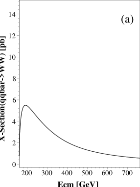
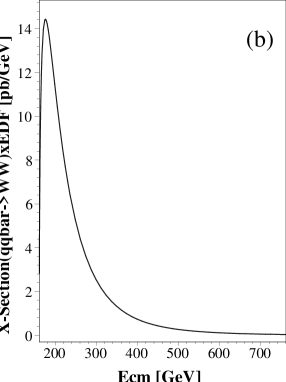
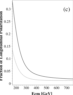
Figure 3: (a): $\sigma(\bar{q}q\to W^{+}W^{-})$ as a function of the $WW$ $Ecm$; (b): $\sigma(pp\to W^{+}W^{-})$ at $\sqrt{S_{pp}}=$14 TeV as a function of the $WW$ $Ecm$ obtained via $EDF$ from $\sigma(\bar{q}q\to W^{+}W^{-})$ and normalized to the area under the cross section shown in (a); (c): Fraction of the longitudinal polarization as a function of the $WW$ $Ecm$. The solid line is the single $W$ polarization $\rho_{00}$, and the dashed line is the joint $W^{+}W^{-}$ polarization, $\rho_{0000}$.

To note is that the cross section of the right-handed electron is much smaller than that of the left-handed electron which approaches the value of the cross section for unpolarized beams. Also of interest is the behaviour of the single and joint $W$ longitudinal polarizations (see Fig. 2b) produced by the right-handed electron, previously also dealt with in Ref. [9], which increases, rather than decreases, with energy and approach asymptotically the value of $\sim$$100\%$.

In the LHC, where the proton beams are unpolarized, the production of the final state $W^{+}W^{-}$ is dominated by unpolarized $u\bar{u}$ and $d\bar{d}$ and to a lesser extent by the $s\bar{s}$ collisions with the relative ratios of $0.63,\ 0.316\ {\rm{and}}\ 0.054$ respectively, obtained from the $PDF$ formulae. The contribution of the process $gluon\ gluon\to W^{+}W^{-}$ is estimated [10] to be of the order of $5\%$. The $\bar{q}q\to W^{+}W^{-}$ cross section as a function of $Ecm$ is shown in Fig. 3a where we sum over the $u\bar{u}$, $d\bar{d}$ and $s\bar{s}$ initial states weighted according to their occurrence in $pp$ collisions. In Fig. 3b is shown the same cross section as it will be observed in $pp$ collisions at 14 TeV by applying the relevant $EDF$. The $Ecm$ dependence of $\rho_{00}$ and $\rho_{0000}$ are illustrated in Fig. 3c where one observes that both decrease with energy and approach a nearly common flat value of $\sim$0.02. In the event that the $W^{+}W^{-}$ pair is produced in $e^{+}e^{-}$ collisions, like in LEP2, the $Ecm$ is known from the initial state, and the $W$ longitudinal polarization measurement does not present any difficulty. In the LHC however, even the single $W$ polarization measurement is not a straightforward task since the $Ecm$ value of each $W^{+}W^{-}$ event is not known from the initial $\bar{q}q$ state and in most cases also not from the final state. As is well known, for the polarization measurement one has first to identify the $W^{+}W^{-}$ event which is dealt with in length in reference [10] for their decay to the $\ell\nu\ell\nu$ and $\ell\nu\ q_{1}\bar{q}_{2}$ final states. The following requirement for the polarization measurement is the necessity to transform the $W^{+}W^{-}$ pair, including their decay products, to the $W^{+}W^{-}$ center of mass system. This requirement should a priori be more accessible in the process $W^{+}W^{-}\to q_{1}q_{2}\ q_{3}q_{4}$ than in their leptonic decay modes. However, so far an algorithm to identify in $pp$ collisions the $W^{+}W^{-}$ system via its fully hadronic decay configuration is still missing. Finally for the longitudinal polarization measurement the polar angle of the $W$ decay products has to be determined in the center of mass of the parent $W$ boson, a procedure already utilized previously [4].

4.2 The reaction $f^{\prime}{\bar{f}}\to W^{\pm}Z^{0}$

Even though the $pp\to W^{\pm}Z^{0}$ production cross section at 14 TeV is smaller by some $43\%$ than that of the $pp\to W^{+}W^{-}$, it has the advantage that the $Z^{0}$ 2-body decay modes, $\mu^{+}\mu^{-}$ and $e^{+}e^{-}$, provide a simple and clear identification and allow the measurement of its longitudinal polarization inasmuch that the $W^{\pm}Z^{0}$ center of mass system is accessible. Here we note in passing that the final states $W^{\pm}Z^{0}$ cannot be reached in $e^{+}e^{-}$ collisions.

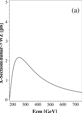
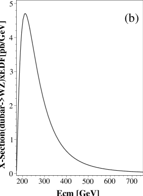
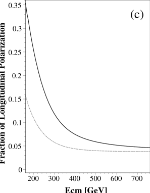
Figure 4: (a): $\sigma(d\bar{u}\to W^{-}Z^{0})$ as a function of the $WZ$ $Ecm$; (b): $\sigma(pp\to W^{-}Z^{0})$ at $\sqrt{S_{pp}}$=14 TeV as a function of the $WZ$ $Ecm$ evaluated from $\sigma(d\bar{u}\to W^{-}Z^{0})$ via the $EDF$ and normalized to the area underneath the cross section given in (a); (c): The longitudinal polarization as a function of the $WZ$ $Ecm$. The solid line is the single $Z^{0}$ polarization $\rho_{00}$ and the dashed line is the joint $W^{-}Z^{0}$ polarizations $\rho_{0000}$.

In Figs. 4a and 4b our calculated $SM$ expectations are shown for the $d\bar{u}\to W^{-}Z^{0}$ cross section as a function of $Ecm$ without and with the $EDF$ inclusion. The single $\rho_{00}(Z^{0})$ and the joint $\rho_{0000}(W^{-}Z^{0})$ longitudinal polarizations are presented in Fig. 4c as a function of $Ecm$. Like in the case of the reaction $\bar{f}f\to W^{+}W^{-}$, with the increase of energy $\rho_{00}$ and $\rho_{0000}$ are seen to approach each other to reach a low flat plateau. The experimental determination of the cross section and longitudinal polarization as a function of energy requires the possibility to calculate the $Ecm$ of the $WZ$ system. This requirement is satisfied if one is able to identify the $W^{\pm}$ boson through its decay into $q\bar{q}^{\prime}$ i.e., in a 2-jet configuration. On the other hand in the situation where the $Z^{0}$ decays to $e^{+}e^{-}$ or $\mu^{+}\mu^{-}$ and the $W^{\pm}$ decays to $e^{\pm}\nu$ or $\mu^{\pm}\nu$ one finds in general two solutions for $Ecm$ which hinders a polarization estimation.

4.3 The reaction $f{\bar{f}}\to Z^{0}Z^{0}$

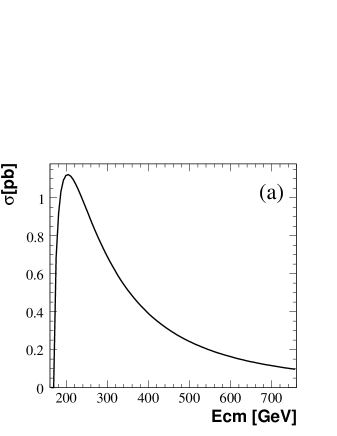
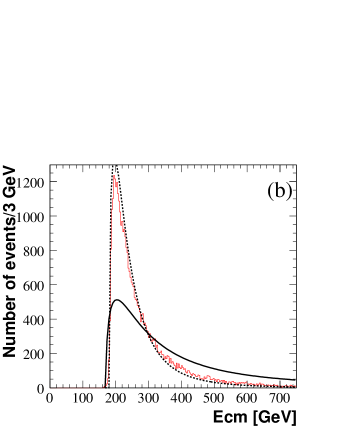
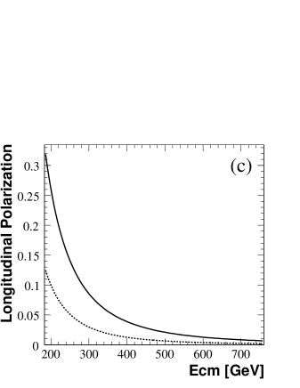
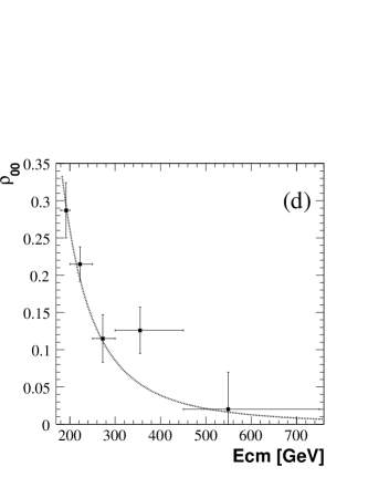
Figure 5: (a): $\sigma(q\bar{q}\to Z^{0}Z^{0})$ as a function of the $ZZ$ $Ecm$; (b): Monte Carlo (MC) generated $pp\to Z^{0}Z^{0}$ events at $\sqrt{S_{pp}}$=14 TeV as a function of the $ZZ$ $Ecm$. The solid and the dashed lines are respectively $\sigma(q\bar{q}\to Z^{0}Z^{0})$ and the corresponding $\sigma(pp\to Z^{0}Z^{0})$ at $\sqrt{S_{pp}}$=14 TeV obtained by using the $EDF$. Both lines are normalized so that the area underneath them is equal to that of the MC data histogram; (c): The calculated longitudinal polarization as a function of the $ZZ$ $Ecm$. The solid and dashed lines are respectively the single, $\rho_{00}$, and the joint, $\rho_{0000}$, longitudinal polarizations; (d): The measured $\rho_{00}$ from a MC generated $pp\to Z^{0}Z^{0}$ data sample, equivalent to $pp$ integrated luminosity of $\simeq$200 $fb^{-1}$, compared to the $SM$ expectation given by the continuous line.

The $Z^{0}Z^{0}$ system, in contrast to the $W^{\pm}Z^{0}$ and $W^{+}W^{-}$ final states, allows in most cases a straight forward determination of the center of mass energy event by event, in particular in its decay to two pairs of charged electrons or muons. Our $SM$ helicity amplitude calculation of $\sigma(q\bar{q}\to Z^{0}Z^{0})$ as a function of $Ecm$, where we sum over the $u\bar{u}$, $d\bar{d}$ and $s\bar{s}$ initial states, is shown in Fig. 5a. Since the processes $q\bar{q}\to Z^{0}Z^{0}$ is mediated, at lower order, via t-channel diagrams, it can be used to verify experimentally the $SM$ but cannot serve as a probe for the search of s-channel massive gauge bosons like the $Z^{\prime}$ or the extra dimension $Z^{\star}$ which are dealt with in the following section. As for the $gluon-gluon$ contribution to the $Z^{0}Z^{0}$ production in $pp$ collisions at 14 TeV, it is estimated to be of the order of 15$\%$[10, 11].

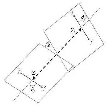
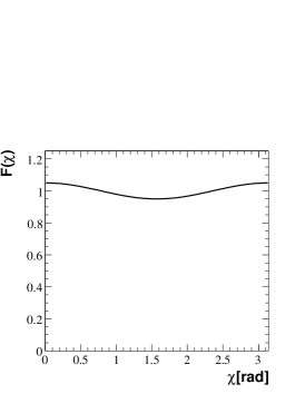
Figure 6: Left: The angle $\chi$ between the two $Z^{0}\to f\bar{f}$ decay planes in the reaction $q\bar{q}\to Z^{0}Z^{0}$ (see text); Right: The $SM$ expectation of the angular distribution $F(\chi)$ at $Ecm$=200 GeV of the $Z^{0}Z^{0}$ system, averaged over the production angle $cos\theta$.

The reliability of our derived $EDF$ expressions to transform the parton anti-parton cross sections to the corresponding $pp$ reactions is demonstrated in Fig. 5b. In this figure the data distribution of the reaction $pp\to Z^{0}Z^{0}$ at $\sqrt{S}$=14 TeV is obtained from a Pythia 6.403 generated Monte Carlo sample of $\sim$38,000 events utilizing the $PDF$ version CTEQ6L1 [12]. In the same figure $\sigma(q\bar{q}\to Z^{0}Z^{0})$ is shown by the continuous line where it is normalized to the area under the MC generated sample of the $pp$ collisions. This $q\bar{q}$ cross section is then transformed via the $EDF$ to obtain the corresponding $pp\to q\bar{q}\to Z^{0}Z^{0}$ distribution (dotted line) which again is normalized to area defined by the MC data. To be seen, there is an over all agreement between the MC sample and the expected $pp\to Z^{0}Z^{0}$ distribution. The slight deviation between the $EDF$ treated cross section and the MC generated sample distribution can be traced among other reasons to the approximate numerical evaluation of the integrals given in Eq. 2 and to the difference between the $PDF$ version incorporated in the MC program and that used by us.

The $Z^{0}Z^{0}$ single and joint longitudinal polarizations, which are shown in Fig. 5c, decrease with energy and are seen to approach each other as they reach a nearly zero value at 750 GeV. Next we calculate the single $Z^{0}$ longitudinal polarization using the generated MC sample applying the known helicity projection operator $\Lambda_{00}$ [4]. The results modified by the $EDF$ are shown in Fig. 5d for five $Ecm$ regions, each having about 900 events, where they are seen to follow the general behavior of the $SM$ expectation shown by the line drawn in the figure.

The reaction $q\bar{q}\to Z^{0}Z^{0}$, which finally decays into four charged ($e^{\pm},\mu^{\pm}$) leptons, offers another measurable variable namely, the distributions of the angle $\chi$ between the two decay planes as illustrated in Fig. 6. These planes are obtained by first transforming the whole event configuration to the $Z^{0}Z^{0}$ center of mass system and then transforming each lepton decay pair to the center of mass of its parent gauge boson. The angular distribution $F(\chi)$, which is invariant under the transformation $\chi\to\pi-\chi$, has the form [13]

$$F(\chi)\ =\ 1+Dcos(2\chi)\ ,$$ (8)

where

$$D\ =\ 0.25\times(\rho_{++--}+\rho_{--++})\ .$$ (9)

As seen from Fig. 6, in the framework of the $SM$ the $F(\chi)$ distribution at $Ecm$=200 GeV, averaged over the production angle, deviates only slightly from uniformity and thus should be very hard to detect. The study of $F(\chi)$ however may be quite useful in the case where the $Z^{0}Z^{0}$ pair is the decay product of a Higgs boson [14].

5 Detection of massive like$-$gauge vector bosons

In this section we discuss the expected effects due to the presence of a massive vector boson in the s-channel on the produced $SM$ di-gauge bosons final states. For the search of directly produced beyond the $SM$ gauge$-$like massive vector bosons, the reader is advised to consult e.g. Ref. [15] and its references therein.

5.1 The $Z^{\prime}$ boson effect on the $W^{+}W^{-}$ final state

The possible existence of heavy $Z^{\prime}$ vector bosons have been, and still are, speculated in the framework of several models [16, 17]. Searches for such heavy bosons were carried out in LEP2 and in the Tevatron which reported a lower mass limit in the region between 0.8 to 1 TeV [18]. Whereas the coupling of a $Z^{\prime}$ to fermions is expected to be similar to that of the Standard Model $Z^{0}$ ($Z^{0}_{SM}$), its coupling to $W^{+}W^{-}$ is estimated to be much weaker, namely by a factor of about 100 to 1000 [17, 18].

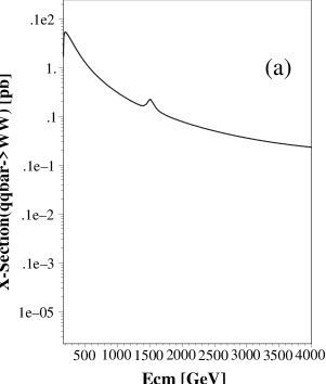
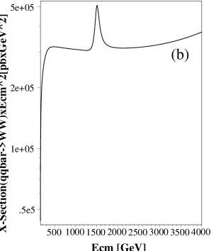
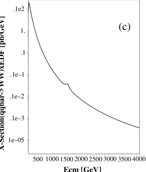
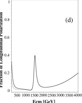
Figure 7: Features of the reaction $\bar{q}q\to W^{+}W^{-}$ in the presence of an s-channel $Z^{\prime}$, of a 1.5 TeV mass and a width of 120 GeV, as a function of the $WW$ $Ecm$. (a): $\sigma(\bar{q}q\to W^{+}W^{-})$; (b): As (a) but multiplied by $Ecm^{2}$ to check unitarity; (c): The corresponding $\sigma(pp\to W^{+}W^{-})$ at $\sqrt{S_{pp}}$=14 TeV modified by $EDF$ from $\sigma(q\bar{q}\to W^{+}W^{-})$; (d): The single (continuous line) and joint (dashed line) longitudinal polarizations as a function of the $WW$ $Ecm$.

To illustrate the feasibility to detect a $Z^{\prime}$ boson in the reaction $pp\to\gamma/Z_{SM}^{0}/Z^{\prime}\to W^{+}W^{-}$ we attributed to the $Z^{\prime}$ a mass of 1.5 TeV with a width of 120 GeV having a $SM$ like coupling to fermions while setting its coupling to the $W^{+}W^{-}$ pair weaker by a factor of 500 than that of the $Z_{SM}^{0}$ boson. In Fig. 7a $\sigma(\bar{q}q\to\gamma/Z_{SM}^{0}/Z^{\prime}\to W^{+}W^{-})$ is shown and in Fig. 7b $\sigma(\bar{q}q\to\gamma/Z_{SM}^{0}/Z^{\prime}\to W^{+}W^{-})\times Ecm^{2}$ is presented to check the unitarity requirement [19]. The corresponding distribution of $\sigma(pp\to\gamma/Z_{SM}^{0}/Z^{\prime}\to W^{+}W^{-})$ arising from $pp$ collisions at the LHC is given in Fig. 7c. From this figure it is clear that the cross section signal arising from the presence of a $Z^{\prime}(1.5)$ in the s-channel is by far too weak to be experimentally detected if only for the reason that the $pp$ luminosity at the LHC will be known to $\approx 10\%$. On the other hand, the longitudinal polarization of the $W^{+}W^{-}$ final state, shown in Fig. 7d, reveals a signal that is by approximately a factor ten larger than the $SM$ one as is estimated from Fig. 4c. Furthermore, the longitudinal polarization is seen to increase with $Ecm$ beyond the $Z^{\prime}(1.5)$ energy unlike the case where only the $Z^{0}_{SM}$ contributes in the s-channel to the $W^{+}W^{-}$ final state.

In addition to the possible existence of the $Z^{\prime}$, the conjecture of Kaluza Klein Extra Dimensions does also envisage the existence of massive excited $Z$ vector bosons, labeled as $Z^{\star}$. These couple to fermions as the $Z_{SM}^{0}$ [20] and the mass of the lightest one of them is currently estimated to be equal or larger than $\sim$4 TeV. Inasmuch that these massive vector bosons do have a sufficiently strong coupling to the $W^{+}W^{-}$ boson pair, they may be detected as a resonance in the $W^{+}W^{-}$ invariant mass distributions. If their coupling strength to $W^{+}W^{-}$ is similar to that chosen by us for the $Z^{\prime}$, then their longitudinal polarization behaviour follows the one shown in Fig. 7d and could be instrumental in the detection of these massive vector bosons.

5.2 The $W^{\prime}$ boson effect on the $W^{\pm}Z^{0}$ final states

The existence of massive $W^{\prime}$ or a $W^{\prime}-$like bosons are now a common prediction of several beyond the $SM$ physics scenarios where their properties, and in particular their couplings to fermions and their trilinear coupling $W^{\prime}WZ$, are dealt with in various investigations [15].

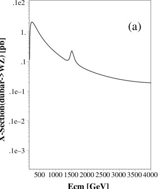
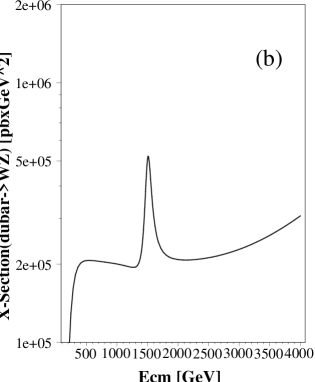
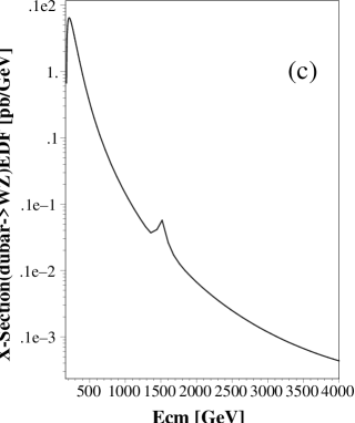
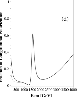
Figure 8: Features of the reaction $d\bar{u}\to W^{-}Z^{0}$ in the presence of a 1.5 TeV $W^{\prime}$ with a width of 120 GeV as a function of the $WZ$ $Ecm$. (a): $\sigma(d\bar{u}\to W^{-}Z^{0})$; (b): $\sigma(d\bar{u}\to W^{-}Z^{0})\times Ecm^{2}$ for unitarity check; (c): $\sigma(pp\to W^{-}Z^{0})$ at $\sqrt{S_{pp}}$=14 TeV modified via $EDF$ from $\sigma(d\bar{u}\to W^{-}Z^{0})$; (d): The longitudinal polarization. The solid line is $\rho_{00}$ the single $Z$ polarization, and the dashed line is $\rho_{0000}$, the joint $W^{-}Z^{0}$ polarization.

Here we examine the effect of the presence of a 1.5 TeV $W^{\prime}$ vector boson in the s-channel having a 120 GeV width which has a $SM$ like couplings to fermions but a $W^{\prime}WZ$ coupling smaller by a factor 500 than the corresponding $WWZ$ one. The resulting cross section for the reaction $d\bar{u}\to W/W^{\prime}\to W^{-}Z^{0}$ is shown in Fig. 8a. This cross section, multiplied by $Ecm^{2}$ is shown in Fig. 8b to verify the unitarity condition. The signal of $W^{\prime}$ presence in the $W^{-}Z^{0}$ production in the $pp$ reactions, seen in Fig. 8c, is far too weak to be noticed. On the other hand, the longitudinal polarization signal at 1.5 TeV and its behaviour at energies above it (see Fig. 8d) is considerably higher than that expected in the absence of a $W^{\prime}$ gauge boson in the s-channel.

6 Summary

In the frame work of the Standard Model the reactions $q\bar{q}\to VV^{\prime}$ are calculated via the helicity amplitudes for the final states $W^{+}W^{-}$, $W^{\pm}Z^{0}$ and $Z^{0}Z^{0}$ to obtain their cross sections and longitudinal polarizations as a function of their center of mass energy, $Ecm$. These cross sections are transformed to the corresponding ones expected to be observed in $pp$ collisions at 14 TeV, by using our parameterizations for the $q\bar{q}$ Energy Density Functions. These expressions for the $EDF$ may also be useful for the opposite transformation, that is, from the $pp$ processes to the basic parton anti-parton cross sections.

Whereas in the LHC the cross section measurement accuracy depends above all on the luminosity precision, currently estimated to be $10\%$, clearly one of the polarization measurement virtues is its independence of the luminosity. The single and joint longitudinal polarization of the $VV^{\prime}$ final states in $pp$ collisions are seen to decrease and approach each other as $Ecm$ increases. Whereas at present the polarization measurements of the $W^{+}W^{-}$ final state are not feasible, they are accessible in the $Z^{0}Z^{0}$ channel. Methods to measure to a good approximation the longitudinal polarizations of the $W^{\pm}Z^{0}$ final state is likely to be worked out in the future.

The effect on the production of the $VV^{\prime}$ states from the existence of s-channel massive bosons like the $Z^{\prime}$, $W^{\prime}$ and the $ED$ heavy $Z^{\star}$, is studied with the results that the change in the polarization structures are more pronounced than those seen in the behaviour of the cross sections.

Acknowledgements
Our thanks are due to members of the Tel-Aviv University ATLAS group, and in particular to E. Etzion, for their continuous support throughout this work. In addition we are grateful to Y. Oz and S. Nussinov for their helpful discussions and suggestions.

References

- [1] “International Linear Collider reference design report”, ILC-REPORT-2007-001.
- [2] E. Nuss, Z. Phys. C76 (1997) 701 and references therein.
- [3] W.K. Tung et al., JHEP 0702:053,2007, hep-ph/0611254.
- [4] OPAL Coll., G. Abbiendi et al., Eur. Phys. J. C19 (2001) 229.
- [5] See e.g., S. Mele in “Physics of bosons at LEP”, CERN-PH-EP/2004-030, July 6, 2004, To appear in a special issue of Physics Report celebrating the 50th anniversary of CERN.
- [6] DELPHI Coll., J. Abdallah et al., Eur. Phys. J. C54 (2008) 345.
- [7] L3 Coll., P. Achard et al., Phys. Lett. B557 (2003) 147.
- [8] OPAL Coll., G. Abbiendi et al., Phys. Lett. B585 (2004) 223.
- [9] P. Poulose, Phys. Lett. B534 (2002) 131.
- [10] T. Barber et al., ATLAS CSC NOTE, “DiBoson Physics Studies with the ATLAS Detector”, ATL-PHYS-PUB-2007-xxxx.
- [11] T. Binoth et al., “Gluon-induced QCD corrections to ”, atXiv:0807.0024v1
- [12] J. Pumplin et al., JHEP 0207:012,2002 hep-ph/0201195.
- [13] M.J. Duncan, G.L. Kane, W.W. Repko, Nucl. Phys. B272 (1986) 517.
- [14] C.P. Buszello et al., Eur.Phys. J. C32 (2004) 209.
- [15] See e.g. T.G. Rizzo, JHEP 0705:037,2007 and references therein.
- [16] See e.g., G. Altarelli, B. Mele, M. Ruiz-Altaba, Z. Phys. C45 (1989) 109; M. Schäfer et al., “ studies in full simulation (DCI)”, ATL-PHYS-PUB-2005-010; F. Ledroit et al., “ at LHC”, ATL-PHYS-PUB-2006-024.
- [17] See e.g., M. Carena, A. Daleo, B.A. Dobrescu, T.M.P. Tait, Phys. Rev. DC70 (2004) 093009.
- [18] P. Langacker, “The Physics of Heavy Z’ Gauge Bosons”, arXiv:0801.1345v2.
- [19] See e.g. J.M. Cornwall, D.N. Levin, G. Tiktopoulos, Phys. Rev. D10 (1974) 1145.
- [20] See e.g., I. Antoniadis, Phys. Lett. B246 (1990) 377; I. Antoniadis, C. Munoz and M. Quiros, Nucl. Phys. B397 (1993) 515; I. Antoniadis and K. Benakli, superstrings,” Phys. Lett. B326 (11994) 69; I. Antoniadis and K. Benakli, Int. J. Mod. Phys. A15, (2000) 4237; I. Antoniadis and K. Benakli, M. Quiros, Phys. Lett. B331 (1994) 313.