Reduced fidelity susceptibility and its finite-size scaling behaviors in the Lipkin-Meshkov-Glick Model

Abstract

We derive a general formula of the reduced fidelity susceptibility when the reduced density matrix is $2\times 2$ block-diagonal. By using this result and the continuous unitary transformations, we study finite-size scaling of the reduced fidelity susceptibility in the Lipkin-Meshkov-Glick Model. It is found that it can be used to characterize quantum phase transitions, implying that we can extract information of quantum phase transitions only from the fidelity of a subsystem, which is of practical meaning in experiments.

I Introduction

During the past few years, some important concepts in quantum information theory have been introduced to characterize quantum phase transitions (QPTs). For example, entanglement, which is one of the central concepts in quantum information theory, has been investigated extensively in QPTs in various models, like Ising model Osterloh et al. (2002); Vidal et al. (2004a); Latorre et al. (2005); Barthel et al. (2006) and Lipkin-Meshkov-Glick (LMG) model Vidal et al. (2004b). Recently, fidelity, which is another important quantum information concept, has also been applied in characterizing QPTs. The introducing of fidelity in QPTs is natural Quan et al. (2006); Zanardi and Paunković (2006); Buonsante and Vezzani (2007); Zanardi et al. (2007); Cozzini et al. (2007); You et al. (2007); Zhou and Barjaktarevic (2007); Zhou et al. (2007); Zhou (2007); Venuti and Zanardi (2007); Gu et al. (2007); Chen et al. (2007); Ning et al. (2008); Kwok et al. (2008); Yang (2007); Zhao and Zhou (2008); Chen et al. (2008); Yang et al. (2008), since it’s mathematically the overlap between two states, while QPTs are just dramatic changes in ground-state properties. However, the fidelity used in the study of QPTs depends computationally on an arbitrary yet finite small change of the driving parameter. To cancel the arbitrariness, Zanardi et al. introduced the Riemannian metric tensor Venuti and Zanardi (2007), while You et al. suggested the fidelity susceptibility You et al. (2007). The fidelity susceptibility then becomes an effective tool to study critical properties Venuti and Zanardi (2007); Gu et al. (2007) in many-body systems.

It’s noticed that all the above works are concentrated on the fidelity of the global ground states, and we may call this kind of fidelity susceptibility the global fidelity susceptibility. However, in experiments, one always probe the subsystem but not the whole system for practical convenience. Here we use the reduced fidelity Gorin et al. (2006) (also called partial fidelity in Paunkovic et al. (2008); guparfide (2008)) susceptibility (RFS), which describes the fidelity susceptibility of a subsystem. In this work, first we derive a general formula of the reduced fidelity susceptibility when the reduced density matrix is $2\times 2$ block-diagonal. Then, considering the LMG model, we show that the RFS can be used to characterize QPTs, and find that the scaling exponent is different from that of the global fidelity susceptibility.

This paper is organized as follows. In Sec. II, we briefly review the concept of fidelity susceptibility, and give a general formula of RFS for a special but interesting case that the density matrix is $2\times 2$ block-diagonal. Then in Sec. III, we introduce the LMG model Lipkin et al. (1965). in the isotropic case, we find that the critical behavior of RFS $\chi$ in response to magnetic transverse field $h$ as $(h_{c}-h)^{-1}$ in thermodynamic limit. While in the anisotropic case, by using the continuous unitary transformations (CUTs) Wegner (1994); Glazek and Wilson (1993, 1994), we find that the maximum of $\chi$ over $h$ diverged as $N^{2/3}$ for an $N$-spin system, and $\left|h_{c}-h\right|^{-1}$ in thermodynamic limit. Finally, we perform a numerical scaling analysis, and the results are well consistent with our theoretical ones.

II Reduced Fidelity Susceptibility

We first give a brief review on the concept of fidelity susceptibility. The Hamiltonian of a quantum system undergoing QPTs can be written as

$$H\left(h\right)=H_{0}+hH_{I},$$ (1)

where $H_{I}$ is supposed to be the driving term with control parameter $h$. The global fidelity is defined as $F\left(h,\delta\right)=\left|\langle\varphi_{0}\left(h\right)|\varphi_{0}\left(h+\delta\right)\rangle\right|$, where $|\varphi_{0}\left(h\right)\rangle$ is the ground state of $H\left(h\right)$, and $\delta$ is a small quantity. The reduced fidelity is defined as the overlap between the reduced density matrix (RDM) $\rho\left(h\right)$ of the ground state $|\varphi_{0}\left(h\right)\rangle$. In the follows, we take $\rho\equiv\rho\left(h\right)$ and $\tilde{\rho}\equiv\rho\left(h+\delta\right)$. Then the reduced fidelity is given by Uhlmann (1976)

$$F\left(h,\delta\right)=\text{tr}\sqrt{\rho^{1/2}\tilde{\rho}\rho^{1/2}}.$$ (2)

The corresponding fidelity susceptibility is defined as Zanardi and Paunković (2006); You et al. (2007)

$$\chi=\lim_{\delta\rightarrow 0}\frac{-2\ln F}{\delta^{2}},$$ (3)

and then we could write $F\simeq 1-\chi\delta^{2}/2$.

In this papar we consider that the RDM is block-diagonal,

$$\rho=\bigoplus\limits_{i=1}^{n}\varrho_{i},$$ (4)

where $\varrho_{i}$’s are $2\times 2$ semi-positive definite Hermitian matrices, since $\rho$ is a density matrix. Now we introduce some useful formulas at first. Let $A$ and $B$ are arbitrary $2\times 2$ semi-positive definite matrices, then we have

$$\text{tr}\sqrt{A^{1/2}BA^{1/2}}=\sqrt{\text{tr}\left(AB\right)+2\sqrt{\det\left(AB\right)}},$$ (5)

and if $A=B$, it becomes

$$\text{tr}\left(A^{2}\right)=\left(\text{tr}A\right)^{2}-2\det A.$$ (6)

Take derivations of the above equation with respect to some variable $h$, we get

$$\text{tr}\left(AA^{\prime}\right) =\text{tr}A\text{tr}A^{\prime}-\partial_{h}\left(\det A\right),$$ (7)

$$\text{tr}\left(AA^{\prime\prime}\right) =\text{tr}A\text{tr}A^{\prime\prime}-\partial_{h}^{2}\left(\det A\right)+2\det A^{\prime},$$ (8)

where $A^{\prime}\equiv\partial_{h}A$, $A^{\prime\prime}\equiv\partial_{h}^{2}A$ and $\partial_{h}$tr$\left(A\right)=$tr$\left(A^{\prime}\right)$. Now the fidelity can be written as

$$F =\sum_{i=1}^{n}\text{tr}\sqrt{\varrho_{i}^{1/2}\tilde{\varrho}_{i}\varrho_{i}^{1/2}}$$

$$=\sum_{i=1}^{n}\sqrt{\text{tr}\varrho_{i}\tilde{\varrho}_{i}+2\sqrt{\det\varrho_{i}\tilde{\varrho}_{i}}},$$ (9)

and recall that $F\simeq 1-\chi\delta^{2}/2$, the susceptibility $\chi=\sum_{i=1}^{n}\chi_{i}$, with $\chi_{i}$ corresponds to the ‘susceptibility’ of the $i$-th block in Eq. (4). To obtain the susceptibility, we should expand the fidelity with respect to $\delta$, and for $\tilde{\varrho}_{i}$ $\simeq$ $\varrho_{i}\left(h\right)+\varrho_{i}^{\prime}\left(h\right)\delta+\delta^{2}\varrho_{i}^{\prime\prime}\left(h\right)/2+O\left(h^{3}\right)$, we have

$$\left\{\begin{aligned} &\text{tr}\left(\varrho\tilde{\varrho}\right)\simeq\text{tr}\left(\varrho^{2}\right)+\text{tr}\left(\varrho\varrho^{\prime}\right)\delta+\frac{\delta^{2}}{2}\text{tr}\left(\varrho\varrho^{\prime\prime}\right),\\ &\det\tilde{\varrho}\simeq\det\varrho+\partial_{h}\left(\det\varrho\right)\delta+\frac{\delta^{2}}{2}\partial_{h}^{2}\left(\det\varrho\right),\end{aligned}\right.$$ (10)

here we omit the subscript $i$ for convenience.

In the case that $\det\varrho\neq 0$, we have tr$\varrho\neq 0$ since $\varrho$ is semi-positive definite. Then we get

$$\sqrt{\det\left(\varrho\tilde{\varrho}\right)} \simeq\det\varrho+\frac{\delta}{2}\partial_{h}\det\varrho$$

$$+\frac{\delta^{2}}{4}\left[\partial_{h}^{2}\det\varrho-\frac{\left(\partial_{h}\det\varrho\right)^{2}}{2\det\varrho}\right].$$ (11)

Take the above expression into Eq. (9) and with the help of Eqs. (6), (7) and (8) we obtain

$$\text{tr}\sqrt{\varrho^{1/2}\tilde{\varrho}\varrho^{1/2}}\simeq\text{tr}\varrho+\frac{\delta}{2}\text{tr}\varrho^{\prime}+\frac{\delta^{2}}{4}\text{tr}\varrho^{\prime\prime}$$

$$+\frac{\delta^{2}}{8\text{tr}\varrho}\left\{4\det\varrho^{\prime}-\left(\text{tr}\varrho^{\prime}\right)^{2}-\frac{\left[\partial_{h}\det\left(\varrho\right)\right]^{2}}{\det\left(\varrho\right)}\right\}.$$ (12)

If $\det\varrho=0$ but tr$\varrho\neq 0$,  we have $\det\left(\varrho\tilde{\varrho}\right)=0$. Moreover, since $\varrho$ is positive semi-definite, zero is the lower bound of $\det\varrho$, which requires $\partial_{h}\det\varrho=0$ and $\partial_{h}^{2}\det\varrho>0$. Thus we have

$$\text{tr}\left(\varrho\tilde{\varrho}\right) =\left(\text{tr}\varrho\right)^{2}+\text{tr}\varrho\text{tr}\varrho^{\prime}\delta$$

$$+\frac{\delta^{2}}{2}\left[\text{tr}\varrho\text{tr}\varrho^{\prime\prime}-\partial_{h}^{2}\left(\det\varrho\right)+2\det\varrho^{\prime}\right],$$ (13)

and

$$\text{tr}\sqrt{\varrho^{1/2}\tilde{\varrho}\varrho^{1/2}} \simeq\text{tr}\varrho+\frac{\delta}{2}\text{tr}\varrho^{\prime}+\frac{\delta^{2}}{4}\text{tr}\varrho^{\prime\prime}$$

$$+\frac{\delta^{2}}{8\text{tr}\varrho}\left[4\det\varrho^{\prime}-\left(\text{tr}\varrho^{\prime}\right)^{2}-2\partial_{h}^{2}\left(\det\varrho\right)\right].$$ (14)

In the last case that tr$\varrho=0$, $\varrho$ is equivalent to a zero matrix, since $\varrho$ is Hermitian. Then tr$\left(\varrho\tilde{\varrho}\right)=\sqrt{\det\left(\varrho\tilde{\varrho}\right)}=0$, and $F=0$.

Conclude the above three cases, we get the ‘susceptibility’ for block $\varrho_{i}$ as

$$\chi_{i}=\left\{\begin{split}&\frac{1}{4\text{tr}\varrho_{i}}\left\{\left(\text{tr}\varrho_{i}^{\prime}\right)^{2}-4\det\varrho_{i}^{\prime}+\frac{\left[\partial_{h}\det\left(\varrho_{i}\right)\right]^{2}}{\det\left(\varrho_{i}\right)}\right\}\quad&\text{for}\quad&\text{tr}\varrho_{i}\neq 0,\det\varrho_{i}\neq 0,\\ &\frac{1}{4\text{tr}\varrho_{i}}\left[\left(\text{tr}\varrho_{i}^{\prime}\right)^{2}-4\det\varrho_{i}^{\prime}+2\partial_{h}^{2}\left(\det\varrho_{i}\right)\right]\quad&\text{for}\quad&\text{tr}\varrho_{i}\neq 0,\det\varrho_{i}=0,\\ &0\quad&\text{for}\quad&\text{tr}\varrho_{i}=0,\end{split}\right.$$ (15)

where the terms of $\delta\text{tr}\varrho^{\prime}/2$ and $\delta^{2}\text{tr}\varrho^{\prime\prime}/4$ in Eqs. (12) and (14) are canceled in the final expression of the fidelity, due to tr$\left(\rho\right)\equiv 1$, and tr$\left(\rho^{\prime}\right)=\text{tr}\left(\rho^{\prime\prime}\right)=0$.

Finally, we consider a more special case that $\rho$ is diagonal, the then susceptibility is obtained readily

$$\chi=\sum_{i=1}^{n}\frac{\left(\lambda_{i}^{\prime}\right)^{2}}{4\lambda_{i}},$$ (16)

where $\lambda_{i}$’s are the nonzero diagonal terms.

III The LMG Model and its scaling exponents of RFS

III.1 The LMG model and RFS

The LMG model was introduced in nuclear physics to describe mutually interacting spin-1/2 particles, embedded in a transverse magnetic field. In the thermodynamic limit, it undergoes a QPT that is described by the mean field analysis Botet et al. (1982). Recently the finite-size scaling was studied by the $1/N$ expansion in the Holstein-Primakoff single boson representation Botet and Jullien (1983) and by the CUTs Dusuel and Vidal (2004, 2005). The Hamiltonian of the LMG model reads

$$H= H_{0}+hH_{I}$$

$$= -\frac{\lambda}{N}\left(1+\gamma\right)\left(\mathbf{S}^{2}-S_{z}^{2}-N/2\right)$$

$$-\frac{\lambda}{2N}\left(1-\gamma\right)\left(S_{+}^{2}+S_{-}^{2}\right)-2hS_{z},$$ (17)

where $S_{\alpha}=\sum_{i}\sigma_{i\alpha}/2$, with $\sigma_{\alpha}\left(\alpha=x,y,z\right)$ the Pauli matrices, and $S_{\pm}=S_{x}\pm iS_{y}$. The prefactor $1/N$ ensures finite energy per spin in the thermodynamic limit. In the context, we set the parameters: $\lambda=1$, $\left|\gamma\right|\leq 1$, $h\geq 0$. We take $h\geq 0$ as the spectrum is invariant under the transformation $h\leftrightarrow-h$. In addition, we only consider the maximum spin sector $S=N/2$ in which the lowest energy state lies.

Now we consider a 2-body RDM of the LMG model Wang and Mølmer (2002)

$$\rho_{ij}=\begin{pmatrix}v_{+}&0&0&u\\ 0&y&y&0\\ 0&y&y&0\\ u&0&0&v_{-}\end{pmatrix},$$ (18)

in the standard basis $\left\{|00\rangle,|01\rangle,|10\rangle,|11\rangle\right\}$, where $\sigma_{z}|0\rangle=-|0\rangle$ and $\sigma_{z}|1\rangle=|1\rangle$, while the nonzero matrix elements reads

$$v_{\pm} =\frac{N^{2}-2N+4\left\langle S_{z}^{2}\right\rangle\pm 4\left\langle S_{z}\right\rangle\left(N-1\right)}{4N\left(N-1\right)},$$

$$y =\frac{N^{2}-4\left\langle S_{z}^{2}\right\rangle}{4N\left(N-1\right)},\quad u=\frac{\left\langle S_{x}^{2}-S_{y}^{2}\right\rangle}{N\left(N-1\right)},$$ (19)

where $\left[A,B\right]_{+}=AB+BA$ is the anti-commutator for operators $A$ and $B$. The zero elements of $\rho_{ij}$ result from the fact that the total spin and the parity are conserved quantities, i.e.,

$$\left[H,S^{2}\right]=\left[H,\prod_{i=1}^{N}\sigma_{iz}\right]=0.$$ (20)

It’s noticed that $\rho_{ij}$ is actually block-diagonal in the rearranged basis $\{|00\rangle,|11\rangle,|01\rangle,|10\rangle\}$, and the two blocks are

$$\varrho_{1}=\begin{pmatrix}v_{+}&u\\ u&v_{-}\end{pmatrix},\varrho_{2}=\begin{pmatrix}y&y\\ y&y\end{pmatrix}.$$ (21)

With the help of Eq. (15), we can give the RFS explicitly

$$\chi = \frac{y^{\prime 2}}{2y}+\frac{1}{4\left(v_{+}+v_{-}\right)}{\biggl{[}}\left(v_{+}^{\prime}-v_{-}^{\prime}\right)^{2}+4u^{\prime 2}$$ (22)

$$+\frac{\left(v_{+}^{\prime}v_{-}+v_{+}v_{-}^{\prime}-2u^{\prime}u\right)^{2}}{\left(v_{+}v_{-}-u^{2}\right)}{\biggl{]},}$$

here we consider the case that $\det\varrho_{1}\neq 0$, and the following computations are based on the above formula.

III.2 The isotropic case

Firstly, we consider the isotropic case, $\gamma=1$, and the Hamiltonian reads

$$H=-\frac{2}{N}\left(\mathbf{S}^{2}-S_{z}^{2}-N/2\right)-2hS_{z},$$ (23)

which is diagonal in the standard eigenbasis $\left\{|S,M\rangle\right\}$ of $\mathbf{S}^{2}$ and $S_{z}$. For $S=N/2$ the eigenstates are

$$E\left(M,h\right)=\frac{2}{N}\left(M-\frac{hN}{2}\right)^{2}-\frac{N}{2}\left(1+h^{2}\right),$$ (24)

and the ground state is readily obtained when

$$M_{0}=\left\{\begin{aligned} &N/2&\text{for}\quad&h\geq 1,\\ &N/2-R\left[N(1-h)/2\right]&\text{for}\quad&0\leq h<1,\end{aligned}\right.$$ (25)

where $R(x)\equiv\text{round}(x)$. Then one can see level crossings exist at $h=h_{j}$, where $h_{j}=1-\left(2j+1\right)/N$, between the two states $|N/2,N/2-j\rangle$ and $|N/2,N/2-j-1\rangle$. In the thermodynamic limit, these critical points form a region of criticality.

The elements of the RDM in ground state are readily obtained as

$$v_{\pm} =\frac{\left(N\pm 2M_{0}\right)\left(N-2\pm 2M_{0}\right)}{4N\left(N-1\right)},$$

$$y =\frac{\left(N^{2}-4M_{0}\right)}{4N\left(N-1\right)},\quad u=0.$$ (26)

As $N$ is very large, $M_{0}\left(h<1\right)\simeq hN/2$. With Eq. (22), we obtain the susceptibility in thermodynamic limit

$$\lim_{N\rightarrow\infty}\chi\left(h>1-\frac{1}{N}\right)\simeq\frac{1}{2\left(1-h^{2}\right)}.$$ (27)

Obviously, the asymptotic behavior of $\chi$ as $h\rightarrow 1$ is $1/\left(1-h\right)$. However, there is no QPT in its symmetric phase $h>1$, because the ground state is independent of $h$.

III.3 The anisotropic case

III.3.1 Spin expectation values

Next we consider the anisotropic case, and the numerical results of the RFS as a function of $h$ are shown in Fig. (43). We adopt the $1/N$ expansion method with CUTs that was used extensively by Dusuel and Vidal Dusuel and Vidal (2004, 2005), which corresponds to the large $N$ limit. While the Holestein-Primakoff method is not suitable for our task since it could only give a first order correction in a $1/N$ expansion.

Here we firstly recall the CUTs introduced by Wegner Wegner (1994) and independently by Glazek and Wilson Glazek and Wilson (1993, 1994). For a pedagogical introduction to this technique, one can see Dusuel and Uhrig (2004). The main idea of CUTs is to diagonalize the Hamiltonian in a continuous way starting from the original Hamiltonian $H=H\left(l=0\right)$. A flowing Hamiltonian is then defined by

$$H\left(l\right)=U^{\dagger}\left(l\right)H\left(0\right)U\left(l\right),$$ (28)

where $U\left(l\right)$ is unitary and $l$ is a scaling parameter such that $H\left(l=\infty\right)$ is diagonal. A derivation of the Eq. (28) with respect to $l$ yields the flow equation

$$\partial_{l}H\left(l\right)=\left[\eta\left(l\right),H\left(l\right)\right],$$ (29)

where $\eta\left(l\right)=-U^{\dagger}\partial_{l}U$ is an anti-Hermitian generator. To obtain the expectation value of any operator $\Omega$ on an eigenstate $|\psi\rangle$ of $H$, one should follow the flow of the operator $\Omega\left(l\right)=$ $U^{\dagger}\left(l\right)H\left(0\right)U\left(l\right)$, by solving Eq. (29). Fortunately the results of the spin expectation values have been obtained by Dusuel and Vidal in Dusuel and Vidal (2004, 2005), and here we’ll compute the scaling behavior of the derivatives of these values.

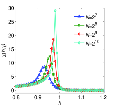
Figure 1: Fidelity susceptibility $\chi$ as a function of $h$ with various system size $N=2^{7},2^{8},2^{9},2^{10}$. The positions of their peaks approach to the critical point $h_{c}=1$ .

Firstly, we consider the system size $N$ is very large, and the matrix elements are rewritten as

$$v_{\pm} = \frac{1}{4}+\frac{\left\langle S_{z}^{2}\right\rangle}{N^{2}}\pm\frac{\langle S_{z}\rangle}{N},$$

$$y = \frac{1}{4}-\frac{\left\langle S_{z}^{2}\right\rangle}{N^{2}},\quad u=\frac{\left\langle S_{x}^{2}\rangle-\langle S_{y}^{2}\right\rangle}{N^{2}}.$$ (30)

The spin expectation values appeared in the above expressions can be solved by the CUTs with $1/N$ expansion. For symmetry phase ($h>1$), we have

$$\frac{2\langle S_{z}\rangle}{N}= 1+\frac{1}{N}\left(\frac{P_{z}^{\left(1\right)}}{G^{1/2}}+1\right)+\frac{\left(1-\gamma\right)^{2}}{N^{2}}\left(\frac{P_{z}^{\left(2\right)}}{G^{2}}+\frac{Q_{z}^{\left(2\right)}}{G^{3/2}}\right)+\frac{\left(1-\gamma\right)^{2}}{N^{3}}\left(\frac{P_{z}^{\left(3\right)}}{G^{7/2}}+\frac{Q_{z}^{\left(3\right)}}{G^{3}}\right)+O\left(\frac{1}{N^{4}}\right),$$

$$\frac{4\langle S_{x}^{2}\rangle}{N^{2}}= \left(h-\gamma\right)\left\{\frac{1}{NG^{1/2}}+\frac{1}{N^{2}}\left(\frac{P_{xx}^{\left(2\right)}}{G^{2}}+\frac{Q_{xx}^{\left(2\right)}}{G^{3/2}}\right)+\frac{1}{N^{3}}\left(\frac{P_{xx}^{\left(3\right)}}{G^{7/2}}+\frac{Q_{xx}^{\left(3\right)}}{G^{3}}\right)\right\}+O\left(\frac{1}{N^{4}}\right),$$

$$\frac{4\langle S_{y}^{2}\rangle}{N^{2}}= \frac{1}{h-\gamma}\left\{\frac{G^{1/2}}{N}+\frac{1}{N^{2}}\left(\frac{P_{yy}^{\left(2\right)}}{G}+\frac{Q_{yy}^{\left(2\right)}}{G^{1/2}}\right)+\frac{1}{N^{3}}\left(\frac{P_{yy}^{\left(3\right)}}{G^{5/2}}+\frac{Q_{yy}^{\left(3\right)}}{G^{2}}\right)\right\}+O\left(\frac{1}{N^{4}}\right),$$

$$\frac{4\langle S_{z}^{2}\rangle}{N^{2}}= 1+\frac{1}{N}\left(\frac{P_{zz}^{\left(1\right)}}{G^{1/2}}+2\right)+\frac{1}{N^{2}}\left(\frac{P_{zz}^{\left(2\right)}}{G^{2}}+\frac{Q_{zz}^{\left(2\right)}}{G^{3/2}}\right)+\frac{\left(1-\gamma\right)^{2}}{N^{3}}\left(\frac{P_{zz}^{\left(3\right)}}{G^{7/2}}+\frac{Q_{zz}^{\left(3\right)}}{G^{3}}\right)+O\left(\frac{1}{N^{4}}\right),$$ (31)

where $G\equiv G\left(h,\gamma\right)=\left(h-1\right)\left(h-\gamma\right)$. Here we do not present $P_{\xi}^{\left(i\right)}\equiv P_{\xi}^{\left(i\right)}\left(h,\gamma\right)$ and $Q_{\xi}^{\left(i\right)}\equiv Q_{\xi}^{\left(i\right)}\left(h,\gamma\right)$ ($i=1,2,3$ and $\xi=z,xx,yy,zz$), which are polynomials of $h$ and $\gamma$, whereas of little meaning for computing the scaling exponents. For more details, you can refer to the appendix part of Dusuel and Vidal (2005). It’s noticed that, the above expressions can be written in the form

$$\Phi_{N}\left(h,\gamma\right)=\Phi_{N}^{\text{reg}}\left(h,\gamma\right)+\Phi_{N}^{\text{sing}}\left(h,\gamma\right),$$ (32)

where the superscripts ‘reg’ and ‘sing’ stand for regular and singular respectively. A nonsingular contribution is understood to be a function of $h$ which is nonsingular at $h=1$, as well as all its derivatives. Take $2\langle S_{z}\rangle/N$ for example, the regular part is $1+1/N$ and the remaining forms the singular part. As $h$ approaches to $1$, the terms involving $Q_{\xi}^{\left(i\right)}$’s are small compared to the terms involving $P_{\xi}^{\left(i\right)}$’s by a factor $G\left(h,\gamma\right)$, hence we could only consider the terms involving $P_{\xi}^{\left(i\right)}$’s.

III.3.2 Finite-size scaling

Here we show how to derive the finite-size scaling exponents of the spin expectation values and their derivatives, and take $2\langle S_{z}\rangle/N$ for example,

$$\frac{2\langle S_{z}\rangle}{N} = 1+\frac{1}{N}+\frac{1}{NG^{1/2}}{\biggl{\{}}P_{z}^{\left(1\right)}+\frac{\left(1-\gamma\right)^{2}P_{z}^{\left(2\right)}}{NG^{3/2}}$$ (33)

$$+\frac{\left(1-\gamma\right)^{2}P_{z}^{\left(3\right)}}{\left(NG^{3/2}\right)^{2}}+O\bigg{(}\frac{1}{\left[NG^{3/2}\right]^{3}}\bigg{)}{\biggl{\}},}$$

where the singular part (terms after $1+1/N$) can be written in the form

$$\left(\frac{2\langle S_{z}\rangle}{N}\right)^{\text{sing}}\simeq\frac{1}{NG\left(h,\gamma\right)^{1/2}}\mathscr{F}_{S_{z}}\left[NG\left(h,\gamma\right)^{3/2},\gamma\right],$$ (34)

where $\mathscr{F}_{\Phi}$ ($\Phi=S_{z},S_{x}^{2},S_{y}^{2},S_{z}^{2}$) is a scaling function for these spin expectation values. While in fact that there can be no singularity in any physical quantity in a finite-size system, and the critical point $h_{c}=1$ only for thermodynamic limit $N\rightarrow\infty$. This implies that the singularity of $G\left(h,\gamma\right)^{-1/2}$ has to be canceled by the one of $\mathscr{F}_{S_{z}}\left[NG\left(h,\gamma\right)^{3/2},\gamma\right]$. Thus one must have $\mathscr{F}_{S_{z}}\left(x,\gamma\right)\sim x^{-1/3}$, which in turn implies the following finite size scaling:

$$\frac{2\langle S_{z}\rangle}{N}\bigg{|}_{h=1}\sim\frac{a_{z}^{\left(0\right)}}{N^{2/3}},$$ (35)

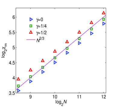
Figure 2: Maximum susceptibility $\chi_{m}$ as a function of system size $N$. We can see that the numerical results approach to the solid line with slope $2/3$ as the system size increases.

Immediately, one can obtain the asymptotic form of all the spin expectation values

$$\frac{2\langle S_{z}\rangle}{N}\bigg{|}_{h=1} \sim 1+\frac{1}{N}+\frac{a_{z}^{\left(0\right)}}{N^{2/3}},$$

$$\frac{4\langle S_{x}^{2}\rangle}{N^{2}}\bigg{|}_{h=1} \sim\frac{a_{xx}^{\left(0\right)}}{N^{2/3}},$$

$$\frac{4\langle S_{y}^{2}\rangle}{N^{2}}\bigg{|}_{h=1} \sim\frac{a_{yy}^{\left(0\right)}}{N^{4/3}},$$

$$\frac{4\langle S_{z}^{2}\rangle}{N^{2}}\bigg{|}_{h=1} \sim 1+\frac{2}{N}+\frac{a_{zz}^{\left(0\right)}}{N^{2/3}}.$$ (36)

where $a_{\xi}^{\left(0\right)}$’s ($\xi=z,xx,yy,zz$) are all constants depending on $\gamma$. Then take the first-order derivatives of Eq. (31) with $h$, one could find similar scaling functions with Eq. (34). Here we also take $2\langle S_{z}\rangle/N$ for example,

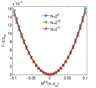
Figure 3: Finite size scaling is performed. The susceptibility $\chi$ is considered as a function of the system size $N$ and the parameter $h$, take the form $N^{\nu}\left(h-h_{m}\right)$. Here the exponent $\nu=2/3$ is determined analytically. It’s noticed that the data dose not collapse at one line exactly since the system sizes are not large enough.

$$\left(\frac{\partial}{\partial h}\frac{2\langle S_{z}\rangle}{N}\right)^{\text{sing}}\simeq\frac{1}{NG\left(h,\gamma\right)^{3/2}}\mathscr{G}_{S_{z}}\left[NG\left(h,\gamma\right)^{3/2},\gamma\right],$$ (37)

where $\mathscr{G}_{\Phi}$ is a scaling function for the derivatives of spin expectation values, and then we find the finite size scaling

$$\frac{\partial}{\partial h}\frac{2\langle S_{z}\rangle}{N}\bigg{|}_{h=1}\sim a_{z}^{\left(1\right)}.$$ (38)

The scaling form of the other derivatives are

$$\frac{\partial}{\partial h}\frac{4\langle S_{x}^{2}\rangle}{N^{2}}\bigg{|}_{h=1} \sim a_{xx}^{\left(1\right)},$$

$$\frac{\partial}{\partial h}\frac{4\langle S_{y}^{2}\rangle}{N^{2}}\bigg{|}_{h=1} \sim\frac{a_{yy}^{\left(1\right)}}{N^{2/3}},$$

$$\frac{\partial}{\partial h}\frac{4\langle S_{z}^{2}\rangle}{N^{2}}\bigg{|}_{h=1} \sim a_{zz}^{\left(1\right)},$$ (39)

where $a_{\xi}^{\left(1\right)}$’s ($\xi=z,xx,yy,zz$) are constants depending on $\gamma$. As we can see that, except for $4\langle S_{y}^{2}\rangle/N^{2}$, the other first-order derivatives are all independent of $N$. Then with the help of Eq. (22), we find that the maximum RFS $\chi_{m}\equiv\chi\left(h_{m},N,\gamma\right)$ is

$$\chi_{m}\sim-\frac{\left(a_{zz}^{\left(1\right)}\right)^{2}N}{a_{zz}^{\left(0\right)}N^{1/3}+2},$$ (40)

for large $N$, and here we just present the divergent term. It’s noticed that $a_{zz}^{\left(0\right)}$ should be less than $-2$ to ensure the matrix element $y>0$, thus $\chi_{m}>0$. Then we have

$$\ln\chi_{m}=A_{N}\ln N+\text{const.}~{},$$ (41)

where the constant only depends on $\gamma$ and the scaling exponent $A_{N}$ approaches to $2/3$ as $N$ increases, which is verified numerically, and $A_{N}=2/3$ in thermodynamic limit. The numerical comparisons are shown in Fig. (2). While in the broken symmetric phase ($0<h<1$), we can derive the same scaling exponents Dusuel and Vidal (2005). However, for global fidelity susceptibility, the scaling exponent is $9/7$ Kwok et al. (2008).

Then if we cancel $N$ in Eq. (37), with similar steps, we can get the relation between the susceptibility $\chi$ and $\eta=h-h_{c}$ in thermodynamic limit,

$$\ln\chi\left(h,\gamma\right)=A_{h}\ln\left|h-h_{c}\right|+\text{const.}~{},$$ (42)

where $A_{h}$ approaches to $-1$ as $h$ goes to $h_{c}$, and the constant depends on $\gamma$. Therefore we could take the form of the susceptibility for finite size as

$$\chi\left(h,N,\gamma\right)=\frac{A}{N^{-2/3}+B\left(h-h_{m}\right)}.$$ (43)

To study the critical behavior around the phase transition point, we could perform the finite scaling analysis. According to the scaling ansatz Barber (1983), the susceptibility is a function of $N^{\nu}\left(h-h_{m}\right)$. In the case of logarithmic divergence, it behaves as $\chi\left(h_{m},N\right)/\chi\left(h,N\right)\sim Q\left[N^{v}\left(h-h_{m}\right)\right]$, where the function $Q(x)\approx\ln x$ for large $x$ is universal and does not depend on system size $N$. Hence with Eqs. (41) and (43), we determine the exponent $v=2/3$, which is confirmed numerically, as shown in Fig. (3). However, the curves for different system sizes does not collapse to a single one exactly, since the system sizes are not large enough. 

IV Conclusion

In summary, we have investigated the RFS in the second order quantum phase transition of the LMG model. For the case that $\rho$ is block-diagonal in $2\times 2$ matrices, we derive a general formula for RFS. Then with the CUTs and the scaling ansatz, the critical exponents, including the finite-size scaling exponents of the RFS are obtained analytically, and confirmed numerically. Our results show that, the RFS undergoes singularity around the critical point, indicating that the RFS can be used to characterize the QPTs. And it’s suggested that we can extract information of the QPTs only from the fidelity of a subsystem, without probing the global system, which is of practical significance in experiments. It is also interesting to study finite-size scaling of RFS in other models such as quantum Ising model, which is under consideration.

V Acknowledgements

We are indebted to Shi-Jian Gu, C. P. Sun and Z. W. Zhou for fruitful and valuable discussions. The work was supported by the Program for New Century Excellent Talents in University (NCET), the NSFC with grant nos. 90503003, the State Key Program for Basic Research of China with grant nos. 2006CB921206, the Specialized Research Fund for the Doctoral Program of Higher Education with grant No.20050335087.

References

- Osterloh et al. (2002) A. Osterloh, L. Amico, G. Falci, and R. Fazio, Nature 416, 608 (2002).
- Vidal et al. (2004a) J. Vidal, G. Palacios, and R. Mosseri, Phys. Rev. A 69, 022107 (2004a).
- Latorre et al. (2005) J. I. Latorre, R. Orus, E. Rico, and J. Vidal, Phys. Rev. A 71, 064101 (2005).
- Barthel et al. (2006) T. Barthel, S. Dusuel, and J. Vidal, Phys. Rev. Lett. 97, 220402 (2006).
- Vidal et al. (2004b) J. Vidal, R. Mosseri, and J. Dukelsky, Phys. Rev. A 69, 054101 (2004b).
- Quan et al. (2006) H. T. Quan, Z. Song, X. F. Liu, P. Zanardi, and C. P. Sun, Phys. Rev. Lett. 96, 140604 (2006).
- Zanardi and Paunković (2006) P. Zanardi and N. Paunković, Phys. Rev. E 74, 031123 (2006).
- Buonsante and Vezzani (2007) P. Buonsante and A. Vezzani, Phys. Rev. Lett. 98, 110601 (2007).
- Zanardi et al. (2007) P. Zanardi, M. Cozzini, and P. Giorda, J. Stat. Mech. 2, L02002 (2007).
- Cozzini et al. (2007) M. Cozzini, P. Giorda, and P. Zanardi, Phys. Rev. B 75, 014439 (2007).
- You et al. (2007) W.-L. You, Y.-W. Li, and S.-J. Gu, Phys. Rev. E 76, 022101 (2007).
- Zhou and Barjaktarevic (2007) H. Q. Zhou and J. P. Barjaktarevic, arXiv:cond-mat/0701608 (2007).
- Zhou et al. (2007) H. Q. Zhou, J. H. Zhao, and B. Li, arXiv:0704.2940 (2007).
- Zhou (2007) H. Q. Zhou, arXiv:0704.2945 (2007).
- Venuti and Zanardi (2007) L. C. Venuti and P. Zanardi, Phys. Rev. Lett. 99, 095701 (2007).
- Gu et al. (2007) S. J. Gu, H. M. Kwok, W. Q. Ning, and H. Q. Lin, arXiv:0706.2495 (2007).
- Chen et al. (2007) S. Chen, L. Wang, S.-J. Gu, and Y. Wang, Phys. Rev. E 76, 061108 (2007).
- Ning et al. (2008) W. Q. Ning, S. J. Gu, C. Q. Wu, and H. Q. Lin, J. Phys.: Condens. Matter 20, 235236 (2008).
- Kwok et al. (2008) H.-M. Kwok, W.-Q. Ning, S.-J. Gu, and H.-Q. Lin, arXiv:0710.2581v1 (2008).
- Yang (2007) M.-F. Yang, Phys. Rev. B 76, 180403 (2007).
- Zhao and Zhou (2008) J.-H. Zhao and H.-Q. Zhou, arXiv:0803.0814 (2008).
- Chen et al. (2008) S. Chen, L. Wang, Y. Hao, and Y. Wang, Phys. Rev. A 77, 032111 (2008).
- Yang et al. (2008) S. Yang, S.-J. Gu, C.-P. Sun, and H.-Q. Lin, arXiv:0803.1292 (2008).
- Gorin et al. (2006) T. Gorin, T. Prosen, T. H. Seligman, and M. Znidaric, Phys. Rep. 435, 33 (2006).
- Paunkovic et al. (2008) N. Paunkovic, P. D. Sacramento, P. Nogueira, V. R. Vieira, and V. K. Dugaev, Phys. Rev. A 77, 052302 (2008).
- Lipkin et al. (1965) H. J. Lipkin, N. Meshkov, and A. J. Glick, Nucl. Phys. 62, 188 (1965).
- Wegner (1994) F. Wegner, Ann. Physik 3, 77 (1994).
- Glazek and Wilson (1993) S. D. Glazek and K. G. Wilson, Phys. Rev. D 48, 5863 (1993).
- Glazek and Wilson (1994) S. D. Glazek and K. G. Wilson, Phys. Rev. D 49, 4214 (1994).
- Uhlmann (1976) A. Uhlmann, Rep. Math. Phys. 9, 272 (1976).
- Botet et al. (1982) R. Botet, R. Jullien, and P. Pfeuty, Phys. Rev. Lett. 49, 478 (1982).
- Botet and Jullien (1983) R. Botet and R. Jullien, Phys. Rev. B 28, 3955 (1983).
- Dusuel and Vidal (2004) S. Dusuel and J. Vidal, Phys. Rev. Lett. 93, 237204 (2004).
- Dusuel and Vidal (2005) S. Dusuel and J. Vidal, Phys. Rev. B 71, 224420 (2005).
- Wang and Mølmer (2002) X. Wang and K. Mølmer, Eur. Phys. J. D 18, 385 (2002).
- Dusuel and Uhrig (2004) S. Dusuel and G. S. Uhrig, J. Phys. A, 9275 37 (2004).
- Barber (1983) M. N. Barber, Phase Transition and Critical Phenomena, vol. 8 (1983).
- guparfide (2008) Ho-Man Kwok and Chun-Sing Ho and Shi-Jian Gu, arXiv:0805.3885 (2008).