Sparse power-efficient topologies for wireless ad hoc sensor networks

Abstract

We study the problem of power-efficient routing for multihop wireless ad hoc sensor networks. The guiding insight of our work is that unlike an ad hoc wireless network, a wireless ad hoc sensor network does not require full connectivity among the nodes. As long as the sensing region is well covered by connected nodes, the network can perform its task. We consider two kinds of geometric random graphs as base interconnection structures: unit disk graphs $\mbox{UDG}(2,\lambda)$ and $k$-nearest-neighbor graphs $\mbox{NN}(2,k)$ built on points generated by a Poisson point process of density $\lambda$ in $\mathbb{R}^{2}$. We provide subgraph constructions for these two models $\mbox{UDG-SENS}(2,\lambda)$ and $\mbox{NN-SENS}(2,k)$ and show that there are values $\lambda_{s}$ and $k_{s}$ above which these constructions have the following good properties: (i) they are sparse; (ii) they are power-efficient in the sense that the graph distance is no more than a constant times the Euclidean distance between any pair of points; (iii) they cover the space well; (iv) the subgraphs can be set up easily using local information at each node. Our analyses proceed by coupling the random graph constructions in $\mathbb{R}^{2}$ with a site percolation process in $\mathbb{Z}^{2}$ and using the properties of the latter to derive properties of the former. An important consequence of our constructions is that they provide new upper bounds for the critical values of the parameters $\lambda$ and $k$ for the models $\mbox{UDG}(2,\lambda)$ and $\mbox{NN}(2,k)$. We also describe a simple local algorithm requiring only location information (from a GPS for example) and communication with immediate neighbors for setting up the subnetworks $\mbox{UDG-SENS}(2,\lambda)$ and $\mbox{NN}(2,k)$ and for routing packets on them.

1 Introduction

Multihop sensor networks, where nodes act not only to sense but also to relay information, have proven advantages in terms of energy efficiency over single hop sensor networks [11]. Not only is sensor-to-sensor communication useful for necessary tasks like time synchronization [6], for certain kinds of collaborative sensing functions like target tracking [23] sensor-to-sensor communication is essential. The question of how to achieve connectivity arises here just as it does in ad hoc wireless networks with one crucial difference:

It is not necessary that every sensor be part of a connected network. It is only necessary that the density of connected sensors is high enough to perform the sensing function.

In other words, even if some sensors are wasted in the sense that the data they sense cannot be relayed, it does not matter as long as the area being sensed is well covered with useful sensors which are part of multihop network that can relay data. The difference from other ad hoc wireless networks is that each node expects connectivity as a service provided to it, while in the WASN individual nodes are not important, the overall task is. In this paper we follow this critical insight to propose sparse easy-to-compute power-efficient constructions for multihop WASNs.

We consider two different types of geometric random graphs as the base interconnection structures. The nodes are modelled by a Poisson point process with density $\lambda$ on the plane, $\mathbb{R}^{2}$. The interconnections between these points are modeled in two ways: 1) Unit Disk Graphs in which there is an edge between two nodes if the Euclidean distance between them is at most 1 and 2) $k$-nearest neighbor graphs in which each node establishes (undirected) edges to the $k$ points nearest to it. We will refer to the former model as $\mbox{UDG}(2,\lambda)$ and the latter as $\mbox{NN}(2,k)$ (following the notation introduced in [8]). The 2 in both these terms denotes the dimension of the space. Both these models display a critical phenomenon. For $\mbox{UDG}(2,\lambda)$ it is known that there is a value $\lambda_{c}^{(2)}$ such that if $\lambda>\lambda^{(2)}_{c}$ the graph contains an infinite component [16]. For $\mbox{NN}(2,k)$ the density is not relevant, instead Haggström and Meester show that $k$ is the critical parameter (see [8]) i.e. there is a $k_{c}(2)$ such that for all $k>k_{c}(2)$, $\mbox{NN}(2,k)$ has an infinite component. We show that as long as the critical parameters take at least certain values (which are higher than the critical values) it is possible in both cases to construct a subgraph of the infinite component with the following properties:

P1. (Sparsity) The subgraph has a maximum degree of 4.

P2. (Constant stretch) The distance between any two points in the subgraph is at most a constant factor greater than the Euclidean distance between the points.

P3. (Coverage) The subgraph is infinite and the probability of a square region of $\mathbb{R}^{2}$ not containing any points of the subgraph decays exponentially with the size of the region.

P4. (Local computability) Each node can determine if it is part of the subgraph by using its location information and by communicating with its immediate neighbours.

The subgraph constructed for $\mbox{UDG}(2,\lambda)$ is called $\mbox{UDG-SENS}(2,\lambda)$ and that constructed for $\mbox{NN}(2,k)$ is called $\mbox{NN-SENS}(2,k)$. We will show that there is a value $\lambda_{s}$ (and $k_{s}$) such that for all $\lambda\geq\lambda_{s}$ (resp. $k\geq k_{s}$), $\mbox{UDG-SENS}(2,\lambda)$ (resp. $\mbox{NN-SENS}(2,k)$) has properties (P1)-(P4). These properties align well with the properties of power-efficient spanners studied in the context of ad hoc wireless networks (see [18, pp 177-178].) The difference being that not every point of the point process is required to be part of the network as long as the sensing function is satisfied (which the coverage property (P3) ensures.).

Property (P2) is of major consequence to the power consumption of the network. This follows from the relationship between the stretch in distance between two points and the consequent increase in the power consumed in communicating between them. Formally, if we consider a wireless network $G$ formed on a set of nodes $V$ in $\mathbb{R}^{2}$, the distance stretch, $\delta$, of a subgraph $H\subseteq G$ is defined as

$$\delta=\max_{u,v\in V}\frac{d_{H}(u,v)}{d_{G}(u,v)},$$

where $d_{G}(u,v)$ is the graph distance between $u$ and $v$ in $G$ i.e. distance between $u$ and $v$ using the edges graph $G$ and $d_{H}(u,v)$ is the graph distance in $H$. Li, Wan and Wang [14, Lemma 2] showed that given a connection network $G$ and a subgraph $H$ with distance stretch $\delta$, the power taken to communicate between any two nodes is at most $\delta^{\beta}$ where $\beta$ is a parameter varying between 2 and 5. Clearly a network with property (P2) achieves a constant power stretch since the Euclidean distance between two points is a lower bound on the distance between them in both $\mbox{UDG}(2,\lambda)$ and $\mbox{NN}(2,k)$. Hence we claim that our constructions are power-efficient up to a constant factor. Additionally we have property (P3) that guarantees coverage of the region being sensed. We show that the probability that a region does not contain a point of $\mbox{UDG-SENS}(2,\lambda)$ (or $\mbox{NN-SENS}(2,k)$) decays exponentially with the size of the region when $\lambda\geq\lambda_{s}$ (respectively $k\geq k_{s}$). In both cases the decay is sharper if a larger value of $\lambda$ is chosen. This allows us to achieve a target coverage by increasing the density to a high enough level.

The basic idea behind our constructions is to couple the random graph in $\mathbb{R}^{2}$ with a discrete site percolation process in $\mathbb{Z}^{2}$. The subgraph we construct mimics the nodes of a percolated mesh. One important byproduct of our constructions is that they give the best known upper bounds on the critical values for both our setting. We improve the best known bound of 213 (due to Teng and Yao [21]) for the critical value of $k$ for $\mbox{NN}(2,k)$ to 188. We also improve the bound for the critical value of $\lambda$ in $\mbox{UDG}(2,\lambda)$ to $1.568$.

The construction is easy to realize using location information (which can be obtained using a GPS) and local computation, hence satisfying property (P4). The algorithm for routing on our subgraph constructions is based on a simple distributed algorithm for routing on the percolated lattice given by Angel et. al. [1].

In the rest of this section we introduce some notation and definitions that will be required. We also discuss the various strands of research relevant to our paper. In Section 2 we describe our constructions $\mbox{UDG-SENS}(2,\lambda)$ and $\mbox{NN}(2,k)$ and give lower bounds on the values $\lambda_{s}$ and $k_{s}$ above which properties (P1)-(P4) hold. The results regarding stretch and coverage are detailed in 3. In Section 4 we discuss the algorithmic issues involved in forming our subgraphs from the underlying structure and also describe how to route packets once the structures are made.

1.1 Preliminaries

We will use the notation $d(x,y)$ to denote the Euclidean distance between two points $x,y\in\mathbb{R}^{2}$. In general we will denote the graph distance (i.e. the shortest path along the edges of the graph) of two vertices $u,v$ of a graph $G$ by $d_{G}(u,v)$. For the random graphs $\mbox{NN}(2,k)$ and $\mbox{UDG}(2,\lambda)$ we will use the notation $d_{n}(u,v)$ and $d_{u}(u,v)$ to denote the graph distance between them.

Poisson point processes

Our random point sets are generated by homogenous Poisson point processes of intensity $\lambda$ in $\mathbb{R}^{2}$. Under this model the number of points in a region is a random variable that depends only on its $d$-dimensional volume i.e. the number of points in a bounded, measurable set $A$ is Poisson distributed with mean $\lambda V(A)$ where $V(A)$ is the $d$-dimensional volume of A. Further, the random variables associated with the number of points in disjoint sets are independent.

Unit disk graphs

The random graph model $\mbox{UDG}(2,\lambda)$ is defined as follows: Given a set of points $S$ generated by a Poisson point process in $\mathbb{R}^{2}$ with density $\lambda$, there is an edge between points $x\in S$ and $y\in S$ if $d(x,y)\leq 1$.

$k$-nearest neighbor graphs

The random graph model $\mbox{NN}(2,k)$ defined as follows: Given a set of points $S$ generated by a Poisson point process in $\mathbb{R}^{2}$ there is an (undirected) edge between points $x\in S$ the $k$ points in $S\setminus\{x\}$ that are closest to $x$. Note that the event that two points have exactly the same distance from a point is a measure 0 event, but for practical purposes we can use any tie-breaking mechanism we deem fit.

Site percolation

Consider an infinite graph defined on the vertex set $\mathbb{Z}^{d}$ with edges between points $x$ and $y$ such that $\|x-y\|_{1}=1$. Site percolation is a probabilistic process on this graph. Each point of $\mathbb{Z}^{d}$ is taken to be open with probability $p$ and closed with probability $1-p$. Hence we have a sample space $\Omega=\prod_{x\in\mathbb{Z}^{d}}\{0,1\}$, individual elements of which are configurations $\omega=(\omega(x):x\in\mathbb{Z}^{d})$. The product of all the measures for individual points forms a measure for the space of possible configurations. An edge between two open vertices is considered open. All other edges are considered closed. A component in which open vertices are connected through paths of open edges is known as an open cluster. It is known that there is a value $p_{c}$ such that for all $p>p_{c}$ the graph obtained has an infinite open cluster. This value is known as the critical probability. When $p>p_{c}$ then each point of $\mathbb{Z}^{d}$ has some non-zero probability of being part of an infinite cluster. The reader is referred to [7] for a full treatment of percolation and to [4] for a recent update on some new directions in this area.

When the lattice undergoes percolation, the path between two connected vertices might become long and tortuous. We introduce some notation for this setting. The distance between two lattice points $x,y\in\mathbb{Z}^{d}$ will be denoted $D(x,y)$. When the lattice has been percoalted with probability $p$, the distance will be denoted $D^{p}(x,y)$. Antal and Pisztora studied this setting and proved a powerful theorem which we state here as a lemma [2, Theorems 1.1 and 1.2]. We adopt the restatement of Angel et. al. [1, Lemma 8].

Lemma 1.1

[2, 1] For any $p>p_{c}$ and any $x,y$ connected through an open path in a cube $M^{d}$ of the infinite lattice. For some $\rho,c_{2}>0$ depending only on the dimension and $p$ and for any $a>\rho\cdot D(x,y)$

$$pr(D^{p}(x,y)>a))<e^{-c_{2}a}.$$

1.2 Related work

Wireless networks

Topology control in wireless networks has been studied extensively (see e.g. the surveys by Santi [18] and Rajaraman [17].) Two important goals of the research in this area have been ensuring connectivity of all nodes and energy-efficiency.

The approach has been to take the underlying topology as a unit disk graph [19] or a proximity graph (for which several proposals exist c.f. surveys cited above) on a point set and then construct some kind of spanning subgraph of this point set with low degree, constant stretch and the property that each node can compute its connections using local information. Although this line of research has the same flavour as our work, it is different in a fundamental way - we do not require all nodes to be connected - and so we do not survey the literature in detail instead referring the reader to general surveys on topology control by and and a specific survey on spanners by Li and Wang [15].

Geometric random graphs and percolation

The study of random graphs obtained by applying connection rules on stationary point processes is known as continuum percolation. Meester and Roy’s monograph on the subject provides an excellent view of the deep theory that has been developed around this general setting [16]. $\mbox{UDG}(2,\lambda)$ is studied in [16], where the existence and non-triviality of the critical density is demonstrated. Kong and Zeh [12] show a lower bound of 0.7698 on $\lambda_{c}$. An upper bound of 3.372 was earlier shown by Hall [9]. Hall’s paper states an upper bound 0.843 for a model of intersecting spheres which scales by a factor of 4 using scaling property of coninumm percolation models [16].

The $\mbox{NN}(d,k)$ model was introduced by Häggström and Meester [8]. They showed that there was a finite critical value, $k_{c}(d)$ for all $d\geq 2$ such that an infinite cluster exists in this model. They proved that the infinite cluster was unique and that there was a value $d_{0}$ such that $k_{c}(d)=2$ for all $d>d_{0}$. Teng and Yao gave an upper bound of 213 for $k_{c}(d)$ [21].

$k$-nearest neighbor graphs on random point sets contained inside a finite region have been extensively studied. The major concern, different from ours, has been to ensure that all the points within the region are connected within the same cluster. Ballister, Bollobás, Sarkar and Walters [3] showed that the smallest value of $k$ that will ensure connectivity lies between $0.3043\log n$ and $0.5139\log n$, improving earlier results of Xue and Kumar [22]. Ballister et. al. also studied the problem of covering the region with the discs containing the $k$-nearest neighbours of the points. We refer the reader to [3] for an interesting discussion relating this setting to earlier work by Penrose and others.

2 The subgraph constructions

In this section we describe our constructions and prove some important properties. We begin by giving a general overview of our technique, then move on to the specifics of the two settings. For both constructions we proceed by viewing $\mathbb{R}^{2}$ as a union of a countably infinite set of square tiles. Inside each tile we look for a two kinds of points. The first kind is what we call a representative point. Representative points lie at the centre of the tile, roughly speaking. We also look for relay points, which help connect representative points to neighbouring tiles. Both these kinds of points have precise definitions that differ for $\mbox{UDG-SENS}(2,\lambda)$ and $\mbox{NN-SENS}(2,k)$, we will discuss those in Section 2.1 and 2.2 respectively. A tile in which we find both kinds of points we call a good tile, other tiles are bad. We connect representative points to four relay points, one for each neighbouring tile. Several points within and outside good tiles may be left unconnected. See Figure 1 for a pictorial depiction. Note that representative points have degree 4 and relay points have degree 2.

Figure 1: A portion of the tiling of $\mathbb{R}^{2}$.

The subgraph drawn by connecting representative points through relay points will be the network we will use for sensing. In order to prove properties (P1)-(P4) we will couple the tiling with a site percolation process in $\mathbb{Z}^{2}$. We associate each tile in $\mathbb{R}^{2}$ with a point in $\mathbb{Z}^{2}$. We declare a site in $\mathbb{Z}^{2}$ open only if the tile corresponding to it in $\mathbb{R}^{2}$ is good. Hence the probability that a site is open is equal to the probability that its corresponding tile is good. Our definitions of representative and relay points will ensure that if two neighbouring tiles are good then their representative points are connected through their relay points as shown in Figure 2. This corresponds to the edge between two open sites being open in $\mathbb{Z}^{2}$ (see Figure 2.)

Figure 2: The part of $\mathbb{Z}^{2}$ corresponding to the tiles shown in Figure 1.

Since paths in $\mathbb{Z}^{2}$ corresponds to paths between points in $\mathbb{R}^{2}$ it follows that if percolation occurs in the $\mathbb{Z}^{2}$ then an infinite component must exist in the geometric random graph model as well. Hence we can conclude that if the probability of a tile being good exceeds the critical probability for site percolation, the geometric random graph model also has an infinite component in it almost surely. Let us now take a more specific look at the constructions for $\mbox{UDG}(2,\lambda)$ and $\mbox{NN}(2,k)$.

2.1 Unit-disk graphs

The internal structure of a tile for the construction of $\mbox{UDG-SENS}(2,\lambda)$ is shown in Figure 3.

Figure 3: A tile $t$ and it’s 5 relevant regions. Note that the region $E_{r}$ is the part of the intersection lying wholly within $t$ of all unit discs centred at points in $C_{0}$ and in the region $E_{l}$ (i.e. the left relay region) of the neighbour tile $t_{r}$.

We consider square tiles of side 4/3. For the sake of exposition let us assume that the tile shown in Figure 3 is centred at (0,0) and it’s lower left corner is (-2/3, -2/3). Within each tile we consider five disjoint regions, the representative region $C_{0}(t)$, and the relay regions $E_{l}(t),E_{r}(t),E_{t}(t)$ and $E_{b}(t)$. $C_{0}(t)$ is a circle of radius 1/2 centred at the origin. The regions $E_{i}(t),i\in\{l,r,t,b\}$ are intuitive to understand but slightly tricky to describe formally. We describe one of them, $E_{r}(t)$. In order to do so, let us denote by $t_{r}$ the tile immediately to the right of the tile $t$ i.e. the tile centred at (4/3,0) with bottom left corner (2/3,-2/3). It’s leftmost relay region is $E_{l}(t_{r})$. Now we define $E_{r}(t)$ as the part of the intersection lying wholly within $t$ of all circles of unit radius centred at points in $C_{0}(t)$ and $E_{l}(t_{r})$. From this set we remove all the points of $C_{0}(t)$. In the figure the region is depicted by an ellipse, but clearly it is a less regular shape.

We call a tile $t$ good if each of $C_{0}(t)$ and $E_{i}(t),t\in\{l,r,b,t\}$ contains at least one point of the point process. One of the points contained in $C_{0}(t)$ will be the representative point for this tile, denoted $\mbox{rep}(t)$. Four other points, one from each of the regions $E_{i}(t),t\in\{l,r,b,t\}$ will be the relay points for this good tile. If a region has more than one point, the tie has to be broken. This will be done in a distributed fashion. We postpone the discussion of this aspect to Section 4. Note that some of the relay regions overlap and hence it may be the case that one point fulfils two relay functions.

According to the program described earlier we create a bijection, $\phi$, between the tiles in $\mathbb{R}^{2}$ and points in $\mathbb{Z}^{2}$ such that neighbouring tiles in $\mathbb{R}^{2}$ correspond to neighbouring points in $\mathbb{Z}^{2}$. We couple $\mbox{UDG}(2,\lambda)$ to a site percolation process in $\mathbb{Z}^{2}$ by saying that a given point $x$ in $\mathbb{Z}^{2}$ is open only if the tile $t=\phi^{-1}(x)$ is good. Now we can claim that the existence of an edge in $\mathbb{Z}^{2}$ implies the existence of a path from the representative points of the two tiles corresponding to the two end points of the edge. We state this formally, including an observation about the distance stretch between the two representative points.

Claim 2.1

If an edge exists in the percolated mesh $\mathbb{Z}^{2}$ between two points $x$ and $y$ then

1. There is a path between the representative points $\mbox{rep}(\phi^{-1}(x))$ and $\mbox{rep}(\phi^{-1}(y))$ of the tiles corresponding to $x$ and $y$ in $\mbox{UDG}(2,\lambda)$ and

2. there is a constant $c_{\mbox{u}}\leq 3$ such that

   $$d_{k}(\mbox{rep}(\phi^{-1}(x)),\mbox{rep}(\phi^{-1}(y)))\\ \leq c_{\mbox{u}}\cdot d(\mbox{rep}(\phi^{-1}(x)),\mbox{rep}(\phi^{-1}(y))).$$ (1)

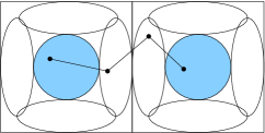
Figure 4: A path between the representative points of neighboring good tiles.

Proof.  Clearly if two neighbouring tiles $t$ and $t^{\prime}$ are good, by the goodness condition there will be an edge from the representative point of one of them to a relay point in the direction of its neighbor. This relay point will subsequently connect to the relay point of that neighbor closest to it, which will in turn be connected to the representative point of the neighbour (see Figure 4). Clearly each of the three edges on the path from $\mbox{rep}(t)$ to $\mbox{rep}(t^{\prime})$ is at most 1 unit in length so $c_{\mbox{u}}\leq 3$. $\sqcap$$\sqcup$

The largest connected component formed by the representative points and relay points is $\mbox{UDG-SENS}(2,\lambda)$.

From Claim 2.1, it is easy to deduce that if an infinite component exists in the site percolation setting, then an infinite component exists in $\mbox{UDG}(2,\lambda)$. Hence we need to determine for what values of $\lambda$ the site percolation process is supercritical. The critical probability for site percolation lies between 0.592 and 0.593 (see e.g. [13]). Numerical calculations showed that the smallest value of $\lambda$ for which the probability of a tile being good exceeds 0.593 is $\lambda_{s}=1.568$. Hence for $\lambda$ larger than this value $\mbox{UDG-SENS}(2,\lambda)$ is infinite.

Since this improves the best known upper bound of 3.372 [12], we state it here as a theorem.

Theorem 2.2

For $\mbox{UDG}(2,\lambda)$

$$\lambda^{(2)}_{c}<1.568.$$

In Section 3 we will show that $\mbox{UDG-SENS}(2,\lambda)$ for $\lambda\geq\lambda_{s}$ has constant stretch. For now we move on to the construction of $\mbox{NN-SENS}(2,k)$.

2.2 Nearest-neighbor graphs

The internal structure of a tile for the construction of $\mbox{NN-SENS}(2,k)$ is shown in Figure 5.

Figure 5: A tile $t$ and it’s 9 relevant regions. Note that the region $E_{r}$ lies wholly within all discs of the form $C_{x}$ and $C_{z}$ centred at points on the boundary of the discs $C_{0}$ and $C_{r}$.

Let us say that the tile in Figure 5 is centred at $(0,0)$ with bottom left corner $(-5a,-5a)$ and top right corner $(5a,5a)$. For convenience we will refer to the tiles surrounding the tile $t$ as, couunterclockwise starting from the right $t_{r}$, $t_{t}$, $t_{l}$ and $t_{b}$. We consider five circles of radius $a$: $C_{0}$ centred at $(0,0)$, $C_{l}$ centred at $(-4a,0)$, $C_{r}$ centred at $(4a,0)$, $C_{t}$ centred at $(0,4a)$ and $C_{b}$ centred at $(0,-4a)$. There are four other region which are named $E_{l},E_{r},E_{t}$ and $E_{b}$ in the figure. $E_{r}$ is defined as follows. Consider the largest circle centred at any point in $C_{0}$ or $C_{r}$ that lies wholly within the two tiles $t$ and $t_{r}$. Two such circles, $C_{x}$ and $C_{z}$, are depicted in Figure 5. $E_{r}$ is the locus of the points contained in all such circles. The regions $E_{l},E_{t}$ and $E_{b}$ are defined similary by $C_{0}$ alongwith $C_{l},C_{t}$ and $C_{b}$ respectively and the tiles $t_{l},t_{t}$ and $t_{b}$ respectively.

Now, we call tile $t$ good if

1. the number of points inside $t$ is at most $k/2$ and

2. the nine regions $C_{0},C_{r},C_{t},C_{l},C_{b},E_{r},E_{t},E_{l}$ and $E_{b}$ contain at least one point each.

One point contained in $C_{0}$ will be the representative point of the tile $t$, denoted $\mbox{rep}(t)$. A point from each of the other 8 regions will be relay points. If these regions contain multiple points we will have to select one from each and discard the rest. As in the case of $\mbox{UDG-SENS}(2,\lambda)$ we postpone the discussion of how to select this one point each to Section 4.

According to the program described earlier we create a bijection, $\phi$, between the tiles in $\mathbb{R}^{2}$ and points in $\mathbb{Z}^{2}$ such that neighbouring tiles in $\mathbb{R}^{2}$ correspond to neighbouring points in $\mathbb{Z}^{2}$. We couple $\mbox{NN}(2,k)$ to a site percolation process is $\mathbb{Z}^{2}$ by saying that a given point $x$ in $\mathbb{Z}^{2}$ is open only if the tile $t=\phi^{-1}(x)$ is good. Now we can claim that the existence of an edge in $\mathbb{Z}^{2}$ implies the existence of a path from the representative points of the two tiles corresponding to the two end points of the edge. We state this formally, including an observation about the distance stretch between the two representative points.

Claim 2.3

If an edge exists in the percolated mesh $\mathbb{Z}^{2}$ between two points $x$ and $y$ then

1. There is a path between the representative points $\mbox{rep}(\phi^{-1}(x))$ and $\mbox{rep}(\phi^{-1}(y))$ of the tiles corresponding to $x$ and $y$ in $\mbox{NN}(2,k)$ and

2. there is a constant $c_{\mbox{k}}$ such that

   $$d_{k}(\mbox{rep}(\phi^{-1}(x)),\mbox{rep}(\phi^{-1}(y)))\\ \leq c_{\mbox{k}}\cdot d(\mbox{rep}(\phi^{-1}(x)),\mbox{rep}(\phi^{-1}(y))).$$ (2)

\begin{picture}(7823.0,3923.0)(2427.0,-4310.0)\end{picture}

Figure 6: A path between the representative points of two neighboring good tiles.

Proof.  The proof of the claim is depicted in Figure 6 Clearly any circle drawn from $\mbox{rep}(t)$ that stays within $t$ contains all of $E_{r}$ in it by the definition of $E_{r}$. Since there are at most $k/2$ points in every good tile, hence there is an edge from $\mbox{rep}(t)$ to the point guaranteed to be contained in $E_{r}$, let’s call it $x_{r}$. We do not make any claims on where the edges established by $x_{r}$ to its neighbours lie, observing only that any point that lies in $C_{r}$ must have an edge to $x_{r}$, again by the definition of $E_{r}$. However, any disc centred at a point in $C_{r}$ that remains within $t$ and $t_{r}$ must contain the left disc of its neighboring tile. Hence, if $t$ and $t_{r}$ are both good then a path from $\mbox{rep}(t)$ to $\mbox{rep}(t_{r})$ occurs. The second part of the claim is obviously true. The constant $c_{\mbox{k}}$ can easily be calculated using calculus. $\sqcap$$\sqcup$

We define $\mbox{NN-SENS}(2,k)$ as the largest connected component of the graph built on representative and relay points. Note that unlike $\mbox{UDG-SENS}(2,\lambda)$ there are 8 relay points within each tile here and the path between two representative points contains 4 relay points. Also note that only the regions $E_{l},E_{r},E_{t}$ or $E_{b}$ can share relay points. The regions $C_{l},C_{r},C_{t}$ and $C_{b}$ do not intersect in any way. Each of the regions may contain more than one point of the point process. In this case one point has to be be chosen as a representative or relay as the case may be. This can be easily achieved by running a simple leader election algorithm [20] between the nodes in the region which are all connected to each other in any case. We will discuss this issue further in Section 4.

From Claim 2.3, it is easy to deduce that if an infinite component exists in the site percolation setting, then an infinite component exists in $\mbox{NN}(2,k)$. Hence we need to determine for what settings of our parameters $a$ and, more importantly, $k$, the site percolation process is supercritical. The critical probability for site percolation lies between 0.592 and 0.593 (see e.g. [13]). Numerical calculations showed that the smallest value of $k$ for which the probability of a tile being good exceeds 0.593 is 188, and the value of $a$ for which this happens is 0.893.

Like Häggström and Meester’s proof for the existence of a critical value [8] and Teng and Yao’s proof for the weaker of their two upper bounds on $k_{c}(2)$ [21] our proof of Theorem 2.4 proceeds by constructing a coupling with a site percolation process on $\mathbb{Z}^{2}$. However, our construction gives a better upper bound than Teng and Yao’s improvement of their own result (also in [21]) to $k_{c}(2)\geq 213$ which uses a coupling to a mixed percolation process. Hence we state this result as a theorem:

Theorem 2.4

For $\mbox{NN}(2,k)$,

$$k_{c}(2)\leq 188.$$

Having described the constructions of $\mbox{UDG-SENS}(2,\lambda)$ and $\mbox{NN-SENS}(2,k)$ and having shown that there are values of the critical parameters for which these constructions exist, let us now proceed to show that these constructions indeed have constant stretch.

3 Stretch and coverage

In this section we prove that our constructions have constant stretch with high probability when the critical parameters have high enough values. We also show that the coverage of our constructions is very good in a probabilistic sense.

3.1 Constant stretch

The argument for constant stretch of both $\mbox{NN-SENS}(2,k),k\geq k_{s}$ and $\mbox{UDG-SENS}(2,\lambda),\lambda\geq\lambda_{s}$ follow similar lines so we present them together. For the purposes of this section we denote the tile lengths chosen for the two constructions as $a_{u}$ (= 4/3) and $a_{k}$ (= 0.893). In what follows, all arguments hold for both settings except where explicitly noted otherwise. Also in the following we implicitly assume that $k\geq k_{s}$ and $\lambda\geq\lambda_{s}$.

Let us consider any two tiles $t_{1}$ and $t_{2}$ whose representative points $\mbox{rep}(t_{1})$ and $\mbox{rep}(t_{2})$ lie $\mbox{UDG-SENS}(2,\lambda)$ or $\mbox{NN-SENS}(2,k)$. First we relate the distance in the (unpercolated) lattice to the euclidean distance between these two points by observing a simple fact.

Fact 3.1

Given the constants $c_{\mbox{u}}$ defined in Claim 2.1 and $c_{\mbox{k}}$ defined in Claim 2.1, then for two tiles $t_{1},t_{2}$

$$D(\phi(\mbox{rep}(t_{1})),\phi(\mbox{rep}(t_{2})))\leq\sqrt{2a}\cdot\frac{d(\mbox{rep}(t_{1}),\mbox{rep}(t_{2}))}{c}$$

where $c\in\{c_{\mbox{u}},c_{\mbox{k}}\}$ and $a\in\{a_{u},a_{k}\}$ respectively.

Fact 3.1 along with Lemma 1.1 gives us the following theorem:

Theorem 3.2

1. For $\mbox{UDG-SENS}(2,\lambda)$, with $\lambda\geq 1.568$ there are constants $\alpha$ and $c_{1}$ depending only on $\lambda$ such that

   $$\mbox{P}(d_{u}(x,y)>\alpha\cdot D(x,y))<e^{-c_{1}\cdot D(x,y)}.$$

2. For $\mbox{NN-SENS}(2,k)$, with $k\geq 188$ there are constants $\beta$ and $c_{2}$ depending only on $k$ such that

   $$\mbox{P}(d_{k}(x,y)>\beta\cdot D(x,y))<e^{-c_{2}\cdot D(x,y)}.$$

Theorem 3.2 is an existential result. In Section 4 we will show how to actually find the constant stretch paths in a distributed way with bounded overhead. For now we proceed to show that our constructions have good coverage.

3.2 Coverage

Let us consider a square region of size $\ell\times\ell$. Let us call this $B(\ell)$. We will argue that the probability that $B(\ell)$ contains no point of $\mbox{UDG-SENS}(2,\lambda)$ (or $\mbox{NN-SENS}(2,k)$) decays exponentially with $\ell$. As before the arguments here also apply to both the models. We claim the following theorem:

Theorem 3.3

1. For $\lambda\geq 1.568$ there are constants $c_{3},c_{4}$ depending only on $\lambda$ such that

   $$\mbox{P}[|B(\ell)\cap\mbox{UDG-SENS}(2,\lambda)|=0]\leq c_{4}\cdot\ell^{2}\cdot e^{-c_{3}\cdot\ell}.$$

2. For $k\geq 188$ there are constants $c_{5},c_{6}$ depending only on $k$ such that

   $$\mbox{P}[|B(\ell)\cap\mbox{NN-SENS}(2,k)|=0]\leq c_{5}\cdot\ell^{2}\cdot e^{-c_{6}\cdot\ell}.$$

Let us denote by $TB(\ell)$ the set of tiles fully or partially contained in the $B(\ell)$. Let us consider the set $\phi(TB(\ell))$ i.e. the set of all points in $\mathbb{Z}^{2}$ which are images of the tiles in $TB(\ell)$ under the mapping defined earlier. For $B(\ell)\cap\mbox{UDG-SENS}(2,\lambda)$ to be empty, each point of $\phi(TB(\ell))$ must be outside the infinite cluster of the supercritical percolation process. With this insight we now refer the reader to Theorems 8.18 and 8.21 of [7] dealing with the radius of finite clusters in the supercritical phase. A slight modification of the proof of Theorem 8.21 of (due to [5]) will yield the the proof of Theorem 3.3. The details are tedious and do not add anything to the proof described in [7] so we omit them here. Theorem 3.3 yields the following simple corollary

Corollary 3.4

1. There is a constant $c_{7}$ such that for $\ell\geq c_{7}\log n$

   $$\mbox{P}[|B(\ell)\cap\mbox{UDG-SENS}(2,\lambda)|=0]<\frac{1}{n}.$$

2. There is a constant $c_{8}$ such that for $\ell\geq c_{8}\log n$

   $$\mbox{P}[|B(\ell)\cap\mbox{NN-SENS}(2,k)|=0]<\frac{1}{n}.$$

The constants $c_{7}$ and $c_{8}$ may be larger than what the network requires for its sensing function. It seems intuitive that adding more nodes should decrease the values of these constants, but the statement of Theorem 3.3 does not seem to provide this. However we claim this intuition is indeed satisfied for $\mbox{UDG-SENS}(2,\lambda)$ and $\mbox{NN-SENS}(2,k)$. In order to use Theorem 3.3 to provide a guarantee of desired coverage, we argue that the exponential decay indeed grows sharper when the density $\lambda$ increases. This is true for both $\mbox{UDG-SENS}(2,\lambda)$ and $\mbox{NN-SENS}(2,k)$.

For the case of $\mbox{UDG-SENS}(2,\lambda)$ it is not hard to see, since an increase in $\lambda$ directly leads to an increase in the probability of a tile being good. This, through the coupling, increases the probability of the corresponding site in $\mathbb{Z}^{2}$ being open. In the site percolation setting the probability of a site being part of the infinite cluster, $\theta(p)$ is known to increase montonically with the probability $p$ of sites being open. Our claim follows because the increase in $\theta(p)$ is centrally involved in the (omitted) proof of Theorem 3.3. The claim has a slightly subtler provenance for $\mbox{NN-SENS}(2,k)$. Essentially the argument is that if we fix some value $k\geq k_{s}$, increasing the density $\lambda$ allows us to use tiles of smaller side length and still achieve the desired probability ($>p_{c}$) of a tile being good. This implies that the number of tiles within a region increases, and hence the exponential decrease becomes sharper.

4 Algorithmic issues

We now focus on the algorithmic issues involved in building $\mbox{UDG-SENS}(2,\lambda)$ and $\mbox{NN}(2,k)$ and routing packets in them once they are built.

4.1 Forming the networks

After the nodes are laid out in their positions they have to undertake four basic steps. Firstly, they have to identify which tile they belong to. This involves using their location information (assumed to be of the form $(x,y)\in\mathbb{R}^{2}$) and the value of the tile width (denoted $a_{u}$ for $\mbox{UDG-SENS}(2,\lambda)$ and $a_{k}$ for $\mbox{NN-SENS}(2,k)$) programmed into the nodes. In the second step each node determines whether it belongs to one of the special regions within the tile as described in Section 2. In the third step all the nodes within a region communicate to elect a leader who is then designated as the representative point of the tile or a relay point, as applicable. In the fourth step the elected points of each region form connections with the leaders of their neighbouring regions. See Figure 7 for a formal statement of the algorithm for building $\mbox{UDG-SENS}(2,\lambda)$. The algorithm for $\mbox{NN-SENS}(2,k)$ is very similar.

Algorithm construct($\mbox{UDG-SENS}(2,\lambda),a$) 1. At each node $v$ do (a) Determine $(\mbox{\sf location}_{v}(x),\mbox{\sf location}_{v}(y))$. (b) compute $\mbox{\sf id}_{v}(x)=\mbox{\sf location}_{v}(x)/a_{u}$ (c) compute $\mbox{\sf id}_{v}(y)=\mbox{\sf location}_{v}(y)/a_{u}$ (d) compute $\mbox{\sf region}_{v}$ 2. For each tile $t$ and each region $r\in\{C_{0}(t),E_{r}(t),E_{l}(t),E_{t}(t),E_{b}(t)\}$ do (a) Build $S(r,t)=\{v\in t\ |\ \mbox{\sf region}_{v}=r\}$. (b) $\mbox{rep}(t)\leftarrow$ electLeader$(S(C_{0},t))$ (c) For $r\in\{E_{r}(t),E_{l}(t),E_{t}(t),E_{b}(t)\}$
$\mbox{relay}(t,r)\leftarrow$ electLeader$(S(r,t))$ 3. For each tile $t$ with neighbours $t_{l},t_{r},t_{t},t_{b}$ do (a) For each $r\in\{E_{r}(t),E_{l}(t),E_{t}(t),E_{b}(t)\}$
connect$(\mbox{rep}(t),\mbox{relay}(t,r))$. (b) connect$(\mbox{relay}(t,E_{r}(t)),\mbox{relay}(t,E_{l}(t_{r}))$. (c) connect$(\mbox{relay}(t,E_{l}(t)),\mbox{relay}(t,E_{r}(t_{l}))$. (d) connect$(\mbox{relay}(t,E_{t}(t)),\mbox{relay}(t,E_{b}(t_{t}))$. (e) connect$(\mbox{relay}(t,E_{b}(t)),\mbox{relay}(t,E_{t}(t_{b}))$.

Figure 7: Building $\mbox{UDG-SENS}(2,\lambda)$.

The function electLeader can be realized using any distributed leader election algorithm on a complete graph topology since all the nodes within a region can talk to each other (see e.g. [20]. The function named connect is simply a handshake between the two nodes mentioned. Once the calls to this function are over the set up phase is completed.

Note that the algorithm of Figure 7 will not just form the largest component but will also form other small components. It is possible to detect how large a given component is by attempting to send packets to distant nodes. The nodes of a small component can then turn themselves off if they realize they are not part of $\mbox{UDG-SENS}(2,\lambda)$. Detecting connectivity is an area of research in itself so we do not address the issues here, refering the reader to some recent work in this area [10].

4.2 The routing algorithm

For routing purposes the representative points of a tile act as if they are open lattice points in $\mathbb{Z}^{2}$. They use relay points to send packets to the representative points of their neighbouring good tiles (see Figure 8) hence realizing open edges in $\mathbb{Z}^{2}$. With this simple idea in place, we can just plug in any algorithm which performs routing in the percolated mesh.

\begin{picture}(5935.0,5935.0)(2171.0,-6591.0)\end{picture}

Figure 8: The path between two representative points mimics the path in $\mathbb{Z}^{2}$ using relay points to realize edges.

We rely on the algorithm for efficient distributed routing in the giant component of a percolated mesh given by Angel et. al. [1]. Their algorithm proceeds by trying to follow a shortest path from source to destination. If at any point the path is broken (i.e. one of the nodes is closed) they try to find the next node along the path that is open by performing a distributed BFS from the current location of the packet. For our purposes we assume that the canonical shortest path between any two nodes $(x_{1},y_{1}),(x_{2},y_{2})\in\mathbb{Z}^{2}$ is the $x-y$ path: the path that proceeds to first fix the $x$ coordinate then the $y$ coordinate i.e. $(x_{1},y_{1})\rightarrow(x_{2},y_{1})\rightarrow(x_{2},y_{2})$. We describe the routing algorithm in Figure 9.

Algorithm routing($\mbox{rep}(t_{1}),\mbox{rep}(t_{2})$) 1. $\mbox{\sf id}_{s}\leftarrow\mbox{\sf id}_{\mbox{rep}(t_{1})}$. 2. $\mbox{\sf id}_{t}\leftarrow\mbox{\sf id}_{\mbox{rep}(t_{2})}$. 3. $curr\leftarrow\mbox{\sf id}_{s}$. 4. While $curr\neq\mbox{\sf id}_{t}$ do (a) $next\leftarrow$ computeNext($curr,\mbox{\sf id}_{t}$) (b) if isOpen($next$) i. sendTo($next$) ii. $curr\leftarrow next$ else i. run distBFS($curr,\mbox{\sf id}_{t}$) until $v$ lying on the $x-y$ path from $curr$ to $\mbox{\sf id}_{t}$ is found. ii. sendToNode($v$). iii. $curr\leftarrow v$.

Figure 9: Routing packets between the representative points of two tiles.

The function computeNext mentioned in Figure 9 finds the next node along the $x-y$ path. The function isOpen involves checking if the next tile along the path is good or not. This can be done by asking the relevant relay if it has a neighbour in the target tile. The function sendTo uses the relays to pass the packet to the representative node of the next tile which then continues the routing process. This is the simple part of the algorithm. If the target tile is not good a BFS is launched to find the next good tile along the $x-y$ path. This is a distributed algorithm that requires nodes to be probed as the search proceeds. Finally when it finds the destination it has to also report the path back to the node that launched the search. Once this path is known the function sendToNode sends the packet along this path to the discovered node. We refer the reader to Angel et. al. [1] for a proof that the expected number of probes required for this algorithm is at most a constant times the length of the shortest path.

5 Conclusion

In this paper we have shown that it is possible to construct sparse power-efficient wireless ad hoc sensor networks with good coverage if we are willing to accept a certain level of redundancy in the system. Ideas from percolation theory have been used to demonstrate that the infinite cluster of two kinds of geometric random graphs contains a good subgraph with the properties that we seek and that this subgraph can be built efficiently using only local information. It is our conjecture that the subgraphs we build should exist whenever an infinite cluster exists in the geometric random graphs we study. One major direction for future research involves resolving this conjecture one way or the other. Even if this conjecture is not true, it should be possible to bring the values of $k_{s}$ and $\lambda_{s}$ closer to the critical values $\lambda^{(2)}_{c}$ and $k_{c}(2)$.

References

- [1] O. Angel, I. Benjamini, E. Ofek, and U. Wieder. Routing complexity of faulty networks. In Proc. of 24th Annu. ACM Symp.on Principles of Distributed Computing (PODC 2005), pages 209–217, 2005.
- [2] P. Antal and A. Pisztora. On the chemical distance for supercritical Bernuolli percolation. Ann. Probab., 24(2):1036–1048, 1996.
- [3] P. Ballister, B. Bollobás, A. Sarkar, and M. Walters. Connectivity of random -nearest-neighbour graphs. Adv. Appl. Prob. (SGSA), 37:1–24, 2005.
- [4] B. Bollobás and O. Riordan. Percolation. Cambridge University Press, 2006.
- [5] J. T. Chayes, L. Chayes, and C. M. Newman. Bernuolli percolation above threshold: an invasion percolation analysis. Ann. Probab., 15:1272–1287, 1987.
- [6] J. V. Greunen and J. M. Rabaey. Lightweight time synchronization in sensor networks. In Proc. 2nd ACM Intl. Conf. on Wireless Sensor Networks and Applications (WSNA 2003), pages 11–19, 2003.
- [7] G. Grimmett. Percolation, volume 321 of Grundlehren der mathematischen Wissenschaften. Springer, 2nd edition, 1999.
- [8] O. Häggström and R. Meester. Nearest neighbor and hard sphere models in continuum percolation. Random Struct. Algor., 9(3):295–315, 1996.
- [9] P. Hall. On continuum percolation. Ann. Probab., 13(4):1250–1266, 1985.
- [10] M. Jorgic, N. Goel, K. Kalaichevan, A. Nayak, and I. Stojmenovic. Localized detection of k-connectivity in wireless ad hoc, actuator and sensor networks. In Proc. 16th Intl. Conf. on Computer Communications and Networks (ICCCN ’07), pages 33–38, 2007.
- [11] H. Karl and A. Willig. Protocols and Architectures for wireless sensor networks. John Wiley and Sons, 2005.
- [12] Z. Kong and E. M. Yeh. Connectivity and latency in large-scale wireless networks with unreliable links. In Proc. 27th Conf. on Computer Communications (INFOCOM 2008), pages 394–402, 2008.
- [13] M. J. Lee. Complementary algorithms for graphs and percolation. arXiv:0708.0600v1, 2007.
- [14] X.-Y. Li, P.-J. Wan, and Y. Wang. Power efficient and sparse spanner for wireless ad hoc networks. In Proc. 10th Intl. Conf. on Computer Communications and Networks, pages 564–567, 2001.
- [15] X.-Y. Li and Y. Wang. Geometrical spanner for wireless ad hoc networks, chapter 68. Chapman and Hall/CRC, 2007.
- [16] R. Meester and R. Roy. Continuum Percolation. Number 119 in Cambridge Tracts in Mathematics. Cambridge University Press, 1996.
- [17] R. Rajaraman. Topology control and routing in ad hoc networks: A survey. SIGACT News, 33:60–73, June 2002.
- [18] P. Santi. Topology control in wireless ad hoc and sensor networks. ACM Comput. Surv., 37(2):164–914, 2005.
- [19] A. Sen and M. L. Huson. A new model for scheduling packet radio networks. Wirel. Netw., pages 71–82, 1997.
- [20] G. Singh. Leader election in complete networks. In Proc. 11th Annual Symp. on Principle of Distributed Computing (PODC ’92), pages 179–190, 1992.
- [21] S.-H. Teng and F. F. Yao. -nearest-neighbor clustering and percolation theory. Algorithmica, 49:192–211, 2007.
- [22] F. Xue and P. R. Kumar. The number of neighbours needed for the connectivity of wireless networks. Wirel. Netw., 10:169–181, 2004.
- [23] F. Zhao, J. Liu, L. Guibas, and J. Reich. Collaborative signal and information processing: An information directed approach. Proc. IEEE, 32(1):61–72, 2003.