Multiple parton scattering in nuclei: gauge invariance

Abstract

Within the framework of a generalized collinear factorization for multiple parton scattering in nuclear medium, twist-4 contributions to DIS off a large nucleus can be factorized as a convolution of hard parts and two-parton correlation functions. The hard parts for the quark scattering in the light-cone gauge correspond to interaction with a transverse (physical) gluon in the target, while they are given by the second derivative of the cross section with a longitudinal gluon in the covariant gauge. We provide a general proof of the equivalence of the hard parts in the light-cone and covariant gauge. We further demonstrate the equivalence in calculations of twist-4 contributions to semi-inclusive cross section of DIS in both lowest order and next leading order. Calculations of the nuclear transverse momentum broadening of the struck quark in the light-cone and covariant gauge are also discussed.

LBNL-

, and

1 Introduction

In the study of nuclear matter and quark-gluon plasma in high energy lepton-nucleus, hadron-nucleus and nucleus-nucleus collisions, hard processes such as jet and high transverse momentum hadrons production are useful tools as their initial production rates can be calculated within perturbative QCD (pQCD). Modification of the final jet or hadron spectra known as jet quenching [1] due to further interaction between the energetic partons and the nuclear or hot medium can be used to probe the properties of medium such as parton correlation or gluon density [2]. Indeed, strong jet quenching has been observed both in high-energy lepton-nucleus [3] and nucleus-nucleus collisions [4, 5].

Current phenomenological studies of experimental data on jet quenching to extract properties of the nuclear matter or hot medium rely on pQCD calculations of the parton energy loss or modification of the parton fragmentation functions due to gluon radiation induced by multiple scattering during the parton propagation. Among many theoretical studies [6, 7], twist expansion approach [8, 9] was applied to medium modification of the fragmentation functions and parton energy loss in both nuclei in deeply inelastic scattering (DIS) and hot QCD matter in heavy-ion collisions. Such an approach is based on the generalized factorization framework for multiple parton scattering in nuclear medium first developed by Luo, Qiu and Sterman (LQS) [10]. Within this framework, LQS proved that the leading twist-4 contribution from multiple parton scattering in a large nucleus can be factorized as a convolution of hard parts and two-parton correlation functions. Such parton correlation functions have leading contributions that are proportional to the nuclear size $R_{A}\sim A^{1/3}$ and therefore the twist-4 contributions are enhanced by the nuclear medium as compared to the same contribution in nucleon collisions.

The twist expansion technique has been used to calculate the effect of multiple parton scattering in dijet and photon production in DIS off nuclear targets [11, 12] and Drell-Yan (DY) dilepton spectra in $p+A$ collisions [13, 14]. In these calculations, processes involving secondary scattering with a soft gluon (soft scattering) are treated in the framework of collinear expansion in a covariant gauge while processes of secondary scattering with a hard gluon (double hard scattering) are calculated directly in the light-cone gauge with collinear approximation (neglecting the transverse momentum of the initial gluons from the nucleus). In such separate treatments of soft and double hard scattering, it is difficult to include the interference between the two type of processes. For large values of the final transverse momentum of the dijets, photons or DY dilepton, one nevertheless can neglect the interference effects since the formation time of the particle production, which dictates the interference, is much smaller than the nuclear size. In the investigation of nuclear modification of parton fragmentation functions and induced parton energy loss [8, 9], it is critical to consider soft gluon bremsstrahlung. Since the formation time of soft gluons can be larger or comparable to the nuclear size, one has to include the interference between soft and double hard scattering which is equivalent to the Landau-Pomeranchuck-Migdal (LPM) interference [15]. In this case, both soft and double hard processes and their interference terms should be calculated within the general framework of collinear expansion in the same gauge.

In a covariant gauge, the longitudinal component of the gauge field $A^{+}$ is considered large. One usually makes a collinear expansion of the hard part of quark and (longitudinal) gluon interaction. These hard parts do not correspond to any physical quark-gluon scattering. If one expands the hard parts in the transverse momentum of the longitudinal gluon field, the collinear terms are directly related to the hard parts of the vacuum diagram without final gluon interaction. They only contribute to the gauge link of the initial quark distribution function of the vacuum diagram. The higher order terms in the collinear expansion will contribute to higher twist cross section involving two-parton correlation functions and derivatives of the corresponding hard parts. In a light-cone gauge $A^{+}=0$, contributions to the higher twist cross section can be written directly as a convolution of the two-parton correlation function and the hard part of collinear quark and (transverse or physical) gluon interaction. Since the two-parton correlation functions can be expressed in a gauge-invariant form, the collinear hard part in the light-cone gauge should be equivalent to the derivatives of the hard part in the covariant gauge and the final higher-twist cross section should be gauge independent.

In this paper, we first provide a general proof of the equivalence of calculations in both light-cone and covariant gauge of the leading twist-4 contributions to multiple parton scattering processes at any order of $\alpha_{s}$ in DIS off a large nucleus. We then demonstrate the equivalence with explicit calculations of lowest order semi-inclusive DIS cross section, nuclear transverse momentum broadening and induced gluon radiation via secondary parton scattering in DIS in both light-cone and covariant gauge.

2 Generalized collinear factorization

For simplification, we only consider the semi-inclusive differential cross section for the final quark and do not consider quark fragmentation. The differential cross section for $e(l)+A(p)\rightarrow e(l^{\prime})+q(\ell)+X$ can be written as

$$d\sigma=\frac{\alpha_{em}^{2}e_{q}^{2}}{\pi sQ^{4}}L^{\mu\nu}(l,l^{\prime})\frac{dW_{\mu\nu}(q,p,\ell)}{d^{2}\ell_{\perp}}\frac{d^{3}l^{\prime}}{E_{l^{\prime}}}d^{2}\ell_{\perp},$$ (1)

where $L^{\mu\nu}(l,l^{\prime})=4[l^{\mu}{l^{\prime}}^{\nu}+l^{\nu}{l^{\prime}}^{\mu}-(l\cdot l^{\prime})g^{\mu\nu}]$ is the leptonic tensor, $p=[p^{+},0,\vec{0}_{\perp}]$ is the longitudinal momentum per target nucleon, $q=[-Q^{2}/2q^{-},q^{-},0]$ the 4-momentum of the virtual photon, $s=(l+p)^{2}$ and $\ell$ is the 4-momentum of the outgoing quark.

In a large nucleus or hot QCD matter in heavy-ion collisions, a produced initial parton may experience additional scattering with other partons from the medium. The additional scattering may further induce additional gluon radiation and cause the parton to lose energy. Such multiple scattering and induced gluon radiation will effectively lead to modification of the parton fragmentation functions in a medium, photon and dilepton production. These additional contributions from multiple scattering are higher-twist contributions and are always power-suppressed. They generally involve high-twist matrix elements of parton correlation of the medium. For multiple scattering in cold nuclear matter, two-parton correlations can involve partons from different nucleons in the nucleus, they are proportional to the size of the nucleus and thus are enhanced by a nuclear factor $A^{1/3}$ as compared to two-parton correlations in a nucleon.

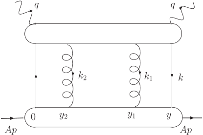
Figure 1: Two-gluon interaction in DIS

In general, the leading (or nuclear enhanced) twist-four contributions at all orders in $\alpha_{\rm s}$ to the hadronic tensor of DIS off a nucleus involving a secondary scattering with another gluon (see Fig. 1) can be written as

$$W^{(2)}_{\mu\nu} = \int\frac{d^{4}k}{(2\pi)^{4}}\int\frac{d^{4}k_{1}}{(2\pi)^{4}}\int\frac{d^{4}k_{2}}{(2\pi)^{4}}\int d^{4}y\int d^{4}y_{1}\int d^{4}y_{2}\,e^{iky+ik_{1}y_{1}+ik_{2}y_{2}}$$ (2)

$$\times \frac{1}{p\cdot n}{\rm Tr}[\hat{H}^{\rho\sigma}_{\mu\nu}(k,k_{1},k_{2})\frac{p\!\!/}{2}]\langle A\mid\bar{\psi}(0)\frac{n\!\!\!/}{2}A_{\rho}(y_{1})A_{\sigma}(y_{2})\psi(y)\mid A\rangle$$

where $\hat{H}^{\rho\sigma}_{\mu\nu}(k,k_{1},k_{2})$ is the perturbative hard part of the multiple parton scattering at any order of the strong coupling constant, $n=[0,1,\vec{0}_{\perp}]$ and $\bar{n}=[1,0,\vec{0}_{\perp}]$ are unit four-vectors. Here we have suppressed the color index. Summations over color indices of the field operators in the matrix element and average over the color indices of the initial state partons in the hard part are understood. To simplify the notation, we will sometimes suppress the polarization indices associated with the photon interaction when they are not necessary, $\hat{H}^{\rho\sigma}(k,k_{1},k_{2})\equiv\hat{H}^{\rho\sigma}_{\mu\nu}(k,k_{1},k_{2})$. In the above expression, one can always assume collinear approximation for the quark fields, $k=xp$. The transverse momentum of the quark will only contribute to high twist contributions that are not nuclear enhanced. We can further neglect the minus-components of the gluon’s momentum, which also contribute to higher-twist terms that are not nuclear enhanced. One can therefore express the gluon’s 4-momentum as $k_{1}^{\rho}=x_{1}p^{\rho}+k^{\rho}_{1\bot}$, $k_{2}^{\rho}=x_{2}p^{\rho}+k^{\rho}_{2\bot}$. One can also decompose gluon fields as $A^{\rho}=A^{\rho}_{\bot}+A^{\rho}_{+}+A^{\rho}_{-}$. Here $A^{\rho}_{\bot}=A_{\sigma}d^{\rho\sigma}$, $A^{\rho}_{+}=p^{\rho}A\cdot n/p\cdot n$, $A^{\rho}_{-}=n^{\rho}A\cdot p/p\cdot n$, and $d_{\rho\sigma}=-g_{\rho\sigma}+\bar{n}_{\rho}n_{\sigma}+n_{\rho}\bar{n}_{\sigma}$ is the transverse projection ($d_{\rho\sigma}A^{\rho}B^{\sigma}=\vec{A}_{\perp}\cdot\vec{B}_{\perp}$).

2.1 Light-cone gauge

Let us first consider the above hadronic tensor in the light-cone gauge , $A^{\rho}_{+}=0$. In this case, $A^{\rho}_{-}$ component contributes only to higher twist (beyond twist-4). Therefore, the matrix elements of the non-perturbative part of the hadronic tensor only involve one term;

$$\langle A\mid\bar{\psi}(0)n\!\!\!/A_{\bot}^{\rho}(y_{1})A_{\bot}^{\sigma}(y_{2})\psi(y)\mid A\rangle$$

$$\hskip 72.26999pt=-\frac{1}{2}d^{\rho\sigma}\langle A\mid\bar{\psi}(0)n\!\!\!/\vec{A}_{\bot}(y_{1})\cdot A_{\bot}(y_{2})\psi(y)\mid A\rangle,$$ (3)

for unpolarized nuclei.

Taking collinear approximation (neglecting gluons’ transverse momentum), one can carry out all the integrations except $y_{i}^{-}$ and $k_{i}^{+}=x_{i}p^{+}$. One can further integrate by parts in $y_{1}^{-},y_{2}^{-}$ to convert $-x_{1}p^{+}\vec{A}_{\bot}(y_{1}^{-})\cdot x_{2}p^{+}\vec{A}_{\bot}(y_{2}^{-})$ into gluon field strength, $\partial_{+}\vec{A}_{\bot}(y_{1})\cdot\vec{\partial}_{+}A_{\bot}(y_{2})=\vec{F}_{+\bot}(y_{1}^{-})\cdot\vec{F}_{+\bot}(y_{2}^{-})$ (Note that $\vec{F}_{+\bot}=\partial_{+}\vec{A}_{\bot}$ in the light-cone gauge, $A^{+}=0$). The hadronic tensor in the light-cone gauge can be reduced to

$$W^{(2)} = \int\frac{dy^{-}}{2\pi}\frac{dy^{-}_{1}}{2\pi}\frac{dy^{-}_{2}}{2\pi}\int dxdx_{1}dx_{2}e^{ix_{1}p^{+}y_{1}^{-}+ix_{2}p^{+}y_{2}^{-}+ixp^{+}y^{-}}$$ (4)

$$\times \langle A\mid\bar{\psi}(0)\frac{n\!\!\!/}{2}\vec{F}_{+\bot}(y^{-}_{1})\cdot\vec{F}_{+\bot}(y^{-}_{2})\psi(y^{-})\mid A\rangle$$

$$\times {\rm Tr}[\hat{H}^{\rho\sigma}(xp,x_{1}p,x_{2}p)\frac{p\!\!/d_{\rho\sigma}}{4x_{1}x_{2}}],$$

where we have suppressed both the $+$ and transverse components of the coordinates when they are set to zero, $y^{+}=0$, $\vec{y}_{\perp}=0$, in variables of the field operators.

The above formula is normally used to calculate contributions from double hard scattering where gluons carry finite momentum fraction $x_{1}$ and $x_{2}$. However, in soft scattering processes, the momentum fractions $x_{1}$ and $x_{2}$ go to zero. One should then choose a regularization prescription on these light-cone poles corresponding to specific boundary conditions for the gluon field [16]. In principal, all the prescriptions are equivalent for the complete set of diagrams. Alternatively, one can calculate both types of multiple parton scattering and their interferences in the covariant gauge as was outlined by LQS [10].

2.2 Covariant gauge

In the covariant gauge, both the transverse and plus components of the gluon fields contribute to the same twist operators while the minus component contributes only to higher twist terms. The matrix elements of the non-perturbative part can therefore be expanded into four terms,

$$\langle A\mid\bar{\psi}(0)[A_{+}^{\rho}(y_{1}^{-})A_{+}^{\sigma}(y^{-}_{2}) + A_{+}^{\rho}(y_{1}^{-})A_{\bot}^{\sigma}(y_{2}^{-})+A_{\bot}^{\rho}(y_{1}^{-})A_{+}^{\sigma}(y_{2}^{-})$$

$$+ A_{\bot}^{\rho}(y_{1}^{-})A_{\bot}^{\sigma}(y_{2}^{-})]\psi(y^{-})\mid A\rangle.$$

To isolate the leading terms of the twist-4 contribution with nuclear enhancement, one can follow LQS [10] to make the following collinear expansion of the perturbative hard part in terms of the gluon transverse momentum  ,

$$\hat{H}^{\rho\sigma}(k,k_{1},k_{2}) = \hat{H}^{\rho\sigma}(k,x_{1}p,x_{2}p)+\frac{\partial\hat{H}^{\rho\sigma}(k,k_{1},x_{2}p)}{\partial k_{1}^{\alpha}}\mid_{k_{1}=x_{1}p}k_{1\bot}^{\alpha}$$

$$+ \frac{\partial\hat{H}^{\rho\sigma}(k,x_{1}p,k_{2})}{\partial k_{2}^{\alpha}}\mid_{k_{2}=x_{2}p}k_{2\bot}^{\alpha}$$

$$+ \frac{\partial^{2}\hat{H}^{\rho\sigma}(k,k_{1},k_{2})}{\partial k_{1}^{\alpha}\partial k_{2}^{\beta}}\mid_{k_{1}=x_{1}p,k_{2}=x_{2}p}k_{1\bot}^{\alpha}k_{2\bot}^{\beta}+...$$

where terms $\partial^{2}\hat{H}^{\rho\sigma}/\partial k_{1}^{\alpha}\partial k_{1}^{\beta}$ and $\partial^{2}\hat{H}^{\rho\sigma}/\partial k_{2}^{\alpha}\partial k_{2}^{\beta}$ are not listed as they don’t contribute to the nuclear enhanced twist-4 terms. The first (collinear) term can be reduced to the eikonal term of the twist-2 contribution making the twist-2 quark distribution function gauge invariant. The rest of the expansion will contribute to higher twist terms. Again, after integration by parts and considering $\partial_{+}A_{\bot}^{\rho}\partial_{+}A_{\bot}^{\sigma}=\partial_{+}\vec{A}_{\bot}\cdot\partial_{+}\vec{A}_{\bot}d^{\rho\sigma}/2$, $\partial_{+}A_{\bot}^{\rho}\partial_{\bot}^{\sigma}A_{+}=\partial_{+}\vec{A}_{\bot}\cdot\vec{\partial}_{\bot}A_{+}d^{\rho\sigma}/2$, $\partial_{\bot}^{\rho}A_{+}\partial_{\bot}^{\sigma}A_{+}=\vec{\partial}_{\bot}A_{+}\cdot\vec{\partial}_{\bot}A_{+}d^{\rho\sigma}/2$ in a unpolarized nuclear target, one gets

$$W^{(2)} = \frac{1}{8}\int\frac{dy^{-}}{2\pi}\frac{dy^{-}_{1}}{2\pi}\frac{dy^{-}_{2}}{2\pi}\int dx_{1}dx_{2}dxe^{ix_{1}p^{+}y_{1}^{-}+ix_{2}p^{+}y_{2}^{-}+ixp^{+}y^{-}}$$ (6)

$$\left\{d^{\alpha\beta}{\rm Tr}\left[\frac{\partial^{2}\hat{H}_{\rho\sigma}(k,k_{1},k_{2})}{\partial k_{1}^{\alpha}\partial k_{2}^{\beta}}p\!\!/p^{\rho}p^{\sigma}\right]_{k_{1}=x_{1}p,k_{2}=x_{2}p}\right.$$

$$\hskip 36.135pt\times\langle A\mid\bar{\psi}(0)n\!\!\!/\vec{\partial}_{\bot}A_{+}(y_{1}^{-})\cdot\vec{\partial}_{\bot}A_{+}(y^{-}_{2})\psi(y^{-})\mid A\rangle$$

$$+ d^{\alpha\sigma}{\rm Tr}\left[\frac{\partial\hat{H}_{\rho\sigma}(k,x_{1}p,k_{2})}{\partial k_{2}^{\alpha}}\frac{p\!\!/p^{\rho}}{x_{1}}\right]_{k_{2}=x_{2}p}$$

$$\hskip 36.135pt\times\langle A\mid\bar{\psi}(0)n\!\!\!/\partial_{+}\vec{A}_{\bot}(y_{1}^{-})\cdot\vec{\partial}_{\bot}A_{+}(y^{-}_{2})\psi(y^{-})\mid A\rangle$$

$$+ d^{\alpha\rho}{\rm Tr}\left[\frac{\partial\hat{H}_{\rho\sigma}(k,k_{1},x_{2}p)}{\partial k_{1}^{\alpha}}\frac{p\!\!/p^{\sigma}}{x_{2}}\right]_{k_{1}=x_{1}p}$$

$$\hskip 36.135pt\times\langle A\mid\bar{\psi}(0)n\!\!\!/\vec{\partial}_{\bot}A_{+}(y^{-}_{1})\cdot\partial_{+}\vec{A}_{\bot}(y_{2}^{-})\psi(y^{-})\mid A\rangle$$

$$+ d^{\rho\sigma}{\rm Tr}\left[\hat{H}_{\rho\sigma}(k,x_{1}p,x_{2}p)\frac{p\!\!/}{x_{1}x_{2}}\right]$$

$$\hskip 36.135pt\times\langle A\mid\bar{\psi}(0)n\!\!\!/\partial_{+}\vec{A}_{\bot}(y^{-}_{1})\cdot\partial_{+}\vec{A}_{\bot}(y_{2}^{-})\psi(y^{-})\mid A\rangle\ \}.$$

Using the following identities which we will prove in the next section,

$$d^{\alpha\beta}\frac{\partial^{2}}{\partial k_{1}^{\alpha}\partial k_{2}^{\beta}}\left.\hat{H}_{\rho\sigma}(k,k_{1},k_{2})p^{\rho}p^{\sigma}\right|_{k_{1}=x_{1}p,k_{2}=x_{2}p}$$

$$\hskip 86.72377pt=d^{\rho\sigma}\hat{H}_{\rho\sigma}(k,x_{1}p,x_{2}p)\frac{1}{x_{1}x_{2}}$$

$$\hskip 86.72377pt=-d^{\alpha\sigma}\frac{\partial}{\partial k_{2}^{\alpha}}\hat{H}_{\rho\sigma}(k,x_{1}p,k_{2})\mid_{k_{2}=x_{2}p}p^{\rho}\frac{1}{x_{1}}$$

$$\hskip 86.72377pt=-d^{\alpha\rho}\frac{\partial}{\partial k_{1}^{\alpha}}\hat{H}_{\rho\sigma}(k,k_{1},x_{2}p)\mid_{k_{1}=x_{1}p}p^{\sigma}\frac{1}{x_{2}}$$ (7)

one can reorganize the hadronic tensor in the covariant gauge as

$$W^{(2)} = \frac{1}{8}\int\frac{dy^{-}}{2\pi}\frac{dy^{-}_{1}}{2\pi}\frac{dy^{-}_{2}}{2\pi}\int dx_{1}dx_{2}dxe^{ix_{1}p^{+}y_{1}^{-}+ix_{2}p^{+}y_{2}^{-}+ixp^{+}y^{-}}$$ (8)

$$\times d^{\alpha\beta}{\rm Tr}\left[\frac{\partial^{2}\hat{H}^{\rho\sigma}(k,k_{1},k_{2})}{\partial k_{1}^{\alpha}\partial k_{2}^{\beta}}p\!\!/p_{\rho}p_{\sigma}\right]_{k_{1}=x_{1}p,k_{2}=x_{2}p}\langle A\mid\bar{\psi}(0)n\!\!\!/$$

$$\times \left\{\vec{\partial}_{\bot}A_{+}(y_{1}^{-})\cdot\vec{\partial}_{\bot}A_{+}(y^{-}_{2})-\partial_{+}\vec{A}_{\bot}(y_{1}^{-})\cdot\vec{\partial}_{\bot}A_{+}(y^{-}_{2})\right.$$

$$\left.-\vec{\partial}_{\bot}A_{+}(y^{-}_{1})\cdot\partial_{+}\vec{A}_{\bot}(y_{2}^{-})+\partial_{+}\vec{A}_{\bot}(y^{-}_{1})\cdot\partial_{+}\vec{A}_{\bot}(y_{2}^{-})\right\}\psi(y^{-})\mid A\rangle$$

$$= \int\frac{dy^{-}}{2\pi}\frac{dy^{-}_{1}}{2\pi}\frac{dy^{-}_{2}}{2\pi}\int dx_{1}dx_{2}dxe^{ix_{1}p^{+}y_{1}^{-}+ix_{2}p^{+}y_{2}^{-}+ixp^{+}y^{-}}$$

$$\frac{d^{\alpha\beta}}{4}{\rm Tr}\left[\frac{\partial^{2}\hat{H}^{\rho\sigma}(k,k_{1},k_{2})}{\partial k_{1}^{\alpha}\partial k_{2}^{\beta}}p\!\!/p_{\rho}p_{\sigma}\right]_{k_{1}=x_{1}p,k_{2}=x_{2}p}$$

$$\hskip 72.26999pt\times\langle A\mid\bar{\psi}(0)\frac{n\!\!\!/}{2}\vec{F}_{+\bot}(y^{-}_{1})\cdot\vec{F}_{+\bot}(y^{-}_{2})\psi(y^{-})\mid A\rangle\,,$$

where we have neglected higher order corrections to the definition of the gluon field strength $F_{+\bot}$ in the covariant gauge. In the original derivation of the twist expanion framework [10], LQS neglected terms that are proportional to the transverse gluon fields in the covariant gauge in Eq. (6), arguing that these contributions are suppressed by $1/p^{+}$. As we have shown in the above, the corresponding hard partonic parts of all these contributions are equivalent, allowing us to combine all terms. The final result is proportional to the correlation of total field strength with one common hard partonic parts. Since the gluon field strength correlator is now in a gauge invariant form (with gauge links from other soft gluon interaction), the hard partonic parts should also be gauge invariant and can be calculated in any gauge.

Comparing Eqs. (4) and (8), the leading nuclear enhanced twist-4 contributions to the hadronic tensor of DIS off a large nucleus in both light-cone and covariant gauge have the same non-perturbative matrix elements for two-parton correlation functions. Since these matrix elements are gauge invariant, the corresponding hard parts should be equivalent and also gauge invariant, therefore can be calculated in any given gauge. The equivalence of the corresponding hard parts can be proved in all orders as given by the identity in Eq. (7).

3 Equivalence of hard parts

In this section we will prove the identities in Eq. (7). The technique of Ward identity has been used frequently in the proof of factorization in pQCD hard processes in which longitudinal gluons can be factorized from the hard part and give rise to eikonal lines in hard scattering [17]. This method is also the basic ingredient in our proof of the identities that are used to prove the equivalence of the hard parts in the leading twist-4 contributions to DIS off a large nucleus in the light-cone and covariant gauge.

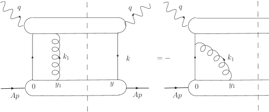
Figure 2: Diagrammtic Ward identity(dash line represent the cut)

We first consider a right-cut diagram with a single external gluon attached to the hard part in Fig. 2. The gluon momentum is ${k^{\rho}_{1}}=x_{1}p^{\rho}+k^{\rho}_{1\bot}$. We again neglect the minus component of the gluon momentum which only contributes to higher twist terms. Assuming the total amplitude $\hat{\cal M}^{\rho}$ that includes all possible gluon attachment to the hard part, gauge invariance, $\hat{\cal M}_{\rho}k_{1}^{\rho}=0$, leads to the following Ward identity,

$$\hat{H_{\rho}}(k,k_{1})k_{1}^{\rho}u(k-k_{1})=-\hat{H}(k)\frac{i}{k\!\!\!/}ik\!\!\!/_{1}u(k-k_{1}),$$ (9)

as shown diagrammatically in Fig. 2, where $u(k)$ is the quark spinor, $\hat{H_{\rho}}(k,k_{1})$ represents the hard part with one gluon attached after the photon coupling and $\hat{H}(k)$ represents the hard part without any gluon attachment. Using equation of motion $(k\!\!\!/-k\!\!\!/_{1})u(k-k_{1})=0$, we get,

$$\hat{H_{\rho}}(k,k_{1})k_{1}^{\rho}u(k-k_{1})=\hat{H}(k)u(k-k_{1})$$ (10)

Truncating the quark spinor which sits inside the non-perturbative parton matrix elements, we have the following general identity which is also valid for the diagram with the off-shell initial-state quarks,

$$\hat{H_{\rho}}(k,k_{1})k_{1}^{\rho}=\hat{H}(k)$$ (11)

Making a collinear expansion in $k_{1}^{\rho}=x_{1}p^{\rho}+k^{\rho}_{1\bot}$ of the left side,

$$\hat{H_{\rho}}(k,k_{1})k_{1}^{\rho}=\hat{H_{\rho}}(k,x_{1}p)x_{1}p^{\rho} + \hat{H_{\rho}}(k,x_{1}p)k_{1\bot}^{\rho}$$ (12)

$$+ \left.\frac{\partial{\hat{H_{\rho}}(k,k_{1})}}{\partial{k_{1}^{\alpha}}}\right|_{k_{1}=x_{1}p}k_{1\bot}^{\alpha}x_{1}p^{\rho}+....$$

and using Eq. (11) for both $k_{1}$ and $x_{1}p$, $\hat{H_{\rho}}(k,x_{1}p)x_{1}p^{\rho}=\hat{H}(k)=\hat{H_{\rho}}(k,k_{1})k_{1}^{\rho}$, we obtain the following identity,

$$\left.\frac{\partial{\hat{H_{\rho}}(k,k_{1})}}{\partial{k_{1}^{\alpha}}}\right|_{k_{1}=x_{1}p}k_{1\bot}^{\alpha}x_{1}p^{\rho}=-\hat{H_{\rho}}(k,x_{1}p)k^{\rho}_{1\bot}$$ (13)

Note that authors of the Ref [18] have recently derived the above identity case by case.

For diagrams with two attached gluons that contribute to twist-4 terms, one can derive two identities similar to Eq. (11) by contracting with the momentum of gluon 1 and gluon 2, $k_{1}$, $k_{2}$ and then make collinear expansion in them respectively,

$$\left.\frac{\partial{\hat{H}_{\rho\sigma}(k,k_{1},k_{2})}}{\partial{k_{1}^{\alpha}}}\right|_{k_{1}=x_{1}p}\!\!\!\!k_{1\bot}^{\alpha}x_{1}p^{\rho} = -\hat{H}_{\rho\sigma}(k,x_{1}p,k_{2})k^{\rho}_{1\bot}$$ (14)

$$\left.\frac{\partial{\hat{H}_{\rho\sigma}(k,k_{1},k_{2})}}{\partial{k_{2}^{\beta}}}\right|_{k_{2}=x_{2}p}\!\!\!\!k_{2\bot}^{\beta}x_{2}p^{\sigma} = -\hat{H}_{\rho\sigma}(k,k_{1},x_{2}p)k^{\sigma}_{2\bot}$$ (15)

Making again collinear expansion in $k_{2\bot}$ on both sides of Eq. (14), multiplying both sides with $x_{2}p^{\sigma}$ and using Eq. (15) with $k_{1}=x_{1}p$, one has

$$\left.\frac{\partial^{2}{\hat{H}_{\rho\sigma}(k,k_{1},k_{2})}}{\partial{k_{1}^{\alpha}}\partial{k_{2}^{\beta}}}\right|_{k_{1}=x_{1}p,k_{2}=x_{2}p} k_{1\bot}^{\alpha}k_{2\bot}^{\beta}x_{1}p^{\rho}x_{2}p^{\sigma}$$ (16)

$$=\left.-\frac{\partial\hat{H}_{\rho\sigma}(k,x_{1}p,k_{2})}{\partial k_{2}^{\beta}}\right|_{k_{2}=x_{2}p}\!\!\!\!k_{2\bot}^{\beta}k^{\rho}_{1\bot}x_{2}p^{\sigma}$$

$$=\hat{H}_{\rho\sigma}(k,x_{1}p,x_{2}p)k_{1\bot}^{\rho}k^{\sigma}_{2\bot}$$

Similarly making collinear expansion in $k_{1\bot}$ on both sides of Eq. (15), multiplying both sides with $x_{1}p^{\rho}$ and using Eq. (14) with $k_{2}=x_{2}p$ gives,

$$\left.\frac{\partial^{2}{\hat{H}_{\rho\sigma}(k,k_{1},k_{2})}}{\partial{k_{1}^{\alpha}}\partial{k_{2}^{\beta}}}\right|_{k_{1}=x_{1}p,k_{2}=x_{2}p} k_{1\bot}^{\alpha}k_{2\bot}^{\beta}x_{1}p^{\rho}x_{2}p^{\sigma}$$ (17)

$$=\left.-\frac{\partial\hat{H}_{\rho\sigma}(k,x_{1}p,k_{2})}{\partial k_{1}^{\alpha}}\right|_{k_{1}=x_{1}p}\!\!\!\!k_{1\bot}^{\alpha}k^{\sigma}_{2\bot}x_{1}p^{\rho}$$

$$=\hat{H}_{\rho\sigma}(k,x_{1}p,x_{2}p)k_{1\bot}^{\rho}k^{\sigma}_{2\bot}$$

We can further integrate the above two sets of equations over the azimuthal angle of the gluons’ transverse momentum, divide both sides by $x_{1}x_{2}$ and obtain finally the identities in Eqs.(7),

$$d^{\alpha\beta}\left.\frac{\partial^{2}\hat{H}^{\rho\sigma}(k,k_{1},k_{2})}{\partial k_{1}^{\alpha}\partial k_{2}^{\beta}}p_{\rho}p_{\sigma}\right|_{k_{1}=x_{1}p,k_{2}=x_{2}p} =d^{\rho\sigma}\hat{H}^{\rho\sigma}(k,x_{1}p,x_{2}p)\frac{1}{x_{1}x_{2}}$$ (20)

$$=-d^{\alpha\sigma}\left.\frac{\partial\hat{H}^{\rho\sigma}(k,x_{1}p,k_{2})}{\partial k_{2}^{\alpha}}\frac{p_{\rho}}{x_{1}}\right|_{k_{2}=x_{2}p}$$

$$=-d^{\alpha\rho}\left.\frac{\partial\hat{H}^{\rho\sigma}(k,k_{1},x_{2}p)}{\partial k_{1}^{\alpha}}\frac{p_{\sigma}}{x_{2}}\right|_{k_{1}=x_{1}p}\,.$$

4 DIS in leading order

The general proof of the identities for the hard parts in the previous section is valid for all orders in $\alpha_{\rm s}$. In this and next section, we will calculate nuclear modification to the semi-inclusive cross section of DIS off a large nucleus up to $\cal{O}$$(\alpha_{s})$ as an explicit example to demonstrate the gauge invariance.

Figure 3: DIS in lowest order with zero, one and two gluon exchange between the final quark and the target remnant

The semi-inclusive cross section off DIS in Eq. (1) at the lowest order in $\alpha_{s}$ has been calculated in Ref. [19] up to two gluon exchanges as shown in Fig. 3. The semi-inclusive hadronic tensor can be expanded in terms of the number of physical gluon exchanges [19] $W_{\mu\nu}(q,p,\ell)=\sum_{i}W_{\mu\nu}^{(i)}(q,p,\ell)$,

$$\frac{d^{2}W_{\mu\nu}^{(0)}}{d^{2}\ell_{\perp}} = \frac{1}{2\pi}\int\frac{d^{4}k}{(2\pi)^{4}}\delta^{(2)}(\vec{\ell}_{\perp}-\vec{k}_{\perp}){\rm Tr}[\hat{H}_{\mu\nu}^{(0)}(x)\ \hat{\Phi}^{(0)}(k)];$$ (21)

$$\frac{d^{2}W_{\mu\nu}^{(1)}}{d^{2}\ell_{\perp}} = \frac{1}{2\pi}\int\frac{d^{4}k}{(2\pi)^{4}}\frac{d^{4}k_{1}}{(2\pi)^{4}}\sum_{c=L,R}\delta^{(2)}(\vec{\ell}_{\perp}-\vec{k}_{c\perp})$$ (22)

$$\times{\rm Tr}[\hat{H}_{\mu\nu}^{(1,c)\rho}(x,x_{1})\omega_{\rho}^{\ \rho^{\prime}}\hat{\Phi}^{(1)}_{\rho^{\prime}}(k_{1},k)];$$

$$\frac{d^{2}W_{\mu\nu}^{(2)}}{d^{2}\ell_{\perp}} = \frac{1}{2\pi}\int\frac{d^{4}k_{1}}{(2\pi)^{4}}\frac{d^{4}k_{2}}{(2\pi)^{4}}\frac{d^{4}k}{(2\pi)^{4}}\sum_{c=L,R,C}\delta^{(2)}(\vec{\ell}_{\perp}-\vec{k}_{c\perp})$$ (23)

$$\times{\rm Tr}[\hat{H}_{\mu\nu}^{(2,c)\rho\sigma}(x,x_{1},x_{2})\omega_{\rho}^{\ \rho^{\prime}}\omega_{\sigma}^{\ \sigma^{\prime}}\hat{\Phi}^{(2)}_{\rho^{\prime}\sigma^{\prime}}(k_{1},k_{2},k)],$$

where the summation is over different cut diagrams with given number of gluon exchanges, $\hat{H}_{\mu\nu}^{(0)}$, $\hat{H}_{\mu\nu}^{(1,c)\rho}$ and $\hat{H}_{\mu\nu}^{(2,c)\rho\sigma}$ are the hard parts of the corresponding cut diagrams (see Ref. [19] for details). For single gluon exchange, $\vec{k}_{R\perp}=\vec{k}_{\perp}$, $\vec{k}_{L\perp}=\vec{k}_{\perp}+\vec{k}_{1\perp}$ For two gluon exchange diagram, $\vec{k}_{R\perp}=\vec{k}_{\perp}$, $\vec{k}_{C\perp}=\vec{k}_{\perp}+\vec{k}_{1\perp}$ and $\vec{k}_{L\perp}=\vec{k}_{\perp}+\vec{k}_{1\perp}+\vec{k}_{2\perp}$. The projection operator is defined such that $\omega_{\rho}^{\sigma}k_{i\sigma}=(k_{i}-x_{i}p)_{\rho}$. The above expression for semi-inclusive cross section is obtained through collinear expansion in $(k_{i}-x_{i}p)$ of the partonic hard parts and the decomposition of the gauge field $A_{\rho}=p_{\rho}A^{+}/p^{+}+\omega_{\rho}^{\sigma}A_{\sigma}$. Generalized Ward identities are used to relate the derivatives of the partonic hard parts to the hard parts with extra longitudinal gluon attachments. Consequently, the unintegrated parton matrix elements contain contributions from all Feynman diagrams with different number of unphysical gluon exchanges between the propagating quark and the nucleus. They can be defined in a gauge invariant way as,

$$\hat{\Phi}^{(0)}(k) = \int d^{4}ye^{ik\cdot y}\langle A|\bar{\psi}(0){\cal L}(0,y)\psi(y)|A\rangle,$$ (24)

$$\hat{\Phi}^{(1)}_{\rho}(k_{1},k) = \int d^{4}yd^{4}y_{1}e^{ik\cdot y+ik_{1}\cdot y_{1}}\langle A|\bar{\psi}(0){\cal L}(0,y_{1})D_{\rho}(y_{1}){\cal L}(y_{1},y)\psi(y)|A\rangle,$$

$$\hat{\Phi}^{(2)}_{\rho\sigma}(k_{1},k_{2},k) = \int d^{4}yd^{4}y_{1}d^{4}y_{2}e^{ik\cdot y+ik_{1}\cdot y_{1}+ik_{2}\cdot y_{2}}$$

$$\times \langle A|\bar{\psi}(0){\cal L}(0,y_{2})D_{\rho}(y_{2}){\cal L}(y_{2},y_{1})D_{\sigma}(y_{1}){\cal L}(y_{1},y)\psi(y)|A\rangle,$$

where $D_{\rho}(y)=\partial_{\rho}+igA_{\rho}(y)$ is the covariant derivative and

$${\cal L}(y_{2},y_{1}) \equiv {\cal L}^{\dagger}_{\parallel}(-\infty,y_{2}^{-};\vec{y}_{2\perp}){\cal L}^{\dagger}_{\perp}(-\infty;\vec{y}_{2\perp},\vec{y}_{1\perp}){\cal L}_{\parallel}(-\infty,y^{-}_{1};\vec{y}_{1\perp})$$ (27)

is the complete gauge link that contains both the transverse [20]

$${\cal L}_{\perp}(-\infty;\vec{y}_{2\perp},\vec{y}_{1\perp})\equiv P\exp\left[-ig\int_{\vec{y}_{2\perp}}^{\vec{y}_{1\perp}}d\vec{\xi}_{\perp}\cdot\vec{A}_{\perp}(-\infty,\vec{\xi}_{\perp})\right]$$ (28)

and longitudinal gauge link

$${\cal L}_{\parallel}(-\infty,y^{-};\vec{y}_{\perp})\equiv P\exp\left[-ig\int^{-\infty}_{y^{-}}d\xi^{-}A_{+}(\xi^{-},\vec{y}_{\perp})\right].$$ (29)

The exchange of unphysical gluon between the propagating quark and the nucleus therefore leads to the gauge links in the parton matrix elements while physical gluons lead to the higher-twist contributions to the DIS cross section which are characterized by the covariant derivatives $D_{\rho}$ in the higher-twist parton matrix elements. The spatial derivative in $D_{\rho}$ comes from the collinear expansion of the partonic hard parts while the transverse gluon field in $D_{\rho}$ corresponds to interaction between the propagating quark and a physical gluon from the nucleus.

We refer the above organization of semi-inclusive DIS cross section within the collinear expansion as a generalized twist-expansion in which each contribution involves a parton matrix element with a given number of covariant derivatives. These parton matrix elements correspond to unintegrated parton distributions. Note that after integration (over both $k^{-}$ and $\vec{k}_{\perp}$), each of these unintegrated parton distributions will give rise to a mixture of collinear (or integrated) parton distributions or parton matrix elements with different dimensions, because of the off-shellness and transverse momentum carried by each parton.

The nuclear enhanced twist-four contributions to the semi-inclusive cross section at the leading order is contained in Eq. (23) with the corresponding projected parton matrix elements $\omega_{\rho}^{\rho^{\prime}}\omega_{\sigma}^{\sigma^{\prime}}\hat{\Phi}^{(2)}_{\rho^{\prime}\sigma^{\prime}}(k_{1},k_{2},k)$ in Eq. (4) which is apparently gauge invariant. Note that the leading components of the projected covariant derivative $\omega_{\rho}^{\rho^{\prime}}D_{\rho^{\prime}}$ are the transverse ones, $\vec{D}_{\perp}=\vec{\partial}_{\perp}+ig\vec{A}_{\perp}$. Using the following identity [21],

$$i\vec{\partial}_{y_{\perp}}{\cal L}(y_{1},y) = {\cal L}(y_{1},y)\left[i\vec{D}_{\perp}(y^{-},\vec{y}_{\perp})\right.$$ (30)

$$+ \left.g\int_{-\infty}^{y^{-}}d\xi^{-}{\cal L}^{\dagger}_{\parallel}(\xi^{-},y^{-};\vec{y}_{\perp})\vec{F}_{+\perp}(\xi^{-},\vec{y}_{\perp}){\cal L}_{\parallel}(\xi^{-},y^{-};\vec{y}_{\perp})\right],$$

it is easy to see that the parton matrix element $\omega_{\rho}^{\rho^{\prime}}\omega_{\sigma}^{\sigma^{\prime}}\hat{\Phi}^{(2)}_{\rho^{\prime}\sigma^{\prime}}(k_{1},k_{2},k)$ in Eq. (4) contains exactly the same quark-gluon correlation distribution in Eqs. (4) and (8). Note that the hard part in Eq. (23) is projected to the transverse polarization of the gluon exchange and therefore corresponds to interaction with collinear physical gluons in the light-cone gauge. In the derivation [19] of this final form, Ward indentities are also used to relate it to the derivative of the hard parts for quark and longitudinal gluon interaction in the covariant gauge.

After integration over the transverse momentum of the quark, one will be able to recover the nuclear enhanced twist-four contributions to the inclusive DIS cross section [22, 23], which should be power-suppressed by $1/Q^{2}$. In the calculation of the above twist-four contribution to the inclusive DIS cross section, one can similarly relate the transverse gauge field $\vec{A}_{\perp}$ to the field strength $\vec{F}_{+\perp}$ via partial integration. However, one should include the gluonic poles [16] in

$$\int dy^{-}e^{ixp^{+}y^{-}}A_{\perp}(y^{-})=\int dy^{-}e^{ixp^{+}y^{-}}\frac{1}{x\pm i\epsilon}F_{+\perp}(y^{-}),$$ (31)

depending on the boundary condition for $A_{\perp}(\pm\infty)$ which do not vanish simultaneously in the light-cone gauge [24]. We have chosen $\vec{A}_{\perp}(\infty)=0$ in this paper. Such gluonic poles have non-vanishing contributions to higher-twist inclusive cross sections of DIS which are suppressed by $1/Q^{2}$. Without inclusion of these gluonic pole contributions, one could be misled to the conclusion [25] that interaction with physical transverse gluons in the light-cone gauge could lead to leading twist transverse momentum broadening of a propagating quark, which does not contribute to higher-twist ($1/Q^{2}$ suppressed) inclusive cross section. As we will show in the next section, such transverse momentum broadening comes from interaction with unphysical gluons (either longitudinal gluon $A_{+}$ in covariant gauge or pure transverse gauge field $\vec{A}_{\perp}(-\infty)$ at the light-cone infinity in the light-cone gauge).

5 Nuclear transverse momentum broadening

Even though the exchange of unphysical gluons do not contribute to the hard parts of higher-twist DIS cross sections, they do lead to important gauge links in parton distributions and the transverse momentum broadening of the propagating quark inside a nucleus at the leading twist (no $1/Q^{2}$ suppression). Exchange of physical gluons (e.g. transverse gluons) only leads to higher-twist inclusive cross section and transverse momentum broadening which is suppressed by factors of $1/Q^{2}$ as compared to the leading twist broadening. This has been a source of confusion in previous studies.

Consider the semi-inclusive hadronic tensor with no physical gluon exchange in Eq. (21). The collinear component of the parton matrix element

$$\hat{\Phi}^{(0)}(k)=\frac{1}{2}p\!\!\!/\hat{f}_{A}^{q}(k)+\frac{1}{2}(k\!\!\!/-xp\!\!\!/)\hat{f}_{\perp A}^{q}(k)$$ (32)

will give rise to the leading twist contribution to the semi-inclusive hadronic tensor

$$\frac{d^{2}W_{\mu\nu}^{(0)}}{d^{2}\ell_{\perp}}=\frac{1}{2\pi}\int dxd^{2}k_{\perp}\delta^{(2)}(\vec{\ell}_{\perp}-\vec{k}_{\perp}){\rm Tr}[\hat{H}_{\mu\nu}^{(0)}(x)\frac{p\!\!\!/}{2}]f_{A}^{q}(x,\vec{k}_{\perp});\\$$ (33)

and the transverse momentum dependent quark distribution function

$$f^{q}_{A}(x,\vec{k}_{\perp}) = \int dk^{-}\hat{f}_{A}^{q}(k)=\int\frac{dy^{-}}{2\pi}\frac{d^{2}y_{\perp}}{(2\pi)^{2}}e^{ixp^{+}y^{-}-i\vec{k}_{\perp}\cdot\vec{y}_{\perp}}$$ (34)

$$\times \langle A\mid\bar{\psi}(0,\vec{0}_{\perp})\frac{\gamma^{+}}{2}{\cal L}(0,y)\psi(y^{-},\vec{y}_{\perp})\mid A\rangle.$$

The corresponding integrated quark distribution function is

$$f_{A}^{q}(x) = \int d^{2}k_{\perp}f_{A}^{q}(x,\vec{k}_{\perp})$$ (35)

$$= \int\frac{dy^{-}}{2\pi}e^{ixp^{+}y^{-}}\langle A\mid\bar{\psi}(0,\vec{0}_{\perp})\frac{\gamma^{+}}{2}{\cal L}_{\parallel}(0,y^{-})\psi(y^{-},\vec{0}_{\perp})\mid A\rangle.$$

One can make a Taylor expansion of the gauge link and the quark field in the transverse coordinate $\vec{y}_{\perp}$ and then complete integration over $\vec{y}_{\perp}$,

$$f^{q}_{A}(x,\vec{k}_{\perp}) = \int\frac{dy^{-}}{2\pi}e^{ixp^{+}y^{-}}\langle A\mid\bar{\psi}(0,\vec{0}_{\perp})\frac{\gamma^{+}}{2}$$ (36)

$$\hskip 36.135pt\times\left[e^{i\vec{\partial}_{y_{\perp}}\cdot\vec{\partial}_{k_{\perp}}}{\cal L}(0,y)\psi(y^{-},\vec{y}_{\perp})\right]_{y_{\perp}=0}\mid A\rangle\delta^{(2)}(\vec{k}_{\perp}).$$

Using the identity in Eq. (30), one can express the above transverse momentum dependent quark distribution in terms of collinear higher-twist quark and gluon correlation matrix elements [21].

For the purpose of discussion in this paper, we consider first the quadratic term in the expansion of the gauge link in the covariant gauge,

$${\cal L}^{(2)}(0,y) = \int dy^{-}_{1}dy^{-}_{2}\left[-g^{2}A_{+}(y^{-}_{2},\vec{y}_{\perp})A_{+}(y^{-}_{1},\vec{y}_{\perp})\theta(y^{-}-y_{2}^{-})\theta(y^{-}_{2}-y_{1}^{-})\right.$$ (37)

$$+ g^{2}A_{+}(y^{-}_{2},\vec{0}_{\perp})A_{+}(y^{-}_{1},\vec{y}_{\perp})\theta(-y_{2}^{-})\theta(y^{-}-y_{1}^{-})$$

$$- \left.g^{2}A_{+}(y^{-}_{2},\vec{0}_{\perp})A_{+}(y^{-}_{1},\vec{0}_{\perp})\theta(-y_{1}^{-})\theta(y^{-}_{1}-y_{2}^{-})\right].$$

The three terms in the above expansion correspond to the left, central and right cut diagrams in Fig. 3(c). One can further expand the derivative operator $\exp(i\vec{\partial}_{y_{\perp}}\cdot\vec{\partial}_{k_{\perp}})$ to the quadratic term. It is easy to note that only the left-cut contribution has a term $F_{+\perp}(y_{2}^{-})F_{+\perp}(y^{-}_{1})\approx\partial_{\perp}A_{+}(y_{2}^{-},0_{\perp})\partial_{\perp}A_{+}(y_{1}^{-},0_{\perp})$ from the quadratic derivative $(\vec{\partial}_{y_{\perp}}\cdot\vec{\partial}_{k_{\perp}})^{2}$. As we will explain later this is the leading term that has a nuclear enhancement.

One can also express the above contributions explicitly in terms of the transverse momentum of each gluonic field as denoted in Fig. 3(c),

$${\cal L}^{(2)}(0,y)\ =\int d^{2}k_{1\perp}d^{2}k_{2\perp}\int\frac{d^{2}y_{1\perp}}{(2\pi)^{2}}\frac{d^{2}y_{2\perp}}{(2\pi)^{2}}e^{-i\vec{k}_{1\perp}\cdot\vec{y}_{1\perp}-i\vec{k}_{2\perp}\cdot\vec{y}_{2\perp}}$$

$$\hskip 36.135pt\times D(\vec{k}_{1\perp},\vec{k}_{2\perp},\vec{k}_{\perp},\vec{\ell}_{\perp})A_{+}(y^{-}_{2},\vec{y}_{2\perp})A_{+}(y^{-}_{1},\vec{y}_{1\perp})$$

$$D\equiv\int dy^{-}_{1}dy^{-}_{2}\left[-g^{2}\theta(y^{-}-y_{2}^{-})\theta(y^{-}_{2}-y_{1}^{-})\delta^{(2)}(\vec{\ell}_{\perp}-\vec{k}_{\perp}-\vec{k}_{1\perp}-\vec{k}_{2\perp})\right.$$

$$\hskip 36.135pt+g^{2}\theta(-y_{2}^{-})\theta(y^{-}-y_{1}^{-})\delta^{(2)}(\vec{\ell}_{\perp}-\vec{k}_{\perp}-\vec{k}_{1\perp})$$

$$\hskip 36.135pt\left.-g^{2}\theta(-y_{1}^{-})\theta(y^{-}_{1}-y_{2}^{-})\delta^{(2)}(\vec{\ell}_{\perp}-\vec{k}_{\perp})\right].$$ (38)

One can expand the above $\delta$-functions in the transverse momenta of the quark and gluon fields $\vec{k}_{\perp}$, $\vec{k}_{1\perp}$ and $\vec{k}_{2\perp}$. Contribution to $\partial_{\perp}A_{+}(y_{2}^{-},0_{\perp})\partial_{\perp}A_{+}(y_{1}^{-},0_{\perp})$ again comes only from the first term which corresponds to the left-cut diagram in Fig. 3(c). Since the dependence of the partonic hard part $D$ on the transverse momentum of the quark field only leads to the higher-twist matrix elements that are not nuclear enhanced, one can set $k_{\perp}=0$ in the hard part. By momentum conservation $\vec{k}_{1\perp}=-\vec{k}_{2\perp}$. In this case, only the second term from the central-cut diagram contribute to the parton matrix $\partial_{\perp}A_{+}(y_{2}^{-},0_{\perp})\partial_{\perp}A_{+}(y_{1}^{-},0_{\perp})$ for the leading nuclear broadening.

One can make a similar analysis of the transverse momentum distribution in the light-cone gauge. The leading twist contribution comes from the transverse gauge link which is determined by the boundary condition of the transverse gauge field $A_{\perp}(-\infty,\vec{y}_{\perp})$ [21]. As we have discussed before, quark interaction with physical transverse gauge field will lead to higher-twist inclusive cross section and the transverse momentum broadening which is power suppressed by $1/Q^{2}$ as compared to the leading twist contribution.

Taking the quadratic derivatives of the two-gluon contribution [Fig. 3(c)] to the gauge link in Eq. (36), one can obtain the corresponding transverse momentum distribution,

$$f_{A}^{q}(x,\vec{\ell}_{\perp}) \approx f_{A}^{q}(x)\delta^{(2)}(\vec{\ell}_{\perp})+\frac{2\pi\alpha_{s}}{N_{c}}T_{qg}^{A}(x,0)\frac{1}{4}\nabla^{2}_{\ell_{\perp}}\delta^{(2)}(\vec{\ell}_{\perp})\,,$$ (39)

where

$$T^{A}_{qg}(x,x_{1}) = \int\frac{dy^{-}}{2\pi}dy^{-}_{1}dy^{-}_{2}e^{ixp^{+}y^{-}+ix_{1}p^{+}(y_{1}^{-}-y_{2}^{-})}\theta(-y_{2}^{-})\theta(y^{-}-y_{1}^{-})$$ (40)

$$\frac{1}{2}\langle A\mid\bar{\psi}(0)\gamma^{+}\vec{F}_{+\perp}(y^{-}_{2})\cdot\vec{F}_{+\perp}(y^{-}_{1})\psi(y^{-})\mid A\rangle,$$

is the quark-gluon correlation function inside the nucleus.

The quark-gluon correlation function inside a nucleus in Eq. (40) has two types of contributions. Because a nucleus consists of nucleons which are color singlet states, the quark-gluon pair could either come from a single nucleon or from two separate nucleons. In the first case, all four parton fields in the above correlation matrix element are confined to the size of a nucleon $y^{-},y_{1}^{-},y_{2}^{-}\sim r_{N}$. On the other hand, if quark and gluon fields are confined to two separate nucleons, $y^{-},|y_{1}^{-}-y_{2}^{-}|\sim r_{N}$, the overall position of the gluon field will follow the second nucleon and are only confined to the size of the nucleus $R_{A}$. Therefore, the quark-gluon correlation function in this case will have a nuclear enhancement of the order $R_{A}/r_{N}\sim A^{1/3}$ as compared to the first case where both quark and gluon fields are confined to a single nucleon. For multiple scattering in a large nucleus, we will only keep the second correlation with nuclear enhancement. If we further neglect the correlation between different nucleons and assume the large nucleus as a weakly bound and homogenous system of nucleons, the leading contribution to the quark-gluon correlation function can be approximated as [9, 26]

$$T_{qg}^{A}(x,x_{1}) \approx f^{q}_{A}(x)\int d\xi^{-}_{N}\int\frac{d^{3}p_{N}}{(2\pi)^{3}2p^{+}_{N}}f_{A}(p_{N},\xi_{N})d\xi^{-}e^{ix_{1}p^{+}\xi^{-}}$$ (41)

$$\times \langle N\mid\vec{F}_{+\perp}(0)\cdot\vec{F}_{+\perp}(\xi^{-})\mid N\rangle$$

$$= \pi f^{q}_{A}(x)\int d\xi^{-}_{N}\rho^{A}_{N}(\xi_{N})x_{1}f^{g}_{N}(x_{1}),$$

where $p_{N}^{+}=p^{+}$ is the longitudinal momentum per nucleon and

$$xf^{g}_{N}(x)=\int\frac{d\xi^{-}}{2\pi p^{+}}e^{ixp^{+}\xi^{-}}\langle N\mid\vec{F}_{+\perp}(0)\cdot\vec{F}_{+\perp}(\xi^{-})\mid N\rangle,$$ (42)

is the gluon distribution function in a nucleon, respectively. The spatial nucleon density inside the nucleus is

$$\rho^{A}_{N}(\xi_{N})=\int\frac{d^{3}p_{N}}{(2\pi)^{3}}f_{A}(p_{N},\xi_{N}).$$

The integration over the spatial position of the nucleon $\xi^{-}_{N}=(y_{1}^{-}+y_{2}^{-})/2$ is limited to the size of the nucleus. The relative coordinate of the two gluon fields is $\xi^{-}=y_{1}^{-}-y_{2}^{-}$.

With the above approximation, the transverse momentum broadening squared of the propagating quark can be calculated as

$$\langle\Delta\ell_{\perp}^{2}\rangle\equiv\frac{1}{f_{A}^{q}(x)}\int d^{2}\ell_{\perp}\ell_{\perp}^{2}f_{A}^{q}(x,\vec{\ell}_{\perp})=\int d\xi^{-}_{N}\hat{q}_{F}(\xi_{N}),$$ (43)

where the quark transport parameter

$$q_{F}(\xi_{N})\equiv\frac{2\pi^{2}\alpha_{s}}{N_{c}}\rho^{A}_{N}(\xi_{N})[xf_{g}^{N}(x)]_{x\approx 0}$$ (44)

can be interpreted as the broadening of the mean transverse momentum squared per unit path length. One can consider multiple gluon exchanges the transverse distribution will become a Gaussian form [21, 25, 29] with the width given by the averaged transverse momentum broadening.

In the above approximation of the twist-four quark-gluon matrix we have neglected multiple-nucleon correlation in a large nucleus. Such an approximation is not valid for small $x$ where quark-gluon and gluon-gluon fusion from different nucleons become important and can lead to modification of the quark distribution function and gluon saturation in a large nucleus [27, 28]. One can take into account such effect by using a nuclear modified quark distribution function $f_{A}^{q}(x_{B})$ and saturated gluon distribution function in the transport parameter $\hat{q}_{F}$ which could lead a non-trivial nuclear and energy dependence [26].

Note that the quark-gluon correlation function as defined in Eq. (40) and the gluon distribution function in Eq.(42) are not gauge invariant in covariant gauge. One needs to resum additional number of collinear soft gluons on both side of the cut to produce gauge links that will ensure the gauge invariance of the quark-gluon correlation and the gluon distribution function. A general and gauge invariant form of the transverse momentum broadening has been derived in Ref. [21].

6 Induced gluon radiation in light-cone gauge

As another example of the equivalence of the hard parts in double parton scattering in light-cone and covariant gauge, we consider the double hard quark-gluon scattering in next leading order which has been calculated in covariant gauge in helicity amplitude approximation in Ref. [8]. In the following we will calculate the induced gluon spectra from such quark-gluon scattering in light-cone gauge approach within helicity amplitude approximation. Under such helicity amplitude approximation, we can neglect momentum transfer to the quark, except in its propagation direction and only consider its dominant minus component. Since the initial gluon fields only have transverse components in the light-cone gauge approach, their direct interaction with the quark will produce a vertex in the form $n\!\!\!/\epsilon\!\!/\!_{\perp}n\!\!\!/=0$ in the helicity amplitude approximation. Intuitively, this is because a quark can not absorb the transversely polarized gluon due to helicity conservation if we neglect the recoil induced by the interaction. For this reason, we only need to consider the quark-gluon rescattering with triple gluon vertex in the helicity amplitude approximation as shown in Fig. 4. Inclusion of the quark recoil and other diagrams in light-cone gauge will lead to power corrections in $\ell_{\perp}^{2}$ and $1-z$.

Figure 4: Radiative correction to double hard scattering

Contribution from the next-leading order double hard quark-gluon scattering can be written as,

$$\frac{dW_{\mu\nu}^{(2)}}{dz} = \sum_{q}\int\frac{dy^{-}}{2\pi}dy^{-}_{1}dy^{-}_{2}\int dx\frac{dx_{1}}{2\pi}\frac{dx_{2}}{2\pi}e^{ixp^{+}y^{-}+ix_{1}p^{+}y_{1}^{-}-ix_{2}p^{+}y_{2}^{-}}$$ (45)

$$\times\frac{d_{\rho\sigma}}{2x_{1}x_{2}}\widetilde{H}^{\rho\sigma}_{\mu\nu}(x,x_{1},x_{2},p,q,z)\langle A\mid\bar{\psi}_{q}(0)\frac{\gamma^{+}}{2}F_{+\sigma}(y_{2}^{-})F_{+}^{\;\;\sigma}(y_{1}^{-})\psi_{q}(y^{-})\mid A\rangle\,,$$

where $x_{3}=x+x_{1}-x_{2}$ by momentum conservation and $z$ is the fractional momentum carried by the final quark $\ell_{q}^{-}=zq^{-}$. The hard partonic part in general has the form,

$$\widetilde{H}^{\rho\sigma}_{\mu\nu}(x,x_{1},x_{2},p,q,z) = \int\frac{d^{4}\ell}{(2\pi)^{4}}2\pi\delta_{+}(\ell^{2})\delta(1-z-\frac{\ell^{-}}{q^{-}})$$ (46)

$$\hskip 72.26999pt\times\frac{1}{2}{\rm Tr}[p\!\!\!/\gamma_{\mu}\hat{H}^{\rho\sigma}\gamma_{\nu}]\,.$$

For the central-cut diagram of quark-gluon rescattering in Fig. 4, $\hat{H}^{\rho\sigma}$ is given by,

$$\hat{H}^{\rho\sigma} = -e_{q}^{2}Cg^{4}\frac{xp\!\!\!/+q\!\!\!/}{(xp+q)^{2}-i\epsilon}\gamma^{\alpha}\ell\!\!\!/_{q}\gamma^{\beta}\frac{x_{3}p\!\!\!/+q\!\!\!/}{(x_{3}p+q)^{2}+i\epsilon}\frac{1}{(x_{1}p-\ell)^{2}-i\epsilon}$$ (47)

$$\times\frac{2\pi\delta_{+}(\ell_{q}^{2})}{((x+x_{1}-x_{3})p-\ell)^{2}+i\epsilon}g_{\alpha\alpha^{\prime}}g_{\beta\beta^{\prime}}g_{\lambda\gamma}\Lambda^{\beta^{\prime}\lambda\rho}\Lambda^{\gamma\alpha^{\prime}\sigma}$$

$$= -e_{q}^{2}Cg^{4}\frac{(xp\!\!\!/+q\!\!\!/)\gamma^{\alpha}\ell\!\!\!/_{q}\gamma^{\beta}(x_{3}p\!\!\!/+q\!\!\!/)}{(2p\cdot q)^{4}(x-x_{B}-i\epsilon)(x_{3}-x_{B}+i\epsilon)}\frac{1}{(1-z)^{2}}$$

$$\times\frac{2\pi\delta_{+}[2zp\cdot q(x+x_{1}-x_{B}-x_{L})]}{(x_{1}+i\epsilon)(x+x_{1}-x_{3}-i\epsilon)}g_{\alpha\alpha^{\prime}}g_{\beta\beta^{\prime}}g_{\lambda\gamma}\Lambda^{\beta^{\prime}\lambda\rho}\Lambda^{\gamma\alpha^{\prime}\sigma}\,,$$

where $C=C_{A}/2N_{c}$ is the color factor, $\ell$ and $\ell_{q}=(x_{1}+x_{2})p+q-\ell$ are the momenta of the final state gluon and quark, respectively, and

$$x_{L}=\frac{\ell_{\bot}^{2}}{2p^{+}q^{-}z(1-z)}$$ (48)

is the fractional momentum taken away from the initial state quarks and gluons by the final state quark-gluon splitting. The three gluon vertices are defined as

$$\Lambda^{\beta^{\prime}\lambda\rho}=g^{\beta^{\prime}\lambda}(2\ell-x_{1}p)^{\rho}-g^{\lambda\rho}(\ell+x_{1}p)^{\beta^{\prime}}+g^{\rho\beta^{\prime}}(2x_{1}p-\ell)^{\lambda}$$

$$\Lambda^{\alpha^{\prime}\sigma\gamma}=g^{\alpha^{\prime}\sigma}(2x_{2}p-\ell)^{\gamma}-g^{\sigma\gamma}(\ell+x_{2}p)^{\alpha^{\prime}}+g^{\gamma\alpha^{\prime}}(2\ell-x_{2}p)^{\sigma}.$$ (49)

In the above, we have used gluon propagators in the Feynman gauge. Since the initial gluons only have transverse components in their polarization, we can also replace the summation of the final state gluon’s polarization tensor as $\sum_{i}\epsilon^{\lambda}(i)\epsilon^{*\gamma}(i)=-g^{\lambda\gamma}$.

One can carry out the integrations over $x$ and $x_{1}$ in Eqs. (45) and (47) by contour integration. There are four possible poles in the denominator of Eq. (47) from quark and gluon propagators. Different choices for the pair of poles represent subprocesses with different kinematics. Here we choose the poles at $x=x_{B},x_{3}=x_{B}$ which correspond to the double hard scattering. In this case the momentum fraction carried by the initial gluon is $x_{1}=x_{L}$ which scatters with the propagating quark that has initial momentum $x_{B}p+q=[0,q^{-},0_{\perp}]$. Therefore, in this case of double hard scattering, the hard part can be written as

$$\hat{H}^{\rho\sigma} = (x_{B}p\!\!\!/+q\!\!\!/)\frac{1}{4q^{-}}{\rm Tr}[\gamma^{-}\hat{H}^{\rho\sigma}]\,.$$ (50)

Since the contributions from soft gluon radiation $(z\rightarrow 1)$ is dominant in fragmentation process, we can take the helicity amplitude approximation, $\ell\!\!\!/_{q}\approx zq^{-}n\!\!\!/$ in the trace of the hard part. We have then,

$$\int dx\frac{dx_{1}}{2\pi}\frac{dx_{2}}{2\pi}e^{ixp^{+}y^{-}+ix_{1}p^{+}y_{1}^{-}-ix_{2}p^{+}y_{2}^{-}}\frac{d_{\rho\sigma}}{2x_{1}x_{2}}\hat{H}^{\rho\sigma}$$

$$\hskip 14.45377pt=-e_{q}^{2}\frac{Cg^{4}}{4}2zq^{-}\frac{(x_{B}p\!\!\!/+q\!\!\!/)2\pi 2p\cdot q}{(2p\cdot q)^{4}(1-z)^{2}x_{L}^{4}}{\rm Tr}\left[\gamma^{+}\gamma_{\alpha}l\!\!\!/_{q}\gamma_{\beta}\right]\frac{d_{\sigma\rho}}{2}\Lambda^{\beta\lambda\rho}\Lambda_{\lambda}^{\,\,\,\alpha\sigma}$$

$$\hskip 14.45377pt=e_{q}^{2}Cg^{4}\frac{z^{4}(1+z)^{2}}{\ell_{\perp}^{4}}[(x_{B}p\!\!\!/+q\!\!\!/)2\pi 2p\cdot q]\,.$$ (51)

For the soft radiation approximation $z\approx 1$, one obtains in this light-cone gauge approach,

$$\frac{dW^{(2)}_{\mu\nu}}{dzd\ell_{\perp}^{2}} = \sum_{q}H_{\mu\nu}^{0}(x_{B}p,q)\frac{\alpha_{s}^{2}}{\ell_{\perp}^{4}}\frac{C_{A}}{2N_{c}}\frac{4}{1-z}T^{A}_{qg}(x_{B},x_{L})\,,$$ (52)

which is the same as the result for double hard scattering in the covariant gauge [8].

In the calculation of semi-inclusive DIS, the transverse momentum $\ell_{\perp}^{2}$ enters as another scale in additional to $Q^{2}$ of the virtual photon. The twist-four contribution to the semi-inclusive spectra at the order of $\alpha_{s}$ as a result of the induced gluon bremsstrahlung is suppressed by $\alpha_{s}/\ell_{\perp}^{2}$ as compared to the leading twist result,

$$\frac{dW^{(0)}_{\mu\nu}}{dzd\ell_{\perp}^{2}} = \sum_{q}H_{\mu\nu}^{0}(x_{B}p,q)\frac{C_{F}}{2\pi}\frac{\alpha_{s}}{\ell_{\perp}^{2}}\frac{1+z^{2}}{1-z}f_{a}^{A}(x_{B})\,.$$ (53)

The collinear expansion in this kind of inclusive processes is only valid when $\ell_{\perp}^{2}$ is much larger than the average transverse momentum of the initial parton or the quark transverse momentum broadening which is given by the jet transport parameter $\hat{q}$ [Eq. (43)]. We have also neglected contributions proportional to $\ell_{\perp}^{2}/Q^{2}$ for $\ell_{\perp}^{2}\ll Q^{2}$. For small values of $\ell_{\perp}^{2}\ll\hat{q}R_{A}$ the twist-expansion method will fail for the semi-inclusive processes and one needs to regularize the divergency of the semi-inclusive spectra. However, the LPM interference between double hard and soft rescattering processes suppresses the induced spectra for small $\ell_{\perp}^{2}R_{A}/2q^{-}\ll 1$. Therefore, the final result in the collinear expansion will be a good approximation and insensitive to the regularization for large initial quark energy $q^{-}\gg\hat{q}R_{A}^{2}$.

7 Summary

In this paper, we have investigated the gauge invariance of the leading twist-four contribution to the semi-inclusive cross section of DIS off a large nucleus due to multiple parton scattering in the framework of generalized collinear factorization.

We first proved the general equivalence of the hard parts of double scattering in light-cone and covariant gauge, using a set of identities for hard partonic processes which were derived from Ward identity and equation of motion. This equivalence hold for double parton scattering in the twist expansion to all orders in $\alpha_{\rm s}$. We also give two specific examples to demonstrate the equivalence explicitly. It is easy to see that our proof can be directly extended to other higher twist contributions. The equivalence of the hard parts in different gauge at any twist level can be proved by connecting the contributions of the transverse and longitudinal components of the gluon using Ward identity as we did.

We have also demonstrated explicitly the gauge invariance of higher twist contributions in the calculation of semi-inclusive DIS cross section in the lowest order and the next-leading-order with induced gluon emission. We pointed out the importance of the gluonic poles in the calculation of the higher-twist contributions and that interaction with transverse gluons only leads to higher-twist inclusive cross sections which are power suppressed by $1/Q^{2}$. The leading contribution to transverse momentum broadening comes from interaction with only the unphysical gluons.

ACKNOWLEDGMENTS

This work is supported by the Director, Office of Energy Research, Office of High Energy and Nuclear Physics, Division of Nuclear Physics, of the U.S. Department of Energy under Contract No. DE-AC02-05CH11231 and National Natural Science Foundation of China under Project No. 10525523.

References

• [1] X. N. Wang and M. Gyulassy, Phys. Rev. Lett.  68, 1480 (1992).
• [2] E. Wang and X. N. Wang, Phys. Rev. Lett.  89, 162301 (2002) [arXiv:hep-ph/0202105].
• [3] A. Airapetian et al. [HERMES Collaboration], Eur. Phys. J.  C 20, 479 (2001) [arXiv:hep-ex/0012049].
• [4] K. Adcox et al. [PHENIX Collaboration], Phys. Rev. Lett.  88, 022301 (2002) [arXiv:nucl-ex/0109003].
• [5] C. Adler et al. [STAR Collaboration], Phys. Rev. Lett.  90, 082302 (2003) [arXiv:nucl-ex/0210033].
• [6] M. Gyulassy, I. Vitev, X. N. Wang and B. W. Zhang, arXiv:nucl-th/0302077.
• [7] A. Kovner and U. A. Wiedemann, arXiv:hep-ph/0304151.
• [8] X. F. Guo and X. N. Wang, Phys. Rev. Lett.  85, 3591 (2000) [arXiv:hep-ph/0005044]; X. N. Wang and X. F. Guo, Nucl. Phys.  A 696, 788 (2001) [arXiv:hep-ph/0102230].
• [9] J. Osborne and X. N. Wang, Nucl. Phys.  A 710, 281 (2002) [arXiv:hep-ph/0204046]; B. W. Zhang and X. N. Wang, Nucl. Phys.  A 720, 429 (2003) [arXiv:hep-ph/0301195]; B. W. Zhang, E. K. Wang and X. N. Wang, Nucl. Phys.  A 757, 493 (2005) [arXiv:hep-ph/0412060]; A. Schafer, X. N. Wang and B. W. Zhang, Nucl. Phys.  A 793, 128 (2007) [arXiv:0704.0106 [hep-ph]].
• [10] M. Luo, J. W. Qiu and G. Sterman, Phys. Rev.  D 50, 1951 (1994).
• [11] M. Luo, J. W. Qiu and G. Sterman, Phys. Rev.  D 49, 4493 (1994).
• [12] X. F. Guo and J. W. Qiu, Phys. Rev.  D 53, 6144 (1996) [arXiv:hep-ph/9512262].
• [13] X. Guo, Phys. Rev.  D 58, 036001 (1998) [arXiv:hep-ph/9711453].
• [14] R. J. Fries, B. Muller, A. Schafer and E. Stein, Phys. Rev. Lett.  83, 4261 (1999) [arXiv:hep-ph/9907567]; R. J. Fries, A. Schafer, E. Stein and B. Muller, Nucl. Phys.  B 582, 537 (2000) [arXiv:hep-ph/0002074].
• [15] L. D. Landau and I. Pomeranchuk, Dokl. Akad. Nauk Ser. Fiz.  92 (1953) 535; A. B. Migdal, Phys. Rev.  103, 1811 (1956).
• [16] D. Boer, P. J. Mulders and O. V. Teryaev, Phys. Rev.  D 57, 3057 (1998) [arXiv:hep-ph/9710223].
• [17] J. C. Collins, D. E. Soper and G. Sterman, in Perturbative Quantum Chromodynamics, ed. A. H. Mueller (World Scientific, Singapore, 1989) and references therein.
• [18] H. Eguchi, Y. Koike and K. Tanaka, Nucl. Phys.  B 763, 198 (2007) [arXiv:hep-ph/0610314].
• [19] Z. T. Liang and X. N. Wang, Phys. Rev.  D 75, 094002 (2007) [arXiv:hep-ph/0609225].
• [20] A. V. Belitsky, X. Ji and F. Yuan, Nucl. Phys.  B 656, 165 (2003) [arXiv:hep-ph/0208038].
• [21] Z. T. Liang, X. N. Wang and J. Zhou, arXiv:0801.0434 [hep-ph].
• [22] R. K. Ellis, W. Furmanski and R. Petronzio, Nucl. Phys.  B 207, 1 (1982); R. K. Ellis, W. Furmanski and R. Petronzio, Nucl. Phys.  B 212, 29 (1983).
• [23] J. W. Qiu, Phys. Rev.  D 42, 30 (1990).
• [24] X. D. Ji and F. Yuan, Phys. Lett.  B 543, 66 (2002) [arXiv:hep-ph/0206057].
• [25] R. J. Fries, Phys. Rev.  D 68, 074013 (2003) [arXiv:hep-ph/0209275].
• [26] J. Casalderrey-Solana and X. N. Wang, arXiv:0705.1352 [hep-ph].
• [27] L. V. Gribov, E. M. Levin and M. G. Ryskin, Nucl. Phys.  B 188 (1981) 555.
• [28] A. H. Mueller and J. W. Qiu, Nucl. Phys.  B 268, 427 (1986).
• [29] A. Majumder and B. Muller, arXiv:0705.1147 [nucl-th].