Coupling of morphology to surface transport in ion-beam irradiated surfaces. I. Oblique incidence

Abstract

We propose and study a continuum model for the dynamics of amorphizable surfaces undergoing ion-beam sputtering (IBS) at intermediate energies and oblique incidence. After considering the current limitations of more standard descriptions in which a single evolution equation is posed for the surface height, we overcome (some of) them by explicitly formulating the dynamics of the species that transport along the surface, and by coupling it to that of the surface height proper. In this we follow recent proposals inspired by “hydrodynamic” descriptions of pattern formation in aeolian sand dunes and ion-sputtered systems. From this enlarged model, and by exploiting the time-scale separation among various dynamical processes in the system, we derive a single height equation in which coefficients can be related to experimental parameters. This equation generalizes those obtained by previous continuum models and is able to account for many experimental features of pattern formation by IBS at oblique incidence, such as the evolution of the irradiation-induced amorphous layer, transverse ripple motion with non-uniform velocity, ripple coarsening, onset of kinetic roughening and other. Additionally, the dynamics of the full two-field model is compared with that of the effective interface equation.

I Introduction

Materials nanostructuring by ion-beam sputtering (IBS) has received increased attention in recent years, Valbusa et al. (2002); Chan and Chason (2007); Muñoz-García et al. (in press. arXiv:0706.2625v1) due to the potential of this bottom-up procedure for applications in Nanotechnology, and also due to the interesting issues it arises in the wider context of Pattern Formation at submicrometer scales.Cuerno et al. (2007) In these experiments, a target is irradiated by a collimated beam of energetic ions (typical energies being in the keV range) that impinge onto the former under a well defined angle of incidence. Although routinely employed since long for many diverse applications within Materials Science (material implantation, sample preparation, etc.) the capabilities of this technique for efficient nanopatterning have been recognized only recently, see references in [Valbusa et al., 2002; Chan and Chason, 2007; Muñoz-García et al., in press. arXiv:0706.2625v1]. Thus, it induces self-organized regular ripple (at oblique ion incidence) or dot (at normal ion incidence, or arbitrary incidence onto rotating targets) nanopatterns over large areas (up to 1 cm²) on metallic, semiconductor, and insulator surfaces after a few minutes of irradiation. Interestingly, the main features of this pattern formation process seem to be largely independent of the type of ions (even those inducing reactive sputtering) and targets employed, as long as the latter amorphize under irradiation (the case of metals falls outside this class, and will not be addressed here, see e.g. [Valbusa et al., 2002; Chan and Chason, 2007; Muñoz-García et al., in press. arXiv:0706.2625v1]).

During IBS of amorphous or semiconductor substrates (for which the subsurface layer is amorphized, as frequently observed, see $e.g.$ [Chini et al., 2003; Ziberi et al., 2005]) incident ions loose their energy through random collisions in the target bulk.Sigmund (1969) Near-surface atoms may receive enough energy and momentum to break their bonds with the surface. Some of them may be certainly eroded, but most of them will be redeposited elsewhere, as seen $e.g.$ in Molecular Dynamics (MD) simulations.Bringa et al. (2001); Moore et al. (2004) In addition to adatom and vacancy formation,Mayr et al. (2003) which increases surface diffusion currents,Ditchfield and Seebauer (2001a) enhancement of material transport by viscous flow seems to occur within a thin surface layer, as experimentally verified.Umbach et al. (2001); Zhou et al. (2007) In any case, the evolution of the topography and the appearance of ordered patterns results from the balance between the erosive and the relaxational mechanisms. Whereas erosion tends to destabilize the surface (as a result of the fact that valleys are eroded faster than crests Sigmund (1973)), relaxational processes tend to reduce height differences. Although there exists a wide separation of time scales between the hopping diffusive events (which are of the order of picoseconds) and the ion-impact events (for an ion flux of $10^{15}$ ions cm^-2 s^-1 each atom on a typical surface experiences an ion impact about once per second), both mechanisms have been modelled using kinetic Monte Carlo (kMC) approaches. The difference between both scales seems to be fundamental to correctly describe the evolution of the irradiated surface —in typical time scales of the order of seconds Chan and Chason (2007); Muñoz-García et al. (in press. arXiv:0706.2625v1)— and challenges description by numerical simulations. In order to reach these length scales, a natural procedure is to resort to continuum descriptions. Hence, building upon Sigmund’s description of the (Gaussian) energy distribution for energy deposition from collision cascades within amorphous or amorphizable targets,Sigmund (1969, 1973), the seminal linear model of Bradley and Harper (BH) Bradley and Harper (1988) and its non-linear extensions Cuerno and Barabási (1995); Park et al. (1999); Makeev et al. (2002); Kim et al. (2004) already predict many of the experimentally important features, such as $e.g.$ ripple formation and orientation as a function of incidence angle and dependencies of the ripple wavelength with temperature and flux. Moreover, they agree in many aspects with alternative models, such as kMC studies, see recent discussions in [Chan and Chason, 2007] and [Muñoz-García et al., in press. arXiv:0706.2625v1].

In all these continuum models a single evolution equation is formulated for the surface height field, $h(\mathbf{r},t)$, and contributions to such an equation are elucidated from the various relaxation mechanisms influencing surface topography. We will collectively refer to these as one- or single-field models. Nevertheless, they also present limitations, that we can group into several categories:

(i) Inaccuracies of the energy distribution: The fact that there are known deviations from Sigmund’s Gaussian distribution, most conspicuously at grazing angles of incidence,Nastasi et al. (1996) may account for the incorrect order of magnitude of the roughening rate as estimated by these models, or their incorrect prediction Alkemade (2006) for the direction of transverse ripple motion.

(ii) Restricted number of mechanisms: Continuum models necessarily neglect physical mechanisms which may turn out to be important to the system behavior. This fact may be related with the unsatisfactory description by one-field models of the ripple wavelength dependence with energy, phenomena such as pattern wavelength coarsening or, for the case of normal ion incidence, their lack of account for in-plane ordering, or the high parameter sensitivity for dot formation.

(iii) Formal consistency: Under some circumstances, the very formal consistency of the one-field models can be questioned. For instance, due to the ad-hoc nature of the way in which competing physical effects (such as physical sputtering and surface diffusion) are merely added in the height equation of motion. Or due to the existence of cancellation modes of a varying nature Rost and Krug (1995); Kim et al. (2004); Castro and Cuerno (2005); Kim et al. (2005) in the non-linear equations, or to physically unstable values of the effective surface diffusion coefficients for intermediate incidence angles.Makeev et al. (2002)

(iv) Non-linear features: Finally, the explanation for some of the experimental properties that remain insufficiently accounted for by previous continuum models may require improvements on our understanding of non-linear effects (and thus, affect any further continuum descriptions). Some of these may include the direction of transverse ripple motion, the spread in the measured values of roughness exponents when there is kinetic roughening, and the value (as a function of physical parameters) of the saturated ripple or dot amplitude.

Due to the insufficiencies of the current continuum descriptions of pattern formation by IBS, we conclude on the need for improved continuum models that (a) introduce increased number and/or type of relaxation mechanisms in a natural way, that in particular allow assessment of the interplay between transport and morphology; (b) improve upon consistency issues (cancellation modes, etc.) of previous approaches; (c) can be adapted to modifications in the distribution of energy deposition; (d) can account for the phenomenology of nanopatterning by IBS within an unified framework, and (e) generalize previous linear and non-linear models, incorporating their successes and improving upon their shortcomings.

Trying to reach a balance between complexity and completeness in the physical description, in [Aste and Valbusa, 2004, 2005; Castro et al., 2005; Muñoz-García et al., 2006a] continuum models have been considered that are simpler than a full hydrodynamic description but still provide an explicit coupling between the surface topography and the evolution of the relevant diffusive fields. Following the philosophy behind the so-called “hydrodynamic” approach to aeolian sand dunes, Terzidis et al. (1998); Valance and Rioual (1999); Csahók et al. (2000) in order to describe the temporal evolution of the topography, two coupled fields are considered, namely, the density of mobile species being transported at the surface and the local height of the static target. Although naturally there are important differences between IBS nanopatterns and ripples on aeolian sand dunes ($e.g.$ in IBS the size of the structures is roughly seven orders of magnitude smaller, the total mass is not conserved due to sputtering, and the nature of the morphological instability resides in the erosive process, rather than in the transport processes, as a difference with wind of water induced patterns on granular systems) both of them share global features that suggest modeling along similar lines.

In this paper we study in detail this two-field approach to IBS, expanding previous results obtained in Refs. [Castro et al., 2005; Muñoz-García et al., 2006a], and focusing on the most generic case of arbitrary (oblique) angle of incidence that is pertinent to ripple formation. We will assess the extent to which two-field models can contribute to the improvement of continuum description of IBS as described in points $(a)$ through $(e)$ above, and can be seen as a continuum reformulation of thin film surface dynamics that goes even beyond the specific instance of IBS. Our aim here is also to clarify the influence of different experimental parameters, such as temperature or ion flux energy, in order to stimulate new controlled experiments. We derive an improved interface equation and relate the parameters appearing in it to experimental conditions and features. In a companion paper, Muñoz-García et al. (2008) that will be henceforth denoted as paper II, we explore the implications of our two-field model for the cases of normal ion incidence and rotating targets, that are of interest $e.g.$ for the production of quantum dots by this experimental technique.

This paper is organized as follows. In the next section the basic ideas of the coupled two-field model are discussed. In section III its planar solution is obtained and a linear stability analysis is performed. Section IV is devoted to obtaining a single effective evolution equation to describe the surface height of the bombarded surface, by means of a multiple scale analysis. In order to check the hypothesis made in the derivation of that effective equation, in Sec. V the dynamics of this equation will be compared with that of the original two-field model in the 1D case. Following this, we will study the two dimensional interface equation in Sec. VI.1, and consider its relation to experiments. To end, we provide our main conclusions in Sec. VII. In the appendices we collect details of several analytical calculations.

II Model

For the model formulation, a key experimental fact for amorphous and amorphizable targets is the formation through irradiation of a thin amorphous layer at the target surface, see references in [Chan and Chason, 2007; Muñoz-García et al., in press. arXiv:0706.2625v1]. As done in Refs. [Aste and Valbusa, 2004, 2005; Castro et al., 2005; Muñoz-García et al., 2006a], the main model assumption is that the surface dynamics can be completely described through the time evolution of two fields: the height $h(\mathbf{r},t)$ of the static substrate at time $t$ and point $\mathbf{r}=(x,y)$ on a reference plane that coincides with the uneroded flat surface, and the thickness $R(\mathbf{r},t)$ of the (thin) surface layer of mobile species. This thickness can be related with the density of, say, mobile adatoms through their atomic volume. Note that for the energies we are considering in the order of 1 keV, we can take adatoms as the dominant diffusing species, although $e.g.$ for energies below 1 keV, advacancies may dominate surface transport effects;Chan and Chason (2007) this should reflect in the values of the diffusion constant to be introduced below.

Dynamics of the two fields are coupled, and read

$$\partial_{t}R = (1-\phi)\Gamma_{ex}-\Gamma_{ad}-\nabla\cdot\mathbf{J},$$ (1)

$$\partial_{t}h = -\Gamma_{ex}+\Gamma_{ad},$$ (2)

where the $\mathbf{\hat{x}}$ axis is chosen as the projection of the beam direction onto the $xy$ plane. In (1)-(2), $\Gamma_{ex}$ and $\Gamma_{ad}$, which depend on the geometry of $R$ and $h$, are, respectively, the rate at which material is dislodged from the immobile target due to irradiation (locally decreasing the value of $h$), and the rate at which mobile material incorporates back into the immobile bulk (locally increasing the value of $h$). Therefore, in opposition to the excavation mechanism which is responsible for the overall decrease of $h$, there exists a process of incorporation back to the bulk analogous of a local condensation of mobile species. Nevertheless, we will not consider a spontaneous rate of “evaporation” that is independent of the ion beam, so that we are neglecting surface tension-mediated evaporation/condensation effects Mullins (1957, 1959) (equivalently, we are assuming that the pressure in the vapor phase is negligible). The excavated material may be either sputtered away, or added back to the mobile thickness $R$ with an efficiency $(1-\phi)\equiv\bar{\phi}$. Therefore, the fraction of the eroded atoms which are finally sputtered away is represented by $\phi$ so that, for ${\phi}\neq 1$, local redeposition is partially allowed.Kustner et al. (1998) For ${\phi}=1$ all eroded atoms are sputtered away, while in the $\phi=0$ case the sputtering yield is zero. In the last case the effect of the ion beam is limited to providing material for surface transport, and there is no average motion of the interface. We will refer to the latter two cases as zero-redeposition and complete redeposition limits, respectively. They will constitute useful limiting cases below.

The system (1)-(2) was put forward in Refs. [Aste and Valbusa, 2004, 2005], in which a linear stability analysis was performed. However, one of the limitations of the choices made in these works for $\Gamma_{ex}$ and $\Gamma_{ad}$ is that surface diffusion vanishes in the absence of redeposition ${\phi}=1$, making the ensuing model ill defined (due to a large wave-vector instability). These limitations were overcome in Refs. [Castro et al., 2005; Muñoz-García et al., 2006a], in which more physical mechanisms of erosion and addition are considered.

The third term on the right hand side of Eq. (1) describes transport of mobile material onto the surface in the form of a continuity equation. In contrast to [Aste and Valbusa, 2004, 2005], where terms representing Erlich-Schwoebel barrier effects (relevant to IBS of metals Valbusa et al. (2002)) are incorporated into the diffusive current $\mathbf{J}$, these are not considered in [Castro et al., 2005; Muñoz-García et al., 2006a]. With the aim of studying amorphous or semiconducting targets we will follow the latter option. Here we simply consider a diffusive term for mass transport onto the surface that, in the case of isotropic materials, is given by $\mathbf{J}=-D\nabla R$, where $D$ may be a temperature dependent constant (see below).

Likewise, we will neglect momentum transfer in the direction of the projection of the beam of ions to adatoms, as this is expected to be non-negligible only at higher energies (say, above $10^{3}$ keV, see $e.g.$ [Cliche et al., 1995] and a discussion in [Chan and Chason, 2007]).

II.1 Excavation

We next need expressions for the excavation and addition rates. As studied in previous theoretical single-field studies,Bradley and Harper (1988); Cuerno and Barabási (1995); Makeev et al. (2002) the rate at which material is sputtered from the bulk depends on experimental conditions such as the angle of incidence, $\theta$, substrate and ion species, ion flux, $\Phi$, average ion energy, $E$, temperature, $T$, and other. In these works, such dependencies were studied through an assumption on the shape of the spatial distribution for energy deposition, mostly Sigmund’s Gaussian distribution. However, there are cases in which systematic deviations from the Gaussian shape occur (see $e.g.$ [Feix et al., 2005] for the occurrence of exponential decay combined with null energy deposition along the ion track). As recently shown moreover,Davidovitch et al. (2007) the shape of this distribution may affect the very existence of a morphological instability and thus the formation of a pattern. At any rate, given the fact that for most ripple patterns the aspect ratio is small enough so that a small slope approximation is expected to hold Chan and Chason (2007) (except, possibly, for compound materials and predesigned substrates Chen et al. (2005)), to lowest non-linear order, the form of the excavation rate is expected to be Castro et al. (2005); Muñoz-García et al. (2006a)

$$\Gamma_{ex}=\alpha_{0}[1+\alpha_{1x}\,\partial_{x}h+\nabla\cdot(\underline{\alpha_{2}}\nabla h)+\partial_{x}\nabla\cdot(\underline{\alpha_{3}}\nabla h)\\ +\nabla\cdot(\underline{\alpha_{4}}\nabla\nabla^{2}h)+\partial_{x}h\,\nabla\cdot(\underline{\alpha_{5}}\nabla h)+\nabla h\cdot(\underline{\alpha_{6}}\,\nabla h)]$$ (3)

independently of the assumed energy distribution. Bradley and Harper (1988); Cuerno and Barabási (1995); Makeev et al. (2002); Feix et al. (2005) Here, we will ignore the effects of direct erosion (knock-on sputtering) which could be relevant under very shallow energy deposition conditions ($e.g.$ at very grazing angles of incidence). Indeed, the local erosion velocity that follows from Sigmund’s distribution has the shape given in (3), see [Makeev et al., 2002] and Appendix A. Changes in the energy distribution are of course expected to modify the values of the parameters, but not the number and shape of the terms appearing in (3), that are a consequence of the loss of $x\leftrightarrow-x$ symmetry induced by the oblique beam. Note that reflection symmetry is not lost in the $y$ direction, and that the $x-y$ symmetry can be restored under different incidence conditions, such as normal incidence ($\theta=0$) and for rotating targets, see paper II. Thus, we have that in general $\underline{\alpha_{i}}={\rm diag}(\alpha_{ix},\alpha_{iy})$ are $2\times 2$ diagonal matrices for $i=2,3,5,6$, while $\underline{\alpha_{4}}=\left[\begin{array}[]{cc}\alpha_{4xx}&\alpha_{4xy}\\ \alpha_{4yx}&\alpha_{4yy}\end{array}\right]$.

The parameter $\alpha_{0}$ defines the excavation rate of a flat surface and is directly related to the sputtering yield of a flat surface, $Y_{0}$, the ion flux, $\Phi$, and the number of atoms per unit volume in the solid, $n_{v}$, by $\alpha_{0}=\Phi Y_{0}/n_{v}$. Since typical fluxes range from $\Phi=10^{12}$ cm^-2 s^-1 to $\Phi=10^{17}$ ions cm^-2 s^-1, the number of atoms per unit volume for an atomic diameter of $0.4$ nm is $n_{v}=30$ nm^-3, and typical yields for experiments with ion energies of some keV are of order unity, then $\alpha_{0}\thickapprox 10^{-3}-10^{2}$ nm s^-1.

While the detailed dependence of the remaining $\alpha_{ijk}$ coefficients on the physical parameters can be rather non-trivial, the main physical content of Eq. (3) is relatively straightforward. Thus, $e.g.$, as already shown by BH, the coefficients $\alpha_{2x}$ and $\alpha_{2y}$ are positive (see Appendix A) at small angles of incidence, which implies faster excavation at surface minima than at surface maxima, which is the landmark of Sigmund’s morphological instability. Similarly, the various terms in (3) imply geometrical dependencies of the excavation rate with surface morphology; say,Makeev et al. (2002) for small $\theta$ one has $\alpha_{1x}<0$ so that the excavation rate is larger on a lee ($\partial_{x}h<0$) ripple slope than on a stoss ($\partial_{x}h>0$) ripple slope. However, we will see that, when coupled to surface transport, some of these dependencies can be modified with respect to the simplest expectations. Conspicuous geometrical dependencies of this sort appear through the coefficients of the $\underline{\alpha_{4}}$ tensor. Within Sigmund’s energy distribution, these are high order geometrical dependencies of the sputtering rate that in one-field equations reflect into terms with the shape of surface diffusion. However, the present formulation makes it transparent the extent to which such terms do not correspond to actual material transport on the surface. We will come back to this point later.

II.2 Addition

One-field models are basically complete once $\Gamma_{ex}$ is provided. However, in our case we still need to specify the addition rate $\Gamma_{ad}$. To this end, we have to take into account that surface diffusion is an independent physical mechanism that can take place even in the absence of an ion beam. Of course it should be susceptible of enhancement by the presence of the latter due to the induced increase in the density of diffusing species, but within our framework we would like to have surface diffusion currents which are not necessarily proportional to the ion flux. To this end, we will allow for a non-zero thickness of mobile material $R_{eq}$ even in the absence of excavation ($\Gamma_{ex}=0$) or redeposition ($\phi=0$), and write down a rate that favors addition in highly coordinated surface positions (minima) rather than at sites with low coordination (surface maxima). Thus, we write Castro et al. (2005)

$$\Gamma_{ad}=\gamma_{0}\left[R-R_{eq}(1-\gamma_{2x}\partial^{2}_{x}h-\gamma_{2y}\partial^{2}_{y}h)\right],$$ (4)

that has a form that is reminiscent from the Gibbs-Thompson expression effect for surface relaxation via evaporation-condensation.Mullins (1957, 1959) In Eq. (4), $\gamma_{0}$ is the mean nucleation rate for a flat surface, $\gamma_{0}^{-1}$ representing the typical time between two nucleation events, typically in the range of picoseconds, and $\gamma_{2x}$, $\gamma_{2y}\geq 0$ describe the variation of the nucleation rate with the surface curvatures. In principle this paper focuses on amorphous or amorphizable surfaces, for which $\gamma_{2x}=\gamma_{2y}\equiv\gamma_{2}$ although, for the sake of generality, we will consider the most general case of anisotropic nucleation rates ($\gamma_{2x}\neq\gamma_{2y}$) as far as convenient.

As we will see later, the thickness of the mobile material, $R$, is only slightly altered off its equilibrium value, $R_{eq}$, so that the rate of addition previously considered in [Muñoz-García et al., 2006a] is equivalent to (4), at least sufficiently close to the instability threshold. We will see in the next section that (4) indeed leads to proper surface diffusion effects, that will allow us to identify the phenomenological parameters $R_{eq}$, $D$ and $\gamma_{2}$ with physical constants.

III Planar solution and linear stability analysis

The existence of a wide separation of time scales between diffusive events and erosive events will allow us to simplify the study of model (1)-(4). We can assume than the excavation rate, $\alpha_{0}$, is much smaller than any other velocity involved in the problem. Specifically, by considering $\alpha_{0}\ll\gamma_{0}R_{eq}$, we can define a non-dimensional parameter $\epsilon=\alpha_{0}/(\gamma_{0}R_{eq})$ which will simplify the study of the system in the following sections. As noted above, typically $\alpha_{0}\thickapprox 10^{-3}-10^{2}$ nm s^-1, while the frequency of hopping diffusive events, equivalent to $\gamma_{0}$, is of the order Ditchfield and Seebauer (2001b) of $10^{9}$ s^-1. If we consider that the thickness of the mobile layer in equilibrium is of the order of some atomic sizes, $R_{eq}\thickapprox 1$ nm, we get as an estimate for typical values of $\epsilon$ to be in the range $\epsilon\thickapprox 10^{-12}-10^{-7}$, larger values corresponding to higher fluxes and/or larger yield conditions.

III.1 Planar solution

In order to start the study of our model, we first consider the situation of a perfectly flat interface. In such a case, all the spatial derivatives of $h(\mathbf{r},t)$ are zero, Eqs. (1) and (2) becoming

$$\partial_{t}R^{p} =\epsilon\bar{\phi}\gamma_{0}R_{eq}-\gamma_{0}\left(R^{p}-R_{eq}\right),$$ (5)

$$\partial_{t}h^{p} =-\epsilon\gamma_{0}R_{eq}+\gamma_{0}\left(R^{p}-R_{eq}\right),$$ (6)

where we have defined $R^{p}(t)$ and $h^{p}(t)$ as the planar solution fields. Integrating Eq. (5) and assuming $R(t=0)=R_{eq}$ we obtain $R^{p}$, which reads

$$R^{p}(t)=R_{eq}\left[1+\epsilon\bar{\phi}(1-e^{-\gamma_{0}t})\right],$$ (7)

for any value (not necessarily small) of $\epsilon$. In (7) we see that, after a short time (of the order of $\gamma_{0}^{-1}$), $R^{p}$ reaches a stationary value equal to $R_{eq}$, plus a small modification of order $\epsilon$ due to the redeposition of excavated material (such an extra term is absent in the zero redeposition, $\phi=1$, case). As indicated in Sec. II.2, even in the absence of excavation ($\alpha_{0}=\epsilon=0$) or redeposition ($\bar{\phi}=0$), there still exists an intrinsic fraction of mobile material equal to $R_{eq}$.

Substituting (7) into (6) and assuming that $h(t=0)=0$, we obtain the evolution of the planar height of the bombarded surface, namely,

$$h^{p}(t)=\epsilon R_{eq}\left[-\phi\gamma_{0}t+\bar{\phi}\left(e^{-\gamma_{0}t}-1\right)\right]\to-v_{0}t,$$ (8)

where the last expression holds for times longer than $\gamma_{0}^{-1}$, for which the planar profile erodes with a constant velocity $v_{0}=\epsilon\phi\gamma_{0}R_{eq}=\phi\alpha_{0}$. This expression gives a clear interpretation of the parameter $\phi$ as the overall efficiency of the sputtering process.

III.2 Linear stability analysis

The next step is to perform a linear stability analysis in order to investigate whether a small perturbation of the planar solution is amplified or damped out in the course of time. We consider periodic perturbations of the form

$$R(\mathbf{x},t) =R^{p}(t)+{R_{0}^{\ell}}\exp(i\mathbf{k\cdot r}+\omega_{\mathbf{k}}t),$$ (9)

$$h(\mathbf{x},t) =h^{p}(t)+{h_{0}^{\ell}}\exp(i\mathbf{k\cdot r}+\omega_{\mathbf{k}}t),$$ (10)

where $\mathbf{k}=(k_{x},k_{y})$ is the wave vector of the perturbation and $\omega_{\mathbf{k}}$ its dispersion relation. Substituting Eqs. (9) and (10) into (1) and (2), and neglecting quadratic terms in $R_{0}^{\ell},h_{0}^{\ell}$, we obtain the following linear system of equations

$$\left(\begin{array}[]{cc}\omega_{\mathbf{k}}+\gamma_{0}+D\mathbf{k}^{2}&-\bar{\phi}\Gamma^{\ell}_{ex}+\Gamma^{\ell}_{ad}\\ -\gamma_{0}&\omega_{\mathbf{k}}+\Gamma^{\ell}_{ex}-\Gamma^{\ell}_{ad}\end{array}\right)\left(\begin{array}[]{cc}{R}_{0}^{\ell}\\ {h}_{0}^{\ell}\end{array}\right)=0,$$ (11)

where

$$\Gamma^{\ell}_{ex}= \epsilon\gamma_{0}R_{eq}\left[\alpha_{1x}ik_{x}-\sum_{j=x,y}\left(\alpha_{2j}+\alpha_{3j}ik_{x}\right)k_{j}^{2}\right.$$

$$-\left.\sum_{i=x,y}\alpha_{4ij}k_{i}^{2}k_{j}^{2}\right],$$ (12)

$$\Gamma^{\ell}_{ad}= -\gamma_{0}R_{eq}(\gamma_{2x}k_{x}^{2}+\gamma_{2y}k_{y}^{2}).$$ (13)

Non-trivial solutions only exist when the determinant of the coefficient matrix equals zero, which allows us to obtain the dispersion relation $\omega_{\mathbf{k}}$ as the solution of the following complex second order equation

$$\omega_{\mathbf{k}}^{2}+\omega_{\mathbf{k}}(a+ib)+(c+id)=0,$$ (14)

where the coefficients $a$, $b$, $c$, and $d$ are functions of parameters and wave-vector components, and are given in Appendix B. Eq. (14) leads to two branches in the dispersion relation, corresponding to its two (complex) solutions, namely,

$${\rm Re}(\omega_{\mathbf{k}}^{\pm}) =-\frac{a}{2}\pm\frac{1}{2\sqrt{2}}\left(\left[(a^{2}-b^{2}-4c)^{2}+(2ab-4d)^{2}\right]^{1/2}\right.$$

$$\left.+a^{2}-b^{2}-4c\right)^{1/2},$$ (15)

$${\rm Im}(\omega_{\mathbf{k}}^{\pm}) =-\frac{b}{2}\pm\frac{1}{2\sqrt{2}}\left(\left[(a^{2}-b^{2}-4c)^{2}+(2ab-4d)^{2}\right]^{1/2}\right.$$

$$\left.-a^{2}+b^{2}+4c\right)^{1/2}.$$ (16)

Substituting Eqs. (57)-(60) for $a$, $b$, $c$, and $d$ into Eqs. (15) and (16), we obtain an analytical expression for the dispersion relation as a function of the model parameters. Thus, we can describe the linear evolution of a periodic perturbation to the planar solution, since the real part of $\omega_{\mathbf{k}}$ is related to the growth or decay of the perturbation amplitude, while the imaginary part describes its in-plane propagation. Since we are interested in the behavior of the system for long distances, we will reduce our analysis of $\omega_{\mathbf{k}}$ to small wave vectors. In this limit, we get, to lowest order in $k_{x}$ and $k_{y}$,

$${\rm Re} (\omega_{\mathbf{k}}^{-})=-\gamma_{0},$$ (17)

$${\rm Re} (\omega_{\mathbf{k}}^{+})=\epsilon\phi\gamma_{0}R_{eq}\left(\alpha_{2x}k_{x}^{2}+\alpha_{2y}k_{y}^{2}-\epsilon\bar{\phi}\alpha_{1x}k_{x}^{2}\right).$$ (18)

Thus, the negative branch is unconditionally stable (perturbations decay exponentially for any wave vector) and non-trivial dynamics (including the pattern formation process) are thus governed by the positive branch, which features a band of unstable modes (wave vectors), of small magnitude for small $\epsilon$ values, for which perturbations can grow exponentially. The imaginary part of the dispersion relation for $k\equiv|\mathbf{k}|\ll 1$ is ${\rm Im}(\omega_{\mathbf{k}})=-\epsilon\phi\gamma_{0}R_{eq}\alpha_{1x}k_{x}$, or ${\rm Im}(\omega_{\mathbf{k}})=-\epsilon\bar{\phi}\gamma_{0}R_{eq}\alpha_{1x}k_{x}$ depending of the branch, the sign of $k_{x}$, and the sign of $(\phi-1/2)$. The linear in-plane propagation of the perturbations is related to the imaginary part of the dispersion relation [see Eq. (29) below]. For the positive branch, positive modes and large redeposition ($\phi<1/2$), we have

$${\rm Im}(\omega_{\mathbf{k}}^{+})=-\epsilon\phi\gamma_{0}R_{eq}\alpha_{1x}k_{x},$$ (19)

which indicates that the perturbations travel along the $x$ direction with a constant velocity equal to $\alpha_{0}\phi\alpha_{1x}$.

With respect to the time evolution of the amplitude of perturbations, the linear pattern features are provided by that mode which makes ${\rm Re}(\omega_{\mathbf{k}}^{+})$ a positive maximum. For, say, small angles of incidence, both $\alpha_{2x}$ and $\alpha_{2y}$ are positive Makeev et al. (2002) so that (18) is maximized for infinite wave vector components. A finite maximum is seen to occur once we take into account higher order corrections (in $k$) to (18), where stabilizing mechanisms compete with the erosion instability. Thus,

$${\rm Re}(\omega_{\mathbf{k}}^{+})=\epsilon\phi\gamma_{0}R_{eq}(\alpha_{2x}k_{x}^{2}+\alpha_{2y}k_{y}^{2}-\epsilon\bar{\phi}\alpha_{1x}k_{x}^{2})\\ -R_{eq}Dk^{2}(\gamma_{2x}k_{x}^{2}+\gamma_{2y}k_{y}^{2})\\ -\epsilon\gamma_{0}R_{eq}\sum_{i,j=x,y}\Big{[}\phi\alpha_{4ij}-\left.\left(\frac{\bar{\phi}D}{\gamma_{0}}-\phi R_{eq}\gamma_{2i}\right)\alpha_{2j}\right]k^{2}_{i}k^{2}_{j},$$ (20)

where we have kept terms that are lower order than $O(\epsilon^{2}k^{4})$. Eq. (20) has the same form as the corresponding expression in one-field theories but with modified coefficients, see Appendix C. In general, the $O(k^{2})$ terms are both of a purely erosive origin, being directly proportional to the curvature dependencies of the excavation rate (once we neglect the $O(\epsilon^{2})$ contribution), that are available for several energy distribution functions.Bradley and Harper (1988); Makeev et al. (2002); Feix et al. (2005) Thus, in particular, our model respects the signs of these terms as obtained $e.g.$ by BH.Bradley and Harper (1988) Given their destabilizing nature, they are usually referred to as “negative” surface tension terms. The remaining $O(k^{4})$ terms in (20) are of an opposite stabilizing nature related to surface diffusion effects as justified below.

III.2.1 Two-field description of surface diffusion

In order to clarify the physical meaning of the $O(k^{4})$ contributions in (20), it is useful to consider different relaxation mechanisms that are known to lead to such type of terms.

Thermal surface diffusion

Let us study at this point the extreme limit of no erosion in the original model (1)-(4). This can be achieved by simply “turning off” the ion beam flux setting $\alpha_{0}=0$, which in turn implies $\epsilon=0$. Note that, physically, in this case we are left with a system in which variations in the substrate height $h$ are only due to local detachment/addition and transport of the surface mobile species $R$, precisely as in Mullins’ classic description of surface diffusion activated by temperature.Mullins (1957, 1959) Mathematically, the dynamics of the ensuing system (1)-(2) conserves the total amount of material and, moreover, dynamics are linear (note, nonlinearities enter only through the rate $\Gamma_{ex}$, that has been turned off). Thus, one can readily solve the full system in this case. To our purposes we are interested in the long wavelength limit, for which we can simply take the $\epsilon\to 0$ limit in the results of the present Section. Up to order $O(k^{4})$, and already restricting ourselves to the isotropic case $\gamma_{2x}=\gamma_{2y}=\gamma_{2}$, the result is

$${\rm Re}(\omega_{\mathbf{k}}^{+}) =-R_{eq}D\gamma_{2}k^{4},$$ (21)

$${\rm Im}(\omega_{\mathbf{k}}^{+}) =0.$$ (22)

Thus, the exact evolution equation for the surface height in this long-wavelength limit reads

$$\partial_{t}h=-R_{eq}D\gamma_{2}\nabla^{4}h,$$ (23)

to be compared with Mullins’ result,Mullins (1957, 1959) namely,

$$\partial_{t}h=-\frac{D_{s}\nu_{s}\gamma}{k_{B}Tn_{v}^{2}}\nabla^{4}h,$$ (24)

where $D_{s}$ is the surface diffusivity of mobile surface species, $\nu_{s}$ is their concentration, $\gamma$ is the surface free energy per area, $k_{B}$ is Boltzmann’s constant, and $n_{v}^{-1}$ is the atomic volume. From this we see that the corresponding contribution in (20) is a generalization of surface diffusion in which the surface free energy is taken to be anisotropic in the two substrate directions. Moreover, with the use of dimensional arguments, we identify parameters in $\Gamma_{ad}$ as $\gamma_{2}=\gamma/(k_{B}Tn_{v})$, $D=D_{s}$, and $R_{eq}=\nu_{s}/n_{v}$, whereby $\Gamma_{ad}$ becomes an implementation of Gibbs-Thompson formula.Mullins (1959) In any case, we see that the applicability of the two-field approach goes beyond the specific case of erosion by IBS, and it can serve as an intuitive phenomenological reformulation of other phenomena within Surface Science.

Surface confined viscous flow

It is also a classic result Orchard (1962) that viscous flow, when confined to a thin surface layer, leads to a contribution to the height evolution of a similar form to (24)

$$\partial_{t}h=-\frac{d^{3}\gamma}{\eta_{s}}\nabla^{4}h,$$ (25)

where $d$ is the thickness of the viscous layer and $\eta_{s}$ is the viscosity. In the case of IBS erosion of silicon targets, the relevance of such type of relaxation mechanism has been pointed out.Umbach et al. (2001) Specifically, it is argued in [Umbach et al., 2001] that the ion beam induces this type of flow in such a way that $1/\eta_{s}\propto E\Phi$, where $E$ is the average ion energy. Notice that, under this assumption, all $O(k^{4})$ terms in (20) would become proportional to ion energy and flux.

In general, one expects both effects, thermal surface diffusion and ion-induced surface viscous flow, to occur simultaneously in IBS systems,Ditchfield and Seebauer (2001a) so that an equation like (23) should account for the effects described by (24) and (25). A form to accommodate this fact is to assume on a phenomenological basis that $R_{eq}$ and $D$ include both thermal (i.e. beam independent) and beam dependent contributions.

III.2.2 Features of the linear instability

We now come back to the full IBS model ($i.e.$, for generic $\alpha_{0}\neq 0$). Note that there are up to three different $O(k^{4})$ terms [second and third line in Eq. (20)]. Besides thermal surface-diffusion of the type discussed in Sec. III.2.1, the terms proportional to $\alpha_{4ij}$ [on the last line of Eq. (20)] originate in the high order dependence of the excavation rate $\Gamma_{ex}$ with the height derivatives, and correspond to the so-called “effective smoothing” terms in one-field models.Makeev and Barabási (1997); Makeev et al. (2002) As is clear from our present formulation, being independent of $R_{eq}$ and $D$, these terms do not originate in actual material transport on the surface.foo In marked contrast, the remaining $O(k^{4})$ terms on Eq. (20) do couple excavation (they are proportional to $\alpha_{2i}$) to surface transport (being proportional to either $D$ or $R_{eq}\gamma_{2i}$), a feature that is beyond one-field descriptions. In particular, they may become temperature-dependent through the latter parameters, which will have relevant implications below. Similarly to one-field models, “surface diffusion” like terms oppose the erosive instability and lead to selection of a typical length-scale in terms of the wave vector which grows (linearly) fastest. From (20), we can obtain the features (orientation and magnitude) of such mode providing the ripple structure.

Ripple orientation

Using the results in Appendix C, for the small physically relevant values of $\epsilon$, the ripple structure can only align along the $x$ or the $y$ directions. Using (20), for isotropic thermal surface diffusion, $\gamma_{2x}=\gamma_{2y}$, the ripple pattern is oriented along the $x$ direction (with crests aligned in the $y$ direction) if $\alpha_{2x}>\alpha_{2y}$, or in the $y$ direction (with crests aligned in the $x$ direction) when $\alpha_{2y}>\alpha_{2x}$, or is a linear superposition of the two orientations when $\alpha_{2y}=\alpha_{2x}$, in which case one has a square-symmetric cell arrangement, rather than a proper ripple structure. These results for the ripple orientation generalize those of one-field models,Bradley and Harper (1988); Makeev et al. (2002) for which there is moreover abundant experimental confirmation, see references $e.g.$ in [Chan and Chason, 2007; Muñoz-García et al., in press. arXiv:0706.2625v1]. When thermal surface diffusion is anisotropic, $\gamma_{2x}\neq\gamma_{2y}$, the possibilities of alignment for the ripple pattern are again along the $x$ axis, along the $y$ axis, or simultaneously in both directions (corresponding to an array of rectangular cells) if $\alpha_{2x}^{2}\gamma_{2y}=\alpha_{2y}^{2}\gamma_{2x}$.

Ripple wavelength

In the cases above, the leading contribution (in powers of $\epsilon$) of the wave vector at which the linear dispersion relation is maximized reads

$$k^{\ell}_{x,y}\simeq\sqrt{\frac{\epsilon\phi\gamma_{0}\alpha_{2x,y}}{2D\gamma_{2x,y}}}=\sqrt{\frac{\alpha_{0}\phi\alpha_{2x,y}}{2R_{eq}D\gamma_{2x,y}}},$$ (26)

where the $x$ (resp. $y$) subindex applies when the ripples align in the $x$ (resp. $y$) direction. Recalling the order of magnitude of the model parameters as given in the previous section, we can substitute them into (26). Assuming further $\alpha_{2x,y}$ and $\gamma_{2x,y}$ to be of the same order of magnitude ($e.g.$, assuming that the only relaxational mechanism is thermal surface diffusion and employing the relations given in Sec. III.2.1), we have $\alpha_{2x,y}=0.18$ nm and $\gamma_{2}=3.8$ nm using data for Si(001) as in [Erlebacher et al., 2000] for $T=500^{\circ}$C, and $D\approx 10^{5}$ nm² s^-1 as measured in [Ditchfield and Seebauer, 2001b]. We thus obtain $k^{\ell}\approx\left(10^{-4}-10^{-2}\right)R_{eq}^{-1/2}$ nm^-1, where we have used values for $\alpha_{0}=10^{-3}-10^{2}$ nm s^-1 as above and the thickness of the mobile surface species layer, $R_{eq}$, must be given in nm. If we consider this thickness to be comparable to a few atomic diameters, $R_{eq}\approx 1$ nm, we finally obtain an estimate of the linear ripple wavelength ${l}^{\ell}=2\pi/k^{\ell}$. Thus, ${l}^{\ell}\approx 10-10^{4}$ nm, in agreement with the experimental orders of magnitude.Muñoz-García et al. (in press. arXiv:0706.2625v1)

Subdominant contributions to the ripple wavelength are physically very informative of the interplay among the physical mechanisms present in the two-field model. Thus, for instance in the case of ripples along the $x$ direction one gets to next order in $\epsilon$

$${l}^{\ell}=2^{3/2}\pi\left(\frac{DR_{eq}\gamma_{2x}}{\phi\alpha_{0}\alpha_{2x}}-\frac{\Delta_{x}}{\phi}+\frac{\alpha_{4xx}}{\alpha_{2x}}\right)^{1/2},$$ (27)

where we have used the parameter combinations

$$\Delta_{i}=\frac{\bar{\phi}D}{\gamma_{0}}-\phi R_{eq}\gamma_{2i},\quad i=x,y.$$ (28)

In view of the physical interpretation of the various parameters entering Eq. (27), we see that the argument of the square root in this expression is the sum of a temperature independent contribution (the term $\alpha_{4xx}/\alpha_{2x}$) corresponding to the ion-induced effective diffusion of Ref. [Makeev et al., 2002] and terms which include both thermal and beam dependent contributions. Such a compound structure for the linear ripple wavelength coincides precisely with that employed by Umbach et al.Umbach et al. (2001) when showing the importance of surface viscous flow in order to account for the experimental behavior of the ripple wavelength with flux and temperature. It also has the same shape as that proposed in [Chan and Chason, 2007], capturing in a phenomenological way various experimental observations. We again stress that formula (27) is obtained within a linear approximation for which the ripple wavelength is a time independent quantity. Thus, if ripple coarsening takes place in a given experiment, the finally observed wavelength is expected to depart from the value given by (27).

Velocity of transverse ripple motion

A third pattern feature that we can extract analytically within linear approximation is the velocity for transverse ripple motion. This is the velocity at which, say, a local minimum of the linear ripple structure travels across the substrate, corresponding to the phase velocity of a wave packet.Mattheij et al. (2005) Note that the imaginary part of the dispersion relation only depends on the $x$ component of the wave-vector, so that (linear) ripple motion takes place only in the $x$ direction. In order to compute its velocity we simply have to take the ratio between the imaginary part of the linear dispersion relation and the wave-vector, evaluating at the maximum of the real part of $\omega_{k}$. Thus,

$$V^{\ell}=\frac{{\rm Im}(\omega_{k})}{k_{x}}\Big{|}_{k_{x}^{\ell}}=\phi\alpha_{0}\alpha_{1x}+\frac{4\pi^{2}\alpha_{0}}{({l}^{\ell})^{2}}\left(-\phi\alpha_{3x}+\Delta_{x}\alpha_{1x}\right).$$ (29)

In the case of one-field models, an analogous expression is obtained, except for the new term proportional to $\Delta_{x}$, that appears here due to the coupling between erosion and transport. Note the importance of an analogous term (that is proportional to the ion beam flux and whose final sign is opposed to that of the combined first and second summands in (29), see $e.g.$ Appendix A) in order to correctly account for the experimental direction of ripple motion, as stressed in [Alkemade, 2006]. In this reference, thermal spikes were invoked in order to justify such an extra contribution. In contrast, our present two-field formulation allows to obtain a similar correction [$e.g.$ in the analogous zero redeposition limit we get $V^{\ell}=\alpha_{0}\alpha_{1x}-(4\pi^{2}\alpha_{0}/({l}^{\ell})^{2})(\alpha_{3x}+R_{eq}\gamma_{2x}\alpha_{1x})$], without the need for mechanisms that differ from, say, linear collision cascades combined with surface transport. Nevertheless, as with the ripple wavelength, nonlinear effects can in general influence the observed velocity of lateral ripple motion, as seen in Sec. VI.1.2.

IV Nonlinear analysis and effective interface equation

During the development of the morphological instability, a time is reached after which nonlinear terms can no longer be neglected and a nonlinear analysis is needed. Note that the band of unstable Fourier modes extends from $k^{*}=\sqrt{2}k^{\ell}_{x,y}$ down to $k=0$, its size being controlled by the square root of the small parameter $\epsilon$, as seen in Eq. (26). Moreover, the fastest growing mode $k^{\ell}$ is also proportional to $\epsilon^{1/2}$. Thus, $\epsilon^{-1/2}$ provides us with a characteristic length scale associated with the linear instability and makes it natural to define slow spatial variables that are of order unity at the scale of the linear ripple wavelength, namely, $X=\epsilon^{1/2}x$ and $Y=\epsilon^{1/2}y$. Moreover, it is also possible to obtain a estimation of the time scales associated with the translation (the imaginary part of $\omega_{\mathbf{k}}^{+}$) and growth (the real part of $\omega_{\mathbf{k}}^{+}$) of the linear instability. Thus, by substituting the value of $k^{\ell}$ in (19) and (20), the imaginary part scales as $\epsilon^{3/2}$ and the real part as $\epsilon^{2}$. Hence, analogously to the slow spatial variables, we can define two slow time variables, $T_{1}=\epsilon^{3/2}t$ and $T_{2}=\epsilon^{2}t$, associated with in-plane translation and vertical growth, respectively. These natural variables will allow us to perform a multiple-scale analysis in order to obtain a closed equation for $h$ using the fact that, near the instability threshold (namely, for small $\epsilon$ values), $R$ tends to its stationary value much faster than $h$. This will be seen to allow for an adiabatical (perturbative) elimination of $R$ from the dynamics.

We will use a frame of reference comoving with the planar solution [Eqs. (7) and (8)] in order to investigate how the solution evolves around it. We write

$$h = h^{p}+\widetilde{h}$$ (30)

$$R = R^{p}+\widetilde{R}.$$ (31)

The strategy consists in expanding $\widetilde{h}$ and $\widetilde{R}$ in powers of $\epsilon^{1/2}$, substituting these expressions into Eqs. (1) and (2), and solving to increasingly higher orders in $\epsilon$. Before doing that we will write Eqs. (1) and (2) in terms of the slow, $X$, $Y$, $T_{1}$, and $T_{2}$ variables by means of the chain rule

$$\partial_{x} =\epsilon^{1/2}\partial_{X},$$ (32)

$$\partial_{y} =\epsilon^{1/2}\partial_{Y},$$ (33)

$$\partial_{t} =\epsilon^{3/2}\partial_{T_{1}}+\epsilon^{2}\partial_{T_{2}},$$ (34)

to obtain

$$\epsilon^{3/2}\partial_{T_{1}}\widetilde{R}+\epsilon^{2}\partial_{T_{2}}\widetilde{R} =\bar{\phi}\widetilde{{\Gamma}}_{ex}-\widetilde{{\Gamma}}_{ad}+\epsilon D\nabla^{2}\widetilde{R},$$ (35)

$$\epsilon^{3/2}\partial_{T_{1}}\widetilde{h}+\epsilon^{2}\partial_{T_{2}}\widetilde{h} =-\widetilde{{\Gamma}}_{ex}+\widetilde{{\Gamma}}_{ad},$$ (36)

with

$$\widetilde{\Gamma}_{ad} =\gamma_{0}\left[\widetilde{R}+\epsilon R_{eq}\nabla\cdot(\underline{\gamma_{2}}\nabla\widetilde{h})\right],$$ (37)

$$\widetilde{\Gamma}_{ex} =\gamma_{0}R_{eq}\left\{\epsilon^{3/2}\alpha_{1x}\partial_{X}\widetilde{h}\right.$$

$$+\epsilon^{2}[\nabla\cdot(\underline{\alpha_{2}}\nabla\widetilde{h})+\nabla\widetilde{h}\cdot(\underline{\alpha_{6}}\,\nabla\widetilde{h})]$$

$$+\epsilon^{5/2}[\partial_{X}\nabla\cdot(\underline{\alpha_{3}}\nabla\widetilde{h})+\partial_{X}\widetilde{h}\,\nabla\cdot(\underline{\alpha_{5}}\nabla\widetilde{h})]$$

$$+\left.\epsilon^{3}\nabla\cdot(\underline{\alpha_{4}}\nabla\nabla^{2}\widetilde{h})\right\},$$ (38)

where we have used the value of the temporal derivatives of the planar solutions, $R^{p}$ and $h^{p}$, given by (5) and (6), expressed all space derivatives in the slow variables, and defined $\underline{\gamma_{2}}\equiv\textrm{diag}(\gamma_{2x},\gamma_{2y})$.

Expanding now $\widetilde{R}$ and $\widetilde{h}$ in powers of $\epsilon^{1/2}$ as

$$\widetilde{R} =\sum_{n=0}\epsilon^{n/2}\,R_{n},$$ (39)

$$\widetilde{h} =\sum_{n=0}\epsilon^{n/2}\,h_{n},$$ (40)

we seek to solve for the various orders $R_{n}$, $h_{n}$ by substituting the above expansions into (35) and (36).

Note that from Eq. (35) and substituting the value of $\widetilde{\Gamma}_{ad}$ we obtain

$$\widetilde{R}=-\epsilon R_{eq}\nabla\cdot(\underline{\gamma_{2}}\nabla\widetilde{h})+\frac{1}{\gamma_{0}}\Big{(}\bar{\phi}\,\widetilde{\Gamma}_{ex}+\epsilon D\nabla^{2}\widetilde{R}\\ -\epsilon^{3/2}\partial_{T_{1}}\widetilde{R}-\epsilon^{2}\partial_{T_{2}}\widetilde{R}\Big{)},$$ (41)

which, together with the shape of $\widetilde{\Gamma}_{ex}$ given by (38), indicates that, for any order $n$, the $R_{n}$ coefficient depends on terms of lower orders in the expansion of $\widetilde{R}$ and $\widetilde{h}$. Thus, the terms obtained in the expansion of $\widetilde{R}$ can be substituted back into (36) to get a closed equation for the evolution of $\widetilde{h}$. While details of this procedure are given in Appendix D, the resulting equation reads, in the original time and space variables,

$$\partial_{t}h=\partial_{t}h^{p}+\gamma_{x}\partial_{x}h\\ +\sum_{i=x,y}\left[\nu_{i}\,\partial^{2}_{i}h+\lambda^{(1)}_{i}\,(\partial_{i}h)^{2}+\Omega_{i}\partial_{i}^{2}\partial_{x}h+\xi_{i}\,(\partial_{x}h)(\partial^{2}_{i}h)\right]\\ -\sum_{i,j=x,y}\left[{\mathcal{K}}_{ij}\partial^{2}_{i}\partial^{2}_{j}h+\lambda^{(2)}_{ij}\,\partial^{2}_{i}(\partial_{j}h)^{2}\right],$$ (42)

where we have neglected height derivatives that are of sixth or higher orders, we have undone the transformation to the frame comoving with the planar solution, and parameters are related to those of the original two-field model (1)-(2) as

$$\gamma_{x} =-\alpha_{0}\phi\alpha_{1x},$$

$$\nu_{x} =-\alpha_{0}\phi\alpha_{2x}+\frac{\alpha_{0}^{2}}{\gamma_{0}}\bar{\phi}\phi\alpha_{1x}^{2},\quad\nu_{y}=-\alpha_{0}\phi\alpha_{2y},$$

$$\lambda_{i}^{(1)} =-\alpha_{0}\phi\alpha_{6i},\quad\xi_{i}=-\alpha_{0}\phi\alpha_{5i},$$

$$\Omega_{i} =\alpha_{0}\left[-\phi\alpha_{3i}+\left(\frac{\bar{\phi}D}{\gamma_{0}}-\phi R_{eq}\gamma_{2i}\right)\alpha_{1x}\right],$$

$${\mathcal{K}}_{ij} =DR_{eq}\gamma_{2i}+\alpha_{0}\left[\phi\alpha_{4ij}-\left(\frac{\bar{\phi}D}{\gamma_{0}}-\phi R_{eq}\gamma_{2i}\right)\alpha_{2j}\right],$$

$$\lambda^{(2)}_{ij} =-\alpha_{0}\left(\frac{\bar{\phi}D}{\gamma_{0}}-\phi R_{eq}\gamma_{2i}\right)\alpha_{6j}.$$ (43)

Note that in (43) we have restored the expression of $\epsilon$ in terms of physical parameters. As mentioned in Sec. III.1, after a time of order $\gamma_{0}^{-1}$ the the profile erodes uniformly with velocity $v_{0}=-\partial_{t}h^{p}=\phi\alpha_{0}$.

We have obtained a closed evolution equation for $h$ from which $R$ has been eliminated, and whose behavior is equivalent to that predicted by the full two-field model near the instability threshold. Note that, in particular, the linear dispersion relation for (42) coincides, within our long wavelength approximation, with that of the original model as given by (19) and (20). Moreover, as in previous one-field descriptions, in Eq. (42) there is not reflection symmetry in the $x$ direction due to the oblique ion incidence. This symmetry is restored if the bombardment is perpendicular to the substrate, or else if the target is rotated simultaneously with irradiation, as described in [Muñoz-García et al., 2008]. Actually, Eq. (42) generalizes the anisotropic interface equation (55) that is obtained by one-field theoriesMakeev et al. (2002) by the appearance of additional nonlinear terms (with coefficients $\lambda^{(2)}_{ij}$). These, together with the modified dependence of parameters on physical constants, are the main effects of having explicitly described the dynamics of the diffusive field $R$ onto the evolution of the profile, and will be seen below to be instrumental in order to provide an improved description of nanopatterning by IBS.

V 1D model

Eq. (42) is a highly non-linear and anisotropic system whose full analysis is rather complex. Before analyzing it in detail, and in order to understand more directly the physical content of its various terms and parameter dependences on physical constants, we are going to study first a 1D counterpart of the erosion model studied in previous sections. We will thus consider that the $x$ axis is the only relevant direction to describe the topography of the system. This simplification is very frequently done in models for sand ripples formation,Terzidis et al. (1998); Valance and Rioual (1999); Csahók et al. (2000) in which translation invariance is assumed in the direction perpendicular to the wind. Note that such an approximation still respects the physically essential lack of reflection symmetry in the $x$ axis. Thus, by repeating the approach of the previous section in the case that there is no variation of the fields in the $y$ direction, we obtain the following one-dimensional equation

$$\partial_{t}h=-v_{0}+\gamma_{x}\partial_{x}h+\nu_{x}\partial^{2}_{x}h+\lambda^{(1)}_{x}(\partial_{x}h)^{2}+\Omega_{x}\partial_{x}^{3}h\\ +\xi_{x}\,(\partial_{x}h)(\partial^{2}_{x}h)-{\mathcal{K}}_{xx}\partial^{4}_{x}h-\lambda^{(2)}_{xx}\,\partial^{2}_{x}(\partial_{x}h)^{2},$$ (44)

where by an abuse of language we will employ similar symbols for parameters to those of the previous Section, and the relation of these with the coefficients of the coupled model are

$$v_{0}=\alpha_{0}\phi;\,\gamma_{x}=-\alpha_{0}\phi\alpha_{1x};\,\nu_{x}=-\alpha_{0}\phi\alpha_{2x}+\frac{\alpha_{0}^{2}}{\gamma_{0}}\bar{\phi}\phi\alpha_{1x}^{2};$$

$$\Omega_{x}=\alpha_{0}\left[-\phi\alpha_{3x}+\left(\frac{\bar{\phi}D}{\gamma_{0}}-\phi R_{eq}\gamma_{2x}\right)\alpha_{1x}\right];\xi_{x}=-\alpha_{0}\phi\alpha_{5x};$$

$${\mathcal{K}}_{xx}=DR_{eq}\gamma_{2x}+\alpha_{0}\left[\phi\alpha_{4xx}-\left(\frac{\bar{\phi}D}{\gamma_{0}}-\phi R_{eq}\gamma_{2x}\right)\alpha_{2x}\right];$$

$$\lambda_{x}^{(1)}=-\alpha_{0}\phi\alpha_{6x};\,\lambda^{(2)}_{xx}=-\alpha_{0}\left(\frac{\bar{\phi}D}{\gamma_{0}}-\phi R_{eq}\gamma_{2x}\right)\alpha_{6x}.$$ (45)

Eq. (44) provides the generalization of the 1D counterpart of Eq. (55), through appearance of the additional $\lambda^{(2)}_{xx}$ term. Actually, restricting ourselves to even terms in $x$ derivatives (that is, for $\gamma_{x}=\Omega_{x}=\xi_{x}=0$), Eq. (44) becomes the mixed Kuramoto-Sivashinsky equation (see [Muñoz-García et al., 2006b] and references therein) that generalizes the Kuramoto-Sivashinsky (KS) equation.Kuramoto and Tsuzuki (1976); Sivashinsky (1977) In general note that the coefficients (45) directly reproduce those associated with the $x$ direction among the larger set of parameters in (43). Although one dimensional, Eq. (44) is still a highly nonlinear equation with behaviors that may range from in-plane traveling periodic (ordered) structures to chaotic (disordered) cell dynamics, as occurs with its $\lambda^{(2)}_{xx}=0$ limit.Bar and Nepomnyashchy (1995); Castro et al. (2007)

V.1 Physical interpretation of parameters

Before attempting to understand the interplay among the various terms in Eq. (44), it is worth giving consideration to each one of them individually. To this end, it is instructive to start by studying the two possible limiting cases for parameter $\phi$.

V.1.1 Complete redeposition ($\phi=0$)

Equation (44) becomes strongly simplified when the erosive mechanism limits itself to transferring material from the immobile bulk to the mobile diffusive current, without sputtering proper, akin to the role of IBS for ion beam assisted deposition.Rauschenbach (2002) In this case, the only non-zero coefficients in (45) are

$$\Omega_{x} =\frac{\alpha_{0}D\alpha_{1x}}{\gamma_{0}},\quad\lambda^{(2)}_{xx}=-\frac{\alpha_{0}D\alpha_{6x}}{\gamma_{0}},$$

$${\mathcal{K}}_{xx} =DR_{eq}\gamma_{2x}-\frac{\alpha_{0}D\alpha_{2x}}{\gamma_{0}},$$ (46)

the interface equation reading merely

$$\partial_{t}h=\Omega_{x}\partial_{x}^{3}h-{\mathcal{K}}_{xx}\partial^{4}_{x}h-\lambda^{(2)}_{xx}\,\partial^{2}_{x}(\partial_{x}h)^{2}.$$ (47)

This equation has the conserved form expected from the fact that excavation is here limited to matter redistribution. Actually, in the absence of the third order derivative term, Eq. (47) in known as the conserved KPZ equation,Lai and Sarma (1991); Barabási and Stanley (1995); Cuerno and Vázquez (2004) relevant to conserved surface growth dynamics such as in typical Molecular Beam Epitaxy systems. Note that, although the surface diffusion coefficient $\mathcal{K}_{xx}$ of Eq. (46) includes an erosive contribution that is of a destabilizing nature as long as excavation is favored at surface minima ($\alpha_{2x}>0$), being proportional to $\alpha_{0}$ this contribution is numerically smaller than the stabilizing (thermal) contribution also present in $\mathcal{K}_{xx}$. The only remaining nonlinearity in (47) reflects (through $\alpha_{6x}$) the non-linear dependence of the excavation rate with the local surface slope. Moreover, already this term genuinely couples erosion to transport, being also proportional to $D$.

V.1.2 Zero redeposition ($\phi=1$)

This limit corresponds to the usual assumption in previous one-field approaches. In this case generically Eq. (44) displays its full shape, with coefficients

$$v_{0} =\alpha_{0};\quad\gamma_{x}=-\alpha_{0}\alpha_{1x};\quad\nu_{x}=-\alpha_{0}\alpha_{2x}$$

$$\Omega_{x} =-\alpha_{0}\left(\alpha_{3x}+R_{eq}\gamma_{2x}\alpha_{1x}\right);\quad\xi_{x}=-\alpha_{0}\alpha_{5x};$$

$${\mathcal{K}}_{xx} =DR_{eq}\gamma_{2x}+\alpha_{0}\left(\alpha_{4xx}+R_{eq}\gamma_{2x}\alpha_{2x}\right);$$

$$\lambda_{x}^{(1)} =-\alpha_{0}\alpha_{6x};\quad\lambda^{(2)}_{xx}=\alpha_{0}R_{eq}\gamma_{2x}\alpha_{6x}.$$ (48)

Among coefficients in (48), all but three of them ($\Omega_{x}$, ${\cal K}_{xx}$, and $\lambda^{(2)}_{xx}$) are directly as predicted by one-field models, see (A). As for the three remaining coefficients, common to all three is that they correspond to conservative terms in the equation of motion. This allows to understand the contributions that they include in which transport (through dependence on $R_{eq}$) couples to an erosive dependence on a height derivative two orders lower. $E.g.$ $\Omega_{x}$ is associated with a third order height derivative and indeed features a direct erosive dependence in the 3rd. order coefficient $\alpha_{3x}$. However, it also depends (through $R_{eq}$) on the first order erosive coefficient $\alpha_{1x}$. Similarly for ${\cal K}_{xx}$ and $\lambda^{(2)}_{xx}$. The surface diffusion coefficient ${\cal K}_{xx}$ adds to these the expected contribution $DR_{eq}\gamma_{2x}$ discussed in Sec. III.2.1. Moreover, note that the ion effective smoothing term with coefficient $\alpha_{4xx}$, that reflects the dependence of the excavation rate with high (fourth) order surface derivatives, appears as a direct contribution to the surface diffusion coefficient.

About the coefficient of the conserved KPZ term, note that for this $\phi=1$ case its sign is opposite to that of $\lambda_{x}^{(1)}$ in (48). This leads to a cancellation mode and mathematically invalidates Eq. (44) as a description of the physical system. Indeed, neglecting the $\xi_{x}$ nonlinearity that does not participate in the height saturation of the linear instability,Csahók et al. (2000) the remaining nonlinear contributions read, in Fourier space, $-(\lambda^{(1)}_{x}+k^{2}\lambda_{xx}^{(2)}){\cal F}[(\partial_{x}h)^{2}]$, where ${\cal F}$ denotes Fourier transform. Due to the signs of the coefficients, there is a wave vector in the unstable band (cancellation mode) for which the parenthesis in this equation vanishes, rendering the system nonlinearly unstable.Raible et al. (2001) This undesirable feature actually also occurs in full 2D one-field models when generalized to sufficiently high orders.Kim et al. (2004); Castro and Cuerno (2005); Kim et al. (2005)

V.1.3 Partial redeposition ($0<\phi<1$)

Generically we expect partial redeposition to occur under usual experimental conditions for IBS nanopatterning. After the previous Section, we see that not only is redeposition a physical effect to include but also that it allows to regularize our mathematical description of the system. Indeed, using the parameter combination defined in (28), we see that parameter conditions exist for small but non-zero values $0<\phi<1$, for which $\Delta_{x}>0$ so that $\lambda^{(1)}_{x}$ and $\lambda^{(2)}_{xx}$ have the same sign and cancellation modes do not occur. The numerical values of $\phi$ and $\Delta_{x}$ also affect the remaining coefficients in (45), but are of a less critical nature. The only contribution that is privative of these partial redeposition conditions is the second term in the expression for $\nu_{x}$, that, being positive, is of a stabilizing nature and opposes the sputtering instability. A similar term can be found in the formation of macroscopic ripples under the action of the wind when the number of sand grains is not conserved,Misbah and Valance (2003) and reflects the geometrical fact that erosion tends to smooth out inclined surface features. Nevertheless, such a term being higher order in powers of $\alpha_{0}$, we expect it to be numerically small in most practical cases within our IBS context. In general, the $0<\phi<1$ case interpolates between the two extreme cases considered above, in that the dependence of coefficients (45) on physical parameters combine the features discussed in Secs. V.1.1 and V.1.2.

V.2 Effective interface equation vs full two-field model

In order to check the analytical approximations made in the derivation of the effective interface equation and compare its predictions on the dynamics to those of the full original two-field model, we have performed a numerical integration of the 1D coupled set of Eqs. (1)-(2), and of the related single Eq. (44), using an Euler scheme for the time integration, and the improved spatial discretization introduced by Lam and Shin Lam and Shin (1998) for the nonlinear terms. We have used periodic boundary conditions, lattice constant $\delta x=1$ and time step $\delta t=0.01$, checking that results do not differ significantly for smaller space and time steps. The standard system size of our simulation has been $L=2048$. With the aim of comparing the evolution of the profile for the two-field and the effective equations, the same random initial height values were chosen, uniformly distributed between $-0.05$ and $0.05$, and the corresponding parameters were related following (45).

We show in Fig. 1 the evolution described by the 1D two-field model of the height profile $h$ and the thickness of the mobile material above $h$ for certain values of the parameters.Since $\epsilon=3\cdot 10^{-3}$ is small, we see that $R$ is indeed only slightly altered from its equilibrium value ($R_{eq}=1$). Note how the morphological instability leads to formation of a periodic ripple pattern that, as expected, is not symmetric in the $x$ direction. The thickness of the mobile surface layer correlates with the topography all along the dynamics, being smaller at steeper ripple sides.

Figure 1: Height profiles $h$ (dashed line) and thickness of the mobile material over $h$ (solid line) at different times given by the 1D two-field coupled model with $\bar{\phi}=0.99$, $\alpha_{0}=0.03$, $\alpha_{1}=-1$ $\alpha_{2}=30$, $\alpha_{3}=\alpha_{4}=1$, $\alpha_{5}=-1$, $\alpha_{6}=-3$, $R_{eq}=\gamma_{0}=\gamma_{2}=1$, and $D=10$. All units are arbitrary.

In Fig. 2 we compare the evolution of the profile for the 1D two field coupled model, with that described by the effective height equation, Eq. (44), where the coefficients of both systems are related by (45).

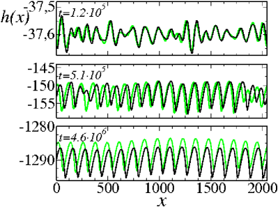
Figure 2: (color online) Height profiles at different times given by the 1D two-field model (black line) for parameters as in Fig. 1 and by the effective equation [Eq. (44)] (green line) with parameters as given by relation (45), namely, $v_{0}=-3\cdot 10^{-4}$, $\gamma_{x}=3\cdot 10^{-4}$, $\nu_{x}=-9\cdot 10^{-3}$, $\lambda_{x}^{(1)}=9\cdot 10^{-4}$, $\Omega_{x}=-0.297$ , $\xi_{x}=3\cdot 10^{-4}$, $\mathcal{K}_{xx}=1.0993$, and $\lambda^{(2)}_{xx}=0.8901$. All units are arbitrary.

We can see how, starting from the same flat random initial distribution for both systems, a periodic surface structure appears with a wavelength of about the maximum of the linear dispersion relation, and the amplitude of height variations increases. For the examples considered in Fig. 2 the wavelength of the linear instability is given by (27), yielding ${l}^{\ell}=98$. At these short times, when the slopes are not too large so that nonlinear terms are not yet relevant, both profiles match quite accurately. Far from the linear instability threshold, the profiles become less similar. Since the space and time scales separation and the power expansion performed to obtain the effective equation are only valid for small values of $\epsilon$, it is expected that, the smaller $\epsilon$ is, the more similar the profiles become. However, if we reduce this parameter, the simulations are more time consuming since the characteristic space and time scales for pattern dynamics are inversely proportional to powers of $\epsilon$, as noted in Sec. IV. In any case, for the values of $\epsilon$ considered in our simulations, the effective equation captures the main features of the original two-field model, even in terms of the behavior of observables such as the global surface rms width or roughness $W(t)$ or the ripple wavelength $l(t)$ (defined as the mean lateral distance between two consecutive local minima), as seen in Figs. 3 and 4, respectively.

V.3 Nonlinear dynamics for the effective equation

Indeed, at later stages, nonlinearities determine the evolution of the surface morphology. For the reasons mentioned above, we will explore this regime through the effective interface equation. Specifically, nonlinear effects induce coarsening of structures wherein the cells (ripples) grow in width and height, their number decreasing in both systems. For both cases coarsening is such that smaller cells are “eaten” by larger neighbors until reaching constant amplitude and wavelength values, while lateral moundlike order is still preserved for intermediate distances (more than ten times the lateral size of the cells). This behavior is very similar to that reported in Ref. [Muñoz-García et al., 2006b] for the mixed KS equation equation that corresponds to the $\gamma_{x}=\Omega_{x}=\xi_{x}=0$ limit of (44); see also paper II.

In Figs. 3 and 4 we show the time evolution of the surface roughness $W(t)$ and ripple wavelength ${l}(t)$, averaged over 18 random initial conditions. After a stage in which the amplitude of the linear instability and, therefore $W$, grow exponentially, a coarsening process begins (roughly at $t\simeq 3\cdot 10^{5}$) for the ripple wavelength. Around $t=2\cdot 10^{6}$ this process stops and the wavelength and amplitude of the pattern reach stationary values. Specifically, the lateral pattern wavelength grows from its initial value corresponding to the linear instability ${l}^{\ell}=98$ until a saturation value, close to ${l}=121$. At intermediate times this coarsening behavior can be described by an effective power law ${l}\sim t^{0.12}$, as suggested in Fig. 4. In the presence of coarsening, the dependence of the asymptotic values of the ripple amplitude and wavelength with system parameters differs from those of the linear instability regime. If one assumes Csahók et al. (2000) that the odd-derivative terms in Eq. (44) do not contribute to such a coarsening process, approximate values can be obtained through comparison with coarsening dynamics in the conserved KS equation.Muñoz-García et al. (2006b) Such estimates are more accurate in the normal incidence case (paper II),Muñoz-García et al. (2008) to which we refer the interested reader.

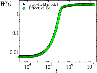
Figure 3: (color online) Temporal evolution of the global roughness, $W(t)$ given by the two-field model (blue triangles) and by the effective interface equation (green circles) for the same coefficients as in Fig. 2. Error bars are smaller than the symbol sizes. All units are arbitrary.

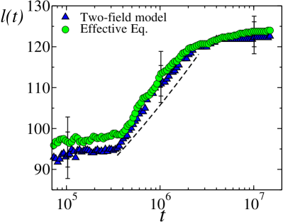
Figure 4: (color online) Temporal evolution of the lateral pattern wavelength, ${l}(t)$, given by the two-field model (blue triangles) and by the effective interface equation (green circles) for the same coefficients as in Fig. 2. A few representative error bars are given that represent statistical dispersion. The dashed line corresponds to ${l}(t)\sim t^{0.12}$. All units are arbitrary.

Additional important features of these systems, which are not present in the equation studied in Ref. [Muñoz-García et al., 2006b], are the asymmetry of the profile and the lateral movement of the pattern. As we have checked in our simulations, the asymmetry on the pattern depends only on the (advective) terms corresponding to the coefficients $\Omega_{x}$ and $\xi_{x}$ of the effective equation. For negative values of $\Omega_{x}$ and/or positive values of $\xi_{x}$ the cell structure tends to be leaning to the right. This can be observed in Figs. 1 and 2, where the right slopes of the cells are clearly larger than the left slopes. If $\Omega_{x}$ is positive and/or $\xi_{x}$ is negative, the pattern is leaning to the left. If both terms have the same sign, the orientation of the structure depends on their relative magnitude.

Considering lateral ripple motion, note first that the linear prediction for the velocity, Eq. (29) has the form $V^{\ell}=-\gamma_{x}+4\pi^{2}\Omega_{x}({l}^{\ell})^{-2}$. The contribution due to $\gamma_{x}$ is an uniform translation (along a direction on the $x$ axis that is opposite to the sign of $\gamma_{x}$) that can actually be cancelled out by an appropriate choice of reference frame. Thus, the only remaining terms which influence in-plane displacement of the pattern are again $\Omega_{x}$ (linear) and $\xi_{x}$ (non-linear). For the values we have considered for the remaining parameters, a positive sign of $\Omega_{x}$ and/or $\xi_{x}$ induces ripple motion towards positive $x$, while negative values of these parameters lead to lateral ripple motion in the opposite direction. In Fig. 5 we observe the lateral movement of the pattern as described by Eq. (44), for parameters as in Fig. 2. Simultaneously with erosion and mean height evolution towards larger negative values, the pattern is moving towards the left. Here, the movement is dominated by $\gamma_{x}$ and $\Omega_{x}$, which induce motion towards the negative $x$ values.

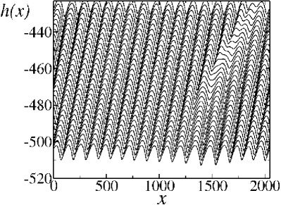
Figure 5: Height profiles between $t=1.5\cdot 10^{6}$ (top) and $t=1.8\cdot 10^{6}$ (bottom) evaluated at equally spaced intervals of $10^{4}$ time units, for the effective equation (44), and parameters as in Fig. 2. All units are arbitrary.

The results reported in this section allow us to conclude that both the effective interface equation and the two field model, whose coefficients are related through (45), capture common features observed in experiments such as the coarsening process of the pattern wavelength, the short range lateral order and the non uniform lateral displacement of the structure. On the other hand, due to the fact that the scales associated with the experimental linear instability are very large (of the order of $\epsilon^{-1/2}$), one needs very large simulations in order to compare with experiments. These are available to the effective equation, in which parameters can be rescaled with the aim of accelerating the simulations. For these reasons, in going to the physical 2D case in the next section, we will limit our study to the 2D effective height equation (42). We will consider some illustrative examples of the ensuing surface dynamics that allow us to understand the richness of the behaviors that can be described by such a complex non-linear system.

VI Full 2D effective interface equation

Equation (42) generalizes the one-dimensional equation (44) to the case of fully anisotropic two-dimensional targets, in a way that is consistent with reflection symmetry in the $y$ direction, as expected from the ion incidence geometry. As mentioned earlier, Eq. (42) generalizes the one-field equation (55), through appearance here of the (anisotropic) conserved-KPZ type terms $\partial_{i}^{2}(\partial_{j}h)^{2}$. In turn, Eq. (55) already provided an anisotropic generalization (through the presence of odd derivatives in the $x$ coordinate) of the two-dimensional KS equation.Cuerno and Barabási (1995); Rost and Krug (1995) To the best of our knowledge, Eq. (42) is new and adds to the relatively small number Bar and Nepomnyashchy (1995) of (local) evolution equations for fully anisotropic two-dimensional pattern forming systems, that are derived from constitutive laws. In the context of hydrodynamic models of ripple formation on aeolian sand dunes, an isotropic 2D equations, when available, are limited to conservative dynamics,Yizhaq et al. (2004) while in the cases of thin film surfaces nonlinearities that arise are of a different type.Sato and Uwaha (1999); Golovin et al. (1999); Levandovsky et al. (2006)

Although the parameter space of Eq. (42) is much larger than that of its one-dimensional counterpart (44), the physical interpretation of the various terms and coefficients is completely analogous, corresponding to a natural generalization of those appearing in the latter. Given that the main linear features of the two-dimensional equation were already discussed (and compared with typical experimental data) in Sec. III.2.2, we next consider numerical simulations of Eq. (42) that show the main morphological features of its full dynamics, that will be later compared with experimental results. Some peculiarities on the cancellation modes that may arise in Eq. (42) are considered analytically in a specific subsection.

VI.1 2D dynamics: numerical results

Far from a complete analysis of Eq (42), we will limit ourselves in this section to a qualitative study of its main properties and how it successfully reproduces some experimental features which are not included in previous continuum descriptions.

Thus, we have performed a numerical integration of Eq. (42) using an scheme that generalizes that employed in the one-dimensional case, namely, an Euler updating rule with $\delta t=10^{-3}$ for the time evolution, and the finite difference prescription of [Lam and Shin, 1998] for the nonlinear terms, with $\delta x=1$. The standard size of our simulations was $L\times L=256\times 256$ with periodic boundary and random initial conditions. We consider a reference plane comoving with the eroded surface with a constant velocity $-v_{0}$, thus the effective equation that we integrate is (42) for $v_{0}=0$.

The evolution of the height as described by Eq. (42) is depicted in Figs. 6-8 for different values of the coefficients, with the $x$-axis oriented along the horizontal direction (see also supplementary videos).EPA (a, b, c) In each figure three snapshots (top views and lateral cuts) are provided for a given parameter condition, with time increasing from panel (a) to panel (c). In all these examples, and resembling experimental morphologies,Muñoz-García et al. (in press. arXiv:0706.2625v1) both the amplitude and the wavelength of the ripples grow with time, while the pattern disorders in heights for long lateral distances. The detailed shapes of the topographies, however, are quite different depending on the values of the parameters. We can obtain longitudinally disordered ripples which are frequently interrupted along the direction of the crests, as in Fig. 6, or else ordered straight and wide ripples occur for different parameter conditions as in Fig. 7. An even more disordered pattern is depicted in Fig. 8, where the ripples group into domains of about three cells whose crests run along the $x$ axis, as expected from the parameter values (note $\nu_{x}>0$ in this example).

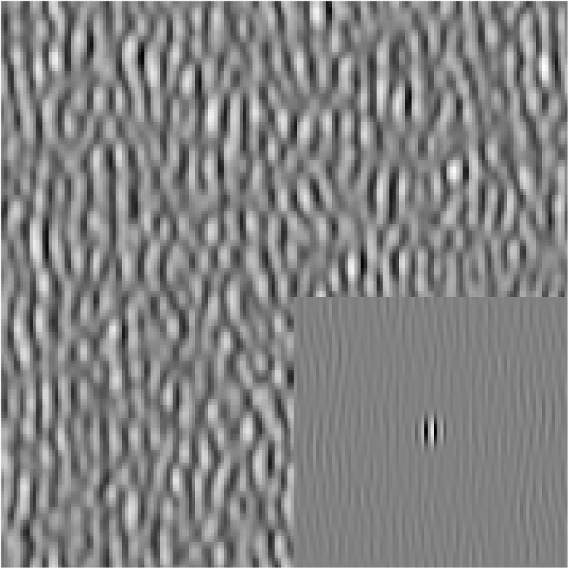
(a)

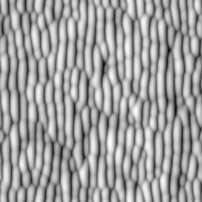
(b)

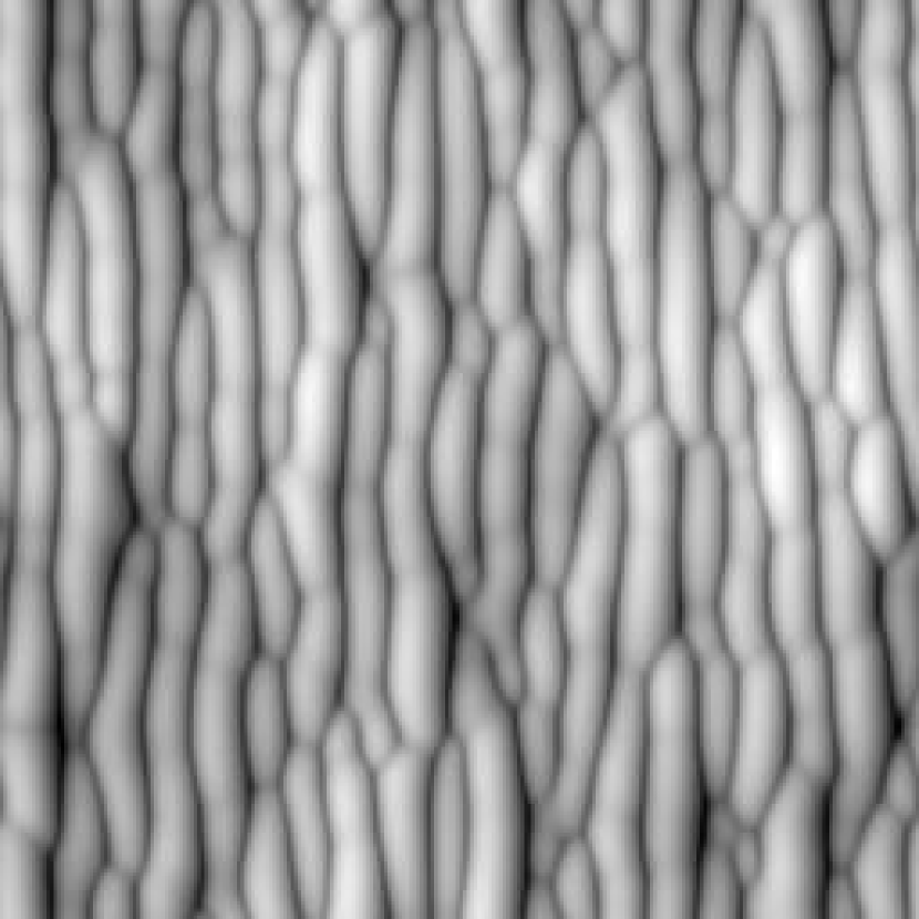
(c)

Figure 6: Time evolution of relatively disordered ripples with mild wavelength coarsening (see also supplementary video).EPA (a) Snapshots at increasing times: (a) $t=10$; (b) $t=106$; (c) $t=953$ for Eq. (42) with $v_{0}=0$, $\gamma_{x}=-0.1$, $\nu_{x}=-1$, $\nu_{y}=-0.1$, $\Omega_{x}=1$, $\Omega_{y}=0.5$, $\xi_{i}=0.1$, $\lambda_{x}^{(1)}=1$, $\lambda_{y}^{(1)}=5$, $\lambda^{(2)}_{i,j}=5$, and ${\cal K}_{i,j}=1$. Top views (left column) and corresponding transverse cuts at $y=L/2$ (right column). Inset in (a) is its corresponding height autocorrelation. All units are arbitrary.

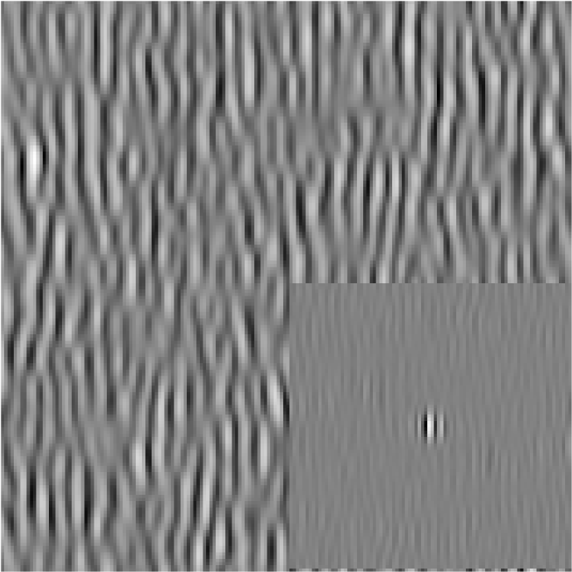
(a)

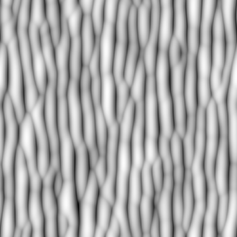
(b)

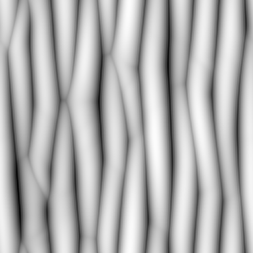
(c)

Figure 7: Time evolution of relatively ordered ripples with sizeable wavelength coarsening (see also supplementary video).EPA (b) Snapshots at increasing times: (a) $t=10$; (b) $t=106$; (c) $t=953$ for Eq. (42) with the same parameters as in Fig. 6, except for $\lambda_{x}^{(1)}=0.1$. Top views (left column) and corresponding transverse cuts at $y=L/2$ (right column). Inset in (a) is its corresponding height autocorrelation. All units are arbitrary.

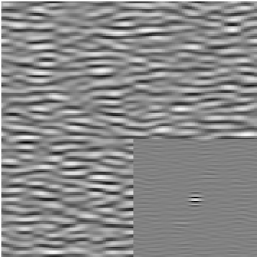
(a)

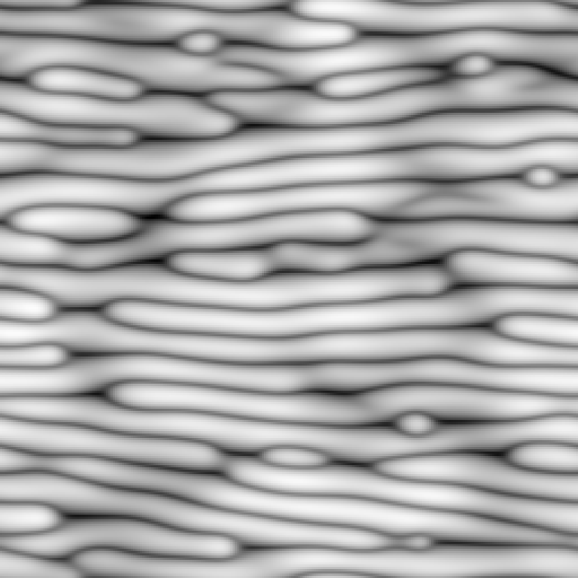
(b)

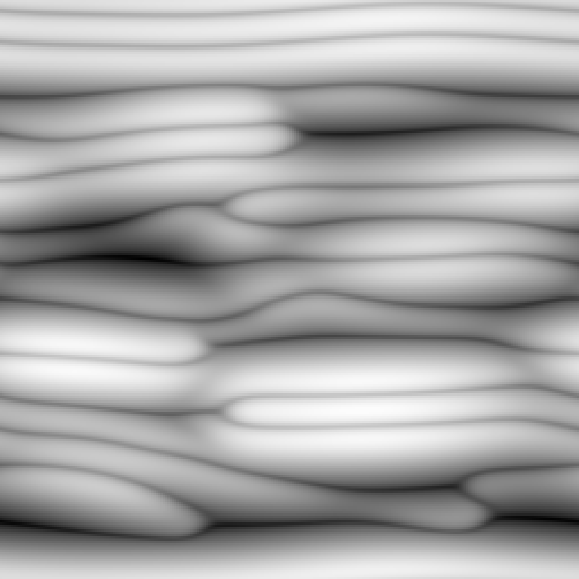
(c)

Figure 8: Time evolution of relatively disordered ripples with sizeable wavelength coarsening (see also supplementary video).EPA (c) Ripple orientation as for typical large incidence angle conditions. Snapshots at increasing times: (a) $t=10$; (b) $t=106$; (c) $t=953$ for Eq. (42) with $v_{0}=0$, $\gamma_{x}=0.1$, $\nu_{x}=1$, $\nu_{y}=-0.95$, $\Omega_{i}=-0.5$, $\xi_{i}=0.1$, $\lambda_{x}^{(1)}=0.1$, $\lambda_{y}^{(1)}=1.0$, $\lambda^{(2)}_{i,x}=0.5$, $\lambda^{(2)}_{i,y}=5.0$, and ${\cal K}_{i,j}=1$. Top views (left column) and corresponding transverse cuts at $x=L/2$ (right column). Inset in (a) is its corresponding height autocorrelation. All units are arbitrary.

Similarly to the one-dimensional case, before slopes are large enough to make non-linear terms non-negligible, the evolution of the morphology is governed by linear terms. This will allow us to separate the dynamics into two different regimes, linear and nonlinear, according to the type of terms that control the evolution.

VI.1.1 Linear regime

As noted in Sec. IV, the linear dispersion relation of Eq. (42) coincides with that of the original model described in subsection III.2. Thus, for isotropic thermal surface diffusion, the ripple crests are oriented along the $y$ ($x$) axis if $\nu_{x}$ ($\nu_{y})$ is more negative than $\nu_{y}$ ($\nu_{x}$), thus reproducing the ripple orientation as predicted by the BH theory. Numerical integration within linear regime indeed retrieves the dependence of the ripple orientation as a function of the values of $\nu_{x}$ and $\nu_{y}$ as shown in Figs. 6, 7, and 8. Furthermore, we have also checked in our simulations that the lateral wavelength of the pattern is given by the relation between the surface tension and diffusion terms. One way to do that is to measure the distance from the origin to the first maximum in the height autocorrelation function which is represented in the inset of Figs.  6(a), 7(a), and 8(a). Since ${\mathcal{K}}_{ij}=1$ is considered for all these examples, we have ${l}^{\ell}=2\pi/k^{\ell}_{i}=2\pi(-2/\nu_{i})^{1/2}$.

While even linear derivatives in Eq. (42) are responsible for amplification or attenuation of the ripple amplitude, they do not induce lateral motion of pattern. Conversely, odd derivatives breaking the $x\rightarrow-x$ symmetries indeed induce in-plane lateral ripple motion. We have checked in our simulations that, as expected, the term corresponding to the coefficient $\gamma_{x}$ does not alter the shape of the morphology but merely produces a uniform movement along the $x$ axis. As in the one-dimensional case, the direction of this movement is opposite to the sign of $\gamma_{x}$. On the other hand, again as in the 1D case, the $\Omega_{i}$ terms are responsible for both lateral movement of the structure and shape asymmetry. These effects can be observed in Fig. 9 where we show the time evolution (as seen from a comoving reference frame) of transverse cuts of the surface for a given parameter condition. We have checked that, indeed, transforming back to a rest reference frame, the ripple velocity coincides, for times within linear regime, with that predicted by Eq. (29). Already visual inspection of Fig. 9 suggests deviations from a uniform velocity for transverse ripple motion. This is a signature of nonlinear effects [specifically, due to ripple coarsening manifested by a non constant ripple wavelength ${l}(t)]$, that are considered next.

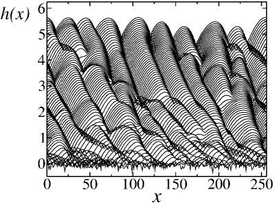
Figure 9: In-plane non-uniform ripple motion as seen from the evolution of transverse cuts of the surface at $y=L/2$ for equally spaced times between $t=0$ and $t=1500$. Results from the numerical integration of Eq. (42) with $v_{0}=0$, $\nu_{x}=-1$, $\nu_{y}=-0.1$, $\gamma_{x}=\xi_{i}=0$, $\Omega_{i}=-2$, $\lambda_{x}^{(1)}=1$, $\lambda_{y}^{(1)}=5$, $\lambda^{(2)}_{i,x}=50$, $\lambda^{(2)}_{i,y}=5.0$, and ${\cal K}_{i,j}=1$. All units are arbitrary.

VI.1.2 Non-linear regime

For long enough times, non-linear terms have to be considered in order to understand the evolution of the morphology. Those containing even derivatives are reflection symmetric in $x$ and, therefore, are not responsible for lateral movement or any asymmetries of the pattern. On the other hand, we have checked that the terms corresponding to the coefficients $\xi_{i}$ indeed induce lateral motion of the pattern and asymmetry in the $x$ axis. For the parameters considered in our simulations, positive values of $\xi_{i}$ induce a non-uniform lateral motion of the pattern towards positive $x$ values. Since the contributions of the $\xi_{i}$ nonlinearities to the evolution of $h$ increase in the non-linear regime, these can even induce a change in the direction of the pattern movement as observed in Fig. 10, where we plot the time evolution of a transverse cut of the surface. In this figure $\Omega_{i}=-2<0$, thus, as noted in the previous subsection, this induces a movement of the pattern towards negative $x$. These terms dominate during the linear regime but, as a result of the increase of the values of lower order surface derivatives, the $\xi_{i}=4.5>0$ terms take over and change the direction of lateral ripple motion towards positive $x$ values. This example underscores the complex ripples dynamics induced by nonlinear effects, that should be taken into account in the discussion of the potential limitations of the current BH picture to quantitatively describe ripple motion.Chan and Chason (2007); Alkemade (2006)

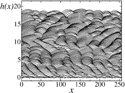
Figure 10: Change in the direction of in-plane ripple motion as seen from the evolution of transverse cuts of the surface at $y=L/2$ for equally spaced times between $t=0$ and $t=5000$. Results from the numerical integration of Eq. (42) for parameters as in Fig. 9 except for $\xi_{i}=4.5$. All units are arbitrary.

A simpler type of non-uniform ripple motion that has been reported experimentally corresponds to movement in a fixed direction, but with a non-uniform velocity, see $e.g.$ [Habenicht et al., 2002; Alkemade, 2006]. As mentioned above, this behavior correlates with the occurrence of wavelength coarsening (see below), and Eq. (42) is the first two-dimensional continuum equation to describe it within the IBS context. As an example, in Fig. 11 we show the (non-uniform) ripple velocity $V(t)$ in the non-linear regime as a function of time for the same simulations as shown in Fig. 9. Here the velocity is computed for a single surface minimum once the pattern is completely formed. At longer times the ripple velocity seems to reach a negligible value compatible with arrest of ripple motion. This might be related with a similar interruption of ripple coarsening that is illustrated below.

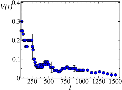
Figure 11: (color online) Temporal evolution of the lateral ripple velocity, $V(t)$, given by the numerical integration of Eq. (42) in the non-linear regime for the same coefficients as in Fig. 9. A few representative error bars are given. All units are arbitrary.

Non-linear terms containing derivatives that are reflection-symmetric in $x$ are responsible for the eventual saturation of the ripple amplitude, and for the quality and range of in-plane order of the ripple pattern. As checked in our simulations and described for the 1D effective equations studied in Sec. V.2 and [Muñoz-García et al., 2006b], the larger the value of the ratio of $\lambda^{(2)}_{i,j}$ to $\lambda^{(1)}_{i}$ terms is, the longer is the coarsening process, and the more ordered the morphology becomes for the same total time ($i.e.$, ion dose). This is shown in Figs. 12 and 13, in which the time evolution of the global surface roughness and of the lateral wavelength of the pattern are depicted for different values of this ratio, denoted as $r$. In general, the roughness increases exponentially (linear instability regime), after which the nonlinearities are able to stabilize the system and induce slower growth for the roughness, $W(t)$ finally reaching a time independent value. For very small $r$ ratios, this stationary state seems to be reached earlier, and the intermediate slow (power-law) growth regime of the roughness is shorter. For larger values of $r$, this intermediate regime has a wider duration, and can be more accurately described by a power law with the form $W(t)\sim t^{\beta}$ for some effective value of the growth exponent $\beta$. Note that, in the $r\to\infty$ limit (equivalently, $\lambda^{(1)}_{i}$ = 0), Eq. (42) does not seem to have a stationary state, similarly to the conserved KS equation.Raible et al. (2000); Muñoz-García et al. (2006b) Note, the growth exponent for this case is Raible et al. (2000) $\beta_{\rm cKS}=1$. The gradual chan ge of the duration of this intermediate power-law regime with physical parameters (that enter the value of the ratio $r$) and the different values for the effective growth exponent that can be obtained when trying to fit a power-law to such type of data, may account for the spread in the related growth exponents experimentally reported in the context of ripple formation (see references in [Chan and Chason, 2007; Muñoz-García et al., in press. arXiv:0706.2625v1]).

Regarding the quality and range of order in the ripple pattern at intermediate and long times, Fig. 12 already shows that the morphology is more disordered (the roughness is larger) for smaller values of $r$. Moreover, for these cases, as seen in Fig. 13, the stationary value of the pattern wavelength is smaller, and is achieved earlier. A qualitatively similar behavior has been experimentally found in IBS of silicon targets under normal incidence conditions.Gago et al. (2006) Note, the standard one-field continuum equation (55) corresponds to the $r=0$ limit, for which there is no coarsening and the system is roughest (the roughness being larger almost by an order of magnitude, as seen in Fig. 12). Hence, such an equation was not able to account for the observed ripple coarsening and improved ordering, in marked contrast with the present Eq. (42). As in the case of the roughness, for the opposite cKS-type limit $r\to\infty$ ($\lambda^{(1)}_{i}=0$), the ripple wavelength does not reach a stationary value. Rather, both the amplitude and ${l}(t)$ increase indefinitely, similarly to the cKS case for which ${l}(t)_{\rm cKS}\sim t^{0.5}$, until a single ripple (with a parabolic cross-section) remains in a finite system.Raible et al. (2000)

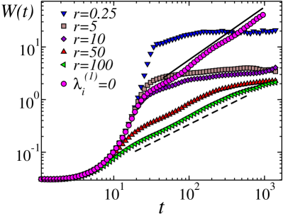
Figure 12: (color online) Temporal evolution of the global roughness, $W(t)$, given by the the effective equation Eq. (42) with $v_{0}=0$, $\nu_{x}=-1$, $\nu_{y}=-0.1$, $\gamma_{x}=\xi_{i}=\Omega_{i}=0$, ${\cal K}_{i,j}=1$, $\lambda_{i}^{(1)}=0.1$, and $\lambda^{(2)}_{i,j}=0.1r$, for different values of $r$. The solid and dashed lines show the fit to power laws for $\lambda_{i}^{(1)}=0$ and $r=100$ where $W\sim t^{1.00}$ and $W\sim t^{0.71}$, respectively. All units are arbitrary.

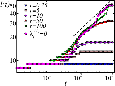
Figure 13: (color online) Temporal evolution of the lateral wavelength of the pattern, ${l}(t)$, given by the effective equation Eq. (42) for the same coefficients as Fig. 12. The dashed line shows the fit to a power law for $r=100$ where ${l}\sim t^{0.38}$. The fit in the same region for $\lambda_{i}^{(1)}=0$ yields ${l}\sim t^{0.48}$ (not shown). All units are arbitrary.

Results obtained for the one dimensional anisotropic equation (44) and for the 1D and 2D isotropic counterparts Muñoz-García et al. (2006b, 2008) lead us to expect disorder to dominate the morphological features at the largest length and time scales in the system, as long as cancellation modes do not arise (namely, as long as $\lambda^{(1)}_{x}$ and $\lambda^{(1)}_{y}$ have the same signs, see next section). Thus, we expect scale invariant morphologies and rough surfaces for much larger distances than the pattern wavelength. The statistics of the surface fluctuations at these scales are expected to be characterized by the critical exponents of some of the universality classes of kinetic roughening.Barabási and Stanley (1995) However, the case of the isotropic KS equation not being even completely understood,Boghosian et al. (1999) we can only conjecture, by analogy with the 1D case, that the asymptotic scaling of Eq. (44) is in the 2D KPZ universality class.

VI.1.3 Cancellation Modes

Eq. (42) can display cancellation modes (CM), analogously to its own 1D counterpart, Eq. (44), and to the anisotropic KS (aKS) equation.Rost and Krug (1995); Park et al. (1999) Recall that CM in Eq. (44) arise due to cancellation between the nonconserved $(\partial_{x}h)^{2}$ and the conserved $\partial^{2}_{x}(\partial_{x}h)^{2}$ KPZ nonlinearities, and lead to (possibly) finite time blow-up of the solutions to the differential equation. We will refer to these as mixed KS (mKS) CM. In marked contrast, CM in the aKS system appear only when the coefficients of the two nonlinear terms $\lambda^{(1)}_{x}$ and $\lambda^{(1)}_{y}$ have different signs, and lead to a long time ripple pattern that is oriented along an oblique direction in the $xy$ plane,Rost and Krug (1995); Park et al. (1999) the system apparently supporting such type of solution for long times. We will denote these as aKS CM.

Given the large parameter space of Eq. (42), the two types of CM mentioned can arise, and we consider separately the conditions for appearance of each of them. Notice, it suffices to consider the nonlinearities that are reflection symmetric in $x$, as they are the only ones involved in the evolution (and putative blow up) of the ripple amplitude.

mKS-type CM.

The nonconserved and conserved KPZ nonlinearities in Eq. (42) read explicitly

$${\cal N}[h] \equiv \lambda^{(1)}_{x}(\partial_{x}h)^{2}+\lambda^{(1)}_{y}(\partial_{y}h)^{2}-\lambda^{(2)}_{xx}\partial^{2}_{x}(\partial_{x}h)^{2}$$

$$-\lambda^{(2)}_{xy}\partial^{2}_{x}(\partial_{y}h)^{2}-\lambda^{(2)}_{yx}\partial^{2}_{y}(\partial_{x}h)^{2}-\lambda^{(2)}_{yy}\partial^{2}_{y}(\partial_{y}h)^{2},$$

whose Fourier transform reads

$${\cal F}({\cal N}[h])=Q_{x}{\cal F}[(\partial_{x}h)^{2}]+Q_{x}{\cal F}[(\partial_{y}h)^{2}],$$ (50)

where we have defined

$$Q_{x} = \lambda^{(1)}_{x}+\lambda^{(2)}_{xx}k_{x}^{2}+\lambda^{(2)}_{yx}k_{y}^{2},$$ (51)

$$Q_{y} = \lambda^{(1)}_{x}+\lambda^{(2)}_{xy}k_{x}^{2}+\lambda^{(2)}_{yy}k_{y}^{2}.$$ (52)

Now, using (43), we get

$$Q_{i}=\lambda^{(1)}_{i}\left(1+\frac{\Delta}{\phi}k^{2}\right),$$ (53)

where we have assumed isotropy in the surface tension coefficients as done in Appendix C, $\gamma_{2x}=\gamma_{2y}=\gamma_{2}$, and introduced $\Delta=\bar{\phi}D/\gamma_{0}-\phi R_{eq}\gamma_{2}$. As a function of system parameters, there are two possibilities:

• If $\Delta\geq 0$, then $Q_{x},Q_{y}\neq 0$, so that there are no cancellations among nonconserved and conserved KPZ terms along any direction. This is the 2D generalization of the analogous 1D condition discussed in Section V.1.2.

• If $\Delta<0$, then cancellation occurs simultaneously in the $x$ and $y$ directions, for all Fourier modes on the circle $|k_{mKS}|=(\phi/|\Delta|)^{1/2}$, and we expect the solutions of Eq. (42) to diverge for long times. However, as long as we are close to the instability threshold, the putative CM [being $k_{mKS}\sim O(1)$] are outside the band of linearly unstable modes, so that no divergence occurs and Eq. (42) still provides a mathematically well-defined model.

aKS-type CM.

Even in the most favorable case ($\Delta\geq 0$) considered in the previous discussion, there is still the possibility that cancellation takes place, not between nonlinearities of different order (mKS type) but, rather, for specific directions on the $xy$ plane, as in the aKS type. In order to assess such a possibility, we make the Ansatz Rost and Krug (1995) that solutions are of the form $h(x,y,t)=f(x-uy,t)$, and see how this reflects into the KPZ nonlinearities (VI.1.3). Thus,

$${\cal N}[h]=(\lambda^{(1)}_{x}+u^{2}\lambda^{(1)}_{y})\left\{(f^{\prime})^{2}-\frac{\Delta(1+u^{2})}{\phi}[(f^{\prime})^{2}]^{\prime\prime}\right\},$$ (54)

where primes denote differentiation of $f$ with respect to its first argument. As a consequence, exactly as in the aKS case, whenever the coefficients of the nonconserved KPZ nonlinearities, $\lambda^{(1)}_{x}$ and $\lambda^{(1)}_{y}$, have different signs (as a result of their dependence on physical parameters), cancellation takes place for a Fourier mode that is oriented at an angle $\tan^{-1}(-\lambda^{(1)}_{x}/\lambda^{(1)}_{y})^{1/2}$ with the $x$ axis. Actually, for an appropriate choice of the function $f$ additional cancellation may take place irrespective of the signs of the $\lambda^{(1)}_{i}$ coefficients, but such special cases are not generic. In Fig. 14 we show an example of the evolution of the morphology in case of cancellation modes oriented at $45^{\circ}$ to the $x$ axis.

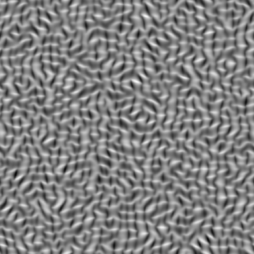
$t=25$

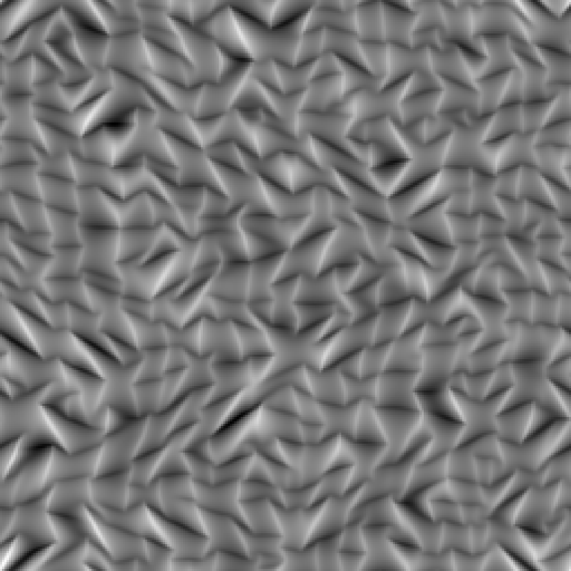
$t=50$

$t=185$

Figure 14: Long time development of oblique ripple patterns at $45^{\circ}$ to the $x$ axis due to cancellation modes (see text). Top views of morphologies obtained by numerical integration of Eq. (42) with $v_{0}=0$, $\nu_{x}=-1$, $\nu_{y}=1$, $\gamma_{x}=\xi_{i}=\Omega_{i}=0$, ${\cal K}_{i,j}=1$, $\lambda_{x}^{(1)}=0.1$, $\lambda_{y}^{(1)}=-0.1$, $\lambda^{(2)}_{i,x}=0.5$, and $\lambda^{(2)}_{i,y}=-0.5$ at increasing times. All units are arbitrary.

It is tempting to interpret the obliquely oriented ripples recently found Ziberi et al. (2008) on Si at 2 keV as some type of cancellation mode of this aKS type.

VI.2 2D dynamics: comparison to experiments

Along the discussion on the detailed surface dynamics predicted by Eq. (42), we have already pointed out relation to experimental features that are described by this new effective equation. In our discussion, we have assumed as a reference case that dependencies of coefficients $\alpha_{ikj}$ on the physical parameters such as average ion energy and flux, temperature, and characteristics of the distribution of energy deposition in the target, are as in BH-type approaches for amorphizable targets. Within such an assumption, all dependencies of linear features on the latter are as in one-field models,Makeev et al. (2002) whose comparison to experiments has been reviewed in detail elsewhere.Makeev et al. (2002); Valbusa et al. (2002); Chan and Chason (2007); Muñoz-García et al. (in press. arXiv:0706.2625v1) Whenever discrepancies arise, some may be due to deviations of the actual collision cascade statistics from Sigmund’s Gaussian formula, and this is a matter of current active research.Feix et al. (2005); Davidovitch et al. (2007)

There are other features of our two-field model and of the ensuing Eq. (42), that seem more robust to modifications in the values of the parameters entering $\Gamma_{ex}$, provided there is a morphological instability in the “surface tension” coefficients. Thus, the formation and fast stabilization of a stationary value for the thickness of the amorphous mobile layer has been assessed $e.g.$ for Si both in Molecular Dynamics Moore et al. (2004) and in experiments, see [Ziberi et al., 2005] or [Chini et al., 2003] (for energies of tens of keV). Asymmetry in ripple cross sections has also been assessed both by microscopy (for Si, see [Ziberi et al., 2005]) or by techniques in reciprocal space ($e.g.$ sapphire Zhou et al. (2007)). Also wavelength coarsening has been profusely documented, there being a large spread in the values of the effective coarsening exponents, see references in [Muñoz-García et al., in press. arXiv:0706.2625v1] and more recently $e.g.$ [Katharria et al., 2007] for SiC. As for in-plane ripple motion, there is a smaller number of studies, although detailed studies (typically employing focused ion beams) are indeed available Habenicht et al. (2002) for Si and for glass,Alkemade (2006) the phenomenon having been reported also in atomistic simulations of amorphous carbon targets.Koponen et al. (1997)

VII CONCLUSIONS

In this paper we have considered in detail a two-field continuum description of nanopatterning by IBS in the the most general (anisotropic) case of oblique ion incidence. The explicit coupling of the dynamics for diffusing species at the surface with the evolution of the topography assumes exchange between mobile and immobile material at the upper boundary of the latter. This description goes beyond the IBS case and can be employed as a phenomenological formulation of more general phenomena in Surface Science. In the particular case of IBS, this approximation leads to a stationary value for the density of diffusing surface species that is very quickly reached at, as compared with the dynamics of the surface morphology. This fact and the shape of the effective interface equation are robust to the specifics of the distribution of energy deposition, while these reflect in the values of the model parameters. For the sake of reference, in this work we have been assuming BH behavior for the latter. Under this assumption, we have explored the qualitative properties of the two-field model, and seen that it indeed provides a more comprehensive framework than previous continuum descriptions fulfilling most of the desiderata formulated in the Introduction. The adoption of a two-field description is not for mere mathematical convenience; rather, it responds to its enlarged set of physical mechanisms (such as redeposition) entering the constitutive laws in a more natural way ($e.g.$ the coupling between excavation and surface transport, or corrections to BH prediction for the linear velocity of transverse ripple motion). The parameter range for cancellation modes is partially restricted, and important experimentally observed nonlinear behavior, such as wavelength coarsening and non-uniform ripple motion, can be accounted for. Analogous conclusions can be reached at in the cases of normal incidence, or oblique incidence onto rotating targets, that are considered in detail in a forthcoming work.Muñoz-García et al. (2008)

Still, some features that remain theoretically unexplained, such as $e.g.$ the lack of pattern formation for IBS of Si at near normal incidence in many experimental settings, may be due to inaccuracies in Sigmund’s description of the statistics of energy deposition through collisions inside the target.Davidovitch et al. (2007) Note that, once these are improved upon, the resulting effective parameters could be used in turn as inputs for the local excavation rate (3). Thus, the two-field model is not restricted in principle to Sigmund’s Gaussian statistics. Moreover, through the mentioned natural coupling between transport and topography, and through the incorporation of redeposition effects, it already provides (albeit, admittedly, in a simplified form that is susceptible to refinement) description of additional material rearrangement due to ion impingement, that currently seems necessary for a theoretical description of IBS with an improved predictive power.Kalyanasundaram et al. (2008)

Appendix A Sigmund’s energy distribution

In [Makeev et al., 2002], the most general equation of motion for the local surface velocity reads

$$\partial_{t}h=-v_{0}+\gamma_{x}\partial_{x}h+\Omega_{1}\partial^{3}_{x}h+\Omega_{2}\partial_{x}\partial_{y}^{2}h\\ +\left[\xi_{x}\left(\partial_{x}h\right)+\nu_{x}\right]\left(\partial^{2}_{x}h\right)+\left[\xi_{y}\left(\partial_{x}h\right)+\nu_{y}\right]\left(\partial^{2}_{y}h\right)\\ -D_{xx}\partial^{4}_{x}h-D_{yy}\partial^{4}_{y}h-D_{xy}\partial^{2}_{x}\partial_{y}^{2}h+\frac{\lambda_{x}}{2}\left(\partial_{x}h\right)^{2}+\frac{\lambda_{y}}{2}\left(\partial_{y}h\right)^{2},$$ (55)

where all coefficients are functions Makeev et al. (2002) of physical parameters such as $\theta$, $E$, $\Phi$, and the characteristics of Sigmund’s Gaussian energy distribution, such as the average penetration depth, $a$, and the lateral widths of the distribution $\sigma$ and $\mu$. In particular, the coefficients $D_{ij}$ correspond to the so-called ion-induced effective smoothing terms whose terms have the same shape as those characteristic of surface diffusion, but are of a mere “geometric” origin related with describing the surface height at sufficiently high order in a Taylor expansion in height derivatives. For this (standard) choice, the values of coefficients $\alpha_{ikl}$ in the excavation rate $\Gamma_{ex}$ in (3) are

$$\alpha_{0} =v_{0},\quad\alpha_{1x}=-\gamma_{x}/v_{0},\quad\alpha_{2x,y}=-\nu_{x,y}/v_{0},$$

$$\alpha_{3x} =-\Omega_{1}/v_{0},\quad\alpha_{3y}=-\Omega_{2}/v_{0},\quad\alpha_{4ij}=-D_{ij}/v_{0},$$

$$\alpha_{5x,y} =-\xi_{x,y}/v_{0},\quad\alpha_{6x,y}=-\lambda_{x,y}/v_{0}.$$ (56)

Appendix B Formulae for Sec. III

$$a=\gamma_{0}+\sum_{j=x,y}\left[D+R_{eq}\gamma_{0}\left(\gamma_{2j}-\epsilon\alpha_{2j}+\epsilon\sum_{i=x,y}\alpha_{4ij}k_{i}^{2}\right)\right]k^{2}_{j},$$ (57)

$$b=\epsilon\gamma_{0}R_{eq}k_{x}\left(\alpha_{1x}-\sum_{j=x,y}\alpha_{3j}k_{j}^{2}\right),$$ (58)

$$c=\gamma_{0}R_{eq}D(k_{x}^{2}+k_{y}^{2})\sum_{j=x,y}\left(\gamma_{2j}-\epsilon\alpha_{2j}+\epsilon\sum_{i=x,y}\alpha_{4ij}k_{i}^{2}\right)k_{j}^{2}$$

$$+\epsilon\phi\gamma_{0}^{2}R_{eq}\sum_{j=x,y}\left(-\alpha_{2j}+\sum_{i=x,y}\alpha_{4ij}k_{i}^{2}\right)k_{j}^{2},$$ (59)

$$d=\epsilon\gamma_{0}R_{eq}k_{x}\left[D(k_{x}^{2}+k_{y}^{2})+\phi\gamma_{0}\right]\left(\alpha_{1x}-\sum_{j=x,y}\alpha_{3j}k_{j}^{2}\right).$$ (60)

Appendix C Ripple wavelength and orientation

In this appendix, we determine the ripple orientation and wavelength within linear theory. Our starting point is Eq. (20) which, neglecting $O(\epsilon^{2})$ terms, can be rewritten as

$${\rm Re}(\omega_{\mathbf{k}})=-\nu_{x}k_{x}^{2}-{}\nu_{y}k_{y}^{2}-\mathcal{K}_{xx}k_{x}^{4}-\mathcal{K}_{yy}k_{y}^{4}-\mathcal{K}_{xy}k_{x}^{2}k_{y}^{2},$$ (61)

where

$$\nu_{x} =-\epsilon\phi\gamma_{0}R_{eq}\alpha_{2x},\quad\nu_{y}=-\epsilon\phi\gamma_{0}R_{eq}\alpha_{2y}$$ (62)

$$\mathcal{K}_{xx} =DR_{eq}\gamma_{2x}$$ (63)

$$+\epsilon R_{eq}\gamma_{0}\left[\phi\alpha_{4xx}-\Big{(}\frac{\bar{\phi}D}{\gamma_{0}}-\phi R_{eq}\gamma_{2x}\Big{)}\alpha_{2x}\right],$$

$$\mathcal{K}_{yy} =DR_{eq}\gamma_{2y}$$ (64)

$$+\epsilon R_{eq}\gamma_{0}\left[\phi\alpha_{4yy}-\Big{(}\frac{\bar{\phi}D}{\gamma_{0}}-\phi R_{eq}\gamma_{2y}\Big{)}\alpha_{2y}\right],$$

$$\mathcal{K}_{xy} =DR_{eq}(\gamma_{2x}+\gamma_{2y})+\epsilon R_{eq}\gamma_{0}\Big{[}2\phi\alpha_{4xy}$$ (65)

$$-\left.\frac{\bar{\phi}D}{\gamma_{0}}(\alpha_{2x}+\alpha_{2y})+\phi R_{eq}(\gamma_{2x}\alpha_{2y}+\gamma_{2y}\alpha_{2x})\right].$$

Note that the above $O(k^{4})$ form is a consequence of our long wavelength approximation to $\omega_{\mathbf{k}}$. However, the precise shape of the coefficients is sensitive to the order considered in the (independent) expansion in powers of $\epsilon$, resulting in Eqs. (62)-(65). Thus, for instance, given that $\gamma_{2x}$ and $\gamma_{2y}$ are positive, $\mathcal{K}_{xx}$, $\mathcal{K}_{yy}$, $\mathcal{K}_{xy}$ are also always positive to $O(\epsilon^{0})$. However, the signs of their $O(\epsilon)$ contributions can change with experimental conditions, see $e.g.$ [Makeev et al., 2002].

The experimentally observed pattern is oriented along the direction which yields the maximum value of the real part of the dispersion relation, and its wavelength is associated to the wave vector, $\mathbf{k^{\ell}}=(k_{x}^{\ell},k_{y}^{\ell})$, which maximizes Eq. (61). This vector must verify

$$\frac{\partial{\rm Re}(\omega_{\mathbf{k}})}{\partial k_{x}}\left(\mathbf{k}^{\ell}\right)=\frac{\partial{\rm Re}(\omega_{\mathbf{k}})}{\partial k_{y}}\left(\mathbf{k}^{\ell}\right)=0.$$ (66)

These conditions have the following independent solutions

$$\mathbf{k_{0}} =\left(0,0\right),\,\mathbf{k_{1}}=\left(\sqrt{\frac{{}-\nu_{x}}{2\mathcal{K}_{xx}}},0\right),\,\mathbf{k_{2}}=\left(0,\sqrt{\frac{{}-\nu_{y}}{2\mathcal{K}_{yy}}}\right),$$

$$\mathbf{k_{3}} =\left(\sqrt{\frac{2\nu_{x}\mathcal{K}_{yy}-{}\nu_{y}\mathcal{K}_{xy}}{\mathcal{K}_{xy}^{2}-4\mathcal{K}_{xx}\mathcal{K}_{yy}}},\sqrt{\frac{2{}\nu_{y}\mathcal{K}_{xx}-{}\nu_{x}\mathcal{K}_{xy}}{\mathcal{K}_{xy}^{2}-4\mathcal{K}_{xx}\mathcal{K}_{yy}}}\right).$$ (67)

The solution $\mathbf{k}_{3}$ exists provided the arguments of the square roots of its two components are positive, and $\mathcal{K}_{xy}^{2}-4\mathcal{K}_{xx}\mathcal{K}_{yy}\neq 0$. Otherwise, the only solutions to (66) are $\mathbf{k_{0}}$, $\mathbf{k_{1}}$, and $\mathbf{k_{2}}$. Moreover, as noted above, for large angles of incidence, $\nu_{x}$ is positive and $\mathbf{k_{1}}$ is not defined.

Note, wave vector $\mathbf{k}_{3}$ implies a surface morphology with a periodicity that is aligned neither with the $x$ nor with the $y$ directions (“oblique ripples”). In order to study this solution, we write

$${\rm Re}(\omega_{\mathbf{k_{1}}})-{\rm Re}(\omega_{\mathbf{k_{3}}}) =\frac{\left(\mathcal{K}_{xy}{}\nu_{x}-2\mathcal{K}_{xx}{}\nu_{y}\right)^{2}}{4\mathcal{K}_{xx}\left(\mathcal{K}_{xy}^{2}-4\mathcal{K}_{xx}\mathcal{K}_{yy}\right)},$$ (68)

$${\rm Re}(\omega_{\mathbf{k_{2}}})-{\rm Re}(\omega_{\mathbf{k_{3}}}) =\frac{\left(\mathcal{K}_{xy}{}\nu_{y}-2\mathcal{K}_{yy}{}\nu_{x}\right)^{2}}{4\mathcal{K}_{yy}\left(\mathcal{K}_{xy}^{2}-4\mathcal{K}_{xx}\mathcal{K}_{yy}\right)},$$ (69)

so that the signs of (68), (69) are given by that of

$$\mathcal{K}_{xy}^{2}-4\mathcal{K}_{xx}\mathcal{K}_{yy}.$$ (70)

Moreover, straightforward algebra shows that the sign of the determinant of the Hessian matrix evaluated at $\mathbf{k}=\mathbf{k}_{3}$ is opposite to that of (70). In summary,

1. For positive values of (70), $\mathbf{k}_{3}$ is a saddle point, so that the absolute maximum of (61) takes place either at $\mathbf{k}_{1}$ or at $\mathbf{k}_{2}$.

2. For negative values of (70), $\mathbf{k}_{3}$ provides the absolute maximum of (61).

These results are valid for any value of $\epsilon$. To order $O(\epsilon^{0})$, it is easy to see from (63)-(65) that $\mathcal{K}_{xy}=\mathcal{K}_{xx}+\mathcal{K}_{yy}$, so that (70) equals $(\mathcal{K}_{xx}-\mathcal{K}_{yy})^{2}>0$ and condition $(i)$ above holds. This is the situation that occurs in most of the physical systems we will be considering, due to the smallness of the corresponding values of $\epsilon$. Higher order corrections are sensitive to high order details of the distribution of energy deposition. Thus, the sign of the $O(\epsilon)$ term in (70) is given, for isotropic thermal surface diffusion ($\gamma_{2x}=\gamma_{2y}$), by the sign of $2\alpha_{4xy}-\alpha_{4xx}-\alpha_{4yy}$. Hence, for specific choices of these effective smoothing coefficients it is conceivable that oblique ripples occur in our two field model for large $\epsilon$ values, but we will not consider such situations in what follows.

In order to decide which of the remaining solutions provide the absolute maximum of ${\rm Re}(\omega_{\mathbf{k}})$, we finally substitute the wave vectors given by (C) into Eq. (61); we obtain simply

$${\rm Re}(\omega_{\mathbf{k_{0}}})=0,\quad{\rm Re}(\omega_{\mathbf{k_{1}}})=\frac{{}\nu_{x}^{2}}{4\mathcal{K}_{xx}},\quad{\rm Re}(\omega_{\mathbf{k_{2}}})=\frac{{}\nu_{y}^{2}}{4\mathcal{K}_{yy}}.$$

Further discussion on the final orientation of the ripple structure can be found in the main text in Sec. III.2.2.

Appendix D Multiple-scale analysis

In this appendix, we provide the details for the derivation of the effective interface equation (42). The setting is provided by formulae (35) to (38). For further convenience, we obtain a useful expression through addition of (35) to (36)

$$\epsilon^{3/2}\partial_{T_{1}}\widetilde{h}+\epsilon^{2}\partial_{T_{2}}\widetilde{h}=-\phi\widetilde{{\Gamma}}_{ex}+\epsilon D\nabla^{2}\widetilde{R}-\epsilon^{3/2}\partial_{T_{1}}\widetilde{R}-\epsilon^{2}\partial_{T_{2}}\widetilde{R}.$$ (71)

We will introduce the expansions (39) and (40) into (41) and (71) and solve order by order in powers of $\epsilon^{1/2}$.

Order $\epsilon^{0}$:

To this order, as provided by Eq. (41), there is no contribution and we obtain

$$R_{0}=0.$$ (72)

This means that the most important contribution to $\widetilde{R}$ vanishes near the instability threshold. Hence, as we already noted when we obtained the planar solution, $R$ will be only slightly altered from its planar value.

Order $\epsilon^{1/2}$:

Again, there are no contributions to this order and from (41) we obtain

$$R_{1}=0.$$ (73)

Order $\epsilon^{1}$:

At this order, Eq. (41) reads

$$R_{2}=-R_{eq}\nabla\cdot(\underline{\gamma_{2}}\nabla h_{0}),$$ (74)

which yields the first correction to the expansion of $\widetilde{R}$ and depends on the curvatures of $h_{0}$. As anticipated in the main text, $R_{n}$ contributions indeed depend of lower order $h_{m}$ terms.

Order $\epsilon^{3/2}$:

From (41) to this order we obtain

$$R_{3}=-R_{eq}\nabla\cdot(\underline{\gamma_{2}}\nabla h_{1})+\bar{\phi}R_{eq}\alpha_{1x}\partial_{X}h_{0}.$$ (75)

We can substitute the previous values for the expansion of $\widetilde{R}$ into (71) to finally obtain

$$\partial_{T_{1}}h_{0}=-\phi\gamma_{0}R_{eq}\alpha_{1x}\partial_{X}h_{0},$$ (76)

which allows us to formally solve for $h_{0}$. Note that this equation provides in-plane propagation as the leading contribution to $\widetilde{h}$ in the slow time scales, with the same velocity as predicted by the imaginary part of the linear dispersion relation, Eq. (19).

Order $\epsilon^{2}$.

Following the previous scheme, from (41) we have

$$R_{4}=-R_{eq}\nabla\cdot(\underline{\gamma_{2}}\nabla h_{2})+\frac{\bar{\phi}}{\gamma_{0}}\widetilde{\Gamma}_{ex}(\epsilon^{2})+\frac{D}{\gamma_{0}}\nabla^{2}R_{2},$$ (77)

where we have used $\widetilde{\Gamma}_{ex}(\epsilon^{2})$ to denote the order $\epsilon^{2}$ contribution of $\widetilde{\Gamma}_{ex}$, given by

$$\widetilde{\Gamma}_{ex}(\epsilon^{2})=\gamma_{0}R_{eq}\left[\alpha_{1x}\partial_{X}h_{1}+\nabla\cdot(\underline{\alpha_{2}}\nabla h_{0})+\nabla h_{0}\cdot(\underline{\alpha_{6}}\nabla h_{0})\right].$$ (78)

From (71) we obtain again a closed evolution equation for $\widetilde{h}$ to order $\epsilon^{2}$, namely,

$$\partial_{T_{1}}h_{1}+\partial_{T_{2}}h_{0}=-\phi\widetilde{\Gamma}_{ex}(\epsilon^{2})+D\nabla^{2}R_{2}.$$ (79)

As we can see from the previous results, to obtain the temporal derivatives of $\widetilde{h}$ to order $\epsilon^{n/2}$ we need to know $\widetilde{R}$ to order $R_{n-2}$. Since we already know the value of the expansion of $\widetilde{R}$ up to $R_{4}$, we can obtain a closed evolution equation for $\widetilde{h}$ to order $\epsilon^{3}$.

Order $\epsilon^{5/2}$:

From (71) we have

$$\partial_{T_{1}}h_{2}+\partial_{T_{2}}h_{1}=-\phi\widetilde{\Gamma}_{ex}(\epsilon^{5/2})+D\nabla^{2}R_{3}-\partial_{T_{1}}R_{2},$$ (80)

where we have again used $\widetilde{\Gamma}_{ex}(\epsilon^{5/2})$ to denote the $\epsilon^{5/2}$ order contribution to $\widetilde{\Gamma}_{ex}$. The time derivative of $R_{2}$ can be computed by making use of Eqs. (74) and (76), to get

$$\partial_{T_{1}}R_{2}=\phi\gamma_{0}R_{eq}^{2}\alpha_{1x}\nabla\cdot(\underline{\gamma_{2}}\partial_{X}h_{0}).$$ (81)

Order $\epsilon^{3}$:

Similarly to the previous step, from (71) we now have

$$\partial_{T_{1}}h_{3}+\partial_{T_{2}}h_{2}=-\phi\widetilde{\Gamma}_{ex}(\epsilon^{3})+D\nabla^{2}R_{4}-\partial_{T_{1}}R_{3}-\partial_{T_{2}}R_{2}.$$ (82)

Noting that $\widetilde{\Gamma}_{ex}(\epsilon^{n})$ do not depend explicitly on $\widetilde{R}$, and since we (formally) know the values of $R_{2}$, $R_{3}$, and $R_{4}$ as functions of terms of the expansion of $\widetilde{h}$, we can finally obtain a closed equation for the evolution of $\widetilde{h}$ up to order $\epsilon^{3}$. To this end, using the relation between the slow temporal variables given by (34), we can write the time derivative of the expansion of $\widetilde{h}$, Eq. (40), as

$$\partial_{t}\widetilde{h}=\epsilon^{3/2}\partial_{T_{1}}h_{0}+\epsilon^{2}\left(\partial_{T_{2}}h_{0}+\partial_{T_{1}}h_{1}\right)\\ +\epsilon^{5/2}\left(\partial_{T_{2}}h_{1}+\partial_{T_{1}}h_{2}\right)+\epsilon^{3}\left(\partial_{T_{2}}h_{2}+\partial_{T_{1}}h_{3}\right).$$ (83)

Since all terms in (83) are known, substituting Eqs. (76), (79), (80), and (82) into (83), and using (79) in order to simplify the ${\cal O}(\epsilon^{3})$ contribution in (83), we obtain

$$\partial_{t}\widetilde{h}=\epsilon^{3/2}\left\{-\phi\gamma_{0}R_{eq}\alpha_{1_{x}}\partial_{X}\widetilde{h}\right\}+\epsilon^{2}\left\{-\phi\gamma_{0}R_{eq}\left[\nabla\cdot(\underline{\alpha_{2}}\nabla\widetilde{h})+\nabla\widetilde{h}\cdot(\underline{\alpha_{6}}\nabla\widetilde{h})\right]-DR_{eq}\nabla^{2}[\nabla\cdot(\underline{\gamma_{2}}\nabla\widetilde{h})]\right\}\\ +\epsilon^{5/2}\left\{-\phi\gamma_{0}R_{eq}\left[\partial_{X}\nabla\cdot(\underline{\alpha_{3}}\nabla\widetilde{h})+(\partial_{X}\widetilde{h})\nabla\cdot(\underline{\alpha_{5}}\nabla\widetilde{h})\right]+\alpha_{1x}\nabla\cdot\left[\left(\bar{\phi}DR_{eq}\mathbb{I}-\phi\gamma_{0}R_{eq}^{2}\underline{\gamma_{2}}\right)\nabla\partial_{X}\widetilde{h}\right]\right\}\\ +\epsilon^{3}\left\{-\phi\gamma_{0}R_{eq}\nabla\cdot(\underline{\alpha_{4}}\nabla\nabla^{2}\widetilde{h})+\nabla\cdot\left[\left(\bar{\phi}DR_{eq}\mathbb{I}-\phi\gamma_{0}R_{eq}^{2}\right)\underline{\gamma_{2}}\right]\nabla\left[\nabla\cdot(\underline{\alpha_{2}}\nabla\widetilde{h})+\nabla\widetilde{h}\cdot(\underline{\alpha_{6}}\nabla\widetilde{h})\right]+\bar{\phi}\phi\gamma_{0}R_{eq}^{2}\alpha_{1x}^{2}\partial_{X}^{2}\widetilde{h}\right\},$$ (84)

where $\mathbb{I}$ stands for the $2\times 2$ identity matrix, we have again employed the expansion of $\widetilde{h}$, Eq. (40), and we have neglected sixth order derivatives of $\widetilde{h}$.

In order to compare with the original model and the dispersion relation obtained in Sec. III, we return to the original variables. Recalling that $h=h^{p}+\widetilde{h}$, $X=\epsilon^{1/2}x$, $Y=\epsilon^{1/2}y$, and $\epsilon=\alpha_{0}/(\gamma_{0}R_{eq})$, we finally obtain equations (42) and (43) of the main text.

References

- Valbusa et al. (2002) U. Valbusa, C. Boragno, and F. B. de Mongeot, J. Phys.: Condens. Matter 14, 8153 (2002).
- Chan and Chason (2007) W. L. Chan and E. Chason, J. Appl. Phys. 101, 121301 (2007).
- Muñoz-García et al. (in press. arXiv:0706.2625v1) J. Muñoz-García, L. Vázquez, R. Cuerno, J. Sánchez-García, M. Castro, and R. Gago, Self-organized surface nanopatterning by ion beam sputtering. In Lecture Notes on Nanoscale Science and Technology (Springer, New York, in press. arXiv:0706.2625v1).
- Cuerno et al. (2007) R. Cuerno, M. Castro, J. Muñoz-García, R. Gago, and L. Vázquez, Eur. Phys. J. Special Topics 146, 427 (2007).
- Chini et al. (2003) T. K. Chini, F. Okuyama, M. Tanemura, and K. Nordlund, Phys. Rev. B 67, 205403 (2003).
- Ziberi et al. (2005) B. Ziberi, F. Frost, T. Höche, and B. Rauschenbach, Phys. Rev. B 72, 235310 (2005).
- Sigmund (1969) P. Sigmund, Phys. Rev. 184, 383 (1969).
- Bringa et al. (2001) E. M. Bringa, K. Nordlund, and J. Keinonen, Phys. Rev. B 64, 235426 (2001).
- Moore et al. (2004) M. C. Moore, N. Kalyanasundaram, J. B. Freund, and H. T. Johnson, Nucl. Instrum. Methods Phys. Res., Sect. B 225, 241 (2004).
- Mayr et al. (2003) S. G. Mayr, Y. Ashkenazy, K. Albe, and R. S. Averback, Phys. Rev. Lett. 90, 055505 (2003).
- Ditchfield and Seebauer (2001a) R. Ditchfield and E. G. Seebauer, Phys. Rev. B 63, 125317 (2001a).
- Umbach et al. (2001) C. C. Umbach, R. L. Headrick, and K.-C. Chan, Phys. Rev. Lett. 87, 246104 (2001).
- Zhou et al. (2007) H. Zhou, Y. Wang, L. Zhou, R. L. Headrick, A. S. Özcan, Y. Wang, G. Özaydin, K. F. L. Jr., and D. P. Siddons, Phys. Rev. B 75, 155416 (2007).
- Sigmund (1973) P. Sigmund, J. Mat. Sci. 8, 1545 (1973).
- Bradley and Harper (1988) R. M. Bradley and J. M. E. Harper, J. Vac. Sci. Technol. A 6, 2390 (1988).
- Cuerno and Barabási (1995) R. Cuerno and A.-L. Barabási, Phys. Rev. Lett. 74, 4746 (1995).
- Park et al. (1999) S. Park, B. Kahng, H. Jeong, and A.-L. Barabási, Phys. Rev. Lett. 83, 3486 (1999).
- Makeev et al. (2002) M. Makeev, R. Cuerno, and A.-L. Barabási, Nucl. Instrum. Methods Phys. Res., Sect. B 197, 185 (2002).
- Kim et al. (2004) T. C. Kim, C.-M. Ghim, H. J. Kim, D. H. Kim, D. Y. Noh, N. D. Kim, J. W. Chung, J. S. Yang, Y. J. Chang, T. W. Noh, et al., Phys. Rev. Lett. 92, 246104 (2004).
- Nastasi et al. (1996) M. A. Nastasi, J. W. Mayer, and J. K. Hirvonen, Ion-Solid Interactions: Fundamentals and Applications (Cambridge University Press, New York, 1996).
- Alkemade (2006) P. F. Alkemade, Phys. Rev. Lett. 96, 107602 (2006).
- Rost and Krug (1995) M. Rost and J. Krug, Phys. Rev. Lett. 75, 3894 (1995).
- Castro and Cuerno (2005) M. Castro and R. Cuerno, Phys. Rev. Lett. 94, 139601 (2005).
- Kim et al. (2005) T. C. Kim, C.-M. Ghim, H. J. Kim, D. H. Kim, D. Y. Noh, N. D. Kim, J. W. Chung, J. S. Yang, Y. J. Chang, T. W. Noh, et al., Phys. Rev. Lett. 94, 139602 (2005).
- Aste and Valbusa (2004) T. Aste and U. Valbusa, Physica A 332, 548 (2004).
- Aste and Valbusa (2005) T. Aste and U. Valbusa, New J. Phys. 7, 122 (2005).
- Castro et al. (2005) M. Castro, R. Cuerno, L. Vázquez, and R. Gago, Phys. Rev. Lett. 94, 016102 (2005).
- Muñoz-García et al. (2006a) J. Muñoz-García, M. Castro, and R. Cuerno, Phys. Rev. Lett. 96, 086101 (2006a).
- Terzidis et al. (1998) O. Terzidis, P. Claudin, and J.-P. Bouchaud, Eur. Phys. J. B 5, 245 (1998).
- Valance and Rioual (1999) A. Valance and F. Rioual, Eur. Phys. J. B 10, 543 (1999).
- Csahók et al. (2000) Z. Csahók, C. Misbah, F. Rioual, and A. Valance, Eur. Phys. J. E 3, 71 (2000).
- Muñoz-García et al. (2008) J. Muñoz-García, R. Cuerno, and M. Castro, unpublished (2008).
- Mullins (1957) W. W. Mullins, J. Appl. Phys. 28, 333 (1957).
- Mullins (1959) W. W. Mullins, J. Appl. Phys. 30, 77 (1959).
- Kustner et al. (1998) M. Kustner, W. Eckstein, V. Dose, and J. Roth, Nucl. Instrum. Methods Phys. Res., Sect. B 145, 320 (1998).
- Cliche et al. (1995) L. Cliche, S. Roorda, M. Chicoine, and R. A. Masut, Phys. Rev. Lett. 75, 2348 (1995).
- Feix et al. (2005) M. Feix, A. K. Hartmann, R. Kree, J. Muñoz-García, and R. Cuerno, Phys. Rev. B 71, 125407 (2005).
- Davidovitch et al. (2007) B. Davidovitch, M. J. Aziz, and M. P. Brenner, Phys. Rev. B 76, 205420 (2007).
- Chen et al. (2005) H. H. Chen, O. A. Urquidez, S. Ichim, L. H. Rodriguez, M-P-Brenner, and J. Aziz, Science 310, 294 (2005).
- Ditchfield and Seebauer (2001b) R. Ditchfield and E. G. Seebauer, Phys. Rev. B 63, 125317 (2001b).
- Orchard (1962) S. E. Orchard, Appl. Sci. Res. 11A, 451 (1962).
- Makeev and Barabási (1997) M. Makeev and A.-L. Barabási, Appl. Phys. Lett. 71, 2800 (1997).
- (43) Note, the product does not depend on or .
- Erlebacher et al. (2000) J. Erlebacher, A. J. Aziz, E. Chason, M. B. Sinclair, and J. A. Floro, J. Vac. Sci. Technol. A 18, 115 (2000).
- Mattheij et al. (2005) R. M. M. Mattheij, S. W. Rienstra, and J. H. P. ten Thije Boonkkamp, Partial Differential Equations: Modeling, Analysis, Computation (SIAM, Philadelphia, 2005).
- Muñoz-García et al. (2006b) J. Muñoz-García, R. Cuerno, and M. Castro, Phys. Rev. E 74, R050103 (2006b).
- Kuramoto and Tsuzuki (1976) Y. Kuramoto and T. Tsuzuki, Prog. Theor. Phys. 55, 356 (1976).
- Sivashinsky (1977) G. I. Sivashinsky, Acta Astrounautica 4, 1177 (1977).
- Bar and Nepomnyashchy (1995) D. E. Bar and A. A. Nepomnyashchy, Physica D 86, 586 (1995).
- Castro et al. (2007) M. Castro, J. Muñoz-García, R. Cuerno, M. García-Hernández, and L. Vázquez, New J. Phys. 9, 102 (2007).
- Rauschenbach (2002) B. Rauschenbach, Vacuum 69, 3 (2002).
- Lai and Sarma (1991) Z. W. Lai and S. D. Sarma, Phys. Rev. Lett. 66, 2348 (1991).
- Barabási and Stanley (1995) A.-L. Barabási and H. E. Stanley, Fractal Concepts in Surface Growth (Cambridge University Press, 1995).
- Cuerno and Vázquez (2004) R. Cuerno and L. Vázquez, In: Advances in Condensed Matter and Statistical Physics (Nova Science Publishers, New York, 2004).
- Raible et al. (2001) M. Raible, S. J. Linz, and P. Hänggi, Phys. Rev. E 64, 031506 (2001).
- Misbah and Valance (2003) C. Misbah and A. Valance, Eur. Phys. J. E 12, 523 (2003).
- Lam and Shin (1998) C.-H. Lam and F. G. Shin, Phys. Rev. E 58, 5592 (1998).
- Yizhaq et al. (2004) H. Yizhaq, N. J. Balmforth, and A. Provenzale, Physica D 195, 207 (2004).
- Sato and Uwaha (1999) M. Sato and M. Uwaha, Phys. Rev. E 60, 7120 (1999).
- Golovin et al. (1999) A. A. Golovin, S. H. Davis, and A. A. Nepomnyashchy, Phys. Rev. E 59, 803 (1999).
- Levandovsky et al. (2006) A. Levandovsky, L. Golubović, and D. Moldovan, Phys. Rev. E 74, 061601 (2006).
- EPA (a) See EPAPS Document No. [number will be inserted by publisher] for the surface evolution movie.
- EPA (b) See EPAPS Document No. [number will be inserted by publisher] for the surface evolution movie.
- EPA (c) See EPAPS Document No. [number will be inserted by publisher] for the surface evolution movie.
- Habenicht et al. (2002) S. Habenicht, K. P. Lieb, J. Koch, and A. D. Wieck, Phys. Rev. B 65, 115327 (2002).
- Raible et al. (2000) M. Raible, S. J. Linz, and P. Hänggi, Phys. Rev. E 62, 1691 (2000).
- Gago et al. (2006) R. Gago, L. Vázquez, O. Plantevin, T. H. Metzger, J. Muñoz-García, R. Cuerno, and M. Castro, Appl. Phys. Lett. 89, 233101 (2006).
- Boghosian et al. (1999) B. M. Boghosian, C. C. Chow, and T. Hwa, Phys. Rev. Lett. 83, 5262 (1999).
- Ziberi et al. (2008) B. Ziberi, F. Frost, M. Tartz, H. Neumann, and B. Rauschenbach, Appl. Phys. Lett. 92, 063102 (2008).
- Katharria et al. (2007) Y. S. Katharria, S. Kumar, P. S. Lakshmy, D. Kanjilal, and A. T. Sharma, J. Appl. Phys. 102, 044301 (2007).
- Koponen et al. (1997) I. Koponen, M. Hautala, and O.-P. Sievänen, Phys. Rev. Lett. 78, 2612 (1997).
- Kalyanasundaram et al. (2008) N. Kalyanasundaram, M. Ghazisaeidi, J. B. Freund, and H. T. Johnson, Appl. Phys. Lett. 92, 131909 (2008).