DimReduction - Interactive Graphic Environment for Dimensionality Reduction

Abstract

Feature selection is a pattern recognition approach to choose important variables according to some criteria to distinguish or explain certain phenomena. There are many genomic and proteomic applications which rely on feature selection to answer questions such as: selecting signature genes which are informative about some biological state, e.g. normal tissues and several types of cancer; or defining a network of prediction or inference among elements such as genes, proteins, external stimuli and other elements of interest. In these applications, a recurrent problem is the lack of samples to perform an adequate estimate of the joint probabilities between element states. A myriad of feature selection algorithms and criterion functions are proposed, although it is difficult to point the best solution in general. The intent of this work is to provide an open-source multiplataform graphical environment to apply, test and compare many feature selection approaches suitable to be used in bioinformatics problems.

1 Introduction

The pattern recognition methods allow the classification of objects or patterns in a number of classes [1]. Specifically in statistical pattern recognition, given a set $Y=\{y_{1},...,y_{c}\}$ of classes and an unknown pattern $\mathbf{X}=\{X_{1},X_{2},...,X_{n}\}$, a pattern recognition system associates $\mathbf{x}$ to a class $y_{i}$ based on defined measures in a feature space. In many applications, especially in bioinformatics, the feature space dimension tends to be very large, making difficult the classification task. In order to overcome this inconvenient situation, the study of dimensionality reduction problem in pattern recognition becomes imperative.

The so called “curse of dimensionality” [2] is a phenomenon in which the number of training samples required to a satisfactory classifier performance is given by an exponential function of the feature space. This is the main motivation by which performing of dimensionality reduction is important in problems with large number of features and small number of training samples. Many bioinformatics applications are perfectly inserted in this context. Data sets containing mRNA transcription expressions from microarray or SAGE, for example, possess thousands of genes (features) and only some dozens of samples that may be cell states or types of tissues. If time is a factor involved, the samples are called dynamical states, otherwise they are called steady states.

There are basically two dimensionality reduction approaches: feature extraction and feature selection [1, 3, 4]. The feature extraction methods create new features from transformations or combinations of the original feature set. On the other hand, feature selection algorithms just search for the optimal feature subset according to some criterion function. The software proposed in this paper is initially focused on feature selection methods.

A feature selection method is composed by two main parts: a search algorithm and a criterion function. As far as the search algorithms, there are two main categories: the optimal and sub-optimal algorithms. The optimal algorithms (including exhaustive and branch-and-bound searches) return the best feature subspace, but their computational costs are very high to be applied in general. The sub-optimal algorithms do not guarantee that the solution is optimal, but some of them present a reasonable cost-benefit between computational cost and quality of the solution. Up to now, we have implemented in the software the exhaustive search (optimal), the Sequential Forward Selection (SFS - sub-optimal) and the Sequential Forward Floating Selection (SFFS - sub-optimal with excellent cost-benefit)  [5].

There is a large number of criterion functions proposed in the literature. The most common functions are based on the classifier error and distances between patterns. There are also criterion functions based on information theory. They are closely related to the classifier error, but instead of using the error, it is based on the conditional entropy of the class probabilities distributions given the observed pattern.

Due to the curse of dimensionality phenomenon, error estimation is a crucial issue. We have developed some ways to embed error estimation in the criterion functions based on classifier error or conditional entropy. The main idea is based on penalization of non-oberved or rarely observed instances. A good advantage in doing this is that the right dimension of the feature subset solution is also estimated (the dimension parameter is not required). After the feature selection, it is possible to apply classical error estimation techniques like resubstitution, leave-one-out, cross validation or bootstrap.

The software is implemented in Java, so it can be executed in many operational systems. It is open source and intended to be continuously developed in a world-wide collaboration. The software is available at http://code.google.com/p/dimreduction/.

Following this introduction, Section 2 and 3 will describe the feature selection algorithms and criterion functions implemented so far. Section 4 discusses the implemented software. Section 5 will shows some preliminary results obtained on gene regulation networks and classification of breast cancer cells. This paper is finalized with some conclusions in Section 6.

2 Implemented feature selection algorithms

The first and simpler feature selection algorithm implemented in this work is the exhaustive search. This algorithm searches the whole search space, and as a result, the selected features are optimal. However in bioinformatics context, normally the computational cost makes this approach inadequate. Then, it is clear the existence of a trade-off between optimality and computational cost.

An alternative way is to adopt sub-optimal search methods. In this work we have implemented two sub-optimal approaches with unique solution, which are known as top down and bottom up. In the first one, the selection subset starts empty and features are inserted by optimizing a criterion function until a stop condition is satisfied, which is often based on the subset size or a threshold. In the second algorithm, the subset starts full and features are removed, trying to optimize the criterion function until a stop condition is reached. Methods that implement these approaches are known as SFS (Sequential Forward Search) and SBS (Sequential Backward Search), respectively. Considering the context of this work, our choice was to implement the SFS approach.

However, these suboptimal search methods present an undesirable drawback known as nesting effect. This effect happens because the discarded features in the top-down approach are not inserted anymore, or the inserted features in the bottom-up approach are never discarded.

In order to circumvent this problem, the Sequential Forward Floating Selection (SFFS) [5] was also implemented. The SFFS algorithm tries to avoid the nesting effect allowing to insert and exclude features on subset in a floating way, i.e. without defining the number of insertions or exclusions.

The SFFS may be formalized as in [5]. Let $\mathbf{X_{k}}=\{x_{i}:1\leq i\leq k,x_{i}\in\mathbf{X}\}$ be the subset with $k$ features of the complete set $\mathbf{X}=\{x_{i}:1\leq i\leq n\}$ with $n$ features available. Let $E(\mathbf{X_{k}})$ the criterion function value for the subset $\mathbf{X_{k}}$. The algorithm initializes with $k=0$, therefore the subset $\mathbf{X_{k}}$ is empty.

First Step (insert): using the SFS method, select the feature $x_{k+1}$ of the set $\mathbf{X}-\mathbf{X_{k}}$ to form the set $\mathbf{X_{k+1}}$, such that $x_{k+1}$ be the most relevant feature of the subset $\mathbf{X_{k}}$. The new subset is $\mathbf{X_{k+1}}=\mathbf{X_{k}}\cup x_{k+1}$.

Second Step (conditional exclusion): Find the least relevant feature in the set $\mathbf{X_{k+1}}$. If $x_{k+1}$ is the least relevant feature in the subset $\mathbf{X_{k+1}}$, then $k\leftarrow k+1$, $\mathbf{X_{k}}\leftarrow\mathbf{X_{k+1}}$ and back to the first step. If $x_{r},1\leq r\leq k$ is the least relevant feature in the subset $\mathbf{X_{k+1}}$, then exclude $x_{r}$ from $\mathbf{X_{k+1}}$ to form a new subset $\mathbf{X^{\prime}_{k}}=\mathbf{X_{k+1}}-x_{r}$ and $k\leftarrow k-1$. If $k=2$, then $\mathbf{X_{k}}=\mathbf{X^{\prime}_{k}}$, and return to the first step, else execute the third step.

Third Step (continuation of conditional exclusion): Find the least relevant feature $x_{s}$ in the set $\mathbf{X^{\prime}_{k}}$. If $E(\mathbf{X^{\prime}_{k}}-x_{s})\leq E(\mathbf{X_{k-1}})$, then $\mathbf{X_{k}}\rightarrow\mathbf{X^{\prime}_{k}}$ and return to first step. If $E(\mathbf{X^{\prime}_{k}}-x_{s})>E(\mathbf{X_{k-1}})$ then exclude $x_{s}$ from $\mathbf{X^{\prime}_{k}}$ to form a new reduced subset $\mathbf{X^{\prime}_{k-1}}=\mathbf{X^{\prime}_{k}}-x_{s}$ and $k\rightarrow k-1$. If $k=2$, then $\mathbf{X_{k}}=\mathbf{X^{\prime}_{k}}$ and return to first step, else repeat the third step.

The SFFS algorithm starts by setting $k=0$ e $\mathbf{X_{k}}=0$, and the SFS method is used until the subset size $k=2$.Then the SBS is performed in order to exclude bad features. SFFS proceeds by alternating between SFS and SBS until a stop criteria is reached. The best result set for each cardinality is stored in a list. The best set among them is selected as algorithm result, and tie occurs, the set with lower cardinality is selected.

3 Implemented criterion functions

We implemented criterion functions based on classifier information (mean conditional entropy) and classifier error (Coefficient of Determination [6]), introducing some penalization on poorly or non-observed patterns.

3.1 Mean conditional entropy

The information theory was originated by Shannon [7] and can be employed on feature selection problems [3]. The Shannon’s entropy $H$ is a measure of randomness of a variable $Y$ given by:

$$H(Y)=-\sum_{y\in Y}P(y)logP(y)\textrm{,}$$ (1)

where $P$ is the probability distribution function. By convention $0\cdot log0=0$.

The conditional entropy is a fundamental concept related to the mutual information. It is given by the following equation:

$$H(Y|\mathbf{X}=\mathbf{x})=-\sum_{y\in Y}P(y|\mathbf{X}=\mathbf{x})logP(y|\mathbf{X}=\mathbf{x})$$ (2)

where $\mathbf{X}$ is a feature vector and $P(Y|\mathbf{X}=\mathbf{x})$ is the conditional probability of $Y$ given the observation of an instance $\mathbf{x}\in\mathbf{X}$. And finally, the mean conditional entropy of $Y$ given all the possible instances $\mathbf{x}\in\mathbf{X}$ is given by:

$$H(Y|\mathbf{X})=\sum_{\mathbf{x}\in\mathbf{X}}P(\mathbf{x})H(Y|\mathbf{x})$$ (3)

Lower values of $H$ yield better feature subspaces (the lower $H$, the larger is the information gained about $Y$ by observing $\mathbf{X}$).

3.2 Coefficient of Determination

The Coefficient of Determinstion (CoD) [6], like the conditional entropy, is a non-linear criterion useful for feature selection problems [8]. It is given by:

$$CoD_{Y}(\mathbf{X})=\frac{1-\max_{y\in Y}P(y)-(1-\sum_{\mathbf{x}\in\mathbf{X}}P(\mathbf{x})\max_{y\in Y}P(y|\mathbf{x}))}{1-\max_{y\in Y}P(y)}$$ (4)

where $1-\max_{y\in Y}P(y)$ is the error of predicting $Y$ in the absence of other observations (let us denote it by $\varepsilon_{Y}$) and $1-\sum_{\mathbf{x}\in\mathbf{X}}\max_{y\in Y}P(\mathbf{x},y)$ is the error of predicting $Y$ based on the observation of $\mathbf{X}$ (let us denote it by $\varepsilon_{Y}(\mathbf{X})$). Larger values of $CoD$ yield better feature subspaces ($CoD=0$ means that the feature subspace does not improve the priori error and $CoD=1$ means that the error was fully eliminated).

3.3 Penalization of non-observed instances

A way to embed the error estimation caused by using feature vectors with large dimensions and insufficient number of samples is to involve non-observed instances in the criterion value calculus [9]. A positive probability mass is attributed to the non-observed instances and their contribution is the same as observing only the $Y$ values with no other observations.

In the case of mean conditional entropy, the non-observed instances get the entropy equal to $H(Y)$ and, for the $CoD$, they get the prior error $\varepsilon_{Y}$ value. The probability mass for the non-observed instances is parametrized by $\alpha$. This parameter is added to the relative frequency (number of occurrences) of all possible instances. So, the mean conditional entropy with this type of penalization becomes:

$$H(Y|\mathbf{X})=\frac{1}{\alpha M+s}\left[\alpha(M-N)H(Y)+\sum_{i=1}^{N}(f_{i}+\alpha)H(Y|\mathbf{X}=\mathbf{x_{i}})\right]$$ (5)

where $M$ is the number of possible instances of the feature vector $\mathbf{X}$, $N$ is the number of observed instances (so, the number of non-observed instances is given by $M-N$), $f_{i}$ is the relative frequence (number of observations) of the instance $\mathbf{x_{i}}$ and $s$ is the number of samples.

And $CoD$ becomes:

$$CoD_{Y}(\mathbf{X})=\frac{\varepsilon_{Y}-\left[\frac{\alpha(M-N)\varepsilon_{Y}}{\alpha M+s}+1-\sum_{i=1}^{N}\frac{(f_{i}+\alpha)}{\alpha M+s}\max_{y\in Y}P(y|\mathbf{x_{i}})\right]}{\varepsilon_{Y}}$$ (6)

3.4 Penalization of rarely observed instances

In this penalization, the non-observed instances are not taken into account. This penalization consists in changing the conditional probability distribution of the instances that have just a unique observation [10]. It makes sense because if an instance $\mathbf{x}$ has only 1 observation, the value of $Y$ is fully determined ($H(Y|\mathbf{X}=\mathbf{x})=0$ and $CoD_{Y}(\mathbf{X})=1$), but the confidence about the real distribution of $P(Y|\mathbf{X}=\mathbf{x})$ is very low. A parameter $\beta$ gives a confidence value that $Y=y$. The main idea is to distrubute $1-\beta$ equally over all $P(Y\neq y|\mathbf{X}=\mathbf{x})$ and to attribute $\beta$ to $P(Y=y|\mathbf{X}=\mathbf{x})$. In Barrera et al [10], the $\beta$ value is $\frac{1}{|Y|}$ where $|Y|$ is the number of classes (cardinality of $Y$), becoming the uniform distribution (strongest penalization).

Adapting this penalization to the Equation 3, the mean conditional entropy becomes:

$$H(Y|\mathbf{x})=\frac{M-N}{s}H(F(Y))+\sum_{\mathbf{x}\in\mathbf{X}:P(\mathbf{x})>\frac{1}{s}}P(\mathbf{x})H(Y|\mathbf{x})\textrm{,}$$ (7)

where $F(Y)$ is the probability distribution given by

$$F(i)\>=\>\left\{\begin{array}[]{ll}\beta,&\textrm{if }i=1\\ \frac{1-\beta}{c-1},&\textrm{if }i=2,3...,c\end{array}\right.\textrm{,}$$

and $N$ in this case is the number of instances $\mathbf{x}$ with $P(\mathbf{x})>\frac{1}{s}$ (more than one observation).

Since $\varepsilon_{Y}(\mathbf{x})=1-\beta$ when $P(Y|\mathbf{x})=\frac{1}{t}$, the $CoD$ with this penalization is given by:

$$CoD_{Y}(\mathbf{X})=\frac{\varepsilon_{Y}-(1-\frac{(M-N)}{s}\beta-\sum_{\mathbf{x}\in\mathbf{X}:P(\mathbf{x})>\frac{1}{s}}P(\mathbf{x})max_{y\in Y}P(y|\mathbf{x}))}{\varepsilon_{Y}}$$ (8)

3.5 Classifier design and generalization

After the feature selection using $H$ or $CoD$, the classifier is designed from the table of conditional probabilities where each row is a possible instance $\mathbf{x}\in\mathbf{X}$, each column is a possible class $Y=y$ and each cell of this table represents $P(Y|\mathbf{X}=\mathbf{x})$. This table is used as a Bayesian classifier where, for each given instance, the chosen label $Y=y$ is the one with maximum conditional probability for the considered instance. In case of instances that have two or more labels of maximum probability (including non-observed instances), it is possible to generalize these instances according to some criterion. A commonly used criterion is the nearest neighbors with some distance metric [1]. We implemented the nearest neighbors using Euclidean distance. In this implementation, the nearest neighbors are taken successively. The occurrences of each label are summed until only one of such labels has the maximum number of occurrences and may be chosen as the class to which the considered instance belongs. This featured can be turned off. In this case, the label is guessed, i.e., chosen randomly from the labels with maximum number of occurrences (including non-observed instances).

4 Software description

(a) Upload the biological data

(b) Quantization process

(c) Single execution

(d) Cross-validation

Figure 1: Application panels.

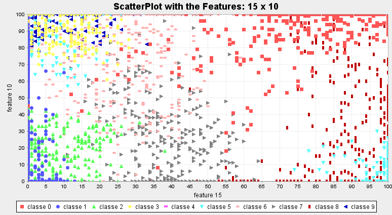
(a) Scatterplot

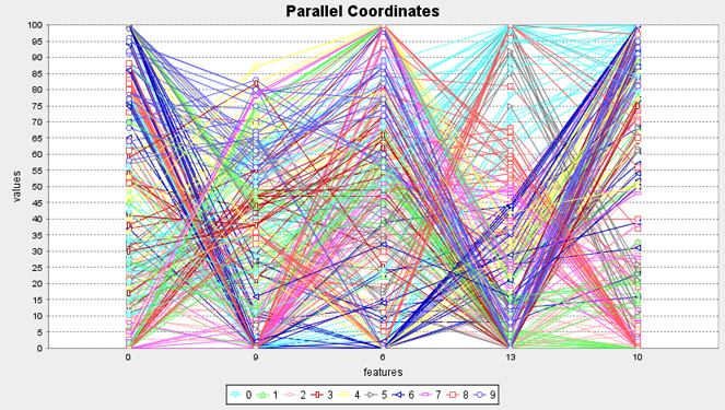
(b) Parallel coordinates

Figure 2: Examples of scatterplot and parallel coordinates generated by the software.

The software is implemented in Java in order to be executable in different platforms. It is open source and intended to be continuously developed in a world-wide collaboration. The software is available at http://code.google.com/p/dimreduction/.

There are four main panels: the first panel allows the user to load the data set (Figure 1-a). The second is optional for the user to define a quantization degree to the data set. The quantized data may be visualized (Figure 1-b). It is worth noting that some feature selection criteria like mean conditional entropy or CoD require data quantization to discrete values. This fact explains the quantization step available in the software. The data quantization is based on a common rule, searching for the extreme values (positive and negative) and dividing equally the negative and positive space considering the number of divisions specified by the quantization degree parameter.

The next step can be the single execution or cross-validation. The first one is dedicated to perform single tests (Figure 1-c). It is represented by a panel where the user is able to enter input parameters such as the feature selection algorithm (see Section 2 for the algorithms implemented) and the criterion function (see Section 3 for the criteria implemented). Other implemented utilities, including the visualization results of the feature selection, area found in the middle of the panel. There are three forms to visualize the results: graphs (Figure 4), scatterplot (Figure 2-a) and parallel coordinates (Figure 2-b). The graphs show the connections among different classes, chosen in feature selection execution, as directed edges between selected vertices. The parallel coordinates proposed by [11] allows to visualize in adjacent axes (selected features) similar patterns of behavior in data, visually indicating how separated are the classes, considering the adjacent features. In the software application, the features and it and its order to build he parallel coordinates chart are defined by the user.

The cross-validation panel (Figure 1-d) is very similar to the prior. Cross-validation [12] consists in to divide the whole data set in two subsets: training and test, mutually exclusive, and the user can define the size of both sets. The training set is entered as input to the feature selection algorithm. The classifier designed from the feature selection and the joint probability distributions table labels the test set samples. At the end of the cross-validation process, it is plotted a chart with the results of each execution, and it is possible to visualize the rate of hits and its variation along the executions.

Another available option is the generalization of non-observed instances. With this option selected, the instances of the selected feature set not present in the training samples are generalized by a nearest neighbors method [1] with Euclidean distance (see Section 3.5 for more details). This method is also applied to take a decision among classes with tied maximum conditional probability distributions given a certain instance.

5 Illustrative Results

This section presents the results in two main aspects. Initially the software was applied as feature selection in a biological classification problem to classify breast cancer cells in two possible classes: benign and malignant. The biological data used here was obtained from [13] which has 589 instances and 32 features. The results shown figure 3, presents very low variations and high accurate classification achieving 99.96% of accuracy on average.

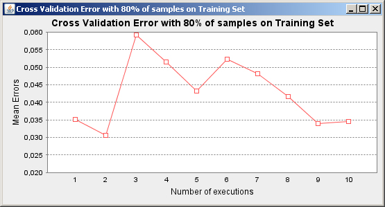
Figure 3: Cross-validation results using 10 executions, 80% of data as training set and 20% as test set.

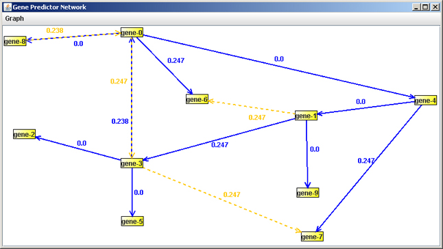
Figure 4: Identified network: dashed lines represent the false positives and solid lines the positives. There are no false negatives.

The second computational biology problem addressed was gene network recovery. In this case we used an artificial gene network generated by the approach presented in [14]. The parameters used were: 10 nodes, binary quantization, 20 observations (timestamps), 1 average of edges per vertex and Random graphs of Erdös-Rényi as network architecture. In figure 4, it is presented the network recovered. This result did not present false negatives and just few false positives.

6 Conclusion

The proposed feature selection environment allows data analysis using several algorithms, criterion functions and graphic visualization tools. Since it is an open-source and multi-platform software, it is suitable for the user that wants to analyze data and draw some conclusions about it, as well as for the specialist that has as objective to compare several combinations of approaches and parameters for each specific data set or to include more features in the software such as a new algorithm or a new criterion function. This system can evolve and include feature extraction methods as well, not limited only to feature selection methods.

The environment can be used in many pattern recognition applications, although the main concern is with Bioinformatics tasks, especially those involving high-dimensional data (large number of genes, for example) with small number of samples. Even users not familiar with programming are allowed to manipulate the software in an easy way, just by clicking to select file inputs, quantization, algorithms, criterion functions, error estimation methods and visualization of the results. The environment is implemented as “wizard style”, i.e., it has tabs delimiting each procedure.

This software opens a great space for future works. The next step consists in the implementation of other classical feature selection algorithms (e.g. GSFS and PTA [1, 15]), criterion functions (e.g. based on distances between classes [1]), error estimation methods (e.g. Leave-one-out and Bootstrap) and then the inclusion of classical methods of feature extraction (e.g. PCA [16]).

References

- [1] S. Theodoridis and K. Koutroumbas. Pattern Recognition. Academic Press, USA, 1st edition, 1999.
- [2] A. K. Jain, R. P. W. Duin, and J. Mao. Statistical pattern recognition: A review. IEEE Transactions on Pattern Analysis and Machine Intelligence, 22(1):4–37, 2000.
- [3] R. O. Duda, P. E. Hart, and D. Stork. Pattern Classification. Wiley-Interscience, NY, 2000.
- [4] T. E. Campos. Técnicas de seleção de características com aplicações em reconhecimento de faces. Master’s thesis, IME-USP, 2001.
- [5] P. Pudil, J. Novovicova, and J. Kittler. Floating search methods in feature-selection. PRL, 15(11):1119–1125, November 1994.
- [6] E. R. Dougherty, S. Kim, and Y. Chen. Coefficient of determination in nonlinear signal processing. Signal Processing, 80:2219–2235, 2000.
- [7] C. E. Shannon. A mathematical theory of communication. Bell System Technical Journal, 27:379–423, 623–656, July, October 1948.
- [8] T. Hsing, L. Liu, Marcel Brun, and E. R. Dougherty. The coefficient of intrinsic dependence (feature selection using el cid). Pattern Recognition, 38(5):623–636, 2005.
- [9] D. C. Martins-Jr, R. M. Cesar-Jr, and J. Barrera. W-operator window design by minimization of mean conditional entropy. Pattern Analysis & Applications, 9:139–153, 2006.
- [10] J. Barrera, R. M. Cesar-Jr, D. C. Martins-Jr, R. Z. N. Vencio, E. F. Merino, M. M. Yamamoto, F. G. Leonardi, C. A. B. Pereira, and H. A. del Portillo. Constructing probabilistic genetic networks of Plasmodium falciparum from dynamical expression signals of the intraerythrocytic development cycle, chapter 2, pages 11–26. Springer, 2006.
- [11] A. Inselberg. The plane with parallel coordinates. The Visual Computer, 1(2):69–91, 1985.
- [12] Ron Kohavi. A study of cross-validation and bootstrap for accuracy estimation and model selection. In IJCAI, pages 1137–1145, 1995.
- [13] A. Asuncion and D.J. Newman. UCI machine learning repository, 2007.
- [14] F. M. Lopes, R. M. Cesar-Jr, and L. F. Costa. Agn simulation and validation model. In Proceedings of Brazilian Symposium on Bioinformatics (in press), 2008.
- [15] P. Somol, P. Pudil, J. Novovicov , and P. Pacl k. Adaptive floating search methods in feature selection. Pattern Recognition Letters, 20:1157–1163, 1999.
- [16] I. T. Jolliffe. Principal component analysis. Springer-Verlag, New York, 1986.