Missing observation analysis for matrix-variate time series data

Abstract

Bayesian inference is developed for matrix-variate dynamic linear models (MV-DLMs), in order to allow missing observation analysis, of any sub-vector or sub-matrix of the observation time series matrix. We propose modifications of the inverted Wishart and matrix $t$ distributions, replacing the scalar degrees of freedom by a diagonal matrix of degrees of freedom. The MV-DLM is then re-defined and modifications of the updating algorithm for missing observations are suggested.

Some key words: Bayesian forecasting, dynamic models, inverted Wishart distribution, state space models.

1 Introduction

Suppose that, in the notation of West and Harrison (1997, Chapter 16), the $p\times r$ matrix-variate time series $\{y_{t}\}$ follows a matrix-variate dynamic linear model (MV-DLM) so that

$$y_{t}^{\prime}=F_{t}^{\prime}\Theta_{t}+\epsilon_{t}^{\prime}\quad\textrm{and}\quad\Theta_{t}=G_{t}\Theta_{t-1}+\omega_{t},$$ (1)

where $F_{t}$ is a $d\times r$ design matrix, $G_{t}$ is a $d\times d$ evolution matrix and $\Theta_{t}$ is a $d\times p$ state matrix. Conditional on a $p\times p$ covariance matrix $\Sigma$, the innovations $\epsilon_{t}$ and $\omega_{t}$ follow, respectively, matrix-variate normal distributions (Dawid, 1981), i.e.

$$\epsilon_{t}|\Sigma\sim N_{r\times p}(0,V_{t},\Sigma)\quad\textrm{and}\quad\omega_{t}|\Sigma\sim N_{d\times p}(0,W_{t},\Sigma).$$

This is equivalent to writing $\textrm{vec}(\epsilon_{t})|\Sigma\sim N_{rp}(0,\Sigma\otimes V_{t})$ and $\textrm{vec}(\omega_{t})|\Sigma\sim N_{dp}(0,\Sigma\otimes W_{t})$, where $\textrm{vec}(.)$ denotes the column stacking operator of a matrix, $\otimes$ denotes the Kronecker product of two matrices and $N_{rp}(.,.)$ denotes the multivariate normal distribution.

We assume that the innovation series $\{\epsilon_{t}\}$ and $\{\omega_{t}\}$ are internally and mutually uncorrelated and also they are uncorrelated with the assumed initial priors

$$\Theta_{0}|\Sigma\sim N_{d\times p}(m_{0},P_{0},\Sigma)\quad\textrm{and}\quad\Sigma\sim IW_{p}(n_{0},n_{0}S_{0}),$$ (2)

for some known $m_{0}$, $P_{0}$, $n_{0}$ and $S_{0}$. Here $\Sigma\sim IW_{p}(n_{0},n_{0}S_{0})$ denotes the inverted Wishart distribution with $n_{0}$ degrees of freedom and parameter matrix $n_{0}S_{0}$. The covariance matrices $V_{t}$ and $W_{t}$ are assumed known; usually $V_{t}=I_{r}$ (the $r\times r$ identity matrix) and $W_{t}$ can be specified using discount factors as in West and Harrison (1997, Chapter 6). Alternatively, $W_{t}=W$ may be considered time-invariant and it can be estimated from the data using the EM algorithm (Dempster et al., 1977; Shumway and Stoffer, 1982). With the above initial priors (2) the posterior distribution of $\Theta_{t}|\Sigma,y_{1},\ldots,y_{t}$ is a matrix-variate normal distribution and the posterior distribution of $\Sigma|y_{1},\ldots,y_{t}$ is an inverted Wishart distribution with degrees of freedom $n_{t}=n_{t-1}+1$ and a parameter matrix $n_{t}S_{t}$, which are calculated recurrently (West and Harrison, 1997, Chapter 16).

Missing data in time series are typically handled by evaluating the likelihood function (Jones, 1980; Ljung, 1982; Shumway and Stoffer, 1982; Harvey and Pierse, 1984; Wincek and Reinsel, 1984; Kohn and Ansley, 1986; Ljung, 1993; Gómez and Maravall, 1994; Luceño, 1994; Luceño, 1997). In the context of model (1) a major obstacle in inference is when a sub-vector or sub-matrix $\widetilde{y}_{t}$ of $y_{t}$ is missing at time $t$. Then the scalar degrees of freedom of the inverted Wishart distribution of $\Sigma|y_{1},\ldots,y_{t}$, are incapable to include the information of the observed part of $y_{t}$, but to exclude the influence of the missing part $\widetilde{y}_{t}$. For example consider $p=2$ and $r=1$ or $y_{t}=[y_{1t}~{}y_{2t}]^{\prime}$ and suppose that at time $t$, $y_{1t}$ is missing ($\widetilde{y}_{t}=y_{1t}$), while $y_{2t}$ is observed. Let $n_{t-1}$ denote the degrees of freedom of the inverted Wishart distribution of $\Sigma|y_{1},\ldots,y_{t-1}$. One question is how one should update $n_{t}$, since the information at time $t$ is partial (one component observed and one missing). Likewise, given this partial information at time $t$, another question is how to estimate the off-diagonal elements of $\Sigma$, which leads to the estimation of the covariance of $y_{1t}$ and $y_{2t}$.

In this paper, introducing several degrees of freedom that form a diagonal matrix, we propose modifications to the inverted Wishart and matrix $t$ distributions. We prove the conjugacy between these distributions and we discuss modifications in the recursions of the posterior moments in the presence of missing data. This approach does not require to order all missing observations in one matrix (Shumway and Stoffer, 1982; Luceño, 1997) and therefore it can be applied for sequential purposes as new data are observed.

2 Matrix-variate dynamic linear models

2.1 Modified inverted Wishart distribution

Suppose that $\Sigma$ is a $p\times p$ random covariance matrix, $S,R$ are $p\times p$ covariance matrices and $N$ is a $p\times p$ diagonal matrix with positive diagonal elements. Let tr$(.)$, etr$(.)$ and $|.|$ denote the trace, the exponent of the trace and the determinant of a square matrix, respectively. The density of the inverted Wishart distribution is given by

$$p(\Sigma)=c|R|^{(k-p-1)/2}|\Sigma|^{-k/2}\textrm{etr}\left(-\frac{1}{2}R\Sigma^{-1}\right),$$ (3)

from which it is deduced that

$$\int_{\Omega}|\Sigma|^{-k/2}\textrm{etr}\left(-\frac{1}{2}R\Sigma^{-1}\right)\,d\Sigma=c^{-1}|R|^{-(k-p-1)/2},$$ (4)

with $\Omega=\{\Sigma\in\mathbb{R}^{p\times p}:\Sigma>0\}$, $c^{-1}=2^{(k-p-1)p/2}\Gamma_{p}\{(k-p-1)/2\}$, and $k>2p$, where $\Gamma_{p}(.)$ is the multivariate gamma function.

Lemma 1.

The function

$$p(\Sigma)=c|\Sigma|^{-\left\{v+\textrm{tr}\left(N\right)/(2p)\right\}}\textrm{etr}\left(-\frac{1}{2}N^{1/2}SN^{1/2}\Sigma^{-1}\right),$$ (5)

where $c$ does not depend on $\Sigma$, is a density function.

Proof.

If the following bijective transformation is applied

$$R=N^{1/2}SN^{1/2}\quad\mbox{and}\quad k=2v+\frac{\textrm{tr}(N)}{p},$$ (6)

then (5) is directly obtained from (3). ∎

From the above bijection and the Wishart integral, we can see that the normalizing constant $c$ is

$$c=c_{0}|S|^{\left\{2v+\textrm{tr}\left(N\right)/p-p-1\right\}/2}\left(\prod_{j=1}^{p}n_{j}\right)^{\left\{2v+\textrm{tr}\left(N\right)/p-p-1\right\}/2},$$

where

$$c_{0}^{-1}=2^{\left\{2v+\textrm{tr}\left(N\right)/p-p-1\right\}p/2}\Gamma_{p}\left\{\frac{2v+\textrm{tr}\left(N\right)/p-p-1}{2}\right\},$$

for $N=\textrm{diag}(n_{1},\ldots,n_{p})$ and $n_{i}>0$ $(i=1,\ldots,p)$.

Density (5) proposes a modification of the inverted Wishart distribution in order to incorporate a diagonal matrix of degrees of freedom. The modification consists of a bijective transform of the two distributions. We will then say that $\Sigma$ follows the modified inverted Wishart distribution and we will write $\Sigma\sim MIW_{p}(S,N,v)$, where $v$ is a scalar hyperparameter. Note that when $n_{1}=\cdots=n_{p}=n$ and $v=p$, the above distribution reduces to an inverted Wishart distribution with $n$ degrees of freedom.

With $k$ and $R$ as defined in equation (6), the mean of $\Sigma$ is

$$E(\Sigma)=\frac{R}{k-2p-2}=\left\{\frac{\textrm{tr}\left(N\right)}{p}+2v-2p-2\right\}^{-1}N^{1/2}SN^{1/2},$$

for $p^{-1}\textrm{tr}(N)>2p-2v+2$. The next result gives the distribution of a $MIW$ matrix conditional on a normal matrix.

Proposition 1.

Let $Y$ be an $r\times p$ random matrix that follows a matrix normal distribution, conditional on $\Sigma$, and $\Sigma$ a $p\times p$ covariance random matrix that follows a modified inverted Wishart distribution, written $Y|\Sigma\sim N_{r\times p}(m,P,\Sigma)$ and $\Sigma\sim MIW_{p}(S,N,v)$ respectively, for some known quantities $m$, $P$, $S$, $N$, and $v$. Then, the conditional distribution of $\Sigma$ given $Y$, is

$$\Sigma|Y\sim MIW_{p}(S^{*},N^{*},v),$$

where $N^{*1/2}S^{*}N^{*1/2}=(Y-m)^{\prime}P^{-1}(Y-m)+N^{1/2}SN^{1/2}$ and $N^{*}=N+rI_{p}$.

Proof.

Form the joint distribution of $Y$ and $\Sigma$ and write

$$p(\Sigma|Y) \propto p(Y,\Sigma)=p(Y|\Sigma)p(\Sigma)$$ (7)

$$\propto |\Sigma|^{-\left\{v+r/2+\textrm{tr}(N)/(2p)\right\}}\textrm{etr}\bigg{[}-\frac{1}{2}\{(Y-f)^{\prime}Q^{-1}(Y-f)$$

$$+N^{1/2}SN^{1/2}\}\Sigma^{-1}\bigg{]},$$

which is sufficient for the proof with the definition of $S^{*}$ and $N^{*}$. ∎

In the context of Proposition 1 the joint distribution of $Y$ and $\Sigma$ is referred to as joint normal modified inverted Wishart distribution with notation $Y,\Sigma\sim NMIW_{r\times p,p}(m,P,S,N,v)$, for $m$, $P$, $S$, $N$, and $v$ as defined in Proposition 1. The next result gives the marginal distribution of $Y$. First we give some background material on the matrix $t$ distribution.

Let $X$ be an $r\times p$ random matrix. Then, the matrix $t$ distribution is defined by

$$p(X)=c|Q+(X-M)^{\prime}P^{-1}(X-M)|^{-(k+r+p-1)/2},$$ (8)

with

$$c=\frac{\Gamma_{p}\{(k+r+p-1)/2\}|Q|^{(k+p-1)/2}|P|^{-p/2}}{\pi^{rp/2}\Gamma_{p}\{(k+p-1)/2\}},$$

where $M$ is an $r\times p$ matrix, $P$ a $r\times r$ covariance matrix, $Q$ a $p\times p$ covariance matrix, and $k$ any positive real number.

Proposition 2.

Let $Y$ be an $r\times p$ random matrix that follows a matrix normal distribution conditional on $\Sigma$, and $\Sigma$ be a $p\times p$ covariance random matrix that follows a modified inverted Wishart distribution, written $Y|\Sigma\sim N_{r\times p}(f,Q,\Sigma)$, and $\Sigma\sim MIW_{p}(S,N,v)$ respectively, for known quantities $f$, $Q$, $S$, $N$, and $v$. Then, the marginal distribution of $Y$ is

$$p(Y)=c|N^{1/2}SN^{1/2}+(Y-f)^{\prime}Q^{-1}(Y-f)|^{-\left\{2v+\textrm{tr}\left(N\right)/p+d-p-1\right\}/2},$$ (9)

which by analogy of the $MIW$ distribution, is a modification of the matrix $t$ distribution and it is written as $MT(f,Q,S,N,v)$.

Proof.

The joint distribution of $Y$ and $\Sigma$ is given by equation (7). Hence, the marginal distribution of $Y$ is

$$p(Y)=\int_{\Omega}p(Y,\Sigma)\,d\Sigma,$$

where $\Omega=\{\Sigma\in\mathbb{R}^{p\times p}:\Sigma>0\}$. Set $R=(Y-f)^{\prime}Q^{-1}(Y-f)+N^{1/2}SN^{1/2}$ and $k=2v+r+\textrm{tr}(N)/p$ and from equation (4) we have equation (9). ∎

The distribution of Proposition (2) can be derived from the matrix $t$ distribution (see equation (8)). The normalizing constant $c$ of (9) is obtainable from (8) as

$$c=\frac{\pi^{pr/2}\Gamma_{p}\{(k+p-1)/2\}}{\Gamma_{p}\{(k+r+p-1)/2\}}|S|^{(k+p-1)/2}\left(\prod_{j=1}^{p}n_{j}\right)^{(k+p-1)/2}|Q|^{-p/2},$$

where $N=\textrm{diag}(n_{1},\ldots,n_{p})$ and $k=2v-2p+\textrm{tr}(N)/p$. Note that if all the diagonal elements of $N$ are the same (i.e. $n_{1}=\cdots=n_{p}=n$) and $v=p$, then the above distribution reduces to a matrix $t$ distribution with $n$ degrees of freedom.

Finally we give the marginal distribution of $\Sigma$. Consider the following partition of $\Sigma$, $S$, and $N$

$$\Sigma=\left[\begin{array}[]{cc}\ \Sigma_{11}&\Sigma_{12}\\ \Sigma_{12}^{\prime}&\Sigma_{22}\end{array}\right],\quad S=\left[\begin{array}[]{cc}\ S_{11}&S_{12}\\ S_{12}^{\prime}&S_{22}\end{array}\right],\quad N=\left[\begin{array}[]{cc}\ N_{1}&0\\ 0^{\prime}&N_{2}\end{array}\right],$$

where $\Sigma_{11}$, $S_{11}$ and $N_{11}$ have dimension $q\times q$, for some $1\leq q<p$. The next result gives the marginal distribution of $\Sigma_{11}$.

Proposition 3.

If $\Sigma\sim MIW_{p}(S,N,v)$, under the above partition of $\Sigma$ the distribution of $\Sigma_{11}$ is $\Sigma_{11}\sim MIW_{q}(S_{11},N_{11},v_{1})$, where $v_{1}=v-p+q+2^{-1}p^{-1}\textrm{tr}(N)-2^{-1}q^{-1}\textrm{tr}(N_{1})$.

Proof.

The proof suggests the adoption of transformation (6) together with the partition of $R$ in (3) as

$$R=\left[\begin{array}[]{cc}R_{11}&R_{12}\\ R_{12}^{\prime}&R_{22}\end{array}\right].$$

Using marginalization properties of the inverted Wishart distribution, upon noticing

$$N^{1/2}SN^{1/2}=\left[\begin{array}[]{cc}\ N_{1}^{1/2}S_{11}N_{1}^{1/2}&N_{1}^{1/2}S_{12}N_{2}^{1/2}\\ N_{2}^{1/2}S_{12}^{\prime}N_{1}^{1/2}&N_{2}^{1/2}S_{22}N_{2}^{1/2}\end{array}\right],$$

we get $\Sigma_{11}\sim MIW_{q}(S_{11},N_{1},v_{1})$, with $v_{1}$ as required. ∎

A similar result can be obtained for $\Sigma_{22}$. Consequently, if we write $\Sigma=\{\sigma_{ij}\}$ $(1\leq i,j\leq p)$ and $N=\textrm{diag}(n_{1},\ldots,n_{p})$, then the diagonal variances $\sigma_{ii}$ follow modified inverted Wishart distributions, $\sigma_{ii}\sim MIW_{1}(s_{ii},n_{i},v_{i})$, where $v_{i}=v-p+1+2^{-1}p^{-1}\textrm{tr}(N)-2^{-1}n_{i}$. These in fact are inverted gamma distributions $\sigma_{ii}\sim IG(v_{i}+n_{i}/2-1,n_{i}s_{ii}/2)$. Note that if $n_{1}=\cdots=n_{p}=n$ and $v=p$, then we have that $\sigma_{ii}\sim IG(n/2,ns_{ii}/2)$ (the inverted gamma distribution used in West and Harrison (1997) when $p=1$).

We close this section with a brief discussion on an earlier study proposing the incorporation of several degrees of freedom for inverted Wishart matrices (Brown et al., 1994). This approach is based on breaking the degrees of freedom on blocks and requiring for each block the marginal density of the covariance matrix to follow an inverted Wishart distribution. However, in that framework the conjugacy between the normal and that distribution is lost and as a result the proposed estimation procedure may be slow and probably not suitable for time series application. Relevant inferential issues of that approach are discussed in Garthwaite and Al-Awadhi (2001). Our proposal of the $MIW$ distribution retains the desired conjugacy and it leads to relevant modifications of the matrix $t$ distribution, which provides the forecast distribution. Furthermore, the $MIW$ density leads to fast computationally efficient algorithms, which are suitable for sequential model monitoring and expert intervention (Salvador and Gargallo, 2004). Finally, according to Proposition 3, the marginal distributions of $MIW$ matrices are also $MIW$, which means that several degrees of freedom are included in the marginal models too, something that is not the case in the approach of Brown et al. (1994).

2.2 Matrix-variate dynamic linear models revisited

We consider model (1), but now we replace the initial priors (2) by the priors

$$\Theta_{0}|\Sigma\sim N_{d\times p}(m_{0},P_{0},\Sigma_{0})\quad\textrm{and}\quad\Sigma_{0}\sim MIW_{p}(S_{0},N_{0},p),$$ (10)

for some known $m_{0}$, $P_{0}$, $S_{0}$ and $N_{0}$. Practically we have replaced the inverted Wishart prior by the $MIW$ and so, for each $t=1,\ldots,T$, we use $p$ degrees of freedom $n_{1t},\ldots,n_{pt}$ in order to estimate $\Sigma|y^{t}$, where $y^{t}$ denotes the information set, comprising of observed data $y_{1},\ldots,y_{t}$. The next result provides the posterior and forecast distributions of the new MV-DLM.

Proposition 4.

One-step forecast and posterior distributions in the model (1) with the initial priors (10), are given, for each $t$, as follows.

(a) Posterior at $t-1:\qquad\Theta_{t-1},\Sigma|y^{t-1}\sim NMIW_{d\times p,p}(m_{t-1},P_{t-1},S_{t-1},N_{t-1},p)$,
for some $m_{t-1}$, $P_{t-1}$, $S_{t-1}$ and $N_{t-1}$.

(b) Prior at $t:\qquad\Theta_{t},\Sigma|y^{t-1}\sim NMIW_{d\times p,p}(a_{t},R_{t},S_{t-1},N_{t-1},p)$,
where $a_{t}=G_{t}m_{t-1}$ and $R_{t}=G_{t}P_{t-1}G_{t}^{\prime}+W_{t}$.

(c) One-step forecast at $t$:$\qquad y_{t}^{\prime}|\Sigma,y^{t-1}\sim N_{r\times p}(f_{t}^{\prime},Q_{t},\Sigma)$,
with marginal:$\qquad y_{t}^{\prime}|y^{t-1}\sim MT_{r\times p}(f_{t}^{\prime},Q_{t},S_{t-1},N_{t-1},p)$,
where $f_{t}^{\prime}=F_{t}^{\prime}a_{t}$ and $Q_{t}=F_{t}^{\prime}R_{t}F_{t}+V_{t}$.

(d) Posterior at $t:\qquad\Theta_{t},\Sigma|y^{t}\sim NMIW_{d\times p,p}(m_{t},P_{t},S_{t},N_{t},p)$,
with

$$m_{t}=a_{t}+A_{t}e_{t}^{\prime},\quad P_{t}=R_{t}-A_{t}Q_{t}A_{t}^{\prime},$$

$$N_{t}=N_{t-1}+rI_{p},\quad N_{t}^{1/2}S_{t}N_{t}^{1/2}=N_{t-1}^{1/2}S_{t-1}N_{t-1}^{1/2}+e_{t}Q_{t}^{-1}e_{t}^{\prime},$$

$$A_{t}=R_{t}F_{t}Q_{t}^{-1},\quad\mbox{and}\quad e_{t}=y_{t}-f_{t}.$$

The proof of this result follows immediately from Propositions 1 and 2. For $t=1$, (a) coincides with the priors (10). From Proposition 2, the marginal posterior of $\Theta_{t}|y^{t}$ is $\Theta_{t}|y^{t}\sim MT_{d\times p}(m_{t},P_{t},S_{t},N_{t},p)$. Thus the above proposition gives a recursive algorithm for the estimation and forecasting of the system for all $t=1,\ldots,T$.

Proposition 4 gives a generalization of the updating recursions of matrix-variate dynamic models (West and Harrison, 1997, Chapter 16). The main difference of the two algorithms is that the scalar degrees of freedom $n_{t}$ of the standard recursions are replaced by $N_{t}$ in the above proposition and that the inverted Wishart distribution is replaced by the modified inverted Wishart distribution (in order to account for the matrix of degrees of freedom). As a result the classical Bayesian updating of West and Harrison (1997) is obtained as a special case of the distributional results of Proposition 4, by setting $N_{t}=n_{t}I_{p}=\textrm{diag}(n_{t},\ldots,n_{t})$ $(t=0,1,\ldots,T)$, where $n_{t}$ represent the scalar degrees of freedom of the inverted Wishart distribution of $\Sigma_{t}|y^{t}$ and $n_{0}$ is the initial degrees of freedom.

3 Missing observations

In this section we consider missing observations at random. Our approach is based on excluding any missing values of the calculation of the updating equations (state and forecast distributions) thus excluding the unknown influence of these unobserved variables. This approach is explained for univariate dynamic models in West and Harrison (1997, Chapters 4,10).

The univariate dynamic linear model with unknown observational variance is obtained from model (1) for $p=r=1$. In this case the posterior recursions of $m_{t}$, $P_{t}$ and $S_{t}$ of West and Harrison (1997, Chapter 4) follow from Proposition 4 as a special case. Now suppose that at time $t$ the scalar observation $y_{t}$ is missing so that $y^{t}=y^{t-1}$. It is then obvious that the posterior distribution of $\Theta_{t}$ equals its prior distribution (since no information comes in to the system at time $t$). Then we have $m_{t}=a_{t}$, $P_{t}=R_{t}$, $S_{t}=S_{t-1}$ and $N_{t}=n_{t}=n_{t-1}=N_{t-1}$. To incorporate this into the updating equations of the posterior means and variances, we can write $m_{t}=a_{t}-A_{t}e_{t}u_{t}$, $P_{t}=R_{t}-A_{t}A_{t}^{\prime}Q_{t}u_{t}$, $n_{t}S_{t}=n_{t-1}S_{t-1}+e_{t}^{2}u_{t}/Q_{t}$ and $n_{t}=n_{t-1}+u_{t}$, where $u_{t}$ is zero, if $y_{t}$ is missing and $u_{t}=1$, if $y_{t}$ is observed. So when $p=1$ the inclusion of $u_{t}$ in the posterior recursions leads to identical analysis as in West and Harrison (1997) and in references therein. The introduction of $u_{t}$ in the recursions automates the posterior/prior updating in the presence of missing values and it motivates the case for $p,r\geq 1$.

Moving to the multivariate case, first we consider model (1) as defined in the previous section with $r=1$. Assume that we observe all the $p\times 1$ vectors $y_{i}$, $i=1,\ldots,t-1$. At time $t$ some observations are missing (sub-vectors of $y_{t}$, or the entire $y_{t}$). To distinguish the former from the latter case we have the following definition.

Definition 1.

A partial missing observation vector is said to be any strictly sub-vector of the observation vector that is missing. If the entire observation vector is missing it is referred to as full missing observation vector.

Considering the MV-DLM (1), it is clear that in the case of a full missing vector we have

$$\Theta_{t},\Sigma|y^{t}\sim NMIW_{d\times p,p}(m_{t},P_{t},S_{t},N_{t},p),$$ (11)

where $m_{t}=a_{t}$, $P_{t}=R_{t}$, $S_{t}=S_{t-1}$, $N_{t}=N_{t-1}$, since no information comes in at time $t$. This equation relates to the standard posterior distribution of West and Harrison (1997) by setting $N_{t}=\textrm{diag}(n_{t},\ldots,n_{t})$, for a scalar $n_{t}>0$ and evidently reducing the $MIW$ distribution by a $IW$ distribution. If one starts with a prior $N_{0}=\textrm{diag}(n_{0},\ldots,n_{0})$, and assuming that at some time $t$, there is a full missing vector $y_{t}$, then it is clear that the posterior (11) equals to the posterior of $\Theta_{t},\Sigma|y^{t}$ using the standard recursions (West and Harrison, 1997). Any differences between the two algorithms is highlighted only by observing partial missing vectors and this has been the motivation of the new algorithm.

Define a $p\times p$ diagonal matrix $U_{t}=\mbox{diag}(i_{1t},\ldots,i_{pt})$ with

$$i_{jt}=\left\{\begin{array}[]{cc}1&\textrm{if $y_{jt}$ is observed},\\ 0&\textrm{if $y_{jt}$ is missing,}\end{array}\right.$$

for all $1\leq j\leq p$, where $y_{t}=[y_{1t}~{}\cdots~{}y_{pt}]^{\prime}$.

Then, the posterior distribution (11) still applies with recurrences

$$m_{t}=a_{t}+A_{t}e_{t}^{\prime}U_{t}$$ (12)

$$P_{t}=R_{t}-A_{t}A_{t}^{\prime}Q_{t}u_{t}$$ (13)

$$N_{t}=N_{t-1}+U_{t}$$ (14)

$$N_{t}^{1/2}S_{t}N_{t}^{1/2}=N_{t-1}^{1/2}S_{t-1}N_{t-1}^{1/2}+U_{t}e_{t}Q_{t}^{-1}e_{t}^{\prime}U_{t},$$ (15)

where $u_{t}=\mbox{tr}(U_{t})/p$. Some explanation for the above formulae are in order.

First note that if no missing observation occurs $U_{t}=I_{p}$, $u_{t}=1$ and we have the standard recurrences as in Proposition 4. On the other extreme (full missing vector), $U_{t}=0$, $u_{t}=0$ and we have equation (11). Consider now the case of partial missing observations. Equation (14) is the natural extension of the single degrees of freedom updating, see West and Harrison (1997, Chapter 16). For equation (12) note that the zero’s of the main diagonal of $U_{t}$ convey the idea that the corresponding to the missing values elements of $m_{t}$ remain unchanged and equal to $a_{t}$. For example, consider the case of $p=2$, $d=2$ and assume that you observe $y_{1t}$, but $y_{2t}$ is missing. Then

$$m_{t}=a_{t}+\left[\begin{array}[]{cc}\ A_{1t}(y_{1t}-f_{1t})&0\\ A_{2t}(y_{1t}-f_{1t})&0\end{array}\right],$$

where $A_{t}=[A_{1t}~{}A_{2t}]^{\prime}$. The zero’s on the right hand side reveal that the second column of $m_{t}$ is the same as the second column of $a_{t}$. Similar comments apply for equations (13) and (15).

Considering the case of $r\geq 2$, we define $U_{kt}$ to be the diagonal matrix $U_{kt}=\mbox{diag}(i_{1k,t},\ldots,i_{pk,t})$ with

$$i_{jk,t}=\left\{\begin{array}[]{cc}1&\textrm{if $y_{jk,t}$ is observed},\\ 0&\textrm{if $y_{jk,t}$ is missing,}\end{array}\right.$$

where $y_{t}=\{y_{jk,t}\}$, $(j=1,\ldots,p;k=1,\ldots,r)$.

Then, the moments of equation (11) can be updated via

$$m_{t}=a_{t}+A_{t}e_{t}^{\prime}\prod_{k=1}^{r}U_{kt},\quad P_{t}=R_{t}-A_{t}Q_{t}A_{t}^{\prime}u_{t},\quad N_{t}=N_{t-1}+\sum_{k=1}^{r}U_{kt}$$

$$N_{t}^{1/2}S_{t}N_{t}^{1/2}=N_{t-1}^{1/2}S_{t-1}N_{t-1}^{1/2}+\left(\prod_{k=1}^{r}U_{kt}\right)e_{t}Q_{t}^{-1}e_{t}^{\prime}\left(\prod_{k=1}^{r}U_{kt}\right),$$

where $u_{t}=\mbox{tr}(\prod_{k=1}^{r}U_{kt})/p$. Similar comments as in the case of $r=1$ apply. Definition 1 is trivially extended in the case when observations form a matrix ($r\geq 2$).

We illustrate the proposed methodology by considering simulated data, consisting of 100 bivariate time series $y_{1},\ldots,y_{100}$, generated from a local level model $y_{t}=[y_{1t}~{}y_{2t}]^{\prime}=\psi_{t}+\epsilon_{t}$ and $\psi_{t}=\psi_{t-1}+\zeta_{t}$, where $\psi_{0}$, $\epsilon_{t}$ and $\zeta_{t}$ are all simulated from bivariate normal distributions. The correlation of $\epsilon_{1t}$ and $\epsilon_{2t}$ is set to $0.8$, while the elements of $\zeta_{t}$ are uncorrelated. This model is a special case of model (1) with $\Theta_{t}^{\prime}F_{t}=\psi_{t}$ and $G_{t}=I_{2}$. Figure 1 (solid line) shows the simulated data; the gaps in this figure indicate missing values at times $t=24,43,60,75,86$. At times $t=24,43,86$, $y_{t2}$ is only missing (partial missing vectors), at time $t=75$, $y_{t1}$ is only missing (partial missing vector) and at time $t=60$, both $y_{t1},y_{t2}$ are missing (full missing vector). For this data set, we compare the performance of recursions (12)-(15) with that of the classic or old recursions of West and Harrison (1997), which assume that when there is at least one missing value we set $U_{t}=0$ and $u_{t}=0$. For example using the old recursions, for $t=24$ one would set $U_{24}=0$ and $u_{24}=0$, losing the “partial” information of $y_{24,1}=-3.739$, which is observed. On the other hand, the new recursions would suggest for $t=24$ to set

$$U_{24}=\left[\begin{array}[]{cc}1&0\\ 0&0\end{array}\right]\quad\textrm{and}\quad u_{24}=1/2.$$

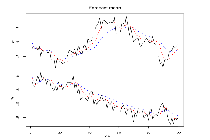
Figure 1: Simulated bivariate time series (solid line) with one-step forecasts from (a) the standard DLM recursions (dotted/dashed line) and (b) the new DLM recursions (dashed line). The gaps indicate missing values.

Figure 1 shows the one-step forecast mean of $\{y_{t}\}$ using the new recursions (dashed line) and the old recursions (dotted/dashed line). We observe that the new method produces a clear improvement in the forecasts as the old recursions provide poor forecasts, especially in the low panel of Figure 1 (for $\{y_{1t}\}$). What is really happening in this case is that, under the old recursions, the missing values of $y_{2t}$ affect the recursions for $y_{1t}$, since the observed information at $y_{1t}$ is wrongly “masked” or “ignored” for the points of time when $y_{2t}$ is missing. On the other hand, the new recursions use the explicit information from each sub-vector of $y_{t}$ and thus the new recursions result in a notably more accurate forecast performance. This is backed by the mean square standardized forecast error vector, which for the new recursions is $[1.300~{}1.825]^{\prime}$, while for the old recursions is $[1.545~{}2.182]^{\prime}$. Under the old recursions we can not obtain an estimate of the covariance between an observed $y_{1t}$ and a missing $y_{2t}$. However, this is indeed obtained under the proposed new recursions and so the respective correlations at points of time where there are gaps are $0.633$ (at $t=24$), $0.779$ (at $t=43$), $0.812$ (at $t=75$) and $0.809$ (at $t=86$); the mean of these correlations is $0.792$, which is close to the real $0.8$ under the simulation experiment.

References

• [1] Brown, P.J., Le, N.D. and Zidek, J.V. (1994) Inference for a covariance matrix. In Aspects of Uncertainty (eds P.R. Freeman, A.F.M. Smith). Chichester: Wiley.
• [2] Dawid, A.P. (1981), Some matrix-variate distribution theory: notational considerations and a Bayesian application, Biometrika, 68, 265-274.
• [3] Dempster, A.P., Laird, N.M. and Rubin, D.B. (1977) Maximum likelihood from incomplete data via the EM algorithm (with discussion). Journal of the Royal Statistical Society Series B, 39, 1-38.
• [4] Garthwaite, P.H. and Al-Awadhi, S.A. (2001) Non-conjugate prior distribution assessment for multivariate normal sampling. Journal of the Royal Statistical Society Series B, 63, 95-110.
• [5] GΓ³mez, V. and Marvall, D. (1994) Estimation, prediction, and interpolation for nonstationary series with the Kalman filter. Journal of the American Statistical Association, 89, 611-624.
• [6] Harvey, A.C. and Pierse, R.G. (1984) Estimating missing observations in economic time series. Journal of the American Statistical Association, 79, 125-131.
• [7] Jones, R.H. (1980) Maximum likelihood fitting of ARMA models to time series with missing observations. Technometrics, 22, 125-131.
• [8] Kohn, R. and Ansley, C.F. (1986) Estimation, prediction, and interpolation for ARIMA models with missing observations. Journal of the American Statistical Association, 81, 751-761.
• [9] Ljung, G.M. (1982) The likelihood function of a stationary Gaussian autoregressive-moving-average process with missing observations. Biometrika, 69, 265-268.
• [10] Ljung, G.M. (1993) On outlier detection in time series. Journal of the Royal Statistical Society B, 55, 559-567.
• [11] LuceΓ±o, A. (1994) A fast algorithm for the exact likelihood of stationary and partially nonstationary vector autoregressive moving average processes. Biometrika, 81, 555-565.
• [12] LuceΓ±o, A. (1997) Estimation of missing values in possibly partially nonstationary vector time series. Biometrika, 84, 495-499.
• [13] Salvador, M. and Gargallo, P. (2004). Automatic monitoring and intervention in multivariate dynamic linear models. Computational Statistics and Data Analysis, 47, 401-431.
• [14] Shumway, R.H. and Stoffer, D.S. (1982) An approach to time series smoothing and forecasting using the EM algorithm. Journal of Time Series Analysis, 3, 253-264.
• [15] West, M. and Harrison, P.J. (1997) Bayesian Forecasting and Dynamic Models, Springer-Verlag (second edition), New York.
• [16] Wincek, M.A. and Reinsel, G.C. (1986) An exact maximum likelihood estimation procedure for regression-ARMA time series models with possibly nonconsecutive data. Journal of the Royal Statistical Society B, 48, 303-313.