Many-Body meets QM/MM: Application to indole in water solution

Abstract

Spectral properties of chromophores are used to probe complex biological processes in vitro and in vivo, yet how the environment tunes their optical properties is far from being fully understood. Here we present a method to calculate such properties on large scale systems, like biologically relevant molecules in aqueous solution. Our approach is based on many body perturbation theory combined with quantum-mechanics/molecular-mechanics (QM/MM) approach. We show here how to include quasi-particle and excitonic effects for the calculation of optical absorption spectra in a QM/MM scheme. We apply this scheme, together with the well established TDDFT approach, to indole in water solution. Our calculations show that the solvent induces a redshift in the main spectral peak of indole, in quantitative agreement with the experiments and point to the importance of performing averages over molecular dynamics configurations for calculating optical properties.

Optical properties of aromatic chromophores embody a key facet of cell biology, allowing for a precise interrogation of a variety of biochemical events, including signaling, metabolism and aberrant processes. These range from probing transient interactions between biomolecules (proteins and nucleic acids), to protein dynamics and fibrillation and plaque formation in neurodegenerative diseases. Understanding how the environment tunes such optical properties is therefore crucial in structural genomics, yet this information is so far mostly lacking. A powerful tool to address this issue is given by the so-called quantum-mechanics/molecular-mechanics (QM/MM) methods [qmmm1, ; qmmm2, ; qmmm3, ; qmmm4, ; qmmm5, ; qmmm6, ; qmmm7, ]. In this approach, the aromatic moiety is treated at quantum mechanical level, whilst the environment is described with an effective potential: the influence of the MM (presumably very complex and very large) environment is basically included as an external potential, and, in case the molecule is covalently bound to MM region, by a mechanical coupling with the environment.

Most often the QM approach is solved within Density Functional Theory (DFT) [dft1, ; dft2, ] to study ground state properties, and time-dependent DFT (TDDFT) [tddft1, ; tddft2, ] when excited states are involved as in the case of the optical properties [tddftmm1, ; tddftmm2, ; tddftmm3, ]. TDDFT is computationally very efficient, yet its predictive power depends dramatically on the system and on the functional used to reproduce the exchange and correlation interactions.

Several approaches, including Post-Hartree-Fock ones [Olivucci, ] (configuration interaction and similar methods), have been already used to predict optical properties of biomolecules. Quantum-many-body techniques (MBPT) [gw1, ; bse, ], are an attractive alternative, although of course they come with a much higher computational cost than TDDFT. Strikingly, however, biophysical applications of one of the most widely used scheme, the combination of the GW method [gw1, ] with the Bethe-Salpeter Equation (BSE) [bse, ] are so far lacking. The GW method is used for the evaluation of the single quasiparticle energies, and the BSE to introduce excitonic effects. Keeping in mind future biological applications, it is imperative to assess the accuracy of a MBPT/MM approach versus the more conventional TDDFT/MM one.

The main assumption in interfacing a QM/MM method with TDDFT or MBPT approaches is that the optical properties of the chromophore do not involve the MM part’s electronic structure. Hence, special care has to be devoted to the choice of the two regions.

Here we present MBPT/MM calculations on the indole ring of the Tryptophan protein residue (Fig. 1). This system appears ideal for such an approach in several respects. First, it is very relevant biologically, as the indole ring has been exploited as a spectroscopic tool to monitor changes in proteins [Creed, ] and to yield information about local structure and dynamics. In fact, its spectral signatures allow it to be used as a structural probe in proteins. Second, it contains a relatively small number of atoms (16), which can still be treated at the GW-BSE level. Next, the optical gap of liquid water (7 eV [exp-water1, ; exp-water2, ; viviana, ]) is larger than the gap of the indole molecule (4.3 eV [exp_indole2, ]). Under 7 eV the spectra of indole and water do not overlap, and it is justified to treat the solvent in a classical scheme. Finally, CASPT2 calculations [exp_indole2, ] and experimental data [exp_indole1, ] are available, and allow to compare the changes of the optical properties upon passing from the gas phase to aqueous solution.

We performed QM/MM Car-Parrinello [carparrinello, ] simulations of indole in water by the fully Hamiltonian QM/MM scheme [qmmm7, ]. Such scheme has been applied to a variety of biological systems [dalperaro, ]. The biomolecule was treated, at this step, at the DFT level whilst the solvent with the Amber force field [amber, ]. The approach allows for an explicit treatment of solvation, in contrast to previous studies [exp_indole1, ; exp_indole2, ; exp_indole3, ].

Indole single quasiparticle energies have been then evaluated at the GW level for several snapshots. Finally, we solved the BSE to calculate the average absorption spectrum and compared the results with the ones obtained within TDDFT. We calculated the indole absorbance in water as well as in gas phase. The shift in the spectra gives the solvatochromism.

The GW approximation consists in setting the vertex in the Hedin equations [hedin, ] equal to a delta function. Under this condition, the time-Fourier transform of the proper exchange-correlation self energy, $\Sigma(\mathbf{{r},{r^{\prime}},\omega)}$, is a convolution of the Green function $G(\mathbf{{r},{r^{\prime}},\omega)}$, with the screened Coulomb potential $W(\mathbf{{r},{r^{\prime}},\omega)}$. The electronic bands are obtained by solving the following eigenproblem:

$$\left[-\frac{\hbar^{2}\nabla^{2}}{2m}+U^{QM}(\mathbf{r})+U^{QM/MM}(\mathbf{r})+V_{H}(\mathbf{r})\right]\phi_{j}(\mathbf{r}) +$$

$$\int d^{3}\mathbf{{r^{\prime}}}\Sigma(\mathbf{{r},{r^{\prime}}},\varepsilon^{QP}_{j})\phi_{j}(\mathbf{r^{\prime}})=\varepsilon^{QP}_{j}\phi_{j}({\mathbf{r}}).$$ (1)

This expression is derived from the Dyson equation in Lehmann representation [gw1, ]. $V_{H}$ is the Hartree potential of the QM part, $U^{QM}$ is the electron-ion potential of the QM part, while $U^{QM/MM}$ is the potential felt by the electrons due to the point charges of the MM part. Finally, $\varepsilon_{j}^{QP}$ are the quasi-particle eigenvalues. Eq. (1) has the same form as the KS equation [dft2, ] in the presence of an external electric field, where the exchange-correlation potential $V_{xc}(\mathbf{r}$) is replaced by the self energy $\Sigma(\mathbf{{r},{r^{\prime}}},\varepsilon_{j}^{QP})$ which acts as a non-local, energy-dependent potential. Therefore, the eigenvalue problem described above can be solved perturbatively considering the KS equation as an unperturbed Hamiltonian and $\Sigma-V_{xc}$ as a perturbative term. The quasi-particle eigenvalues are obtained in first order approximation:

$$\varepsilon^{QP}_{j}=\varepsilon^{KS}_{j}+\frac{\langle\phi_{j}^{KS}|\Sigma(\varepsilon_{j}^{KS})-V_{xc}|\phi_{j}^{KS}\rangle}{1-\langle\phi_{j}^{KS}|\frac{d\Sigma(\varepsilon^{KS}_{j})}{d\omega}|\phi_{j}^{KS}\rangle}.$$ (2)

All the Coulomb interactions, and hence also the one induced by the classical region, are included in the KS eigenvalues $\varepsilon^{KS}_{j}$, and eigenvectors $|\phi_{j}^{KS}\rangle$. In this GW/MM scheme we neglect the contribution of the classical atoms to the $\Sigma$ operator in the same way as it is neglected for $V_{xc}$ in the DFT/MM scheme.

As a bonus from GW calculations we obtain also the four-point independent quasi-particle polarizability required to solve the BSE and which reads, in transition space [bse, ]:

$$P^{0}_{(n1,n2)(n3,n4)}(\omega)=\frac{f_{n2}-f_{n1}}{\varepsilon^{QP}_{n2}-\varepsilon^{QP}_{n1}-\omega}\delta_{n1,n3}\delta_{n2,n4}$$ (3)

where $f_{n}$ is the occupation numbers of level $n$: the quantum plus classical external potential is not explicitly present in the BSE, but indirectly determines all the ingredients.

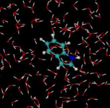
Figure 1: (color online) Indole in water solution. Colors correspond to the following atomic species: BLUE=N, CYAN=C, WHITE=H, RED=O.

We performed a 20 ps hybrid QM/MM Car-Parrinello simulation of an indole molecule (QM part) [detailsDynamics, ] surrounded by 2000 water molecules treated classically (MM part), with the Amber force field [detailsMM, ]. Such a large number of water molecules was necessary to correctly reproduce the physical properties of a disordered system such as liquid water at room temperature (300 K). We also verified that such a large number of water molecules used for the dynamics was also necessary to calculate the optical absorption spectrum. This became clear already at the DFT-independent particle approach (DFT-IPA), as shown in Fig.2: we calculated the absorption spectrum for indole with no water (with indole in the same ”distorted” geometrical configuration as if in water), for indole with 2 water molecules, and for indole with 2000 water molecules. The three spectra are all different. This is a strong indication that also for the absorption spectrum it is necessary to include many water molecules in the theoretical simulation. This is due to the long range electrostatic potential of water which acts on indole.

Next, we tested our assumption that the solvent can be treated classically in the calculation of absorption spectra by performing TDDFT calculations [detailsTDDFT, ] for a system where two water molecules were treated at quantum level, and the remaining 1998 classically. The position of absorption peak is the same (within 0.02 eV) as in the case where all waters were treated within MM. Our result supports the use of this approach for solutes in water [tddftmm2, ].

For ten snapshots of the QM/MM dynamics (one every two ps) we computed the optical spectra at the independent particle level (DFT-IPA) and within TDDFT. The final spectrum was obtained by an average over the snapshots. The convergence of the spectrum was reached already after 6 snapshots, hence the subsequent GW and BSE calculations have been performed on only 6 snapshots.

The calculated DFT and GW HOMO-LUMO gaps [detailsGW, ], averaged over the QM/MM configurations, are 3.8 eV (with standard deviation $\sigma=\pm$ 0.1 eV) and 7.2($\sigma=\pm$ 0.2) eV, respectively. The GW corrections to the gap turned out to be practically constant in all the snapshots considered (3.4 $\pm$ 0.1 eV). This fact, already found for liquid water [viviana, ], confirms that one can strongly reduce the computational effort, by performing a GW calculations for just one snapshot.

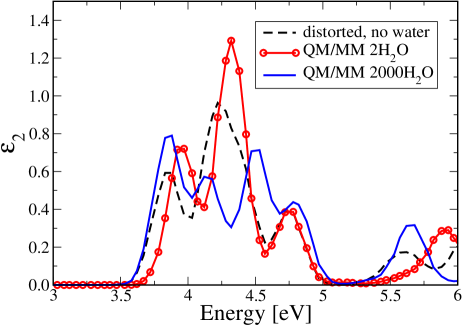
Figure 2: (color online) DFT-IPA optical spectra of indole in 2000 water molecules (blue solid line), in 2 water molecules (red circles) and without water (black dashed line).

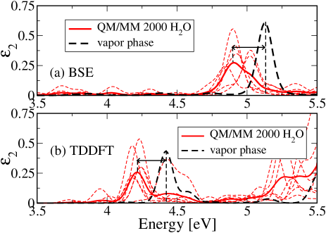
Figure 3: (color online) BSE (a) and TDDFT (b) spectra of indole in water. The tiny red dashed lines are the spectrum of each snapshot. The red solid line is obtained by an average over these spectra. The black dashed line is for indole in vapor phase.

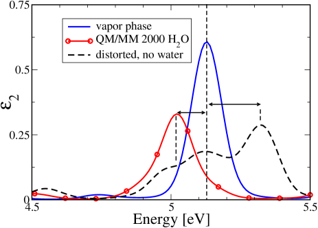
Figure 4: (color online) BSE optical spectra. Solid blue line: Indole in vapor phase. Black dashed line: indole without water molecules, with distorted geometry taken from a snapshot corresponding to 13.08 ps of the dynamics. Circles: indole in water, spectrum calculated for the same snapshot.

We finally calculate the low energy range of the optical spectrum of indole, by GW-BSE and TDDFT, always as result of an average over the QM/MM snapshots. In Fig.3 we report our results together with the calculated absorption spectrum in gas phase. We notice that, in both approaches the most intense peak (${}^{1}L_{a}$ in the experiment) is red-shifted on passing from gas phase to the water solution. This agrees with experiments [exp_indole1, ]. Same conclusion was obtained by previous theoretical calculations of indole in water based on CASSCF method and CASPT2 [exp_indole2, ]. In these approaches, the solvent was simulated by a continuum model with a cavity containing the indole molecule. The value we calculate for such a redshift is $\sim$ 0.2 eV, in fair agreement with experiment (0.18 eV) [exp_indole1, ]. On the contrary the CASSCF and CASPT2 prediction for the solvent shift is about 0.06 eV only. Such an underestimation may depend on the geometrical distortion of indole molecule caused by temperature effects due to the solvent and by an explicit H-bonding between water molecules, which were not considered explicitly therein. To quantify the effect of the geometry distortion on such shift, we performed calculations of indole switching on and off the water field in order to separate the geometry effect from the electrostatic ones. The results are presented for a single snapshot in GW+BSE (Fig. 4) and are obtained by performing additional calculations for the same QM/MM configuration without the water field. The corresponding solvent-shift goes from -0.1 eV with water field to +0.2 eV (hence, a blue-shift) without water field. This emphasises the importance of taking into account explicitly the electrostatic interaction with the solvent, since the geometry distortion alone would give, at least for this snapshot, a wrong sign.

In addition, TDDFT underestimates the energy of the ${}^{1}L_{a}$ peak both in gas phase and in solution by $\sim$0.4 eV, and BSE-GW overestimates them by $\sim$0.3 eV. As expected [exp_indole3, ], CASSCF is much worse, it overestimates by $\sim$1 eV or more, whilst CASPT2 is more accurate ($\sim$0.13 eV or less).

In conclusion, we have included many-body perturbative techniques in a QM/MM scheme. We have applied it, together with a TDDFT/MM approach, to study the optical properties of indole in water solution. Both methods reproduce quantitatively the redshift induced by the solvent. Hence, the GW-BSE method could be applied to biomolecules in aqueous solution (i.e. in laboratory-realizable conditions) in cases where the TDLDA/GGA approach does not work [failure1, ; failure2, ]. Our GW-BSE calculations further show that the solvent shift is a consequence of the combination of two effects: the geometrical distortion of indole molecule in the solvent and the electrostatic interaction with the water molecules electric dipoles. Both effects, and their sum, depend on the particular configuration of the system; this emphasizes the need of more than one snapshot (several, indeed) for carrying out accurate optical calculations.

This work opens the way to further applications in other bio-relevant molecules, such as proteins and cell membranes, for which the evaluation of the optical shift enables to understand the nature of their environment.

This work was supported by the EU through the Nanoquanta NOE (NMP4-CT-2004-500198). Computer resources from INFM “Progetto Calcolo Parallelo” at CINECA are gratefully acknowledged. We also thank L. Guidoni for interesting discussions.

References

- (1) E. A. Carter , and J. T. Hynes, J. Chem. Phys. 94, 5961 (1991).
- (2) M. Maroncelli, J. Chem. Phys. 94, 2084 (1991).
- (3) P. V. Kumar, and M. Maroncelli, J. Chem. Phys. 103, 3038 (1995).
- (4) F. Chichos, R. Brown, U. Rempel, and C. von Borczyskowski, J. Phys. Chem. A 103, 2506 (1999).
- (5) F. Chichos, R. Brown, and Ph. A. Bopp, J. Chem. Phys. 114, 6824 (2001).
- (6) F. Chichos, R. Brown, and Ph. A. Bopp, J. Chem. Phys. 114, 6834 (2001).
- (7) A. Laio, J. VandeVondele, and U. Rthlisberger, J. Chem. Phys. 116, 6941 (2002).
- (8) P. Hohenberg, and W. Kohn, Phys. Rev. 136 B864 (1964).
- (9) W. Kohn, and L. J. Sham, Phys. Rev. 140 A1133 (1965).
- (10) E. Runge, and E. K. U. Gross, Phys. Rev. Lett. 52, 997 (1984).
- (11) Miguel A. L. Marques, and Eberhard K. U. Gross, Time-Dependent Density Functional Theory, Springer-Verlag Berlin Heidelberg (2003).
- (12) M. Sulpizi, P. Carloni, J. Hutter, and U. Rthlisberger, Phys. Chem. Chem. Phys 5, 4798 (2003).
- (13) M. Sulpizi, U. F. Rhrig, J. Hutter, and U. Rthlisberger, Int. J. Quantum Chem. 101, 671 (2004).
- (14) M-E. Moret, E. Tapavicza, L. Guidoni, U. F. Rhrig, M. Sulpizi, I. Tavernelli, and U. Rthlisberger, CHIMIA International Journal for Chemistry 59, 493-498 (2005).
- (15) L. M. Frutos, T. Andruniów, F. Santoro, N. Ferré, and M. Olivucci, Proc. Nat. Acad. Sci. 104, 7764 (2007).
- (16) see for example Quantum theory of many-particle systems, A.L. Fetter, J.D. Walecka ,McGraw-Hill, San Francisco (1971).
- (17) G Onida, L Reining, A Rubio, Rev. Mod. Phys. 74 601 (2002).
- (18) D. Creed, Photochem. Photobiol, 39, 537 (1984).
- (19) G. D. Kerr, R. N. Hamm, M. W. Williams, R. D. Birkhoff, and L. R. Painter, Phys. Rev. A 5 2523 (1972).
- (20) L. R. Painter, R. N. Hamm, E. T. Arakawa, and R. D. Birkhoff, Phys. Rev. Lett. 21 282 (1968).
- (21) V. Garbuio, M. Cascella, L. Reining, R. Del Sole, and O. Pulci, Phys. Rev. Lett. 97 137402 (2006).
- (22) L. Serrano-Andres, and B. O. Roos, J. Am. Chem. Soc. 118 185 (1996) and references therein.
- (23) H. Lami, J. Chem. Phys. 67 3274 (1977).
- (24) R. Car, and M. Parrinello, Phys. Rev. Lett. 55 2471 (1985).
- (25) M. Dal Peraro, P. Ruggerone, S. Raugei, F. L. Gervasio, P. Carloni, Curr. Opin. Struct. Biol. 17(2), 149 (2007).
- (26) D. A. Pearlman, D. A. Case, J. W. Caldwell, W. S. Ross, T. E. Cheatham, S. Debolt, D. Ferguson, G. Seibel, P. Kollman, Comput. Phys. Commun. 91, 1 (1995).
- (27) D. M. Rogers, and J. D. Hirst, J. Phys. Chem. 107 11191 (2003).
- (28) L. Hedin, Phys. Rev. 139 A796 (1965).
- (29) The QM/MM code combines the CPMD3.11.1 [cpmd, ] and Gromos [gromos, ] codes. The time step chosen for the simulations was about 0.1 fs. Since the indole’s N–H group forms H-bonds with water, we used an energy cutoff of 70 Ry with the BLYP recipe [blyp, ] for the exchange-correlation functional, which have widely been used for biophysical applications. Norm-conserving pseudopotentials of Troullier-Martins type [TM, ] corrected for a better description of Van der Walls interactions [VdW, ] have been used. A Nose-Hoover thermostat [nose, ; nose1, ] is applied throughout all simulations to keep the temperature constant.
- (30) J. Hutter, A. Alavi, T. Deutsch, P. Ballone, M. Bernasconi, P. Focher, S. Goedecker, M. Tuckerman, M Parrinello, CPMD, Copyright IBM Corp 1990-2006, Copyright MPI für Festkörperforschung, Stuttgart 1997-2001.
- (31) W. F. van Gunsteren, S. R. Billeter, A. A. Eising, P. H. Hünenberger, P. Krüger, A. E. Mark, W. R. P. Scott, I. G. Tironi, Biomolecular Simulation: The GROMOS96 Manual and User Guide; Vdf Hochschulverlag AG an der ETH Zürich: Zürich, 1996.
- (32) A. D. Becke, Phys. Rev. A 38, 3098 (1988); C. Lee, W. Yang, and R. G. Parr, Phys. Rev. B 37, 785 (1988).
- (33) N. Troullier and J. L. Martins, Phys. Rev. B 43, 1993 (1991).
- (34) O. A. von Lilienfeld, I. Tavernelli, U. Rthlisberger, and D. Sebastiani, Phys. Rev. Lett. 93, 153004 (2004).
- (35) S. J. Nosé, J. Chem. Phys. 81, 511 (1984).
- (36) D. J. Evans and B. L. Holian, J. Chem. Phys. 83, 4069 (1985).
- (37) We used the Parm99 version of Amber force field with the TIP3P model [tip3p, ] for water molecules.
- (38) W. L. Jorgensen, J. Chandrasekhar, J. D. Madura, R. W. Impey and M. L. Klein, J. Chem. Phys. 79, 926 (1983).
- (39) TDDFT calculations are obtained within the Tamm-Dancoff approximation [TD1, ; TD2, ] as implemented in CPMD 3.11.1 package, using the PBE [PBE, ] exchange-correlation functional. The same corrected Troullier-Martins pseudopotentials as for the dynamics have been used.
- (40) S. Hirata and M. Head-Gordon, Chem. Phys. Lett. 314, 291-299 (1999).
- (41) J. Hutter, J. Chem. Phys. 118, 3928 (2003).
- (42) J. P. Perdew, K. Burke, and M. Ernzerhof, Phys. Rev. Lett. 77, 3865 (1996).
- (43) GW calculations have been done by using 12077 plane-waves and 500 electronic bands. Following [onida, ], we used a cutoff in the real space for the self energy to prevent that periodic images of the quantum part interact with each other. The screen function is calculated within a plasmon pole approximation.
- (44) G. Onida, L. Reining, R. W. Godby, R. Del Sole, and W. Andreoni, Phys. Rev. Lett. 75 818-821 (1995).
- (45) Z.-L. Cai, K. Sendt, and J. R. Reimers, J. Chem. Phys. 117, 5543 (2002).
- (46) A. Dreuw and M. Head-Gordon, J. Am. Chem. Soc. 126 4007 (2004).