Nonperturbative Contributions to the QCD Pressure

Abstract

We summarize the most important arguments why a perturbative description of finite-temperature QCD is unlikely to be possible and review various well-established approaches to deal with this problem. Then, using a recently proposed method, we investigate nonperturbative contributions to the QCD pressure and other observables (like energy, anomaly and bulk viscosity) obtained by imposing a functional cutoff at the Gribov horizon.

Finally, we discuss how such contributions fit into the picture of consecutive effective theories, as proposed by Braaten and Nieto, and give an outline of the next steps necessary to improve this type of calculation.

I Introduction

I.1 Rise and Fall of the Quark-Gluon Plasma

One of the most striking properties of QCD is asymptotic freedom. For large momentum $p$, the coupling $g(p)$ is small, so quarks and gluons can be treated as if they were almost free particles — in particular, they can be treated with the sophisticated methods of perturbation theory.

While the situation is obviously different in the regime of low energies (which is most relevant for nuclear physics), it was natural to expect that a perturbative decription could be applied to QCD at sufficiently high temperatures. After all, high temperature $T$ implies high average particle momentum and thus a small coupling, i.e. almost free particles.

For this scenario, the term “quark-gluon plasma” was coined Shuryak:1978ij , and one could expect a phase transition where, on a certain curve in the $\mu$-$T$-space (where $\mu$ denotes the chemical potential), hadrons melt into such a plasma.

This phase transition offered a natural solution to a problem posed by Hagedorn, Hagedorn:1965st , who found that due to an exponential increase of the number of accessible states, the temperature of a hadron could not exceed a certain limit $T_{\mathrm{H}}\approx 160\text{MeV}$.

The picture of hadrons melting into a plasma of (almost) free quarks and gluons, however, turned out to be too naive. In principle, this should have been clear at least since 1980, when it was shown Linde:1980ts ; Gross:1980br that at order $g^{6}$ a natural barrier arises for any perturbative description. Even earlier than that, the simple fact that the infinite-temperature limit of four-dimensional Yang-Mills theory is a three-dimensional confining Yang-Mills theory could and should have been regarded as a sign that any straightforward perturbative approach to high-temperature QCD was necessarily doomed.

It took however more than 20 years until it (slowly) began to be accepted that the high-temperature phase of QCD has little to do with a conventional plasma. The results of the RHIC experiments, Shuryak:2004cy , showed clearly that also above the phase transition, bound state phenomena can not be neglected, and the description as a perfect fluid is much more accurate than the one as a weakly interacting plasma.

While the term “quark-gluon plasma” is still widely used, one begins to speak (more accurately, though somehow using an oxymoron) of a “strongly coupled quark gluon plasma” Bannur:1998nq ; Shuryak:2006vg , or even a “quark-gluon soup”.

With the experimental results which are — for certain observables — an order of magnitude away from the predictions for a weakly coupled plasma (see for example data on the elliptic flow in Muller:2006ee ) an accurate description of the high-temperature phase remains a challenge for theoretical physics. One conclusion, however, seems to be clear: In the high-$T$ regime, perturbation theory has to be replaced or at least supplemented by nonperturbative methods.

I.2 Organization of paper

After the introduction given in I, in II we briefly review aspects of finite-temperature QCD. In particular, in II.1 we discuss which thermodynamic quantities might be interesting to look at, while in II.2 we examine the arguments for a breakdown of perturbation theory. In II.3 we summarize the known perturbative results, which can be rederived and extended by effective field theory methods, which are discussed in II.4. In II.5 we discuss previous functional approaches and in II.6 lattice results. In II.8 we compare the results of these different methods and discuss questions of convergence.

In III we approach the problem with a new “semi-perturbative” method Zwanziger:2006sc ; Zwanziger:2007zz ; Zwanziger:2006wz which is briefly reviewed in III.1. The physics behind this method is that the functional cut-off at the Gribov horizon suppresses the infrared components of the gluon field Gribov:1977wm , so that the infrared divergences of finite-temperature field theory found by Linde Linde:1980ts do not arise zahed:1999 . This method typically involves a temperature-dependent renormalization scale, an issue we discuss in III.3. In III.4 we examine the calculational methods used to solve the resulting equations and the expansion used to extract the asymptotic form, before we present our results in III.5.

In section IV we discuss these results and how they are related to other approaches. In particular, in IV.1 we compare different ways to access the nonperturbative sector of hot QCD, in IV.2 we resume the discussion of convergence and in IV.3 we present some ideas about how to pursue further research.

In V we summarize our results and give a brief outlook.

II High Temperature QCD

II.1 How to Study High Temperatures

It is useful to rescale thermodynamic quantities with appropriate powers of the temperature. In particular, the free energy per unit volume, the pressure, and the energy per unit volume

$$w=\frac{\ln Z}{V}\,,\qquad p=\frac{w}{\beta}\,,\qquad e=-\frac{\partial w}{\partial\beta}$$ (1)

are rescaled to

$$w_{\text{r}}=\frac{w}{T^{3}}\,,\qquad p_{\text{r}}=\frac{p}{T^{4}}\,,\qquad e_{\text{r}}=\frac{e}{T^{4}}\,.$$ (2)

The anomaly $A=e-3p$ is rescaled to

$$A_{\text{r}}=\frac{A}{T^{4}}=\frac{e-3p}{T^{4}}\,.$$ (3)

According to Kharzeev:2007wb , up to a perturbative contribution, the bulk viscosity $\zeta$ for hot gauge theories is given by the logarithmic derivative of the anomaly,

$$\zeta=\frac{1}{9\omega_{0}}\left\{T^{5}\,\frac{\partial}{\partial T}\left(\frac{e-3p}{T^{4}}\right)+16\,\left|\varepsilon_{\text{V}}\right|\right\}\,,$$ (4)

where $\omega_{0}$ denotes a perturbative scale and $\varepsilon_{\text{V}}$ is a perturbative contribution. This formula can be derived from the Kubo formula of linear response theory. That the viscosity is linear in the trace of the energy-momentum tensor $\Theta_{\mu\nu}$ (instead of quadratic) is not surprising in view of the Schwinger-Dirac relations, as discussed for example in BrownDiracSchwinger .

II.2 The Perturbative Problem in the Infrared

Perturbative calculations at finite temperature are dramatically different from those at $T=0$. One of the most striking differences is that one cannot determine the order of a graph by simply counting the number of vertices. Actually a vacuum or propagator graph may be nonanalytic in $g^{2}$.

While ultraviolet divergences are regulated exactly the same way as in the zero-temperature theory, with no additional effort necessary, for $T>0$ additional infrared divergences appear. They come from Matsubara frequency $n=0$, which has the infrared divergences of 3-dimensional Euclidean gauge theory that are even more severe than in 4 dimensions. For this reason the Gribov horizon, which affects primarily infrared components of the gauge field, is more important at finite and high $T$ than at $T=0$.

Here, however, another subtlety of thermal field theory comes to rescue: Thermal fluctuations give rise to self-energy, which, in the static limit $\boldsymbol{p}\to\boldsymbol{0}$ corresponds to a mass $m$. At first glance, there are two natural candidates for the scale of such a mass, the electric screening mass $m_{\mathrm{el}}\sim gT$ and the magnetic screening mass $m_{\mathrm{mag}}\sim g^{2}T$.

The mass which is dynamically generated appears in the value for ladder diagrams like the one depicted in fig. 1 (see section 8.7 of Kapusta:2006pm ). For this type of diagram we obtain (ignoring the complicated tensorial structure)

$$I_{\ell}\sim\begin{cases}g^{2\ell}T^{4}&\text{for}\;\ell=1,\,2\\[6.0pt] g^{6}\,T^{4}\,\ln\frac{T}{m}&\text{for}\;\ell=3\\[6.0pt] g^{6}\,T^{4}\,\left(\frac{g^{2}T}{m}\right)^{\ell-3}&\text{for}\;\ell>3\,.\end{cases}$$ (5)

Figure 1: A “ladder diagram” contributing at order $g^{6}$ to the free energy for $\ell\geq 3$.

If $m$ were independent of $g$ or, like $m_{\mathrm{el}}$, of order $gT$, we could proceed with perturbation theory without serious problems, since an increasing number of loops would always correspond to an increasing power of the coupling $g$. It turns out, however, that $m$ is (in the best case) of the order of the magnetic screening mass, $m_{\mathrm{mag}}\sim g^{2}T$.

Thus for any value $\ell\geq 3$ one has contributions of order $g^{6}$, the perturbative procedure becomes impracticable unless a suitable resummation technique is available — and such a technique has not been found up to now.

II.3 Direct Perturbative Approach

We have seen that the perturbative treatment of the QCD free energy runs into fundamental problems at order $g^{6}$. Still, one can expect that for sufficiently small values of $g$ (i.e. for sufficiently high temperatures) the possible perturbative description (to order $g^{5}$) still provides a good description.

This is indeed the case (although, as we will see in section II.8, only at ridiculously high temperatures). Unfortunatey, even these calculations turn out to be highly involved. We summarize here known results, which are also collected in Kapusta:2006pm , but specialize them to the case of pure gauge theory.

Zeroth order just gives the Stefan-Boltzmann law for SU(N) gauge theory,

$$\frac{p^{(0)}}{T^{4}} =-(N^{2}-1)\,\frac{\pi^{2}}{45}\,.$$ (6)

For the second-order contribution, one obtains, Shuryak:1977ut ; Chin:1978gj ,

$$\frac{p^{(2)}}{T^{4}} =-(N^{2}-1)\,\frac{\pi^{2}}{9}\,C_{A}\,\left(\frac{g}{4\pi}\right)^{2}$$ (7)

with $C_{A}$ denoting the Casimir of the adjoint representation, and $C_{A}=N$ for SU(N). Due to non-analyticity, one has a contribution of $\mathcal{O}(g^{3})$, calculated in Kapusta:1979fh ,

$$\frac{p^{(3)}}{T^{4}} =(N^{2}-1)\,\frac{\pi^{2}}{9}\,C_{A}^{3/2}\,\frac{16}{\sqrt{3}}\,\left(\frac{g}{4\pi}\right)^{3}\,.$$ (8)

The $g^{4}\,\ln g$ contribution has been calculated in Toimela:1982hv , the full $g^{4}$ term has been obtained in Arnold:1994ps ; Arnold:1994eb

$$\frac{p^{(4)}}{T^{4}} =(N^{2}-1)\,\frac{\pi^{2}}{9}\,C_{A}^{2}\,\left(\frac{g}{4\pi}\right)^{4}\,\Bigg{\{}24\,\ln\left(\frac{C_{A}}{3}\,\frac{g}{2\pi}\,\right)$$

$$\qquad-\Big{[}\frac{22}{3}\,\ln\frac{\mu(T)}{2\pi T}+\frac{38}{3}\,\frac{\zeta^{\prime}(-3)}{\zeta(-3)}$$

$$\qquad\qquad-\frac{148}{3}\,\frac{\zeta^{\prime}(-1)}{\zeta(-1)}-4\,\gamma_{E}+\frac{64}{5}\Big{]}\Bigg{\}}$$ (9)

where $\gamma_{\mathrm{E}}$ denotes the Euler-Mascheroni constant and $\zeta$ the Riemann zeta function.

At order $g^{5}$, one obtains, Zhai:1995ac

$$\frac{p^{(5)}}{T^{4}} =(N^{2}-1)\,\frac{\pi^{2}}{9}\,\left(\frac{g}{4\pi}\right)^{5}\,\sqrt{\frac{C_{A}}{3}}\,C_{A}^{2}\,$$

$$\quad\cdot\Big{[}176\,\ln\frac{\mu(T)}{2\pi\,T}+176\,\gamma_{E}$$

$$\qquad-24\,\pi^{2}+494+264\,\ln 2\Big{]}.$$ (10)

II.4 Effective Field Theory

The result of order $g^{5}$ is the last one obtained in strict perturbation theory. It has been rederived by Braaten and Nieto Braaten:1995cm , using an effective field theory method that is built on the idea of dimensional reduction Appelquist:1981vg ; Braaten:1994na .

The problem of infrared divergences is adressed by two effective theories that are constructed “below” perturbative QCD. We know that there are three important scales present, namely

$2\pi T$	…	scale of “hard modes”
$g\,T$	…	chromoelectric scale
$g^{2}\,T$	…	chromomagnetic scale.

Thus it makes sense to describe each scale in a somewhat different way. To do this, two cutoff scales $\Lambda_{E}$ and $\Lambda_{M}$ are introduced, that have to satisfy

$$2\pi T\gg\Lambda_{E}\geq gT\gg\Lambda_{M}\geq g^{2}T\,.$$ (11)

The region with $p>\Lambda_{E}$ can be reliably described by perturbative QCD, and for this contribution to the free energy, called $f_{E}$, one obtains a power series in $g^{2}$ with coefficients that can depend on $\ln\frac{T}{\Lambda_{E}}$.

For $\Lambda_{E}>p>\Lambda_{M}$, with the hard modes integrated out, an effective three-dimensional theory, called electrostatic QCD (EQCD) is introduced,

$$\mathcal{L}_{\text{EQCD}} =\frac{1}{4}F^{a}_{ij}F^{a}_{ij}+\frac{1}{2}(D_{i}A_{0})^{a}(D_{i}A_{0})^{a}$$

$$\quad+\frac{1}{2}m_{E}^{2}A_{0}^{a}A_{0}^{a}+\frac{1}{8}\lambda_{E}\,(A_{0}^{a}A_{0}^{a})^{2}$$

$$\quad+\delta\mathcal{L}_{\text{EQCD}}\,,$$ (12)

where $F^{a}_{ij}=\partial_{i}A^{a}_{j}-\partial_{j}A^{a}_{i}+g_{E}\,f^{abc}A^{b}_{i}A^{c}_{j}$ denotes the magnetostatic field strength tensor and $\delta\mathcal{L}_{\text{EQCD}}$ contains all other local (3-dimensionally) gauge-invariant operators of dimension three or higher that can be constructed from $A_{i}$ and $A_{0}$. The parameters $g_{E}$, $m_{E}$, $\lambda_{E}$ are detemined by matching to perturbative QCD, in particular one has $m_{E}\sim m_{\text{el}}\sim gT$.

This theory still allows perturbative treatment, making use of an expansion in the dimensionless quantities $\frac{g_{E}^{2}}{m_{E}}\sim g$, $\frac{\lambda_{E}}{m_{E}}$ etc. This gives for the contribution $f_{M}$ to the free energy a power series in $g$, with coefficients that depend on $\ln\frac{\Lambda_{E}}{gT}$ and $\ln\frac{gT}{\Lambda_{M}}$. The whole series is multiplied by the common factor $(gT)^{3}\,T$.

The infrared cutoff $\Lambda_{M}$ of EQCD is the UV cutoff of another theory, magnetostatic QCD (MQCD),

$$\mathcal{L}_{\text{MQCD}} =\frac{1}{4}F^{a}_{ij}F^{a}_{ij}+\delta\mathcal{L}_{\text{MQCD}}\,,$$ (13)

with $\delta\mathcal{L}_{\text{MQCD}}$ denoting all gauge-invariant operators of dimension $5$ or higher. This theory is confining and thus truly nonpertubative, but according to Braaten:1995cm , this contribution to the free energy, called $f_{G}$, can still be expanded in a power series in $g$, which is multiplied by a general factor $(g^{2}T)^{3}$. However the value of the coefficient cannot be determined perturbatively.

Since the (well-established) nomenclature may seem slightly misleading at first glance, we have tried to give a graphical representation in fig. 2.

Figure 2: The scales of perturbative QCD (pQCD), electrostatic QCD (EQCD), magnetostatic QCD (MQCD) and the different contributions $f_{E}$, $f_{M}$ and $f_{G}$ to the free energy. The coefficients $a_{k}$ and $b_{k}$ are polynomials in logarithms of ratios of scales, $a_{k}=P_{k}(\ln\frac{T}{\Lambda_{E}})$, $b_{k}=Q_{k}(\ln\frac{\Lambda_{E}}{gT},\,\ln\frac{gT}{\Lambda_{M}})$. While the coefficients $a_{k}$ and $b_{k}$ can be determined, at least in principle, in perturbation theory, this is not possible for $c_{k}$.

MQCD is genuinely nonperturbative, its degrees of freedom are $(2+1)$-dimensional glueballs. In  Braaten:1994na it was suggested to calculate the contributions from this scale directly by lattice methods.

With the effective field theory, it is possible to compute the $g^{6}\,\ln g$ contribution Kajantie:2002wa . The contribution obtained this way has to be regarded as partly conjectural, since the argument inside the logarithm is not clearly defined until the full $g^{6}$ contribution is known.

The result thus relies on a supposed structure of cancellation patterns. In addition, it is believed to be reliable only for sufficiently high temperatures (which could, however, mean down to $T\approx 2T_{C}$), since description by a three-dimensional theory is valid only for such temperatures . With these caveats in mind, one obtains for pure $SU(3)$ gauge theory

$$\frac{p^{(6)}}{T^{4}} =\frac{8\pi^{2}}{45}\,\left(\frac{g^{2}}{4\pi^{2}}\right)^{3}\Bigg{\{}\left[-659.2+742.5\,\ln\frac{\mu(T)}{2\pi T}\right]\,\ln\frac{g^{2}}{4\pi^{2}}$$

$$\qquad-475.6\,\ln\frac{g^{2}}{4\pi^{2}}-\frac{1815}{16}\,\ln^{2}\frac{\mu(T)}{2\pi T}$$

$$\qquad+2932.9\,\ln\frac{\mu(T)}{2\pi T}+q_{c}^{(0)}\Bigg{\}}$$ (14)

with a yet undetermined coefficient $q_{c}^{(0)}$ for the pure $g^{6}$ contribution. (See also Schroder:2002re ; Schroder:2003uw .)

This coefficient consists of both perturbative contributions (from pQCD and EQCD) and nonperturbative contributions (from MQCD). It was estimated in Kajantie:2002wa by a fit to four-dimensional lattice data for the pressure.

Some of the perturbative contributions of order $g^{6}$ are known by now Laine:2005ai ; Schroder:2004gt , but others remain unknown. The nonperturbative coefficient has been determined by three-dimensional lattice calculations and matching to perturbative four-loop calculations in Hietanen:2004ew (see also Hietanen:2006rc for some cases with $N\neq 3$) and DiRenzo:2006nh . One obtains

$$w_{\text{np}}^{(6)}=g_{3}^{6}\,\frac{(N^{2}-1)\,N^{2}}{(4\pi)^{4}}\,B_{G}$$ (15)

with $g_{3}^{2}=g^{2}T(1+\mathcal{O}(g^{2}))$ and the constant

$$B_{G}=-0.2\pm 0.4^{\text{MC}}\pm 0.4^{\text{SQ}},$$ (16)

where the first error stems from the Monte Carlo simulation, the second one from the Stochastic Quantization procedure employed to obtain the final result. Note that $B_{G}=0$ is compatible with this result.

II.5 Functional Approaches

Due to the limitations of perturbation theory, nonperturbative methods definitely deserve a closer look — moreover the effective field theory approach also relies on the ability to calculate certain quantities nonperturbatively.

As in the zero-temperature case Alkofer:2000wg , also for finite temperature, fundamental aspects of Yang-Mills theory and QCD are accessible to functional methods based on Dyson-Schwinger equations (DSEs), Maas:2004se ; Maas:2005hs .

For certain asymptotic situations (deep ultraviolet, deep infrared, infinite temperature limit) several analytic results can be obtained; but in general numerical studies of truncated DSE systems are necessary.

In addition to the standard truncations, finite temperature calculations require also some treatment of the Matsubara series. Usually it is replaced by a finite sum, even though this means that the limit of four-dimensional zero-temperature theory is now technically hard to access.

At the present level, these restrictions make it difficult to obtain precise quantitative results. Nevertheless there is reasonable confidence about the qualitative picture that arises from these studies. Both from infrared exponents and from numerical results one sees that the soft modes are not significantly affected by the presence of hard modes, thus the confining property of the theory cannot be expected to be lost in the high-temperature phase.

Consequently, while the over-screening (which would attribute an infinite amount of energy to free color charges) of chromoelectric gluons is reduced to screening (as it is the case for electric charges in a conventional plasma), chromomagnetic gluons remain over-screened and thus confined, which renders any description of such gluons as almost free (quasi-)particles meaningless.

While the functional method yields considerable insight into propagators and related quantities, unfortunately the pressure (and quantities derived from it) are, up to now, difficult to access in this approach. Nevertheless the results obtained so far by functional methods provide additional evidence for the picture of bound states playing an important role even at very high temperature and part of the gluon spectrum (the chromomagnetic sector) being confined at any temperature.

II.6 Lattice Gauge Theory

Lattice Gauge Theory is generally considered the most rigorous approach to nonperturbative QCD, and so it is natural to also study thermodynamics on the lattice.

The drawbacks of the method, however, are known as well: To reliably approach the thermodynamic and the continuum limits, extrapolations which require calculations with various different lattice sizes are necessary. The inclusion of fermions is expensive, especially if good chiral properties are required.

Despite these drawbacks, lattice data is (apart from possible experiments) the thing one usually compares any other calculation to. For pure SU(3) gauge theory, the problem of determining the equation of state is regarded as solved since the publication of Boyd:1996bx , where results are further confirmed in Okamoto:1999hi . (Note, however, that there remain certain doubts about the accuracy of the infinite-volume limit, see Gliozzi:2007jh .) The results for the pressure and the anomaly are displayed in figs. 3 and 4.

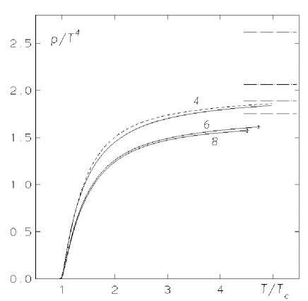
Figure 3: Rescaled pressure of SU(3) lattice gauge theory, from Boyd:1996bx , where $T_{c}$ is the transition temperature, and $N_{\tau}=4,6,8$.

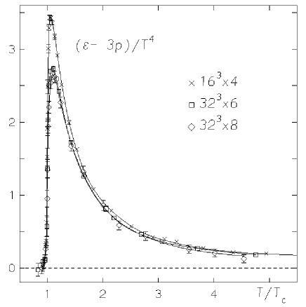
Figure 4: Rescaled anomaly of SU(3) lattice gauge theory, from Boyd:1996bx

II.7 Other approaches

Pisarski Pisarski:2006hz has observed from lattice data Boyd:1996bx that $(e-3p)/T^{4}\times T^{2}$ is approximately constant in a broad range above $T_{c}$. From this and physical reasoning he obtained the formula

$$p_{\rm pure\;glue}(T)\approx f_{\rm pert}(T^{4}-T_{c}^{2}T^{2}).$$ (17)

It is notable that no $T^{3}$ correction is apparent.

An active area of research is the AdS/CFT duality Maldacena:1997re and AdS/QCD duality Aharony:1999ti , including in particular duality at finite temperature (for a pedagogical introduction see Peeters:2007ab ). In this connection it is interesting to note that a formula similar to Pisarski’s has recently been obtained from this duality and the (truncated) entropy density of the horizon of a deformed Euclidean $\text{AdS}_{5}$ black hole, Andreev:2007zv .

II.8 Comparison of Results

Knowing that perturbation theory is limited to some fixed order in $g$, we can still estimate how good the possible perturbative description actually is. Ways to judge this are to check whether contributions from higher orders are small compared to those from lower orders or to compare perturbative expressions to results of lattice calculations.

Unfortunately, both methods suggest that the convergence is extremely poor for temperatures of the order of several $T_{c}$, where $T_{c}$ is the transition temperature, and to obtain good convergence one has to look at least at the electroweak scale, Zhai:1995ac ; Kajantie:2002wa . A plot of the results of optimized perturbation theory are given in fig. 5.

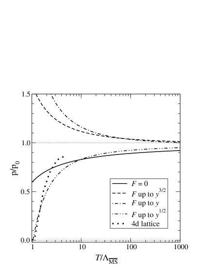
Figure 5: The convergence of an (optimized) perturbation series for “long-distance contribution” to the pressure, from Kajantie:2000iz . The order of the expansion is characterized by the dimensionless parameter $y\sim\frac{g^{2}T^{2}}{g_{3}^{4}}$, where $g_{3}^{2}$ denotes the gauge coupling in the effective three-dimensional theory. The perturbative contribution $F$ to the free energy contains a factor $\left(\frac{g_{3}^{2}}{T}\right)^{3}$, inclusion of lower powers of $y$ corresponds to higher orders in perturbation theory.

It has been conjectured, Laine:2003ay , that the results of order $g^{6}$ are not significantly changed by higher orders (since one can hope to have obtained at order $g^{6}$ the main contribution from each scale; perhaps also due to the fact that originally large terms of higher orders cancel against each other). To the knowledge of the authors, however, there is no strong evidence to support this conjecture.

From the existing data one cannot even exclude the unsettling possibiliy that for “physical” temperatures the perturbation series already begins to diverge at some order $n\leq 6$. This would mean that contributions from higher orders are of comparable magnitude to those of low order and no systematic cancellations occur. If this were indeed the case, we could not expect to have any reliable perturbative description for temperatures which are accessible in current experiments.

One should mention that there is an additional ambiguity in the perturbative results. All terms beyond the Stefan-Boltzmann contribution contain some power of the running coupling $g$. Thus, for all practical calculations there is some dependence on the scale $\mu$, at which $g(\mu)$ is evaluated. Traditionally, one chooses $\mu(T)=2\pi T$ in the high-temperature regime, but there are alternative approaches, for example application of the principle of minimal sensitivity, Stevenson:1981vj ; Blaizot:2003iq ; Inui:2005gu . We will discuss this question in more detail in section III.3.

III The Semiperturbative Approach

III.1 Equation of State from a Local Action

An alternative approach that combines nonperturbative elements with perturbative expansions has been developed in Zwanziger:2006sc ; Zwanziger:2007zz ; Zwanziger:2006wz , which we now briefly describe.

The basic physical idea is that the infrared divergences of finite-temperature perturbation theory do not arise when the domain of functional integration is cut-off at the Gribov horizon. The cut-off will be done in Coulomb gauge which is well adapted to finite-temperature calculations. Indeed both the gauge condition, $\partial_{i}A_{i}({\bf x},t)=0$, and the cut-off at the Gribov horizon are applied to 3-dimensional configurations on each time slice $t$, and are entirely independent of the temporal extent of the lattice $0\leq t\leq\beta$, where $\beta=1/kT$.

The functional cut-off at the Gribov horizon is effected at first by adding a non-local term $S_{NL}(A)$ to the action Zwanziger:1989mf ; Zwanziger:1993 . The non-local term then gets replaced by a local, renormalizable term $S_{L}$ in the action by means of an integration over a multiplet of auxiliary fermi and bose ghost pairs ,

$$\exp[-S_{NL}(A)]=\int\mathrm{d}\varphi\mathrm{d}\bar{\varphi}\mathrm{d}\omega\mathrm{d}\bar{\omega}\ \exp[-S_{L}(\varphi,\bar{\varphi},\omega,\bar{\omega})].$$ (18)

The BRST symmetry is explicitly broken by this term, an effect which, alternatively, may be interpreted as spontaneous BRST breaking Maggiore:1993wq . Although the breaking of BRST invariance precludes the definition of observables as elements of the cohomology of the BRST-operator, the eqivalence to the canonical formulation has been established Zwanziger:2006sc , thereby ensuring the physical foundation of the approach, including unitarity. Here the physicality of the Coulomb gauge plays an essential role.

The new term in the action depends on a mass parameter $m$ which appears in the Lagrangian density

$${\cal L}_{m} = -{m^{4}\over 2Ng^{2}}(D-1)(N^{2}-1)$$

$$+{m^{2}\over(2N)^{1/2}g}\ [\ D_{i}(\varphi-\bar{\varphi})_{i}+g(D_{i}c\times\bar{\omega}_{i})\ ]^{aa}.$$

The adjoint part of the Bose ghost $(\varphi-\bar{\varphi})_{i}$ mixes with the gauge field $A_{i}$ through the term $D_{i}(\varphi-\bar{\varphi})_{i}=(\partial_{i}+gA_{i}\times)(\varphi-\bar{\varphi})_{i}$. At tree level one obtains a gluon propagator,

$$D={1\over k_{0}^{2}+E^{2}(\boldsymbol{k})},$$ (20)

that satisfies the Gribov dispersion relation

$$E(\boldsymbol{k})=\sqrt{\boldsymbol{k}^{2}+\frac{m^{4}}{\boldsymbol{k}^{2}}}.$$ (21)

The functional cut-off at the Gribov horizon imposes the condition that the free energy $W$ or quantum effective action $\Gamma$ be stationary with respect to $m$,

$${\partial W\over\partial m}=-{\partial\Gamma\over\partial m}=0.$$ (22)

This “horizon condition” has the form of a non-perturbative gap equation that determines the Gribov mass $m=m(T,\Lambda_{QCD})$, and thereby provides a new vacuum, around which a perturbative expansion is again possible.

The most powerful non-perturbative methods available are called for to solve this system. However in the present work we shall modestly investigate a semi-perturbative method Zwanziger:2006sc , in which one calculates all quantities perturbatively in $g$, including $\Gamma$, taking $m$ to be a quantity of order $g^{0}$, and then one substitutes for $m$ the non-perturbative solution to the gap equation (22). We shall find that this method can be a good approximation only at extremely high energies. Nevertheless as a matter of principle, it is a significant success that for thermodynamic observables this procedure gives finite results precisely at the order, $g^{6}$ at which ordinary perturbation theory diverges.

III.2 The Gap Equation

In lowest non-trivial order in the semi-perturbative method Zwanziger:2006sc , the gap equation (22) reads after separation in an $m^{*}$-dependent and a $T$-dependent part

$$f\left(m^{*}\right) =y(T)$$ (23)

$$f\left(m^{*}\right) :=\frac{1}{2}\ln\frac{1}{m^{*}}+\int_{0}^{\infty}\frac{\mathrm{d}x}{u(x)}\,\frac{1}{\mathrm{e}^{m^{*}u(x)}-1}$$ (24)

$$y(T) :=\frac{3\pi^{2}}{N\,g^{2}(\mu)}-\frac{1}{4}\,\ln\frac{\mathrm{e}\mu^{2}(T)}{2\,T^{2}}\,.$$ (25)

where $m^{*}\equiv m_{r}=m/T$ is the rescaled Gribov mass and

$$u(x)\equiv\sqrt{x^{2}+\frac{1}{x^{2}}}\,$$ (26)

is the reduced dispersion relation. An important source of ambiguity, shared with other (semi)perturbative approaches, is the choice of the temperature-dependent scale $\mu(T)$ at which the coupling $g$ is evaluated.

III.3 Choice of the Renormalization Scale

We consider the coupling $g^{2}(\mu)$ at some renormalization scale $\mu(T)$. For a certain temperature $T$, the optimal renormalization scale should be chosen equal to the scale that governs the behaviour of the system. For field theory at high temperatures, this scale is expected to be equal to the lowest Matsubara frequency, i.e. $2\pi T$; for small $T$ it should be constant.

Since we are considering a confining theory with a mass gap, for low temperatures the optimal renormalization scale is not expected to go to to zero. For a system at very low (even zero) temperature, the most characteristic scale is not the very small average kinetic energy, but instead the mass of the lightest physical object, which is some bound state (a hadron in full QCD, a glueball in pure gauge theory). Actually, as long as we are in the confining region (i.e. below $T=T_{\mathrm{c}}$), the mass of bound states will always be “more important” than the thermal energy.

These restrictions, together with some conditions of “naturalness”, can be summarized by demanding that the renormalization scale $\mu(T)$ should fulfill:

$$\begin{array}[]{clcl}\text{(I)}&\mu(T)\approx\mu_{0}=\text{const}&&\text{for}\;T\ll T_{\mathrm{c}},\\[3.0pt] \text{(II)}&\mu(T)\approx 2\pi T&&\text{for}\;T\gg T_{\mathrm{c}},\\[3.0pt] \text{(III)}&\text{continuous},&&\\[3.0pt] \text{(IV)}&\text{monotonically rising}&&\text{for all}\;T,\\[3.0pt] \text{(V)}&\text{convex}&&\text{for all}\;T\end{array}$$

Conditions (I) and (II) might be replaced or supplemented by the asymptotic conditions

$$\begin{array}[]{cl}\text{(I')}&\displaystyle\lim_{T\to 0}(\mu(T)-\mu_{0})=0\,,\qquad\lim_{T\to 0}\frac{\mu(T)-\mu_{0}}{T}=0\,,\\[9.0pt] \text{(II')}&\displaystyle\lim_{T\to\infty}T^{n}\left(\mu(T)-2\pi T\right)=0\quad\text{for all}\;n\in\mathbb{N}_{0}\end{array}$$ (27)

Due to the phase transition at $T=T_{\mathrm{c}}\approx\Lambda_{\mathrm{QCD}}$, a simple choice is

$$\mu(T)=\begin{cases}\mu_{0,\mathrm{l}}(T):=2\pi\Lambda_{\overline{MS}}&\mathrm{for}\;T<\Lambda_{\overline{MS}}\\ \mu_{0,\mathrm{h}}(T):=2\pi T&\mathrm{for}\;T\geq\Lambda_{\overline{MS}}\,.\end{cases}$$ (28)

This choice is supported by the fact that $2\pi\Lambda_{\overline{MS}}$ is in the order of magnitude of glueball masses. Another reasonable choice is

$$\mu(T)=2\pi T+2\pi\,\Lambda_{\overline{MS}}\,\mathrm{e}^{-T/\Lambda_{\overline{MS}}}\,.$$ (29)

This form, however, is less favorable for numerical reasons, thus we have exclusively used (28) in the numerical studies performed in section III.4. Both forms are plotted in fig. 6.

Figure 6: The choices (28) and (29) for the renormalization scale $\mu(T)$, displayed together with the asymptotics $\mu_{0,\mathrm{l}}=2\pi\Lambda_{\mathrm{QCD}}$, $\mu_{0,\mathrm{h}}=2\pi T$. In addition we show $\frac{\mu(T)}{T}$ and $\mu^{\prime}=\frac{\mathrm{d}\mu}{\mathrm{d}T}$.

Another ansatz, used especially in functional calculations, Maas:2005hs , is a ’t Hooft-like scaling

$$g^{2}(\mu(T))\,T=\text{const}\,,$$ (30)

which, at one-loop level, corresponds to an exponential growth $\mu(T)=\mu_{0}\,\mathrm{e}^{\alpha T}$ with some positive constant $\alpha$. This choice provides a smooth infinite-temperature limit, but does not respect condition (II), and has not been used in the current article.

III.4 Calculational Methods

The gap equation (23) is an implicit equation for $m^{*}(T)$, which, in constrast to “genuine” integral equations, can be solved independently for each temperature $T$. Our results have been obtained in Mathematica by combining a numerical equation solver with adaptive Gauß-Legendre integration.

The derivatives necessary to obtain anomaly and bulk viscosity (see equations (45) and (50)) can be done either numerically or analytically. The second way unfortunately involves additional integrals, which can again only be evaluated numerically. (See appendix A for details.)

While both methods are potentially susceptible to numerical problems, they are of very different nature. Actually, the results of both methods agree remarkably well, inspiring confidence in the stability of the result.

All calculations directly involving $T$ have been performed on logarithmic temperature scale. This allows direct implementation of logarithmic derivatives, reduces numerical errors as compared to calculations on a linear scale and enables one to reach significantly higher temperatures.

For all quantities under consideration, we could obtain asymptotic expressions by expansion in the coupling $g^{2}$. In general, we use, Laine:2005ai ,

$$\frac{1}{g^{2}(\mu)} \overset{2\text{-loop}}{=}2b_{0}\,\ln\frac{\mu}{\Lambda_{\overline{\text{MS}}}}+\frac{b_{0}}{b_{1}}\,\ln\left(2\,\ln\frac{\mu}{\Lambda_{\overline{\text{MS}}}}\right)\,,$$ (31)

$$\mu\,\frac{\mathrm{d}g^{2}}{\mathrm{d}\mu} =\beta(g^{2})\overset{2\text{-loop}}{=}\frac{\beta_{0}}{(4\pi)^{2}}\,g^{4}(\mu)+\frac{\beta_{1}}{(4\pi)^{4}}\,g^{6}(\mu)$$ (32)

with the coefficients

$$\beta_{0} \equiv-2\,(4\pi)^{2}\,b_{0}=\frac{-22\,C_{A}+8T_{f}}{N}$$

$$\overset{\mbox{\footnotesize pure SU(3)}}{=}\;-22\,,$$ (33)

$$\beta_{1} \equiv-2\,(4\pi)^{4}\,b_{1}=\frac{-68C_{A}^{2}+40C_{A}T_{f}+24C_{f}T_{f}}{N}$$

$$\overset{\mbox{\footnotesize pure SU(3)}}{=}\;-204$$ (34)

and the group-theoretical factors $C_{A}=N$ and $C_{F}=N^{2}-1$. $T_{f}$ is equal to half the number of quark flavors and thus vanishes in pure gauge. While the results in subsection III.5 are given for the one-loop form (easily obtained by setting $\beta_{1}=b_{1}=0$ in (31) and (32)), there are only minor changes when switching to the two-loop form.

III.5 Results

We now summarize the results obtained by numerically solving the gap equation and the corresponding asymptotic expressions.

III.5.1 Gribov Mass

Solving the gap equation yields the Gribov mass $m(T)$. An expansion gives to leading order in $g^{2}$

$$m^{*}(T)\sim{N\over 2^{3/2}\ 3\ \pi}\ g^{2}(\mu)\,.$$ (35)

The numerical result and this asymptotic form are displayed in fig. 7. The agreement is excellent down to the phase transition (below which the formalism is probably not applicable anyhow), thus higher-order corrections to the Gribov mass are small.

(a)
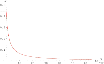
(b)

Figure 7: The rescaled Gribov mass $m^{*}=\frac{m}{T}$: (a) solid – numerical solution, dotted – asymptotic expression from (35); (b) relative deviation $\Delta m^{*}_{\mathrm{rel}}=(m^{*}_{\mathrm{num}}-m^{*}_{\mathrm{asy}})/m^{*}_{\mathrm{asy}}$

III.5.2 Free Energy and Pressure

For the pressure $p$ and the free energy $w$ we obtain

$$\frac{p}{T^{4}}\equiv\frac{w}{T^{3}} =(N^{2}-1)\,\left[\frac{3}{2N}\,\frac{{m^{*}}^{4}}{g^{2}(\mu)}+\frac{1}{3\pi^{2}T^{4}}\,K(m)\right]\,,$$ (36)

$$K(m) :=\int_{0}^{\infty}\frac{\mathrm{d}k}{E(k)}\,\frac{k^{4}-m^{4}}{\mathrm{e}^{\beta E(k)}-1}\,,$$ (37)

with $k=\left|\boldsymbol{k}\right|$. An expansion for $K(m)$ is not completely straightforward due to a nonanalyticity in $m^{4}$, but, as shown in Zwanziger:2006sc , it can be performed and yields the asymptotic expression

$$w\sim(N^{2}-1){\pi^{2}\over 45}\ \left(1-{5\over 18}\left({Ng^{2}\over 4\pi^{2}}\right)^{3}\right)\ T^{3}\,.$$ (38)

The full solution and the asymptotic form are given in fig. 8, where we have subtracted the Stefan-Boltzmann part, denoted by $w_{\text{SB}}$. In contrast to the case of $m$, higher-order corrections are obviously not small for $w$ since agreement between the full (numerical) and the asymptotic result is not good below $T\approx 10^{6}\,\Lambda_{\bar{MS}}$.

(a)
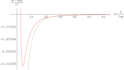
(b)

Figure 8: The rescaled reduced free energy $w_{r}-w_{\text{r,SB}}$: (a) solid – numerical solution, dotted – asymptotic expression from (38); (b) relative deviation $\Delta w_{\mathrm{r,rel}}=(w_{\mathrm{r,num}}-w_{\mathrm{r,asy}})/(w_{\mathrm{r,asy}}-w_{\text{r,SB}})$

It is instructive to see that $K(m)$ can also be evaluated by using an intermediate cutoff. While more cumbersome, this method allows us to identify contributions from different scales and thus gives some idea how to relate this result to the one obtained by effective theory approaches (see section II.4).

To do this, we introduce a cutoff $\Lambda$ with $m\ll\Lambda\ll T$, which separates contributions from the scale $m\sim g^{2}T$ and from the scale $2\pi T$. Doing so, we obtain

$$K(m)=\underbrace{\int_{0}^{\Lambda}\frac{\mathrm{d}k}{E(k)}\,\frac{k^{4}-m^{4}}{\mathrm{e}^{\beta E(k)}-1}}_{K_{1}}+\underbrace{\int_{\Lambda}^{\infty}\frac{\mathrm{d}k}{E(k)}\,\frac{k^{4}-m^{4}}{\mathrm{e}^{\beta E(k)}-1}}_{K_{2}},$$ (39)

where

$$K_{1} =m^{4}\int_{0}^{\Lambda/m}\mathrm{d}x\,\frac{x^{4}-1}{u(x)\,(\mathrm{e}^{\beta mu(x)}-1)}$$

$$\approx m^{3}T\int_{0}^{\Lambda/m}\mathrm{d}x\,\frac{x^{4}-1}{u^{2}(x)}=m^{3}T\int_{0}^{\Lambda/m}\mathrm{d}x\,x^{2}\frac{x^{4}-1}{x^{4}+1}$$

$$=m^{3}T\left\{\int_{0}^{\Lambda/m}\mathrm{d}x\,x^{2}-2\int_{0}^{\Lambda/m}\frac{x^{2}}{x^{4}+1}\,\mathrm{d}x\right\}\,.$$ (40)

The first integral is trivial; for the second we can replace the upper limit $\Lambda/m$ by $\infty$ and apply residue calculus to obtain

$$K_{1}=\frac{T}{3}\,\Lambda^{3}-\frac{\pi}{\sqrt{2}}\,m^{3}\,T\,.$$ (41)

For $K_{2}$ we obtain

$$K_{2} \approx\int_{\Lambda}^{\infty}\frac{\mathrm{d}k}{k}\,\frac{k^{4}}{\mathrm{e}^{\beta k}-1}=T^{4}\int_{\Lambda/T}^{\infty}\mathrm{d}y\,\frac{y^{3}}{\mathrm{e}^{y}-1}$$

$$=T^{4}\left\{\int_{0}^{\infty}\mathrm{d}y\,\frac{y^{3}}{\mathrm{e}^{y}-1}-\int_{0}^{\Lambda/T}\mathrm{d}y\,\frac{y^{3}}{\mathrm{e}^{y}-1}\right\}\,.$$ (42)

The first integral is the well-known Planck integral. In the second one we can again expand the exponential, since $y\leq\frac{\Lambda}{T}\ll 1$, and obtain

$$K_{2}\approx T^{4}\,\left\{\frac{\pi^{4}}{15}-\int_{0}^{\Lambda/T}\mathrm{d}y\,y^{2}\right\}=T^{4}\,\frac{\pi^{4}}{15}-\frac{T}{3}\,\Lambda^{3}\,.$$ (43)

This gives

$$K=K_{1}+K_{2}=T^{4}\,\frac{\pi^{4}}{15}-\frac{\pi}{\sqrt{2}}\,m^{3}\,T\,.$$ (44)

The cutoff-dependent parts in $K_{1}$ and $K_{2}$ precisely cancel, leaving a clear separation of the Stefan-Boltzmann contribution from $k\sim T$ and the contribution from the scale $k\sim m\sim g^{2}T$.

III.5.3 Energy and Anomaly

From the free energy or the pressure, we can calculate the rescaled anomaly via

$$A_{\mathrm{r}}=\frac{e-3p}{T^{4}}=T\,\frac{\mathrm{d}}{\mathrm{d}T}\frac{p}{T^{4}}=\frac{\mathrm{d}}{\mathrm{d}(\ln\frac{T}{\Lambda})}\frac{p}{T^{4}}\,,$$ (45)

(with some arbitrary scale $\Lambda$) since from (1), we have

$$T\,\frac{\mathrm{d}}{\mathrm{d}T}\frac{p}{T^{4}} \equiv T\,\frac{\mathrm{d}}{\mathrm{d}T}\frac{w}{T^{3}}=\frac{\frac{\partial w}{\partial T}}{T^{2}}-3\,\frac{w}{T^{3}}$$

$$=\frac{T^{2}\frac{\partial w}{\partial T}-3wT}{T^{4}}=\frac{e-3p}{T^{4}}\,.$$ (46)

It is also obvious that the energy can be directly obtained from the anomaly by using the relation $e=3p+A$. Thus we do not show separate graphs for $e$. From (45) it is also clear that all deviations from the Stefan-Boltzmann pressure $p_{\text{r,SB}}=\frac{\pi^{4}}{15}$ are encoded in the anomaly, since integration gives

$$p_{\text{r}}(T)=p_{\text{r,SB}}-\int_{T}^{\infty}\frac{A_{\text{r}}(T^{\prime})}{T^{\prime}}\,\mathrm{d}T^{\prime}\,.$$ (47)

From (38), (45), and (32) we obtain

$$A_{\mathrm{r}}\sim-(N^{2}-1)\frac{N^{3}}{3456\,\pi^{4}}\,g^{4}(\mu)\beta(g^{2})\frac{T}{\mu}\,\frac{\mathrm{d}\mu}{\mathrm{d}T}\,.$$ (48)

for the asymptotic expansion. The numerical result and the asymptotic form are shown in fig. 9. Again higher-order corrections are large except for extremely high temperatures.

(a)
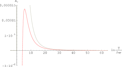
(b)

Figure 9: The rescaled anomaly $A_{r}$: (a) solid – numerical solution, dotted – asymptotic expression from (48); (b) relative deviation $\Delta A_{\mathrm{r,rel}}=(A_{\mathrm{r,num}}-A_{\mathrm{r,asy}})/A_{\mathrm{r,asy}}$

III.5.4 Bulk Viscosity

In formula (4) there is one ambiguity, the choice of the scale $\omega_{0}$. According to Karsch:2007jc a reasonable range of values is $\omega_{0}=(0.5\div 1.5)$ GeV. Neglecting the perturbative contribution from $\varepsilon_{V}$, we obtain

$$\zeta=\frac{1}{9\,\omega_{0}}\,T^{5}\,\frac{\mathrm{d}}{\mathrm{d}T}\frac{e-3p}{T^{4}}\,.$$ (49)

The rescaled bulk viscosity is given by

$$\zeta_{\text{r}}=\frac{1}{9\,\omega_{0}}\,T\,\frac{\mathrm{d}}{\mathrm{d}T}A_{\text{r}}\,.$$ (50)

In the asymptotic expression, correction terms originating from $\frac{T}{\mu}\,\frac{\mathrm{d}\mu}{\mathrm{d}T}$ become quite complicated. Since they are relatively unimportant for reasonable choice of $\mu(T)$ (and even vanish identically for the simple form (28)) we only give the simplified expression, where we have set $\frac{T}{\mu}\,\frac{\mathrm{d}\mu}{\mathrm{d}T}=1$,

$$\zeta_{\text{r}} \sim-\frac{1}{9\,\omega_{0}}\,\frac{N^{3}\,(N^{2}-1)}{3456\,\pi^{4}}$$

$$\qquad\left\{2\,g^{2}(\mu)\,\,\beta(g^{2})+g^{4}(\mu)\,\frac{\mathrm{d}\beta(g^{2})}{\mathrm{d}g^{2}}\right\}\,\beta(g^{2}).$$ (51)

The full expression is derived in appendix B. Graphs for the numerical solution and the asymptotic expression are shown in fig. 10 for the choice $\omega_{0}=5\Lambda_{\overline{\text{MS}}}$.

(a)
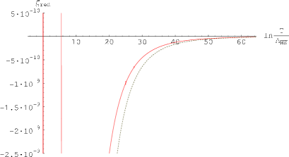
(b)

Figure 10: The rescaled bulk viscosity: (a) solid – numerical solution $\zeta_{\mathrm{r,num}}$, dotted – asymptotic expression $\zeta_{\mathrm{r,asy}}$ from (48); (b) relative deviation $\Delta\zeta_{\mathrm{r,rel}}=(\zeta_{\mathrm{r,num}}-\zeta_{\mathrm{r,asy}})/\zeta_{\mathrm{r,asy}}$

The behaviour close to $T=\Lambda_{\bar{MS}}$ is strongly influenced by the choice of $\mu(T)$. Apart from that however the viscosity $\zeta_{\text{r}}$ rises significantly when the temperature approaches the critical temperature from above, in agreement with Karsch:2007jc .

IV Discussion

IV.1 Access to the nonperturbative sector

Various results make clear that finite-temperature QCD contains in principle a perturbatively accessible sector, which, starting at order $(g^{2}T)^{3}$, interacts with a genuine nonperturbative sector. At least formally an expansion in powers of the coupling $g$ is possible also for non-perturbative contributions.

According to Gribov’s confinement scenario, Gribov:1977wm ; Zwanziger:1991gz ; Zwanziger:1992 , the vicinity of the Gribov horizon dominates the nonperturbative aspects of the theory. So correctly taking into account this region should give access to the nonperturbative sector of the theory at high temperatures also. Indeed, the cutoff at the Gribov horizon employed in this article gives a finite nonperturbative contribution to the free energy at order $g^{6}$, where the nonperturbative sector of the theory begins to spoil direct perturbative approaches.

The nonperturbative sector (described by MQCD in the picture of section II.4) is also accessible to lattice calculations. Comparison of our analytic result (38) with the lattice expressions (15) and (16) gives

$$w_{\text{np, analyt}}^{(6)} =-\frac{(N^{2}\!-\!1)\,N^{3}}{10\,368\,\pi^{4}}g^{6}T^{3}\,,$$ (52)

$$w_{\text{np, lattice}}^{(6)} =-\frac{(N^{2}\!-\!1)\,N^{3}}{1\,280\,\pi^{4}}(1\pm 4)g^{6}T^{3}\,.$$ (53)

These results are compatible, though the errors of the lattice calculations are too large at the moment to allow a definite statement about the quality of agreement.

IV.2 Convergence of the series?

As already mentioned in section II.8, the convergence of perturbation series is extremely poor for temperatures $\mathcal{O}(\text{GeV})$ or below. As discussed in Blaizot:2003iq , this can be traced back to the poor convergence of contributions from the EQCD sector, which begin to contribute at order $g^{3}$.

A similar behaviour seems to be true for the contribution from MQCD. While a formal expansion in $g$ is possible (and for very high temperatures $T\geq 10^{10}\text{GeV}$ the agreement is reasonably good), the expansion has little to do with the full result for low temperatures. From the low-temperature graphs displayed in figs. 11 to 13 it is likely that higher-order corrections cannot be small compared to the leading term.

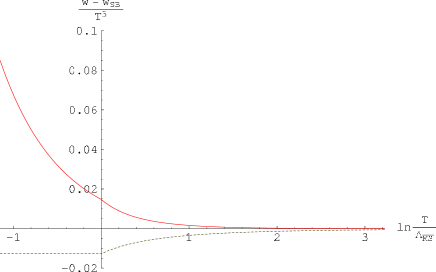
Figure 11: The rescaled free energy in the low-temperature region (solid – numerical solution, dotted – asymptotic expression from (48))

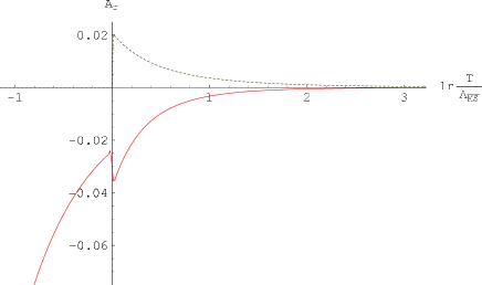
Figure 12: The rescaled anomly $\frac{e-3p}{T^{4}}$ in the low-temperature region (solid – numerical solution, dotted – asymptotic expression from (48))

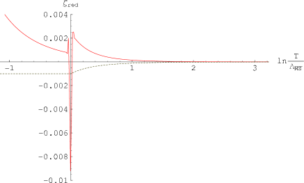
Figure 13: The rescaled bulk viscosity in the low-temperature region (solid – numerical solution, dotted – asymptotic expression from (48))

This suggests that either the convergence is extremely poor or that there is even no convergence at all. The latter would not be completely unexpected. It is well known that in quantum field theory series obtained by expansion in the coupling are rarely convergent, but at best asymptotic (and usually even this cannot be proven).

Assuming that expansion in $g$ of the QCD free energy yields a divergent asymptotic series would give the following scenario: For each temperature $T$ one can expect that an “optimal order” $n$ exists beyond which the series leaves the “path of apparent convergence”. For low temperatures and thus large couplings this order may be so small that no partial sum of the perturbation series can serve as a satisfactory approximation.

IV.3 Further Steps

Our studies leave open several questions that are worth further investigation. While the analytic result (52) is compatible with the lattice result (53), a reduction of the errors of the latter would be highly desirable. (Unfortunately the errors would have to be reduced about one order of magnitude, a task which would require considerable computational resources.)

On the analytic side, higher-order calculations in the semi-perturbative formalism could help to further clearify the connection of our approach to the sequence of theories discussed in subsection II.4. They could also help to reveal if (52) is indeed the full contribution to order $g^{6}$ from the magnetostatic sector or if there are additional contributions from (formally) higher orders as well, which are not present in the lowest-order approximation to the gap equation (23).

Such calculations could also shed some more light on the question of (apparent) convergence, as just discussed in subsection IV.2. Of course also determination of the full $g^{6}$ contribution to the free energy (conceptually possible in the framework of effective theories) would be very helpful for further statements about convergence issues.

Our results indicate that the semi-perturbative method of calculation is reliable only at extremely high $T$. A more advanced approach to the nonperturbative sector could involve solving the Dyson-Schwinger equation for the system with local action and auxiliary fermi and bose ghost pairs Zwanziger:2006sc or, alternatively, studying bound-state equations for glueballs in MQCD. Those objects, which determine higher-order contributions from this sector are closely related (though not strictly identical) to chromomagnetic glueballs in the four-dimensional theory.

V Summary and Outlook

We first presented a short synopsis on current problems in thermal QCD, where we also reviewed several methods to approach them, including consecutive effective field theories, as proposed in Braaten:1995cm .

Then, using the local action proposed in Zwanziger:2006sc , we obtained nonperturbative contributions to several thermodynamic observables, including free energy, anomaly and bulk viscosity. Being directly related to other nonperturbative approaches (like magnetostatic QCD), this method provides a framework for purely analytical studies beyond the limits of thermal perturbation theory, without the necessity of lattice calculations (neither in the full nor in an effective theory.)

While for each quantity we were able to obtain the leading coefficient of the expansion in the coupling $g$, we also noticed that higher-order corrections have to be large in order to accomodate the numerical results. This is one more sign that, in thermal QCD, expansion in the coupling cannot be expected to give reliable approximations except for extremely high temperatures.

While results are promising, further investigations are necessary to clearify the limits of this method, illuminate further the relation to other approaches and perhaps extract general information about the quality of series expansions in thermal QCD.

Acknowledgements

K.L was supported by the Doktoratskolleg Hadronen im Vakuum, in Kernen und Sternen (FWF DK W1203-N08) and by the Graz Advanced School of Science (NAWI-GASS). He would like to express his thanks for the hospitality of New York University (NYU), where most of this work was done, and to Reinhard Alkofer for his support, in particular for making possible the stay at NYU.

The authors are especially grateful to Reinhard Alkofer for valuable comments and to Roman Scoccimarro for developing an early version of the numerical program used to solve the gap equation. They would like to thank Fritjof Karsch and Jürgen Engels for providing lattice data from Boyd:1996bx and Mikko Laine for making them aware of references Hietanen:2004ew ; Hietanen:2006rc ; DiRenzo:2006nh ; Schroder:2002re ; Schroder:2003uw .

Appendix A The Anomaly from an Analytic Derivative

We now show how the anomaly can be obtained without the necessity for numerical differentiation. In the following, we always understand $g^{2}=g^{2}(\mu)$ and $\mu=\mu(T)$.

One-loop expansion of the gap equation gives for the rescaled pressure

$$\frac{p}{T^{4}}\equiv\frac{w}{T^{3}}=(N^{2}-1)\,\left[\frac{3}{2N}\,\frac{{m^{*}}^{4}}{g^{2}(\mu)}+\frac{1}{3\pi^{2}}\,K(m^{*})\right]$$ (54)

with $K(m^{*})={m^{*}}^{4}\,I(m^{*})$ and

$$I(m^{*}):=\int_{0}^{\infty}\frac{\mathrm{d}x}{u(x)}\,\frac{x^{4}-1}{\mathrm{e}^{m^{*}u(x)}-1}\,,$$ (55)

using the reduced dispersion relation (26). From this, we obtain

$$A_{\mathrm{r}} =T\,\,\frac{\mathrm{d}}{\mathrm{d}T}\frac{p}{T^{4}}$$

$$=(N^{2}-1)\left[\frac{3}{2N}\,T\,\frac{\mathrm{d}}{\mathrm{d}T}\frac{{m^{*}}^{4}}{g^{2}}+\frac{1}{3\pi^{2}}\,T\,\frac{\partial K(m^{*})}{\partial T}\right]$$

$$=3\,\frac{N^{2}-1}{2N}\left[-\frac{{m^{*}}^{4}}{g^{4}}\,T\,\frac{\mathrm{d}g^{2}}{\mathrm{d}T}+\frac{4\,{m^{*}}^{3}}{g^{2}}\,T\,\frac{\mathrm{d}m^{*}}{\mathrm{d}T}\right]$$

$$\qquad+\frac{N^{2}-1}{3\pi^{2}}\,T\,\frac{\partial K(m^{*})}{\partial T}\,.$$ (56)

The derivative of $g^{2}$ with respect to $T$ be easily calculated using the $\beta$-function,

$$T\,\frac{\mathrm{d}(g^{2})}{\mathrm{d}\mu}=\frac{T}{\mu}\,\mu\,\frac{\mathrm{d}(g^{2})}{\mathrm{d}\mu}=\frac{T}{\mu}\,\beta(g^{2})\,.$$ (57)

From this, we obtain

$$T\,\frac{\mathrm{d}g^{2}(\mu)}{\mathrm{d}T} =\frac{T}{\mu}\,\mu\,\frac{\mathrm{d}g^{2}(\mu)}{\mathrm{d}\mu}\,\frac{\mathrm{d}\mu(T)}{\mathrm{d}T}=\beta(g^{2}(\mu))\,\frac{T}{\mu}\,\frac{\mathrm{d}\mu(T)}{\mathrm{d}T}\,.$$ (58)

For the last term in (56) we have

$$T\,\frac{\partial K(m^{*})}{\partial T} =T\,\frac{\partial m^{*}}{\partial T}\,\frac{\partial K(m^{*})}{\partial m^{*}}\,$$ (59)

$$\frac{\partial K(m^{*})}{\partial m^{*}} =4\,{m^{*}}^{3}\,I(m^{*})-{m^{*}}^{4}\,L(m^{*})\,$$ (60)

$$L(m^{*}) =\int_{0}^{\infty}\mathrm{d}x\,\frac{(x^{4}-1)\,\mathrm{e}^{m^{*}u(x)}}{(\mathrm{e}^{m^{*}u(x)}-1)^{2}}\,.$$ (61)

We obtain $T\,\frac{\partial m^{*}}{\partial T}$ by differentiating the gap equation $f\left(m^{*}\right)=y(T)$ with respect to $T$, where

$$f\left(m^{*}\right) =\frac{1}{2}\ln\frac{1}{m^{*}}+\int_{0}^{\infty}\frac{\mathrm{d}x}{u(x)}\,\frac{1}{\mathrm{e}^{m^{*}u(x)}-1}\,,$$ (62)

$$y(T) =\frac{3\pi^{2}}{N\,g^{2}(\mu)}-\frac{1}{4}\,\ln\frac{\mathrm{e}\mu^{2}(T)}{2\,T^{2}}\,.$$ (63)

Since the left-hand side depends on $T$ only implicitly via $m^{*}$, we have

$$\frac{\mathrm{d}}{\mathrm{d}T}f(m^{*}) =\frac{\mathrm{d}f}{\mathrm{d}m^{*}}\,\frac{\mathrm{d}m*}{\mathrm{d}T}=\left[-\frac{1}{2}\,\frac{1}{m^{*}}-J(m^{*})\right]\,\frac{\mathrm{d}m^{*}}{\mathrm{d}T}\,,$$ (64)

$$J(m^{*}) =\int_{0}^{\infty}\mathrm{d}x\,\frac{\mathrm{e}^{m^{*}u(x)}}{\left(\mathrm{e}^{m^{*}u(x)}-1\right)^{2}}\,.$$ (65)

Differention of the right-hand side yields

$$\frac{\mathrm{d}y(T)}{\mathrm{d}T} =\frac{\mathrm{d}}{\mathrm{d}T}\left[\frac{3\pi^{2}}{N\,g^{2}(\mu)}-\frac{1}{4}\,\ln\frac{\mathrm{e}\mu^{2}(T)}{2\,T^{2}}\right]$$

$$=-\frac{3\pi^{2}}{N\,g^{4}(\mu(T))}\,\frac{\mathrm{d}g^{2}(\mu)}{\mathrm{d}T}-\frac{\mathrm{d}}{\mathrm{d}T}\frac{1}{2}\,\ln\left(\sqrt{\frac{\mathrm{e}}{2}}\frac{\mu(T)}{T}\right)$$

$$=-\frac{3\pi^{2}}{N\,g^{4}(\mu(T))}\,\frac{1}{\mu(T)}\,\mu(T)\frac{\mathrm{d}g^{2}(\mu)}{\mathrm{d}T}$$

$$\quad-\frac{1}{2}\,\frac{T}{\mu(T)}\left(\frac{\frac{\mathrm{d}\mu}{\mathrm{d}T}}{T}-\frac{\mu}{T^{2}}\right)$$

$$=-\frac{1}{\mu(T)}\,\left\{\frac{3\pi^{2}}{N}\,\frac{\beta(g^{2})}{g^{4}(\mu)}\,\frac{\mathrm{d}\mu}{\mathrm{d}T}+\frac{1}{2}\left(\frac{\mathrm{d}\mu}{\mathrm{d}T}-\frac{\mu}{T}\right)\right\}\,.$$ (66)

The second term inside the curly brackets is a measure for the deviation from the asymptotic behaviour; in the asymptotic regime with $\mu(T)=2\pi T$, the above expression simplifies to

$$\left.\frac{\mathrm{d}y(T)}{\mathrm{d}T}\right|_{\mathrm{asympt}}=-\frac{3\pi^{2}}{N}\,\frac{1}{T}\,\frac{\beta(g^{2}(2\pi T))}{g^{4}(2\pi T)}\,.$$ (67)

Collecting our results, we obtain

$$T\,\frac{\mathrm{d}m^{*}}{\mathrm{d}T} =\frac{T\,\frac{\mathrm{d}y}{\mathrm{d}T}}{-\frac{1}{2m^{*}}-J(m^{*})}$$

$$=\frac{T}{\mu(T)}\,\frac{1}{\frac{1}{2m^{*}}+J(m^{*})}$$

$$\cdot\left\{\frac{3\pi^{2}}{N}\,\frac{\beta(g^{2})}{g^{4}}\,\frac{\mathrm{d}\mu}{\mathrm{d}T}+\frac{1}{2}\left(\frac{\partial\mu}{\partial T}-\frac{\mu}{T}\right)\right\}\,,$$ (68)

and the rescaled anomaly is given by

$$A_{\mathrm{r}} =3\,\frac{N^{2}-1}{2N}\left[-\frac{{m^{*}}^{4}}{g^{4}}\,\beta(g^{2})\,\frac{T}{\mu}\,\frac{\mathrm{d}\mu}{\mathrm{d}T}+\frac{4\,{m^{*}}^{3}}{g^{2}}\,T\,\frac{\mathrm{d}m^{*}}{\mathrm{d}T}\right]$$

$$\quad+\frac{N^{2}-1}{3\pi^{2}}\,\left(4\,{m^{*}}^{3}\,I(m^{*})-{m^{*}}^{4}\,L(m^{*})\right)\,T\,\frac{\mathrm{d}m^{*}}{\mathrm{d}T}\,.$$ (69)

Appendix B Asymptotic Bulk Viscosity

Keeping the full dependence on $\mu(T)$, we obtain for the bulk viscosity (49), again making use of (57),

$$\zeta =\frac{1}{9\,\omega_{0}}\,T^{5}\,\frac{\mathrm{d}}{\mathrm{d}T}\frac{e-3p}{T^{4}}$$

$$\sim-\frac{1}{9\,\omega_{0}}\,\frac{N^{3}\,(N^{2}-1)}{3456\,\pi^{4}}\,T^{5}\,\frac{\mathrm{d}}{\mathrm{d}T}g^{4}(\mu)\,\beta(g^{2})\frac{T}{\mu}\,\frac{\mathrm{d}\mu}{\mathrm{d}T}$$

$$\sim-\frac{1}{9\,\omega_{0}}\,\frac{N^{3}\,(N^{2}-1)}{3456\,\pi^{4}}\,T^{5}$$

$$\quad\Bigg{\{}\left[2\,g^{2}(\mu)\,\,\beta(g^{2})+g^{4}(\mu)\,\frac{\mathrm{d}\beta(g^{2})}{\mathrm{d}g^{2}}\right]\frac{\mathrm{d}(g^{2})}{\mathrm{d}\mu}\,\frac{\mathrm{d}\mu}{\mathrm{d}T}\,\frac{T}{\mu}\,\frac{\mathrm{d}\mu}{\mathrm{d}T}$$

$$\qquad+g^{4}(\mu)\,\beta(g^{2})\,\left[\frac{1}{\mu}\,\frac{\mathrm{d}\mu}{\mathrm{d}T}-\frac{T}{\mu^{2}}\,\left(\frac{\mathrm{d}\mu}{\mathrm{d}T}\right)^{2}+\frac{T}{\mu}\,\frac{d^{2}\mu}{\mathrm{d}T^{2}}\right]\Bigg{\}}$$

$$\sim-\frac{1}{9\,\omega_{0}}\,\frac{N^{3}\,(N^{2}-1)}{3456\,\pi^{4}}\,T^{4}\,g^{2}(\mu)\,\beta(g^{2})$$

$$\quad\Bigg{\{}\left[2\beta(g^{2})+g^{2}(\mu)\,\frac{\mathrm{d}\beta(g^{2})}{\mathrm{d}g^{2}}\right]\left(\frac{T}{\mu}\,\frac{\mathrm{d}\mu}{\mathrm{d}T}\right)^{2}$$

$$\qquad+g^{2}(\mu)\,\left[\frac{T}{\mu}\,\frac{\mathrm{d}\mu}{\mathrm{d}T}-\left(\frac{T}{\mu}\,\frac{\mathrm{d}\mu}{\mathrm{d}T}\right)^{2}+\frac{T}{\mu^{2}}\,\frac{d^{2}\mu}{\mathrm{d}T^{2}}\right]\Bigg{\}}\,.$$ (70)

References

- (1) E. V. Shuryak, Phys. Lett. B 78, 150 (1978) [Sov. J. Nucl. Phys. 28, 408.1978 YAFIA,28,796 (1978 YAFIA,28,796-808.1978)].
- (2) R. Hagedorn, Nuovo Cim. Suppl. 3, 147 (1965);
- (3) A. D. Linde, Phys. Lett. B 96, 289 (1980).
- (4) D. J. Gross, R. D. Pisarski and L. G. Yaffe, Rev. Mod. Phys. 53, 43 (1981).
- (5) E. V. Shuryak, Nucl. Phys. A 750, 64 (2005), arXiv:hep-ph/0405066
- (6) V. M. Bannur, Eur. Phys. J. C 11, 169 (1999) arXiv:hep-ph/9811397
- (7) E. Shuryak, J. Phys. Conf. Ser. 50, 62 (2006).
- (8) B. Müller and J. L. Nagle, Ann. Rev. Nucl. Part. Sci. 56, 93 (2006) arXiv:nucl-th/0602029
- (9) D. Zwanziger, Phys. Rev. D 76, 125014 (2007) arXiv:hep-ph/0610021
- (10) D. Zwanziger, Braz. J. Phys. 37, 127 (2007).
- (11) D. Zwanziger, AIP Conf. Proc. 892, 121 (2007) arXiv:hep-ph/0611150
- (12) V. N. Gribov, Nucl. Phys.B139, 1978.
- (13) I. Zahed and D. Zwanziger, Phys. Rev. D 61, 037501 (2000) [arXiv:hep:th/9905109].
- (14) D. Kharzeev and K. Tuchin, arXiv:0705.4280 [hep-ph].
- (15) S. G. Brown, Phys. Rev. 158, 5 (1967).
- (16) J. I. Kapusta and C. Gale, Cambridge Univ. Pr., Cambridge, (2006), p. 428.
- (17) E. V. Shuryak, Sov. Phys. JETP 47, 212 (1978) [Zh. Eksp. Teor. Fiz. 74, 408 (1978)].
- (18) S. A. Chin, Phys. Lett. B 78, 552 (1978).
- (19) J. I. Kapusta, Nucl. Phys. B 148, 461 (1979).
- (20) T. Toimela, Phys. Lett. B 124, 407 (1983).
- (21) P. Arnold and C. X. Zhai, Phys. Rev. D 50, 7603 (1994) arXiv:hep-ph/9408276
- (22) P. Arnold and C. x. Zhai, Phys. Rev. D 51, 1906 (1995) arXiv:hep-ph/9410360
- (23) C. x. Zhai and B. M. Kastening, Phys. Rev. D 52, 7232 (1995) arXiv:hep-ph/9507380
- (24) E. Braaten and A. Nieto, Phys. Rev. D 51, 6990 (1995) arXiv:hep-ph/9501375
- (25) T. Appelquist and R. D. Pisarski, Phys. Rev. D 23, 2305 (1981).
- (26) E. Braaten, Phys. Rev. Lett. 74, 2164 (1995) arXiv:hep-ph/9409434
- (27) K. Kajantie, M. Laine, K. Rummukainen and Y. Schroder, Phys. Rev. D 67, 105008 (2003) arXiv:hep-ph/0211321
- (28) Y. Schröder, Nucl. Phys. Proc. Suppl. 116, 402 (2003) arXiv:hep-ph/0211288
- (29) Y. Schröder, Nucl. Phys. Proc. Suppl. 129, 572 (2004) arXiv:hep-lat/0309112
- (30) M. Laine and Y. Schröder, JHEP 0503, 067 (2005) arXiv:hep-ph/0503061
- (31) Y. Schröder, arXiv:hep-ph/0410130
- (32) A. Hietanen, K. Kajantie, M. Laine, K. Rummukainen and Y. Schröder, JHEP 0501, 013 (2005) arXiv:hep-lat/0412008
- (33) A. Hietanen and A. Kurkela, JHEP 0611, 060 (2006), arXiv:hep-lat/0609015
- (34) F. Di Renzo, M. Laine, V. Miccio, Y. Schröder and C. Torrero, JHEP 0607, 026 (2006), arXiv:hep-ph/0605042
- (35) R. Alkofer and L. von Smekal, Phys. Rept. 353, 281 (2001) arXiv:hep-ph/0007355
- (36) A. Maas, J. Wambach, B. Gruter and R. Alkofer, Eur. Phys. J. C 37, 335 (2004) arXiv:hep-ph/0408074
- (37) A. Maas, J. Wambach and R. Alkofer, Eur. Phys. J. C 42, 93 (2005) arXiv:hep-ph/0504019
- (38) G. Boyd, J. Engels, F. Karsch, E. Laermann, C. Legeland, M. Lutgemeier and B. Petersson, Nucl. Phys. B 469, 419 (1996) arXiv:hep-lat/9602007
- (39) M. Okamoto et al. [CP-PACS Collaboration], Phys. Rev. D 60, 094510 (1999) arXiv:hep-lat/9905005
- (40) F. Gliozzi, J. Phys. A 40, F375 (2007) arXiv:hep-lat/0701020.
- (41) R. D. Pisarski, Phys. Rev. D 74, 121703 (2006) arXiv:hep-ph/0608242
- (42) J. M. Maldacena, Adv. Theor. Math. Phys. 2, 231 (1998) [Int. J. Theor. Phys. 38, 1113 (1999)] arXiv:hep-th/9711200
- (43) O. Aharony, S. S. Gubser, J. M. Maldacena, H. Ooguri and Y. Oz, Phys. Rept. 323, 183 (2000) arXiv:hep-th/9905111
- (44) K. Peeters and M. Zamaklar, Eur. Phys. J. ST 152, 113 (2007) arXiv:0708.1502[hep-ph]
- (45) O. Andreev, Phys. Rev. D 76, 087702 (2007) arXiv:0706.3120[hep-ph]
- (46) K. Kajantie, M. Laine, K. Rummukainen and Y. Schröder, Phys. Rev. Lett. 86, 10 (2001) arXiv:hep-ph/0007109
- (47) M. Laine, arXiv:hep-ph/0301011
- (48) P. M. Stevenson, Phys. Rev. D 23, 2916 (1981).
- (49) J. P. Blaizot, E. Iancu and A. Rebhan, Phys. Rev. D 68, 025011 (2003) arXiv:hep-ph/0303045
- (50) M. Inui, A. Niegawa and H. Ozaki, Prog. Theor. Phys. 115, 411 (2006) arXiv:hep-ph/0501277.
- (51) D. Zwanziger, Nucl. Phys. B 323, 513 (1989).
- (52) D. Zwanziger, Nucl. Phys. B 399, 477 (1993).
- (53) N. Maggiore and M. Schaden, Phys. Rev. D 50, 6616 (1994) arXiv:hep-th/9310111.
- (54) F. Karsch, D. Kharzeev and K. Tuchin, arXiv:0711.0914 [hep-ph].
- (55) D. Zwanziger, Nucl. Phys. B 364, 127 (1991).
- (56) D. Zwanziger, Nucl. Phys. B 378, 525 (1992).