Superdiffusion in a class of networks with marginal long-range connections

Abstract

A class of cubic networks composed of a regular one-dimensional lattice and a set of long-range links is introduced. Networks parametrized by a positive integer $k$ are constructed by starting from a one-dimensional lattice and iteratively connecting each site of degree $2$ with a $k$th neighboring site of degree $2$. Specifying the way pairs of sites to be connected are selected, various random and regular networks are defined, all of which have a power-law edge-length distribution of the form $P_{>}(l)\sim l^{-s}$ with the marginal exponent $s=1$. In all these networks, lengths of shortest paths grow as a power of the distance and random walk is super-diffusive. Applying a renormalization group method, the corresponding shortest-path dimensions and random-walk dimensions are calculated exactly for $k=1$ networks and for $k=2$ regular networks; in other cases, they are estimated by numerical methods. Although, $s=1$ holds for all representatives of this class, the above quantities are found to depend on the details of the structure of networks controlled by $k$ and other parameters.

I Introduction

Random walk in disordered environments is a much studied problem as it is a basic model in the theory of transport in heterogeneous media havlin ; bouchaud and it has features much different from those characteristic of homogeneous systems. In many cases, the diffusion law is altered in the way that the typical displacement of the random walker still grows as a power of time, i.e. $R(t)\sim t^{\nu}$, however, the diffusion exponent $\nu$ differs from the value $\nu=1/2$ characteristic of normal diffusion. In case of random walks with quenched random jump rates on regular lattices or random walks on fractal lattices (e.g. percolation clusters) the process is in general sub-diffusive, i.e. $\nu<1/2$ havlin ; bouchaud . The opposite case, $\nu>1/2$, where the particle is speeded up compared to normal diffusion, is much rarer. This phenomenon, called superdiffusion, arises e.g. in turbulent fluids swk , in chaotic transport in laminar fluid flows solomon or in systems of polymerlike breakable micelles oblu . In random walk models, superdiffusion can be induced by allowing long-range jumps: In the Lévy flight bouchaud , jumps of arbitrary length are executed with a probability that decays as a power of the length; in its “discretized” version, the Weierstrass walk, the possible jump lengths are integer powers of an integer $a>1$ weierstrass .

Another possibility for superdiffusion in case of random walks on a lattice is when long-range jumps occur only at certain sites of the lattice. In most cases, the underlying lattice is a union of a regular and a random graph, where the latter has arbitrarily long edges. Such graphs have been investigated in various aspects. As a variant of the small-world network model constructed by rewiring edges of a regular network ws , Newman and Watts have considered a one-dimensional lattice to which “shortcuts” between randomly chosen pairs of sites are added nw . In this model, shortest paths nw ; moukarzel , as well as spectral properties of the Laplacian monasson have been studied. Shortest paths or the diameter of d-dimensional lattices where long edges exist between pairs of sites with probabilities that decay algebraically with the distance have been studied by several authors for $d=1$ jespersen ; bb ; sc ; mam and for $d\geq 1$ coppersmith . Beside the above models, $n$-regular graphs of this type, where the degree of all nodes (i.e. the number of edges emanating from a node) is $n$, have been introduced, as well. The issue of decentralized algorithms for finding short paths has been considered by Kleinberg in a $d$-dimensional lattice where each site has a fixed number of directed edges to randomly chosen sites that are selected with power-law decaying probabilities kleinberg . Benjamini and Hoffman have studied minimal paths in $\omega$-periodic graphs, which are unions of periodic graphs over the integers bh . Recently, Boettcher et al. have introduced a hierarchical $3$-regular network consisting of a one-dimensional lattice and recursively constructed long-range links and calculated the random-walk dimension $d_{\rm rw}\equiv 1/\nu$ of this network boettcher .

In this paper, we shall consider networks composed of a one-dimensional lattice and an additional set of long links. Particularly, we focus on the intriguing situation when the tail of the distribution of edge-lengths is of the form $P_{>}(l)\sim\beta l^{-1}$. In this case, the diameter is conjectured to grow algebraically with the size of the network with a non-universal $\beta$-dependent exponent bb ; coppersmith . The aim of this work is to confirm this conjecture by explicit calculations and to probe whether the diffusion exponent in such networks displays a similar “marginal” behavior. For this purpose, we define a class of cubic (i.e. $3$-regular) networks with marginal edge-length distributions (i.e. $P_{>}(l)\sim l^{-1}$) and shall constructively demonstrate that the shortest-path dimension that characterizes the size-dependence of the diameter and the diffusion exponent are not exclusively determined by the power in the edge-length distribution but depend on the details of the structure of networks. The above two intrinsic properties of networks are calculated exactly in certain cases by means of a renormalization group method; in other cases, they are estimated by the numerical implementation of the renormalization procedure and by numerical simulation.

The rest of the paper is organized as follows. In Section II, a class of networks parametrized by a positive integer $k$ is defined and its general features are discussed. In Section III, networks with $k=1$ whereas in Section IV, networks with $k>2$ are investigated in detail. Results are discussed in Section V and a heuristic derivation of the relation to resistor networks is presented in the Appendix.

II General features

II.1 Construction of the networks

The networks to be studied in the subsequent sections have in common that they are all constructed in the following way. A one-dimensional open or periodic lattice with $N$ sites is given, where sites are numbered consecutively from $1$ to $N$. The degree of all sites is thus initially $2$ in the periodic lattice and all but site $1$ and $N$ in the open one. Sites of degree $2$ will be called in brief active sites. The links of this initial regular lattice will be termed short links in the followings in order to distinguish them from long links generated by the following procedure. Let us assume that $N$ is even and $k$ is a fixed positive integer. A pair of active sites is selected such that the number of active sites between them is $k-1$ and this pair is then connected by a (long) link. That means, for $k=1$, neighboring active sites are connected, for $k=2$ next-to-neighboring ones, etc. This step, which renders two active sites to sites of degree $3$, is then iterated until $2(k-1)$ active sites are left. These are then paired in an arbitrary way, which does not affect the exponents appearing in asymptotic relations in the limit $N\to\infty$. In the resulting network, all sites are of degree $3$ if the procedure starts from a periodic lattice whereas, in case of an open lattice, site $1$ and site $N$ remain of degree $1$. The networks generated in this way (or, more precisely, the ensembles of networks in case of random networks) are characterized by the number $k$ and by the way pairs are selected.

At some stage of the construction procedure, when the number of active sites is $N_{a}$, these sites are distributed homogeneously on a coarse-grained scale $\xi\gg 1/c$, where $c\equiv N_{a}/N$ is their number density. In other words, spacings between neighboring active sites have a rapidly decaying distribution with the expected value $1/c$. Thus, long links of length larger than $l$ are generated typically when $c$ is smaller than $1/l$ and we obtain for the distribution of lengths in an infinite network ($N\to\infty$): $P_{>}(l)\sim l^{-1}$. Disregarding regular networks (see Section III.2.1 and IV.2), where exclusively long links of length $l_{n}\sim\lambda^{n}$ ($\lambda>1$, $n=1,2,\dots$) form, the probability of a long link of length $l$ is thus inversely proportional to the square of the length: $p_{l}\sim l^{-2}$. Note, however, that not all edge lengths are realized in the construction procedure even for random networks. Namely, for $k=1$, only long links of odd length are produced.

II.2 Studied quantities

We are interested in two intrinsic properties of networks. Beside the distance $l$ measured on the underlying one-dimensional lattice, we also consider another metric: The chemical distance (or the length of the shortest path) $\ell$ between two sites is the minimum number of links that have to be traversed when going from one site to the other. We will see that, in the networks under study, the average length of shortest path between sites located in a distance $l$ grows algebraically with $l$ for large distances: $\overline{\ell(l)}\sim l^{d_{\rm min}}$, where the shortest-path dimension $d_{\rm min}<1$ is characteristic of the particular network. This dimension describes at the same time the finite-size scaling of the diameter $D(N)$ of a network, which is the maximum of chemical distances between any pairs of sites: $D(N)\sim N^{d_{\rm min}}$.

The other quantity of interest is the random-walk dimension of the network gaa ; havlin . We consider a continuous time random walk on (infinite) networks, where the walker can jump with unit rate to any of the sites connected with the site it resides. The random-walk dimension $d_{\rm rw}$ is defined through the relation $[\langle x^{2}(t)\rangle]_{\rm typ}\sim t^{2/d_{\rm rw}}$, where $x(t)$ denotes the displacement of the walker (measured on the underlying one-dimensional lattice) at time $t$ and $[\langle x^{2}(t)\rangle]_{\rm typ}\equiv\exp{\overline{\ln\langle x^{2}(t)\rangle}}$ is the “typical value” of $\langle x^{2}(t)\rangle$. Here, $\langle\cdot\rangle$ denotes the expected value for a fixed starting position in a fixed realization of the ensemble of networks, while the overbar stands for the average over starting positions and the ensemble of networks. Note that the expected value $\overline{\langle x^{2}(t)\rangle}$ does not exist if $t>0$ since the expected value of edge lengths is infinite (in infinite networks). This accounts for that the average of $\ln\langle x^{2}(t)\rangle$ is considered instead. The practical reason of the second averaging procedure is to eliminate random modulations which stem from the randomness of the structure of networks, whereas for regular networks, this averaging may be ignored.

II.3 Relation to resistor networks

The calculation of random-walk dimension is based on the well-known relation between the effective diffusion constant and the effective resistance of the equivalent resistor network bouchaud ; havlin . In the equivalent resistor network, each link has a (dimensionless) resistance $r_{i}$ related to the jump rate $w_{i}$ along that link via $r_{i}=1/w_{i}$. Considering networks built on an open lattice, the time $t$ needed for the walker to get from one end of the network (site $1$) to the other one (site $N$) is

$$t\sim N\tilde{r}$$ (1)

for large $N$, where $\tilde{r}$ is the effective resistance of the equivalent resistor network between the two endpoints. For the sake of self-containedness, a heuristic derivation of this relation is given in the Appendix; for a precise formulation of this connection in an arbitrary network, the reader is referred to Ref. gefen . Eq. (1) implies that the random-walk dimension is related to the resistance exponent $\zeta$ defined by the asymptotical relation $\tilde{r}(N)\sim N^{\zeta}$ as

$$d_{\rm rw}=1+\zeta.$$ (2)

So, the problem of calculating $d_{\rm rw}$ is reduced to the calculation of the resistance exponent $\zeta$ of the equivalent resistor network.

III Networks with $k=1$

The simplest class of networks is obtained when neighboring active sites are connected in the construction procedure, i.e. $k=1$. In this case, the elementary step of the calculation of the resistance exponent is that a minimal loop (pair of sites with a short and a long link between them) is eliminated as shown in Fig. 1, and the two sites next to the removed pair are connected by a single link with an effective resistance $\tilde{r}$.

Figure 1: Replacement of a minimal loop by a single link.

Applying the reduction rules of resistors in series and in parallel, we obtain

$$\tilde{r}=r_{a}+r_{c}+\frac{r_{b}}{r_{b}+1}.$$ (3)

Let us denote the chemical distance between site $i$ and $i+1$ by $\ell_{i}$. Initially, $\ell_{i}=1$ for all $i$ and when the elimination step described above is carried out, the chemical distance transforms in a simple way:

$$\tilde{\ell}=\ell_{a}+\ell_{c}+1.$$ (4)

Now, a renormalization group scheme can be defined, in which minimal loops are eliminated one after the other as described above, exactly in the same order as the long links of loops were created in the construction procedure. As a consequence, the construction procedure and the renormalization can be performed simultaneously: once a pair of neighboring active sites is selected for getting connected it is immediately eliminated and replaced by an effective short link with resistance and chemical distance calculated according to Eq. (3) and Eq. (4), respectively. Let us start the construction-renormalization procedure with an infinite one-dimensional lattice ($N\to\infty$) and assume that the length scale $\xi$, which is the inverse of the number density $c$ of active sites, is large, i.e. $\xi\gg 1$. Then the typical resistance and chemical distance on effective short links scale with the length as $r(\xi)\sim\xi^{\zeta}$ and $\ell(\xi)\sim\xi^{d_{\rm min}}$, respectively. For large $\xi$, the effective resistances and chemical distances are also large and the transformation rules read asymptotically as $\tilde{r}\simeq r_{a}+r_{c}$ and $\tilde{\ell}\simeq\ell_{a}+\ell_{c}$, where the relation $f\simeq g$ is meant as $\lim_{\xi\to\infty}f/g=1$. As the transformation rules of $r$ and $\ell$ are asymptotically identical, we conclude that for $k=1$

$$\zeta=d_{\rm min}.\qquad\qquad(k=1)$$ (5)

Thus for $k=1$, both $d_{\rm rw}$ and $d_{\rm min}$ are determined by the resistance exponent $\zeta$. This exponent also has a further geometrical meaning for $k=1$. Let us consider a network built on an open lattice and call a short link backbone link if its removal results in that the network becomes disconnected. Taking into account that shortest paths do not contain turnbacks (at least in the interior of the path) and they are composed of long links and backbone links alternately, one can see that the fraction of backbone links in a network of size $N$ is proportional to $N^{d_{\rm min}}$ for large $N$. In other words, the set of backbone links is a fractal object characterized by the fractal dimension $d_{\rm min}$.

III.1 Uniform model

Perhaps the simplest model in the class $k=1$ is obtained when pairs of neighboring active sites are selected equiprobably in the course of the construction procedure. We call this model the ($k=1$) uniform model.

The resistance exponent of this network can be calculated as follows. Consider an infinite system ($N\to\infty$) and assume that, at some stadium of the renormalization procedure, the number density of active sites is changed by an infinitesimal amount $dc<0$. The differential of the “resistance density” $\rho\equiv\overline{r}c$ is then $d\rho=cd\overline{r}+\overline{r}dc$. On the other hand, $d\rho\simeq\overline{r}dc/2$, where the factor $1/2$ comes from that in an elimination step two sites are deleted but the total sum of resistances is reduced only by $\overline{r}$ on average. Combining these equations, we obtain $cd\overline{r}\simeq-\overline{r}dc/2$, the integration of which results in the asymptotical relation

$$\overline{r}\sim c^{-1/2}=\xi^{1/2}.$$ (6)

Thus, in the $k=1$ uniform model, the dimensions under study are $\zeta=d_{\rm min}=1/2$ and $d_{\rm rw}=3/2$. As can be seen, random walk is super-diffusive in this network.

We mention that the calculation carried out above remains valid also in the general case when the jump rates are random variables provided the expected value of the inverse jump rates (i.e. resistances) exists. Thus we obtain the same random-walk dimension for such a disordered model, which shows that $d_{\rm rw}$ is determined solely by the structure of the network.

III.2 Closest-neighbor networks

Another possibility to create networks with $k=1$ is when pairs are not selected with a uniform probability but always the pair (or pairs) of actually closest active sites are connected. These networks will be termed closest-neighbor networks. Here, distances between adjacent sites are rendered initially unequal; they are either random or are modulated according to some aperiodic sequence. Note that a periodic arrangement of short links of different lengths either would not produce arbitrarily long links or would result in equal distances between active sites at some stadium of the construction procedure, after which the procedure would no longer be unambiguous.

III.2.1 Aperiodic networks

First, we consider networks where the short links of different lengths are arranged according to aperiodic sequences. These aperiodic sequences are composed of letters taken from a finite alphabet $\{a,b,c,\dots\}$ and are generated by the repeated application of an inflation rule, which assigns a word (i.e. a finite sequence of letters) to each letter. For instance, the simplest sequence that is suitable for our purposes is the so-called silver-mean sequence. It is composed of two different letters, $a$ and $b$, and is generated by the inflation rule $a\to w_{a}=aba$, $b\to w_{b}=a$. Starting from letter $a$, the first few iterations are $a$,$aba$,$abaaaba$,$abaaabaabaabaaaba$, etc. To these finite strings of letters, finite open lattices can be associated in which the two different edge lengths $l_{a}$ and $l_{b}(<l_{a})$ between adjacent sites follow the same sequence as the letters in the strings. In networks constructed in this way, there are multitudes of long links of equal length. These long links will be termed links of the same generation. In general, the aperiodic sequences that we need have to meet the following requirements. First, in order to avoid ambiguities in the construction procedure, adjacent short links of shortest length must not emerge. Second, the infinite system must be self-similar. That means when a new generation of long links is formed, the sequence of new distances has to follow the original aperiodic sequence. Third, the order of distances must remain invariant when a new generation of links is formed, i.e. if $l_{a}>l_{b}$ holds, the new distances must satisfy $\tilde{l}_{a}>\tilde{l}_{b}$. If these requirements are fulfilled, a renormalization step in which a complete generation of minimal loops is eliminated corresponds to a reversed inflation step. After the sporadic inventions of such sequences in the field of aperiodic quantum spin chains hv , an infinite class was introduced with the purpose of studying entanglement entropy in those systems jz . In the inflation rule of these sequences, the words are composed of an odd number of letters and letter $b$, which will represent shortest links by convention, stands at even places. The inflation rule of two-letter sequences with the above properties can be written in the general form

$$\sigma_{mn}:\left\{\begin{array}[]{c}{a\to w_{a}=aba(ba)^{m-1}}\\ {b\to w_{b}=a(ba)^{n-1},}\end{array}\right.$$ (7)

where $n$ and $m$ are integers fulfilling $1\leq n\leq m$. The special case $m=n=1$ corresponds to the silver-mean sequence mentioned above while, with the choice $m=n=2$, the well-known Fibonacci sequence is generated. An example of three-letter sequences is the tripling sequence, generated by

$$\sigma_{t}:\left\{\begin{array}[]{c}{a\to w_{a}=aba}\\ {b\to w_{b}=cbc}\\ {~{}c\to w_{c}=abc.}\end{array}\right.$$ (8)

Here, edge lengths are ordered as $l_{b}<l_{c}<l_{a}$. The structure of a few aperiodic closest-neighbor networks is illustrated in Fig. 2.

Figure 2: Fragments of the silver-mean, the Fibonacci and the tripling network (from top to bottom).

We shall show that the shortest-path dimension can be calculated exactly from the substitution matrix $S$ of the underlying sequence. The elements $S_{\alpha\beta}$ of this matrix are given by $S_{\alpha\beta}=n_{\alpha}(w_{\beta})$, where $n_{\alpha}(w_{\beta})$ is the number of occurrences of letter $\alpha$ in the word $w_{\beta}$. Considering a string of letters $s_{i}$ and a column vector $v(s_{i})$ with the components $[v(s_{i})]_{\alpha}=n_{\alpha}(s_{i})$, it is easy to see that the application of the inflation transformation results in a longer string $s_{i+1}$ with the vector $v(s_{i+1})=Sv(s_{i})$. Thus, the asymptotic ratio of lengths of successive strings obtained in the inflation procedure is given by the largest eigenvalue $\lambda_{+}$ of $S$. Besides, we need the asymptotical scaling of chemical distances between neighboring active sites when a new generation of links forms. The chemical distance $\tilde{\ell}_{\alpha}$ on an effective short link represented by letter $\alpha$ after a new generation of long links has formed is related to the previous chemical distances $\ell_{\alpha}$ ($\alpha\neq b$) as

$$\tilde{\ell}_{\alpha}=\sum_{\gamma\neq b}n_{\gamma}(w_{\alpha})\ell_{\gamma}+n_{b}(w_{\alpha}).$$ (9)

If the density of active sites is small, the chemical distances are also large and the last term on the r.h.s. of Eq. (9) is negligible. We have thus the asymptotical relation $\tilde{\ell}_{\alpha}\simeq\sum_{\gamma\neq b}n_{\gamma}(w_{\alpha})\ell_{\gamma}$. This yields that the chemical distances grow in a renormalization step asymptotically by a factor $\overline{\lambda}_{+}$, i.e. $\tilde{\ell}_{\alpha}/\ell_{\alpha}\simeq\overline{\lambda}_{+}$, $\alpha\neq b$, where $\overline{\lambda}_{+}$ is the largest eigenvalue of the matrix $\overline{S}$ obtained from $S$ by deleting the row and column related to letter $b$. As the length scale $\xi$ grows by the factor $\lambda_{+}$ in a renormalization step, we obtain finally that the shortest-path dimension is given by $d_{\rm min}=\frac{\ln\overline{\lambda}_{+}}{\ln\lambda_{+}}$ and the random-walk dimension is

$$d_{\rm rw}=1+\frac{\ln\overline{\lambda}_{+}}{\ln\lambda_{+}}.$$ (10)

For the family of networks constructed by using two-letter sequences, we have $\lambda_{+}(m,n)=\frac{1}{2}\left[m+n+\sqrt{(m+n)^{2}+4(m-n+1)}\right]$ and $\overline{\lambda}_{+}(m,n)=m+1$. For example, for the silver-mean network we obtain $d_{\rm rw}=1+\frac{\ln 2}{\ln(1+\sqrt{2})}$, for the Fibonacci network $d_{\rm rw}=1+\frac{\ln 3}{3\ln\phi}$ with the golden ratio $\phi=\frac{1+\sqrt{5}}{2}$. In the tripling network constructed by using the rule in Eq. (8), the set of backbone links is closely related to the Cantor set and accordingly, the random-walk dimension is $d_{\rm rw}=1+\frac{\ln 2}{\ln 3}$. Numerical values of $d_{\rm rw}$ are shown in Table 1 for a few two-letter networks.

m=n=1 (silver mean)	1.7864…
m=n=2 (Fibonacci)	1.7610…
m=n=3	1.7623…
m=n=4	1.7683…
m=n=5	1.7748…

Table 1: Random-walk dimension of networks constructed on the basis of the two-letter inflation rule in Eq. (7).

It follows from Eq. (10) that $1<d_{\rm rw}<2$ for the aperiodic networks introduced in this section. This means that random walk is super-diffusive in these networks just as in the uniform model. Next, we discuss the bounds of $d_{\rm rw}$ in this class of networks. As can be seen from the data in Table 1, for the two-letter networks with $n=m$, the random-walk dimension increases monotonously with $m$ (i.e. with the length of words) after the minimum at $m=2$ and one can see from Eq. (10) that it tends to $2$ in the limit $m=n\to\infty$. This tendency is intuitively easy to understand: A fragment of these networks which corresponds to a single word has periodically arranged short links, where the links of shortest length $l_{b}$ are located at even places. Therefore, the long links generated in the interior of such a fragment are of limited length ($l_{b}$) and, as a consequence, diffusion in such fragments is normal. Thus the upper bound of $d_{\rm rw}$ in this family of networks is $d_{\rm rw}=2$ and this value, which is characteristic of normal diffusion, can be approached arbitrarily closely by choosing sufficiently long words in the inflation rule. Concerning the lower bound of $d_{\rm rw}$, presumably there does not exist representatives of the family of $k=1$ aperiodic networks which approach the ballistic limit $d_{\rm rw}=1$ arbitrarily closely. In fact, the smallest value of $d_{\rm rw}$ that we found is $d_{\rm rw}=1+\frac{\ln 2}{\ln 3}\approx 1.6309$, which is realized in the tripling network. The geometry of this network is known to be extremal also with respect to the von Neumann entropy of aperiodic quantum spin chains jz . In section IV, we shall see that larger $k$ may result in smaller random-walk dimensions.

III.2.2 Random closest-neighbor network and related networks

Another example for closest-neighbor networks is the one generated with random initial lengths. In the case when the initial distribution of lengths is discrete and there may be adjacent short links of shortest length present with finite probability, the construction procedure is extended with the additional rule that a pair is randomly selected from those with shortest distance with uniform probability.

The renormalization group scheme of this network with the asymptotical rule $\tilde{\ell}\simeq\ell_{a}+\ell_{c}$ is formally identical to that arising in the context of a model of coarsening introduced in Ref. bdg . For that recursion scheme, it has been shown that the exponent $z$ that appears in the relation $\ell(\xi)\sim\xi^{z}$ between the variable $\ell$ and the length scale $\xi$ is the zero of a transcendental equation and it has been found that $z=0.82492412\cdots$. Thus for the random closest-neighbor network, we have $d_{\rm min}=z$ and $d_{\rm rw}=1+z$.

Next, we discuss a variant of the random-closest neighbor network, the renormalization of which is identical to that of certain quantum spin chains fisher and due to this equivalence, the random-walk dimension can be exactly determined again. Let us consider a one-dimensional lattice of size $N$ with three variables at each short link: the length $l_{n}$, the chemical distance $\ell_{n}$, both are initially equal to $1$, and an independent, identically distributed random variable $\beta_{n}$ that we call $\beta$-distance. Now, a cubic network is generated as follows. The pair of active sites with the shortest $\beta$-distance, say $\beta_{b}$, is chosen and the two sites are connected by a long link. The length and the chemical distance on the new effective short link produced in the equivalent renormalization step are calculated ordinarily but the $\beta$-distance has an anomalous transformation rule:

$$\tilde{\beta}=\beta_{a}+\beta_{c}-\beta_{b},$$ (11)

where the indices refer to links as given in Fig. 1. As the structure of the network constructed in this way is identical to that of singlet bonds in the so-called random-singlet phase of antiferromagnetic quantum spin chains, we call this network random-singlet network. In Ref. fisher , it was shown in the limit $N\to\infty$ that, when the density $c$ of active sites goes to zero, the typical value of the variable $\ell$ scales with the length $\xi=1/c$ asymptotically as $\ell(\xi)\sim\xi^{\phi/2}$, where $\phi=\frac{1+\sqrt{5}}{2}$ is the golden ratio. The shortest-path dimension of the random-singlet network is thus $d_{\rm min}=\frac{1+\sqrt{5}}{4}\approx 0.8090$, and the random-walk dimension is $d_{\rm rw}=\frac{5+\sqrt{5}}{4}$.

Finally, we examine another variant of the random closest-neighbor network: This is constructed by connecting pairs of active sites with the actually shortest chemical distance. This means physically that when searching the closest neighbor of an active site, the already existing long links are also made use of. When generating this network, which we call random minimal-chemical-distance network, the initial chemical distances are made random; in the numerical calculations, we used the initial values $\ell_{n}=1+\epsilon_{n}$, where $\epsilon_{n}\ll 1$ is a small random variable. One can easily see that the variables $l_{n}$ and $\ell_{n}$ become positively correlated in the renormalization process of this network, i.e. for small values of $l_{n}$ the variable $\ell_{n}$ is also typically small. On the grounds of this observation, we expect that the shortest-path dimension of the random minimal-chemical-distance network is close to that of the random closest-neighbor network. According to results of numerical calculations, this is indeed the case. We have calculated the effective resistance between endpoints of networks generated from open lattices of size $N=2^{n}$, $n=4,\dots,14$. Data obtained in this way in $10^{6}-10^{7}$ independently generated networks were averaged for each $N$. Results are shown in Fig. 3. The method was tested on the uniform model, on the random closest-neighbor network and on the random-singlet network, for which we obtained $\zeta=0.500(1)$, $\zeta=0.825(1)$ and $\zeta=0.809(1)$, respectively. The resistance exponent of the random minimal-chemical-distance network obtained in this way is $\zeta=0.826(1)$, which is very close to that of the random closest-neighbor network.

Figure 3: Effective resistance exponent $\zeta(N)\equiv\ln[\overline{r(2N)}/\overline{r(N)}]/\ln 2$ plotted against the system size for the $k=1$ uniform ($\Box$), the random closest-neighbor ($\circ$), the random-singlet ($\vartriangle$) and the random minimal-chemical-distance network ($\triangledown$). Horizontal lines indicate the extrapolated values in the limit $N\to\infty$. Inset: Dependence of the average resistance on the size $N$.

IV Networks with $k>1$

In this section, we will discuss networks with $k>1$, which differ from the class of networks with $k=1$ studied so far in that the resistance exponent and the shortest-path dimension are no longer equal. We will focus mainly on the case $k=2$, where a renormalization group scheme similar to that applied for $k=1$ can be formulated. Herein, the minimal loops, which are triangles for $k=2$, are eliminated one after the other as shown in Fig. 4.

Figure 4: Renormalization scheme for networks with $k=2$.

The result of such a renormalization step is that site $b$ and $d$ together with the long link connecting them vanish. The new effective resistances can be calculated by employing the star-triangle transformation of resistor networks. This yields

$$\tilde{r}_{a}=r_{a}+\frac{r_{b}r_{f}}{r_{b}+r_{c}+r_{f}}$$

$$\tilde{r}_{c}=r_{d}+\frac{r_{c}r_{f}}{r_{b}+r_{c}+r_{f}}$$

$$\tilde{r}_{g}=r_{g}+\frac{r_{b}r_{c}}{r_{b}+r_{c}+r_{f}}.$$ (12)

The new feature here compared to the renormalization of $k=1$ networks is that resistances of long links are also transformed.

Note that a similar substitution by which the long links of minimal loops are removed without changing the topology of the rest of the network cannot be formulated for $k>2$.

IV.1 The uniform model

First, the case is considered when pairs of active sites are selected randomly with uniform probability in the construction procedure.

For $k=2$, when a triangle is eliminated in the renormalization procedure, the change in the total sum of resistances (including those on long links) $\Delta$ can be written in the form

$$\Delta=-r_{b}-r_{c}+\frac{r_{b}r_{c}-r_{f}^{2}}{r_{b}+r_{c}+r_{f}}.$$ (13)

As can be seen, the average value of $\Delta$ cannot be expressed by the average values of resistances $r_{b}$,$r_{c}$ and $r_{f}$, therefore the evolution of the entire distribution of the latter quantities should be taken into consideration. Another difficulty is that the renormalization rules in Eq. (12) apparently induce correlations between the quantities $\tilde{r}_{a}$, $\tilde{r}_{c}$ and $\tilde{r}_{g}$. Therefore, we resorted here to numerical methods again in order to estimate $d_{\rm rw}$ and $d_{\rm min}$. According to results of numerical renormalization, the absolute value of the average of the last term on the r.h.s. of Eq. (13) is growing proportionally to the average of effective resistances in the course of the procedure. Although, it is thus not negligible compared to the average of first two terms on the r.h.s. of Eq. (13), it is by an order of magnitude smaller than those two terms. If the last term on the r.h.s. of Eq. (13) is omitted, the resulting simple renormalization process that is analytically tractable may provide a first approximation for the resistance exponent. Using that the average resistance of short links is equal to that of long links, which follows after all from the symmetry of the transformation rules in Eq. (12), we can write for the differential of the resistance density in this simplified process: $d\rho=2\overline{r}dc/3$, which leads finally to $\overline{r}(\xi)\sim\xi^{1/3}$.

We have carried out the renormalization procedure numerically until two active sites were left in networks generated from periodic chains of size $N=2^{n}$, $n=4,\dots,15$. The average resistance of the remaining two effective short links was calculated from data obtained in $10^{7}-6\times 10^{6}$ independent networks for each system size $N$. The resistance exponent extracted from the finite-size scaling of the average resistance is $\zeta=0.311(1)$, see Fig. 5.

Figure 5: Average resistance of the $k=2$ uniform model plotted against the system size. Inset: Effective resistance exponent $\zeta(N)\equiv\ln[\overline{r(2N)}/\overline{r(N)}]/\ln 2$ plotted against the system size. The horizontal line indicates the extrapolated value in the limit $N\to\infty$.

We have also performed numerical simulations of the random walk in $k=1,2,3$ uniform networks of size $N=10^{6}$ and measured the displacement $x(t)$ of the walker at time $t=2^{n}$, $n=4,\dots,15$. As we measured $x(t)$ in a given network $N$-times using all the $N$ sites of the network as starting positions of the walker, the averaging over different stochastic histories for a given starting position was ignored and the quantity $\overline{\ln|x(t)|}$ was calculated. In addition to the averaging over starting positions, data obtained in $500$ independent networks were averaged. Results are shown in Fig. 6. The estimated random-walk dimensions are $d_{\rm rw}(k=1)=1.49(1)$, $d_{\rm rw}(k=2)=1.31(1)$ and $d_{\rm rw}(k=3)=1.19(1)$. As can be seen, these values are less accurate compared to the resistance exponent calculated by numerical renormalization. Nevertheless, $d_{\rm rw}(k=1)$ measured in this way is compatible with the exact value $3/2$ and $d_{\rm rw}(k=2)$ is compatible with $\zeta$ calculated numerically for $k=2$.

Figure 6: Time-dependence of the average logarithmic displacement $\overline{\ln|x(t)|}$ of the random walker measured in numerical simulations in the uniform model with different values of $k$. Inset: Effective random walk dimension $d_{\rm rw}(t)$ calculated from neighboring pairs of data points as $1/d_{\rm rw}(t)=[\overline{\ln|x(2t)|}-\overline{\ln|x(t)|}]/\ln 2$. Horizontal lines indicate the extrapolated values in the limit $N\to\infty$.

Beside the random-walk dimension, we have measured the shortest-path dimension for $k=1,2,3$, as well. The length of shortest-path between sites in a distance $N/2$ was determined by a simple breadth-first search algorithm. This was performed in $5\times 10^{5}-5\times 10^{3}$ independently generated networks for each size $N=2^{n}$, $n=4,\dots,17$, and for $N/8$ pairs of sites in each network. The average chemical distance $\overline{\ell(N)}$, plotted against $N$ in Fig. 7, was found to grow for large $N$ as $\overline{\ell(N)}\sim N^{d_{\rm min}}+C$ with a constant term $C\approx-2$, that shifts the effective $d_{\rm min}(N)$ considerably for moderate $N$. Using this ansatz, the estimated shortest-path dimensions are: $d_{\rm min}(k=1)=0.500(1)$, $d_{\rm min}(k=2)=0.440(1)$ and $d_{\rm min}(k=3)=0.381(1)$.

Figure 7: Average length of shortest paths $\overline{\ell(N)}$ between sites in a distance $l=N/2$ plotted against $N$ for different values of $k$. Inset: Effective shortest-path dimension $d_{\rm min}(N)$ calculated from neighboring pairs of data points as $d_{\rm min}(N)=\ln[\overline{\ell(2N}/\overline{\ell(N)}]/\ln 2$. Horizontal lines indicate the extrapolated values in the limit $N\to\infty$.

IV.2 Regular networks

In addition to the random networks studied in the previous section, one can define regular networks with $k>1$, as well. The cubic, hierarchical network studied in Ref. boettcher is an example for a regular network with $k=2$. In this section, we shall consider regular $k=2$ networks which are defined by means of aperiodic sequences. Here, the random-walk dimension and the shortest-path dimension can be calculated exactly.

Let us consider the subclass of aperiodic sequences discussed in section III.2.1, where the length of words is either one or three. One can define networks by using inflation rules with longer words, as well, but we shall focus on this simple subclass. Once a sequence of this class is given, a finite network with odd sites can be defined as follows. A finite string of letters which is generated from a single letter is taken and this time, not the links but the sites of a one-dimensional lattice are labeled with the letters of the string. The sites are grouped into blocks corresponding to words $w_{\alpha}$ in the inflation rule, which can be done unambiguously. Then, sites belonging to one-letter blocks are renamed according to the reversed inflation rule $w_{\alpha}\to\alpha$, where $w_{\alpha}$ is the one-letter word corresponding to the block. In blocks composed of three sites, the two lateral sites are connected, and the middle one is renamed again according to the reversed inflation rule $w_{\alpha}\to\alpha$, where $w_{\alpha}$ is the word corresponding to the block. The above step is then iterated until only one active site is left. In finite networks this site is of degree $2$.

We have not found a general way of calculating $d_{\rm rw}$ and $d_{\rm min}$ in these networks so they have to be treated individually. Two examples will be discussed.

IV.2.1 The $k=2$ tripling network

First, we examine the $k=2$ tripling network which is constructed by means of the tripling sequence with the inflation rule in Eq. (8). This network is shown in Fig. 8.

Figure 8: A finite $k=2$ tripling network (top) and a finite $k=2$ silver-mean network (bottom).

Let us generate a sequence of finite strings by applying the inflation rule $n$-times on letter $a$ and consider the corresponding sequence of finite networks built on open lattices the sites of which are labeled by these strings. The size of the $n$th such network is $N_{n}=3^{n}$. By constructing the first few such networks and observing their self-similar structure, one can easily check that, for the length of the shortest path between the two endpoints, the recursive relation $\ell_{n}=2\ell_{n-1}+1$ holds. Thus for large $n$, $\ell_{n}\sim 2^{n}$. Expressing $n$ with $N_{n}$ yields $\ell\sim N^{\ln 2/\ln 3}$. The shortest-path dimension of this network is thus $d_{\rm min}=\frac{\ln 2}{\ln 3}\approx 0.6309$.

The resistance exponent of this network can be calculated by a renormalization procedure in which the generation of long links belonging to minimal loops is iteratively eliminated according to the scheme shown in Fig. 4. Let us consider the infinite network ($N\to\infty$), with resistance $r$ on short links and resistance $p$ on long links. When the generation of long links belonging to minimal loops is eliminated, we obtain a similar network but with modified parameters $\tilde{r}$ and $\tilde{p}$. Using Eq. (12), we obtain for the renormalized parameters:

$$\tilde{r}=r+\frac{2rp}{2r+p},\qquad\tilde{p}=p+\frac{2r^{2}}{2r+p}.$$ (14)

These equations yield for the scaling factor of resistances: $\overline{\lambda}\equiv\tilde{r}/r=\tilde{p}/p=5/3$. Keeping in mind that the scaling factor of the length is $\lambda=3$, we obtain for the resistance exponent: $\zeta=\frac{\ln\overline{\lambda}}{\ln\lambda}=\frac{\ln 5/3}{\ln 3}$ and for the random-walk dimension: $d_{\rm rw}=1+\zeta=\frac{\ln 5}{\ln 3}\approx 1.4650$.

IV.2.2 The $k=2$ silver-mean network

Next, we discuss the $k=2$ silver-mean network constructed by using the inflation rule in Eq. (7) with $m=n=1$ (see Fig. 8). Observing the self-similar structure of finite representatives of this network, one can formulate the following recursion equation for the lengths of shortest-paths between endpoints in finite networks constructed by consecutive strings of letters: $\ell_{k}=3\ell_{k-2}+2$. The asymptotic scaling factor of the chemical distance is thus $\sqrt{3}$. As the asymptotic scaling factor of the size of the network is $1+\sqrt{2}$ (see Sec. III.2.1), the shortest-path dimension is $d_{\rm min}=\frac{\ln\sqrt{3}}{\ln(1+\sqrt{2})}\approx 0.6232$.

The calculation of $\zeta$ for the silver-mean network is somewhat more involved than for the tripling network. In order to find blocks which transform in a self-similar way under a renormalization step, an additional site of degree $2$ is inserted in the middle of each short link. The number of short links (and sites) is thus doubled but if we assign a resistance $1/2$ to short links instead of $1$ in this extended network, the effective resistance is obviously equal to that of the original network. Furthermore, instead of keeping track of resistances of long links, we divide the resistance of a long link equally among the two sites that it connects. This means formally that there is an additional variable $p_{i}$ at all sites of the original network (initially $1/2$), which changes in the course of the renormalization procedure, just as the resistances of short links. After eliminating the first generation of long links, the effective resistances of short links emanating from sites of type $a$ will be different from those of short links emanating from sites of type $b$. These resistances will be denoted by $r_{a}$ and $r_{b}$, respectively. The additional variables will also be different at the two types of sites. These will be denoted by $p_{a}$ and $p_{b}$. This structure of the parameters remains, however, invariant when the subsequent generations of long links are eliminated. The substitution of the two different types of building blocks of the silver-mean network is illustrated in Fig. 9.

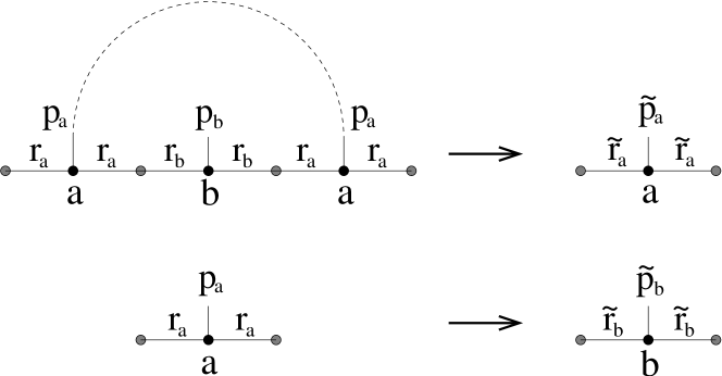
Figure 9: Renormalization scheme for the $k=2$ silver-mean network. Sites of the original network are symbolized by black circles while the additional sites by grey circles.

When in an arbitrary stadium of the renormalization procedure the parameters are $r_{a}$,$r_{b}$,$p_{a}$ and $p_{b}$ then, after the next generation of long links is eliminated, the renormalized parameters can be expressed in terms of the original ones as

$$\tilde{r}_{a}=r_{a}+\frac{p_{a}(r_{a}+r_{b})}{p_{a}+r_{a}+r_{b}},\qquad\tilde{r}_{b}=r_{a},$$

$$\tilde{p}_{a}=p_{b}+\frac{(r_{a}+r_{b})^{2}}{2(p_{a}+r_{a}+r_{b})},\qquad\tilde{p}_{b}=p_{a}.$$ (15)

After a lengthy but elementary calculation one obtains that the ansatz $\tilde{r}_{a}/r_{a}=\tilde{r}_{b}/r_{b}=\tilde{p}_{a}/p_{a}=\tilde{p}_{b}/p_{b}\equiv\overline{\lambda}$ solves the above system of equations with the scaling factor $\overline{\lambda}=\frac{1}{1+\sqrt{2}}+\sqrt{2\sqrt{2}}$. The resistance exponent is thus $\zeta=\frac{\ln\overline{\lambda}}{\ln\lambda}=\ln\left(\frac{1}{1+\sqrt{2}}+\sqrt{2\sqrt{2}}\right)/\ln(1+\sqrt{2})$ and the random-walk dimension of the $k=2$ silver-mean network is $d_{\rm rw}=1+\zeta=\ln\left(1+\sqrt{4+2\sqrt{2}}\right)/\ln(1+\sqrt{2})\approx 1.4575$.

V Discussion

We have seen that, in the networks studied in this work, the distribution of edge lengths is broad and, as a consequence, the length of shortest paths grows sub-linearly with the distance and random walk becomes super-diffusive. A model similar to random networks of this class (although, not $n$-regular) is the model by Benjamini and Berger, where any pairs of sites in a distance $l$ are connected with probability $p_{l}\sim\beta l^{-s-1}$ for large $l$. In that model, the diameter $D$, which is measured in terms of chemical distances, was conjectured to grow with the system size as $D(N)\sim N^{d_{\rm min}(\beta)}$ with some $\beta$-dependent exponent $0<d_{\rm min}(\beta)<1$ in the marginal case $s=1$ bb . Later, a power-law lower bound for $\beta<1$ and a power-law upper bound for any $\beta$ were shown to exist asymptotically with high probability for the size dependence of the diameter coppersmith . Thus, as far as the length of shortest paths (or the diameter) is concerned, random networks studied in this paper behave as that model is conjectured to do. Furthermore, we have shown that beside $d_{\rm min}$, the random-walk dimension is also influenced by the details of the structure of networks in the marginal point $s=1$ levy .

By means of the class of networks introduced in this work, a different type of control of the diffusion exponent can be realized compared to previous models. The control parameter is not the index $s$ as in the Lévy flight, which is set to its marginal value $s=1$ here, nor the prefactor $\beta$ as in the marginal Benjamini-Berger model but the number $k$ and other possible parameters appearing in the construction procedure. The prefactor $\beta$ in the distribution of lengths, as well as the shortest-path dimension and the random-walk dimension of these networks are non-trivial functions of these parameters.

We have also shown that by a sequence of $k=1$ aperiodic networks, the normal diffusion limit ($d_{\rm rw}=2$) can be approached arbitrarily closely. According to numerical results for $k=1,2,3$ uniform networks, the random-walk dimension decreases with the parameter $k$ and if $k\to\infty$, the latter quantity tends presumably to the ballistic limit $d_{\rm rw}=1$.

As opposed to the diffusion exponent that varies continuously with the index $s$ in case of the Lévy flight, the set of possible values of $d_{\rm rw}$ which can be realized by these networks is discrete. Nevertheless, one can define uniform networks where the parameter $k$ is not fixed but more than one values of $k$ are used in the construction procedure, e.g. $k\in\{n,n+1\}$ with a fixed positive integer $n$. The random-walk dimension of such “mixed” networks is expected to interpolate between that of “pure” ones constructed with a single $k$.

In a sub-class of networks introduced in this paper, the dimensions $d_{\rm min}$ and $d_{\rm rw}$ have been calculated exactly; in some cases they have been estimated by numerical methods. The possible exact calculation of these dimensions for other networks of this class or finding rigorous bounds on these quantities is the task of future research.

Appendix A

Let us consider a network built on an open one-dimensional lattice of size $N$. Connect the sites at the ends of the lattice (site $1$ and $N$) with a directed link which the walker can traverse only in one direction, say from site $1$ to site $N$ with a unit rate. Let us denote the probability that the random walker can be found at site $i$ in the steady-state by $\pi_{i}$. These probabilities satisfy the set of linear equations

$$\sum_{j}w_{ij}(\pi_{i}-\pi_{j})=0,\quad 1<i<N,$$ (16)

where the summation goes over the set of sites connected with site $i$ and $w_{ij}$ denotes the jump rate from site $i$ to site $j$; in our case $w_{N1}=0$ and $w_{ij}=1$ for other pairs $(i,j)$ of connected sites. Now, one can notice that Eq. 16 is analogous to Kirchhoff’s first law for electric circuits. Namely, $\pi_{i}$ plays the role of the potential at site $i$ and $1/w_{ij}$ corresponds to the resistance of link $(i,j)$. Consequently, if the part of the network between site $1$ and $N$ (except of the directed link) is replaced with a single (symmetric) link with a jump rate $1/\tilde{r}$, where $\tilde{r}$ is the effective resistance of the equivalent resistor network, the steady-state current $J$ through the directed link remains unchanged. On the other hand, we may write for $J$ in this simplified “circuit”, which consists of site $1$ and site $N$, as well as the directed link and the effective symmetric link connecting them:

$$J=\pi_{1}=(\pi_{N}-\pi_{1})\tilde{r}^{-1}.$$ (17)

If $N\gg 1$, the effective resistance is also large and we have $J=\pi_{1}\approx\pi_{N}\tilde{r}^{-1}$. If all the links were symmetric, the walker would be distributed uniformly on the network in the steady state. Although the link between site $1$ and site $N$ is directed and this leads to that the network is depleted on the side containing site $1$, the steady-state probabilities far from the end $1$ such as $\pi_{N}$ are still proportional to $1/N$ for large $N$. The expected value of the time $t$ that the walker needs to make a complete tour on the network (from site $N$ to the same site through the directed link) is related to the current as $t=1/J$. Thus, it scales with the size of the network as $t\approx\pi_{N}^{-1}\tilde{r}\sim N^{1+\zeta}$ in the large $N$ limit, from which we arrive at Eq. (2).

References

- (1) S. Havlin and D. Ben-Avraham, Adv. Phys. 36, 695 (1987).
- (2) J.P. Bouchaud and A. Georges, Phys. Rep. 195, 217 (1990).
- (3) M.F. Shlesinger, B.J. West and J. Klafter, Phys. Rev. Lett. 58, 1100 (1987), and references therein.
- (4) T.H. Solomon, E.R. Weeks and H.L. Swinney, Phys. Rev. Lett. 71, 3975 (1993).
- (5) A. Ott, J.P. Bouchaud, D. Langevin and W. Urbach, Phys. Rev. Lett. 65, 2201 (1990).
- (6) B.D. Hughes, M.F. Shlesinger and E.W. Montroll, Proc. Natl. Acad. Sci. 78, 3287 (1981); M.F. Shlesinger, G.M. Zaslavsky and J. Klafter, Nature 363, 31 (1993).
- (7) D.J. Watts and S.H. Strogatz, Nature 393, 440 (1998).
- (8) M.E.J. Newman and D.J. Watts, Phys. Lett. A 263, 341 (1999).
- (9) C.F. Moukarzel, Phys. Rev. E 60, R6263 (1999).
- (10) R. Monasson, Eur. Phys. J. B 12, 555 (1999).
- (11) S. Jespersen and A. Blumen, Phys. Rev. E 62, 6270 (2000).
- (12) I. Benjamini and N. Berger, Rand. Struct. Alg. 19, 102 (2001).
- (13) P. Sen and B. Chakrabarti, J. Phys. A: Math. Gen. 34, 7749 (2001).
- (14) C.F. Moukarzel and M. Argollo de Menezes, Phys. Rev. E 65, 056709 (2002).
- (15) D. Coppersmith, D. Gamarnik and M. Sviridenko, Rand. Struct. Alg. 21, 1 (2002).
- (16) J.M. Kleinberg, Nature 406, 845 (2000).
- (17) I. Benjamini and C. Hoffman, Electr. J. Comb., 12, R46 (2005).
- (18) S. Boettcher, B. Gonçalves and H. Guclu, J. Phys. A: Math. Theor. 41, 252001 (2008); S. Boettcher and B. Gonçalves, preprint, arXiv:0802.2757.
- (19) Y. Gefen, A. Aharony and S. Alexander, Phys. Rev. Lett. 50, 77 (1983).
- (20) Y. Gefen and I. Goldhirsch, Phys. Rev. B 35, 8639 (1987).
- (21) K. Hida, Phys. Rev. Lett. 93, 037205 (2004); A.P. Vieira, Phys. Rev. B 71, 134408 (2005).
- (22) R. Juhász and Z. Zimborás, J. Stat. Mech. P04004 (2007).
- (23) A.J. Bray, B. Derrida and C. Godrèche, Europhys. Lett. 27, 175 (1994).
- (24) D.S. Fisher, Phys. Rev. B 50, 3799 (1994).
- (25) Note that the typical displacement in symmetric Lévy flights with a jump length distribution of the form increases with the time as .