UTHEP-563 RIKEN-TH-130 May 2008

D-brane States and Annulus Amplitudes in

$OSp$ Invariant Closed String Field Theory

Yutaka Baba^a, Nobuyuki Ishibashi^b, Koichi Murakami^a

^aTheoretical Physics Laboratory, RIKEN,
Wako, Saitama 351-0198, Japan

^bInstitute of Physics, University of Tsukuba,
Tsukuba, Ibaraki 305-8571, Japan

In the $OSp$ invariant closed string field theory, we construct the states corresponding to parallel D-branes that are located at different points in the space-time. Using these states, we evaluate annulus amplitudes. We show that the results coincide with those of first quantized string theory.

1 Introduction

D-branes have been playing an important role in understanding nonperturbative aspects of string theory. In previous works [1][2], we studied how to describe D-branes in closed string field theory. The closed string field theory that we consider is the $OSp$ invariant string field theory for bosonic strings [3]. (See also [4][5][6][7].) We constructed the states with an arbitrary number of coincident D-branes and ghost D-branes [8] in this closed string field theory. We can calculate disk amplitudes using these states, and the results coincide with those of first quantized string theory [2].

In this paper, we extend our construction into the case where the D-branes are located at different points from each other in the space-time. Using such a state with two D-branes, we evaluate annulus amplitudes. We show that they coincide with the usual annulus amplitudes including the normalizations. This fact yields another evidence for our construction.

The organization of this paper is as follows. In section 2, we generalize our previous construction [2] to propose the states for $N$ parallel D$p$-branes that are located at different points from each other. We show that these states are BRST invariant in the leading order in the regularization parameter $\epsilon$. In section 3, we compute annulus amplitudes and show that the results in first quantized string theory are reproduced. Section 4 is devoted to conclusions. In appendix A, we present details of the calculation.

2 States with Parallel D-branes at Different Points

The BRST invariant state corresponding to one flat D$p$-brane sitting at $X^{i}=Y^{i}$ $(i=p+1,\ldots,25)$ is constructed in [2] as

$$|D_{+}(Y)\rangle\!\rangle=\lambda\left(\int d\zeta\bar{\mathcal{O}}_{D}\left(\zeta,Y\right)\right)|0\rangle\!\rangle~{},$$ (2.1)

where

$$\bar{\mathcal{O}}_{D}(\zeta,Y)=\exp\left[A\int^{0}_{-\infty}dr\,\frac{e^{\zeta\alpha_{r}}}{\alpha_{r}}\,{}^{\epsilon}_{r}\langle B_{0}(Y)|\bar{\psi}\rangle_{r}+B\zeta^{2}\right]~{},$$

$$\qquad A=\frac{(2\pi)^{13}}{(8\pi^{2})^{\frac{p+1}{2}}\sqrt{\pi}}~{},\quad B=\frac{(2\pi)^{13}\epsilon^{2}(-\ln\epsilon)^{\frac{p+1}{2}}}{16\left(\frac{\pi}{2}\right)^{\frac{p+1}{2}}\sqrt{\pi}g}~{}.$$ (2.2)

Here $|B_{0}(Y)\rangle\equiv e^{-ip_{i}Y^{i}}|B_{0}\rangle$ denotes the boundary state for the D$p$-brane located at $X^{i}=Y^{i}$ and $|B_{0}\rangle=|B_{0}(0)\rangle$ is given in [2]. As in [2], we introduce the state

$$|B_{0}(Y)\rangle^{T}=e^{-\frac{T}{|\alpha|}(L_{0}+\tilde{L}_{0}-2)}|B_{0}(Y)\rangle~{},$$ (2.3)

and use $|B_{0}(Y)\rangle^{\epsilon}$ with $0<\epsilon\ll 1$ as a regularized version of $|B_{0}(Y)\rangle$. $\int d\zeta\bar{\mathcal{O}}_{D}$ can be considered as an operator which creates the D-brane by acting on the second quantized vacuum $|0\rangle\!\rangle$. With string field $|\bar{\psi}\rangle$ exponentiated, this operator has the effect of inserting boundaries in the worldsheet.

We would like to show that the states corresponding to $N$ such D$p$-branes located at $X^{i}=Y^{i}_{(I)}$ $(I=1,\ldots,N)$ can be given simply as

$$|D_{N+};Y_{(I)}\rangle\!\rangle=\lambda_{N+}\prod_{I=1}^{N}\left(\int d\zeta_{I}\bar{\mathcal{O}}_{D}\left(\zeta_{I},Y_{(I)}\right)\right)|0\rangle\!\rangle~{},$$ (2.4)

if $(Y^{i}_{(I)}-Y^{i}_{(J)})^{2}\neq 0$ for $I\neq J$. In contrast to the case of coincident D-branes studied in [2], we just have to consider the product of $\int d\zeta\bar{\mathcal{O}}_{D}$. Indeed, we can show that as long as $(Y^{i}_{(I)}-Y^{i}_{(J)})^{2}\neq 0$ for $I\neq J$, the states (2.4) are BRST invariant in the leading order in the regularization parameter $\epsilon$. The proof goes exactly as in [2]. One crucial difference from the coincident case is that in the limit of $T=\epsilon\rightarrow 0$ the string vertex

$$\langle V_{1}(3);Y,Y^{\prime};T|\equiv\int d^{\prime}1d^{\prime}2\,\langle V_{3}(1,2,3)|B_{0}(Y)\rangle^{T}_{1}|B_{0}(Y^{\prime})\rangle^{T}_{2}$$ (2.5)

is suppressed by $\epsilon^{\frac{(\Delta Y^{i})^{2}}{4\pi^{2}}}$ with $\Delta Y^{i}\equiv Y^{i}-Y^{\prime i}$, compared with $\langle V_{1}(3);T|$ evaluated in [2]. Because of this suppression, the interaction between $\bar{\mathcal{O}}_{D}$ at different points can be ignored in the leading order in $\epsilon$ and the states (2.4) become BRST invariant.

The details of the calculation of $\langle V_{1}(3);Y,Y^{\prime};T|$ are presented in appendix A. The suppression stated above is intuitively obvious, because the D-branes sit at different points. The suppression factor originates from the factor $e^{-S_{\mathrm{cl}}}$, where $S_{\mathrm{cl}}$ is the classical action given in eq.(A.11) on the worldsheet depicted in Fig. 3 in appendix A. Indeed, using the results in [9][10][2], we find that in the $T=\epsilon\rightarrow 0$ limit

$$e^{-S_{\mathrm{cl}}}\sim\left(\frac{\epsilon}{4\alpha\sin(-2\pi V_{3})}\right)^{\frac{(\Delta Y^{i})^{2}}{4\pi^{2}}}~{}.$$ (2.6)

In addition to the BRST invariance mentioned above, it is easy to see that using the states (2.4) one can calculate the disk amplitudes in the same way as in [2] and obtain those for the parallel D-branes. Thus we may regard the states (2.4) as the ones where such D-branes exist. We can also generalize the states (2.4) to include ghost D-branes [8], as is carried out in [2].

3 Annulus Amplitudes Derived from D-brane States

3.1 Amplitudes with one closed string external line

Using the states with D-branes constructed in the last section, we would like to calculate scattering amplitudes involving the strings whose worldsheets have boundaries attached to D-branes contained in these states. In this paper, we evaluate annulus amplitudes. Let us first consider the annulus amplitudes with one closed string external line as described in Fig. 1 (a), in the situation where the annulus is suspended between two parallel D$p$-branes located at $X^{i}=Y^{i}$ and $Y^{\prime i}$.

Figure 1: (a) The annulus diagram with one closed string external state $\phi$. (b) The $\tilde{\nu}$ coordinate on the worldsheet of the string diagram in (a). At $\tilde{\nu}=i\pi\tilde{\tau}\varrho$, the vertex operator $V_{\phi}$ corresponding to the state $\phi$ is inserted.

The S-matrix element for this process can be obtained from the following correlation function involving these two D$p$-branes:

$$\left\langle\!\left\langle\mathcal{O}_{\phi}(t,k)\right\rangle\!\right\rangle_{D_{2+}(Y;Y^{\prime})}\equiv\frac{\langle\!\langle 0|\mathcal{O}_{\phi}(t,k)|D_{2+};Y,Y^{\prime}\rangle\!\rangle}{\langle\!\langle 0|D_{2+};Y,Y^{\prime}\rangle\!\rangle}~{},$$ (3.1)

where $t>0$. $\mathcal{O}_{\phi}(t,k)$ is the observable corresponding to the external state $\phi$ defined [11] as

$$\mathcal{O}_{\phi}(t,k)=\int dr\,\frac{1}{\alpha_{r}}\,{}_{r}\Big{(}{}_{C,\bar{C}}\langle 0|\otimes{}_{X}\langle\mbox{primary}_{\phi};k|\Big{)}|\Phi(t)\rangle_{r}~{},$$ (3.2)

where $|\mbox{primary}_{\phi};k\rangle_{X}$ is a normalized Virasoro primary state with momentum $k$, corresponding to a particle with mass $M$. In the correlation function (3.1) we should evaluate the contribution $G_{\phi DD^{\prime}}(k)$ from the annulus diagram suspended between the two D$p$-branes contained in $|D_{2+};Y,Y^{\prime}\rangle\!\rangle$. This is an order $\mathcal{O}(g)$ term in the correlation function (3.1).

Perturbatively, for the $\zeta_{I}$ $(I=1,2)$ integrations in eq.(2.4) the saddle point method becomes a good approximation [1][2] and yields

$$\left|\left.D_{2+};Y,Y^{\prime}\right\rangle\!\right\rangle\simeq\lambda^{\prime}\exp\left[A\int^{0}_{-\infty}\frac{dr_{1}}{\alpha_{r_{1}}}\,{}_{r_{1}}^{\epsilon}\langle B_{0}(Y)|\bar{\psi}\rangle_{r_{1}}\right]\exp\left[A\int^{0}_{-\infty}\frac{dr_{2}}{\alpha_{r_{2}}}\,{}_{r_{2}}^{\epsilon}\langle B_{0}(Y^{\prime})|\bar{\psi}\rangle_{r_{2}}\right]|0\rangle\!\rangle~{},$$ (3.3)

where $\lambda^{\prime}=-\frac{\pi}{B}\lambda_{2+}$. Using these, we obtain

$$G_{\phi DD^{\prime}}(k)=-3!A^{2}\int^{\infty}_{0}\frac{d1}{\alpha_{1}}\int^{\infty}_{0}\frac{d2}{\alpha_{2}}\int^{0}_{-\infty}\frac{d3}{\alpha_{3}}\int^{t}_{0}dT\,\frac{2g}{3}\langle V_{3}^{0}(1,2,3)|$$ (3.4)

$$\hskip 50.00008pt\times|B_{0}(Y)\rangle_{1}^{T}|B_{0}(Y^{\prime})\rangle_{2}^{T}\,e^{\frac{t-T}{\alpha_{3}}(L^{(3)}_{0}+\tilde{L}^{(3)}_{0}-2)}\Big{(}|\mbox{primary}_{\phi};k\rangle_{X}\otimes|0\rangle_{C,\bar{C}}\Big{)}_{3}~{},$$

where $T$ corresponds to the proper time of the three-string interaction vertex. We have performed the Wick rotation so as to make the proper time Euclidean. Using eqs.(A.2) and (A.4), the right hand side of eq.(3.4) can be rewritten as

$$G_{\phi DD^{\prime}}(k)=-gA^{2}\int_{0}^{\infty}d\alpha\int^{\alpha}_{0}d\alpha_{1}\int^{t}_{0}dT\int\frac{d^{26}p_{3}}{(2\pi)^{26}}id\bar{\pi}_{0}^{(3)}d\pi_{0}^{(3)}\,\mathcal{K}_{1}(3;Y,Y^{\prime};T)$$ (3.5)

$$\times(2\pi)^{p+1}\delta_{\mathrm{N}}^{p+1}(p_{3})\langle V^{0}_{1,\mathrm{LPP}}(3);Y,Y^{\prime};T|e^{-\frac{t-T}{\alpha}(L^{(3)}_{0}+\tilde{L}^{(3)}_{0}-2)}\Bigl{(}|\mbox{primary}_{\phi};k\rangle_{X}\otimes|0\rangle_{C,\bar{C}}\Bigr{)}_{3},~{}~{}~{}$$

where $\alpha=-\alpha_{3}$, $\mathcal{K}_{1}(3;Y,Y^{\prime};T)$ is a factor given in eq.(A.12) and $\delta^{p+1}_{\mathrm{N}}(p_{3})$ denotes the delta function of the momentum in the directions along the D$p$-branes. In the following, we would like to rewrite the right hand side of eq.(3.5) into a form which can be compared with the usual annulus amplitude.

LPP vertex $\langle V^{0}_{1,\mathrm{LPP}}(3);Y,Y^{\prime};T|$

$\langle V^{0}_{1,\mathrm{LPP}}(3);Y,Y^{\prime};T|$ can be expressed as a direct product of a state in the $C,\bar{C}$ Fock space and one in the $X$ Fock space, namely

$${}_{C,\bar{C}}\langle V^{0}_{1,\mathrm{LPP}}(3);Y,Y^{\prime};T|\otimes{}_{X}\langle V^{0}_{1,\mathrm{LPP}}(3);Y,Y^{\prime};T|~{}.$$ (3.6)

Since ${}_{C,\bar{C}}\langle V^{0}_{1,\mathrm{LPP}}(3);Y,Y^{\prime};T|$ has the form

$${}_{C,\bar{C}}\langle V^{0}_{1,\mathrm{LPP}}(3);Y,Y^{\prime};T|={}_{C,\bar{C}}\langle 0|e^{-\frac{T}{\alpha}2i\pi_{0}^{(3)}\bar{\pi}_{0}^{(3)}+\mbox{\footnotesize{ (terms quadratic or linear in oscillators)} }}~{},$$ (3.7)

the contribution from the $C,\bar{C}$ sector to $G_{\phi DD^{\prime}}(k)$ in eq.(3.5) becomes

$$\int id\bar{\pi}_{0}^{(3)}d\pi_{0}^{(3)}{}_{C,\bar{C}}\langle V^{0}_{1,\mathrm{LPP}}(3);Y,Y^{\prime};T|0\rangle_{C,\bar{C}}\,e^{-\frac{t-T}{\alpha}2i\pi_{0}^{(3)}\bar{\pi}_{0}^{(3)}}=\frac{2t}{\alpha}~{}.$$ (3.8)

From the definition of the LPP vertex [12], one can see that the overlap

$$\int\frac{d^{26}p_{3}}{(2\pi)^{26}}(2\pi)^{p+1}\delta_{\mathrm{N}}^{p+1}(p_{3}){}_{X}\langle V^{0}_{1,\mathrm{LPP}}(3);Y,Y^{\prime};T|\mbox{primary}_{\phi};k\rangle_{X,3}~{}$$ (3.9)

is written in terms of a correlation function on the annulus. In order to express the correlation function using the boundary states, it is convenient to use the worldsheet coordinate $\tilde{\nu}$ depicted in Fig. 1 (b), which is related to the coordinate $\nu$ in Fig. 3 (b) by

$$\tilde{\nu}=\frac{2\pi}{-i\tau}\nu~{}.$$ (3.10)

In this coordinate, the annulus diagram in Fig. 1 (a) is described as a cylinder of circumference $2\pi$. The length of the cylinder is $-i\pi\tilde{\tau}$ and the vertex operator corresponding to the external state is inserted at

$$\tilde{\nu}=\frac{2\pi}{-i\tau}V_{3}=i\pi\tilde{\tau}\varrho~{},$$ (3.11)

where

$$\tilde{\tau}=-\frac{1}{\tau}~{},\qquad\varrho=-2V_{3}=\frac{\alpha_{1}}{\alpha}~{}.$$ (3.12)

The overlap (3.9) can be written as a correlation function on the cylinder with the coordinate $\tilde{\nu}$ as follows:

$$\int\frac{d^{26}p_{3}}{(2\pi)^{26}}(2\pi)^{p+1}\delta_{\mathrm{N}}^{p+1}(p_{3}){}_{X}\langle V^{0}_{1,\mathrm{LPP}}(3);Y,Y^{\prime};T|\mbox{primary}_{\phi};k\rangle_{X,3}$$ (3.13)

$$\quad=N(\tilde{\tau})\left|\frac{\partial w_{3}}{\partial\tilde{\nu}}(i\pi\tilde{\tau}\varrho)\right|^{-\left(k^{2}+M^{2}+2\right)}$$

$$\quad\qquad\times{}_{X}\langle B_{0}(Y^{\prime})|e^{i\pi\tilde{\tau}\varrho\left(L_{0}^{X}+\tilde{L}_{0}^{X}-2\right)}\,V_{\phi}\,e^{i\pi\tilde{\tau}(1-\varrho)\left(L_{0}^{X}+\tilde{L}_{0}^{X}-2\right)}|B_{0}(Y)\rangle_{X}~{}.$$

Here $L^{X}_{0}$ and $\tilde{L}_{0}^{X}$ are the zero-modes of the Virasoro generators and $|B_{0}(Y)\rangle_{X}$ is the boundary state in the $X$ sector given in [2]. $V_{\phi}$ denotes the vertex operator of weight $(\frac{1}{2}(k^{2}+M^{2}+2),\frac{1}{2}(k^{2}+M^{2}+2))$ corresponding to the state $|\mbox{primary}_{\phi};k\rangle_{X}$. $N(\tilde{\tau})$ is a normalization factor independent of $\phi$, which can be fixed by considering the case $V_{\phi}=1$, and we obtain

$$N(\tilde{\tau})=\eta(\tilde{\tau})^{24}\prod_{n=1}^{\infty}\left(1-e^{2\pi i\tilde{\tau}n}\right)^{2}e^{S_{\mathrm{cl}}}(2\pi)^{26-(p+1)}(-i\tilde{\tau})^{13-\frac{p+1}{2}}~{}.$$ (3.14)

By using eqs.(3.10), (A.3) and (A.6), we also obtain

$$\frac{\partial w_{3}}{\partial\tilde{\nu}}(i\pi\tilde{\tau}\varrho)=\frac{-i\tau}{2\pi}\left.\frac{\partial w_{3}}{\partial\nu}\right|_{\nu=V_{3}}=-i\tau\frac{\eta(\tau)^{3}}{\vartheta_{1}(2V_{3}|\tau)}e^{\frac{T}{\alpha}}~{}.$$ (3.15)

Integration measure

In eq.(3.5), we should change the integration variables $(\alpha_{1},T)$ to $(\varrho,\tilde{\tau})$. For a fixed $\alpha$, eq.(3.12) implies that

$$d\alpha_{1}=\alpha d\varrho~{},\qquad dT=\frac{\partial T}{\partial\tilde{\tau}}d\tilde{\tau}=\frac{\partial T}{\partial\tau}\frac{1}{\tilde{\tau}^{2}}d\tilde{\tau}~{}.$$ (3.16)

We find that $\partial T/\partial\tau$ becomes

$$\frac{\partial T}{\partial\tau}=-\frac{i}{4\pi}c_{I}~{},$$ (3.17)

where $c_{I}$ is given in eq.(A.13). This can be derived from eqs.(A.6), (A.7) and (A.13) as follows:

$$\frac{\partial T}{\partial\tau} = \frac{\partial\rho}{\partial\nu}(\nu_{I}^{-})\,\frac{\partial\nu_{I}^{-}}{\partial\tau}+\left.\alpha\frac{\partial}{\partial\tau}\ln\frac{\vartheta_{1}(\nu+V_{3}|\tau)}{\vartheta_{1}(\nu-V_{3}|\tau)}\right|_{\nu=\nu_{I}^{-}}=\left.\alpha\frac{\partial}{\partial\tau}\ln\frac{\vartheta_{1}(\nu+V_{3}|\tau)}{\vartheta_{1}(\nu-V_{3}|\tau)}\right|_{\nu=\nu_{I}^{-}}$$ (3.18)

$$= -\frac{i}{4\pi}\alpha\left[\frac{\partial^{2}_{\nu}\vartheta_{1}(\nu^{-}_{I}+V_{3}|\tau)}{\vartheta_{1}(\nu^{-}_{I}+V_{3}|\tau)}-\frac{\partial^{2}_{\nu}\vartheta_{1}(\nu^{-}_{I}-V_{3}|\tau)}{\vartheta_{1}(\nu^{-}_{I}-V_{3}|\tau)}\right]=-\frac{i}{4\pi}c_{I}~{}.$$

Here we have used the fact that the theta function $\vartheta_{1}(\nu|\tau)$ satisfies the heat equation,

$$\frac{\partial}{\partial\tau}\vartheta_{1}(\nu|\tau)=-\frac{i}{4\pi}\frac{\partial^{2}}{\partial\nu^{2}}\vartheta_{1}(\nu|\tau)~{}.$$ (3.19)

S-matrix element

Collecting all these results, we can obtain

$$G_{\phi DD^{\prime}}(k)=-4\pi^{2}gA^{2}\int^{\infty}_{0}d\alpha\,\frac{t}{\alpha^{2}}\,e^{-\frac{t}{\alpha}(k^{2}+M^{2})}\int^{1}_{0}d\varrho\int^{\tilde{\tau}_{0}(\alpha,\varrho)}_{0}d\tilde{\tau}\,\tilde{\tau}\left|\frac{e^{-i\pi\varrho^{2}\tilde{\tau}}\eta(\tilde{\tau})^{3}}{\vartheta_{1}(\varrho\tilde{\tau}|\tilde{\tau})}\right|^{-(k^{2}+M^{2})}$$ (3.20)

$$\ \quad\times\prod_{n=1}^{\infty}\left(1-e^{2\pi in\tilde{\tau}}\right)^{2}{}_{X}\langle B_{0}(Y^{\prime})|e^{i\pi\tilde{\tau}\varrho(L_{0}^{X}+\tilde{L}_{0}^{X}-2)}\,V_{\phi}\,e^{i\pi\tilde{\tau}(1-\varrho)(L_{0}^{X}+\tilde{L}_{0}^{X}-2)}|B_{0}(Y)\rangle_{X}~{},~{}~{}~{}$$

where $\tilde{\tau}_{0}(\alpha,\varrho)$ is the value of $\tilde{\tau}(=\tilde{\tau}(T,\alpha,\varrho))$ when $T=t$: $\tilde{\tau}_{0}(\alpha,\varrho)=\tilde{\tau}(t,\alpha,\varrho)$.

In order to obtain the S-matrix element $S_{\phi DD^{\prime}}$ for the process we are considering, we need look for the singular behavior of $G_{\phi DD^{\prime}}(k)$ near the mass-shell of the external state, namely $k^{2}+M^{2}\sim 0$. As explained in [11], such singularity comes from the region $\alpha\sim 0$ in the integration over $\alpha$, and we find

$$G_{\phi DD^{\prime}}(k) \sim -4\pi^{2}gA^{2}\frac{1}{k^{2}+M^{2}}\int^{1}_{0}d\varrho\int^{i\infty}_{0}d\tilde{\tau}\,\tilde{\tau}\,\prod_{n=1}^{\infty}\left(1-e^{2\pi in\tilde{\tau}}\right)^{2}$$ (3.21)

$$\ \times{}_{X}\langle B_{0}(Y^{\prime})|e^{i\pi\tilde{\tau}\varrho(L_{0}^{X}+\tilde{L}_{0}^{X}-2)}\,V_{\phi}\,e^{i\pi\tilde{\tau}(1-\varrho)(L_{0}^{X}+\tilde{L}_{0}^{X}-2)}|B_{0}(Y)\rangle_{X}~{}.$$

Here we have used the relation

$$\lim_{\alpha\rightarrow 0}\tilde{\tau}_{0}(\alpha,\varrho)=i\infty~{}.$$ (3.22)

Thus we obtain the S-matrix element $S_{\phi DD^{\prime}}$,

$$S_{\phi DD^{\prime}}(k) = -4\pi^{2}igA^{2}\int^{1}_{0}d\varrho\int^{i\infty}_{0}d\tilde{\tau}\,\tilde{\tau}\,\prod_{n=1}^{\infty}\left(1-e^{2\pi in\tilde{\tau}}\right)^{2}$$ (3.23)

$$\ \times{}_{X}\langle B_{0}(Y^{\prime})|e^{i\pi\tilde{\tau}\varrho(L_{0}^{X}+\tilde{L}_{0}^{X}-2)}\,V_{\phi}\,e^{i\pi\tilde{\tau}(1-\varrho)(L_{0}^{X}+\tilde{L}_{0}^{X}-2)}|B_{0}(Y)\rangle_{X}~{},$$

where the momentum $k_{\hat{\mu}}$ $(\hat{\mu}=0,\ldots,25)$ of the vertex operator $V_{\phi}$ is subject to the on-shell condition: $k^{2}+M^{2}=0$. Here we have performed the Wick rotation to make the space-time signature Lorentzian.

In this form, it is obvious that $S_{\phi DD^{\prime}}$ is proportional to the S-matrix element in first quantized string theory. The factor $\prod_{n=1}^{\infty}\left(1-e^{2\pi in\tilde{\tau}}\right)^{2}$ coincides with the ghost contribution to the partition function. As is described in Fig. 1 (b), the worldsheet of the process we are considering is a one-punctured cylinder. In eq.(3.23), the S-matrix element $S_{\phi DD^{\prime}}$ is expressed as an integral over the moduli space of the one-punctured cylinder with the correct integration measure $\tilde{\tau}d\tilde{\tau}d\varrho$. We notice that in this integral the moduli space is covered completely and only once.

3.2 Factorization of S-matrix element

Let us check that the S-matrix element in eq.(3.23) has the correct normalization. This can be done by considering the S-matrix element $S_{\phi DD^{\prime}}$ in the simplest case where $V_{\phi}$ corresponds to the tachyon:

$$V_{\phi}=\mbox{\tiny$\stackrel{{\scriptstyle\circ}}{{\scriptstyle\circ}}$}\,e^{ik\cdot X}\,\mbox{\tiny$\stackrel{{\scriptstyle\circ}}{{\scriptstyle\circ}}$}~{}.$$ (3.24)

Here $\stackrel{{\scriptstyle\circ}}{{\scriptstyle\circ}}$  $\stackrel{{\scriptstyle\circ}}{{\scriptstyle\circ}}$ denotes the normal ordering of the oscillators. We examine the behavior of $S_{\phi DD^{\prime}}$ at the poles from the tachyons of the closed strings exchanged between the two D-branes in Fig. 1 (a). This corresponds to the scattering process sketched in Fig. 2.

Figure 2: The scattering process near the poles from the tachyons of the closed strings exchanged between the two D-branes in Fig. 1 (a). The three solid lines connecting with each other indicate tachyon propagations.

In order to obtain the singular behaviour, we perform the Fourier transformation of the S-matrix element $S_{\phi DD^{\prime}}$ with respect to $Y^{i}$ and $Y^{\prime i}$, and then put the conjugate momenta $k_{1}$ and $k_{2}$ close to the mass-shell of the tachyon. In the region where $k_{1}^{2}\sim 2$ and $k_{2}^{2}\sim 2$, $S_{\phi DD^{\prime}}$ becomes

$$S_{\phi DD^{\prime}}\sim\int\frac{d^{26}k_{1}}{(2\pi)^{26}}\int\frac{d^{26}k_{2}}{(2\pi)^{26}}S_{TD}(-k_{1};Y)\frac{-i}{k_{1}^{2}-2}S_{TTT}(k,k_{1},k_{2})\frac{-i}{k_{2}^{2}-2}S_{TD}(-k_{2};Y^{\prime})~{},$$ (3.25)

where

$$S_{TTT}(k,k_{1},k_{2}) = i4g(2\pi)^{26}\delta^{26}(k+k_{1}+k_{2})~{},$$

$$S_{TD}(k_{1};Y) = iA(2\pi)^{p+1}\delta^{p+1}_{\mathrm{N}}(k_{1})e^{ik_{1,i}Y^{i}}~{}.$$ (3.26)

In this equation, $S_{TTT}(k,k_{1},k_{2})$ is the tree amplitude for three closed string tachyons with momenta $k$, $k_{1}$ and $k_{2}$, and $S_{TD}(k_{1};Y)$ is the coupling of the D$p$-brane located at $X^{i}=Y^{i}$ to a closed string tachyon with momentum $k_{1}$. Eq.(3.25), therefore, implies that the factorization occurs in the right way in $S_{\phi DD^{\prime}}$ and thus $S_{\phi DD^{\prime}}$ has the correct normalization.

3.3 More general amplitudes

It is easy to generalize the calculation above and consider more general annulus amplitudes. For example, let us consider the amplitudes with the annulus ending on the same D-brane. In this case the computations are the same as those in the case of two D-branes, except that this time the S-matrix elements are deduced from the contributions of the term quadratic in the boundary state contained only in a single $\bar{\mathcal{O}}_{D}$. Therefore the normalizations of the S-matrix elements become half of those in the case of two D-branes. Thus we obtain the correct normalizations.

We can also calculate the annulus amplitudes with any number of closed string insertions. We can compute such amplitudes by using the fact that the three-string interaction vertex overlapped by an external state reduces to the vertex operator for the state, when the external state is close to the mass-shell [2]. Therefore the computation comes down to the one we have done above. It is easy to check that the resulting S-matrix elements are expressed as an integral over the moduli space with the appropriate measure and have the correct normalizations.

4 Conclusions

In this paper, we construct states corresponding to $N$ parallel D$p$-branes located separately from each other. We show that these states are BRST invariant in the leading order in $\epsilon$. Using these states, we can calculate annulus amplitudes. We show that usual annulus amplitudes are reproduced. The analyses in this paper provide another evidence for our construction of the D-brane states in the $OSp$ invariant closed string field theory.

Appendix A Details of Calculation of $\langle V_{1}(3);Y,Y^{\prime};T|$

In this appendix, we present details of the calculation of the string vertex (2.5).

The vertex (2.5) is expressed as

$$\langle V_{1}(3);Y,Y^{\prime};T|=\langle V_{1}^{0}(3);Y,Y^{\prime};T|C(\rho_{I})\mathcal{P}_{3}~{},$$ (A.1)

where

$$\langle V^{0}_{1}(3);Y,Y^{\prime};T|\equiv\int d^{\prime}1\,d^{\prime}2\,\delta(1,2,3)\frac{|\mu(1,2,3)|^{2}}{\alpha_{1}\alpha_{2}\alpha_{3}}{}_{123}\langle 0|e^{E(1,2,3)}|B_{0}(Y)\rangle^{T}_{1}|B_{0}(Y^{\prime})\rangle^{T}_{2}~{}.$$ (A.2)

As carried out in [2], we introduce the complex coordinate $\rho$ on the worldsheet for the string diagram corresponding to the vertex (A.2) depicted in Fig. 3 (a). $\rho_{I}$ in eq.(A.1) denotes the interaction point on the $\rho$-plane. The external closed string corresponds to the string $3$. The region of the worldsheet corresponding to the propagation of this string is $|w_{3}|\leq 1$, where

$$\rho=\alpha_{3}\ln w_{3}+T~{}.$$ (A.3)

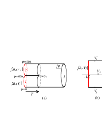
Figure 3: (a) The worldsheet for the string diagram corresponding to the vertex (A.2). The coordinate $\rho$ ($\mathrm{Re}\,\rho\geq 0$, $-\pi\alpha\leq\mathrm{Im}\,\rho\leq\pi\alpha$) is introduced on this worldsheet. (b) The rectangle on the $\nu$-plane related to the worldsheet in (a) by the Mandelstam mapping (A.6).

The vertex $\langle V_{1}^{0}(3);Y,Y^{\prime};T|$ takes the form

$$\langle V^{0}_{1}(3);Y,Y^{\prime};T| = 2\delta(\alpha_{1}+\alpha_{2}+\alpha_{3})(2\pi)^{p+1}\delta^{p+1}_{\mathrm{N}}(p_{3})$$ (A.4)

$$\quad\times\mathcal{K}_{1}(3;Y,Y^{\prime};T)\langle V^{0}_{1,\mathrm{LPP}}(3);Y,Y^{\prime};T|~{},$$

where $\mathcal{K}_{1}(3;Y,Y^{\prime};T)$ is the partition function of the CFT on the $\rho$-plane endowed with the metric $ds^{2}=d\rho d\bar{\rho}$ [13]. $\langle V^{0}_{1,\mathrm{LPP}}(3);Y,Y^{\prime};T|$ is the LPP vertex [12] of the form

$$\langle V^{0}_{1,\mathrm{LPP}}(3);Y,Y^{\prime};T|={}_{3}\langle 0|e^{E(3)}~{},$$ (A.5)

where $E(3)$ consists of terms linear or quadratic in $\alpha_{n}^{M(3)}$ and $\tilde{\alpha}_{n}^{M(3)}$ ($n\geq 0$).

Mandelstam mapping

In order to evaluate the string vertex (2.5), we use the Mandelstam mapping introduced in [2],

$$\rho(\nu)=\alpha\ln\frac{\vartheta_{1}(\nu+V_{3}|\tau)}{\vartheta_{1}(\nu-V_{3}|\tau)}~{},$$ (A.6)

where $\alpha\equiv\alpha_{1}+\alpha_{2}=-\alpha_{3}$, $V_{3}=-\frac{\alpha_{1}}{2\alpha}$ and $\vartheta_{1}(\nu|\tau)$ is a Jacobi theta function. This is the mapping between the $\rho$-plane and the rectangle on the complex $\nu$-plane defined by $-\frac{1}{2}\leq\mathrm{Re}\,\nu\leq 0$ and $-\frac{\tau_{2}}{2}\leq\mathrm{Im}\,\nu\leq\frac{\tau_{2}}{2}$ (Fig. 3 (b)). Here $\tau=i\tau_{2}$ ($\tau_{2}\in\mathbb{R}$, $\tau_{2}\geq 0$) is the modulus of the annulus and the identification $\nu\cong\nu+\tau$ should be made. The interaction points $\nu_{I}^{\pm}$ on the $\nu$-plane and the modulus $T$ on the $\rho$-plane satisfy

$$\frac{d\rho}{d\nu}(\nu_{I}^{\pm})=0~{},\quad T=\mathrm{Re}\rho(\nu_{I}^{-})=\rho(\nu_{I}^{-})+2\pi i\alpha V_{3}~{}.$$ (A.7)

Partition function $\mathcal{K}_{1}(3;Y,Y^{\prime};T)$

From the Mandelstam mapping (A.6), one can find that the boundary conditions imposed on the worldsheet variables $X^{i}(\nu,\bar{\nu})$ $(i=p+1,\ldots,25)$ on the $\nu$-plane are

$$\left.X^{i}(\nu,\bar{\nu})\right|_{\mathrm{Re}\,\nu=-\frac{1}{2}}=Y^{i}~{},\quad\left.X^{i}(\nu,\bar{\nu})\right|_{\mathrm{Re}\,\nu=0}=Y^{\prime i}~{},\quad X^{i}(\nu+\tau,\bar{\nu}+\bar{\tau})=X^{i}(\nu,\bar{\nu})~{},$$ (A.8)

and the other worldsheet variables $X^{\mu}(\nu,\bar{\nu})$ $(\mu=26,1,\ldots,p)$, $C(\nu,\bar{\nu})$ and $\bar{C}(\nu,\bar{\nu})$ obey the same boundary conditions as those in the case considered in [2]. Therefore, the classical configurations $X_{\mathrm{cl}}^{N}(\nu,\bar{\nu})$ for the worldsheet variables around which the quantum fluctuations $\tilde{X}^{N}(\nu,\bar{\nu})$ should be considered are

$$X^{i}_{\mathrm{cl}}(\nu,\bar{\nu})=Y^{\prime i}-(\nu+\bar{\nu})\Delta Y^{i}~{},\quad X^{\mu}_{\mathrm{cl}}(\nu,\bar{\nu})=0~{},\quad C_{\mathrm{cl}}(\nu,\bar{\nu})=\bar{C}_{\mathrm{cl}}(\nu,\bar{\nu})=0~{}.$$ (A.9)

Dividing $X^{N}(\nu,\bar{\nu})$ as $X^{N}(\nu,\bar{\nu})=X_{\mathrm{cl}}^{N}(\nu,\bar{\nu})+\tilde{X}^{N}(\nu,\bar{\nu})$, we compute the annulus partition function $Z(\tau,\Delta Y)$ on the $\nu$-plane (other than the effects of the puncture $\nu=V_{3}$ and the interaction points $\nu=\nu_{I}^{\pm}$). We find that

$$Z(\tau,\Delta Y)=\int[dX]\,e^{-S[X]}=e^{-S_{\mathrm{cl}}}\tilde{Z}(\tau)~{},$$ (A.10)

where $S[X]$ is the worldsheet action and $S_{\mathrm{cl}}$ denotes its classical value given by

$$S[X] \equiv \frac{1}{2\pi}\int^{0}_{-\frac{1}{2}}d(\mathrm{Re}\,\nu)\int^{\frac{\tau_{2}}{2}}_{-\frac{\tau_{2}}{2}}d(\mathrm{Im}\,\nu)\,\partial_{\nu}X^{N}\partial_{\bar{\nu}}X^{M}\eta_{NM}~{},$$

$$S_{\mathrm{cl}} \equiv S[X_{\mathrm{cl}}]=-i\frac{\tau}{4\pi}\left(\Delta Y^{i}\right)^{2}~{},$$ (A.11)

and $\tilde{Z}(\tau)$ is the contribution of the fluctuations to the partition function. One can find that $\tilde{Z}(\tau)$ equals to the partition function in the case where $Y^{i}=Y^{\prime i}=0$. Combined with eq.(A.10), this implies that

$$\mathcal{K}_{1}(3;Y,Y^{\prime};T)=e^{-S_{\mathrm{cl}}}\mathcal{K}_{1}(3;T)=e^{-S_{\mathrm{cl}}}\frac{(2\pi)^{p+1}}{(2\pi)^{23}}\frac{e^{\frac{2T}{\alpha}}}{(-i\tau)^{\frac{p+1}{2}}\eta(\tau)^{18}\alpha^{2}\,c_{I}\,\vartheta_{1}(2V_{3}|\tau)^{2}}~{},$$ (A.12)

where $\mathcal{K}_{1}(3;T)=\mathcal{K}_{1}(3;0,0;T)$ is evaluated in [2] and $c_{I}$ is

$$c_{I}\equiv\frac{d^{2}\rho}{d\nu^{2}}(\nu_{I}^{-})=\alpha\left(\frac{\partial^{2}_{\nu}\vartheta_{1}(\nu_{I}^{-}+V_{3}|\tau)}{\vartheta_{1}(\nu_{I}^{-}+V_{3}|\tau)}-\frac{\partial^{2}_{\nu}\vartheta_{1}(\nu_{I}^{-}-V_{3}|\tau)}{\vartheta_{1}(\nu_{I}^{-}-V_{3}|\tau)}\right)~{}.$$ (A.13)

LPP vertex $\langle V_{1,\mathrm{LPP}}^{0}(3);Y,Y^{\prime};T|$

The LPP vertex $\langle V_{1,\mathrm{LPP}}^{0}(3);Y,Y^{\prime};T|$ introduced in eq.(A.5) can be determined by the equations

$$\int d^{\prime}3\,\langle V^{0}_{1,\mathrm{LPP}}(3);Y,Y^{\prime};T|X^{N(3)}(w_{3},\bar{w}_{3})|0\rangle_{3}(2\pi)^{26}\delta^{26}(p_{3})i\bar{\pi}_{0}^{(3)}\pi_{0}^{(3)}$$

$$\qquad\quad=\frac{\langle X^{N}(\nu_{3},\bar{\nu}_{3})\rangle}{Z(\tau,\Delta Y)}\equiv\frac{1}{Z(\tau,\Delta Y)}\int[dX]\,X^{N}(\nu_{3},\bar{\nu}_{3})\,e^{-S[X]}=X^{N}_{\mathrm{cl}}(\nu_{3},\bar{\nu}_{3})~{},$$

$$\int d^{\prime}3\,\langle V^{0}_{1,\mathrm{LPP}}(3);Y,Y^{\prime};T|X^{N(3)}(w_{3},\bar{w}_{3})X^{M(3)}(w^{\prime}_{3},\bar{w}^{\prime}_{3})|0\rangle_{3}(2\pi)^{26}\delta^{26}(p_{3})i\bar{\pi}_{0}^{(3)}\pi_{0}^{(3)}$$

$$\qquad\quad=\frac{\langle X^{N}(\nu_{3},\bar{\nu}_{3})X^{M}(\nu^{\prime}_{3},\bar{\nu}^{\prime}_{3})\rangle}{Z(\tau,\Delta Y)}\equiv\frac{1}{Z(\tau,\Delta Y)}\int[dX]\,X^{N}(\nu_{3},\bar{\nu}_{3})X^{M}(\nu^{\prime}_{3},\bar{\nu}^{\prime}_{3})\,e^{-S[X]}$$

$$\qquad\quad=X^{N}_{\mathrm{cl}}(\nu_{3},\bar{\nu}_{3})X^{M}_{\mathrm{cl}}(\nu^{\prime}_{3},\bar{\nu}^{\prime}_{3})+G^{NM}_{\mathrm{rectan.}}(\nu_{3},\bar{\nu}_{3};\nu^{\prime}_{3},\bar{\nu}^{\prime}_{3})~{},$$ (A.14)

where $\nu_{3}$ and $\nu^{\prime}_{3}$ are the points on the $\nu$-plane corresponding to the points $w_{3}$ and $w^{\prime}_{3}$ $(|w_{3}|,|w_{3}^{\prime}|<1)$, and $G^{NM}_{\mathrm{rectan.}}(\nu,\bar{\nu};\nu^{\prime},\bar{\nu}^{\prime})$ are the two-point functions of $X^{N}(\nu,\bar{\nu})$ given in [2] in the case of $Y^{i}=Y^{\prime i}=0$. This yields

$$\langle V_{1,\mathrm{LPP}}^{0}(3);Y,Y^{\prime};T|=\langle V_{1,\mathrm{LPP}}^{0}(3);T|e^{i\sum_{n=0}^{\infty}(\bar{N}^{h}_{n,i}\alpha^{i(3)}_{n}+\bar{N}^{a}_{n,i}\tilde{\alpha}^{i(3)}_{n})}~{},$$ (A.15)

where $\langle V_{1,\mathrm{LPP}}^{0}(3);T|=\langle V_{1,\mathrm{LPP}}^{0}(3);0,0;T|$ is the LPP vertex computed in [2], and the Neumann coefficients $\bar{N}^{h}_{n,i}$ and $\bar{N}^{a}_{n,i}$ are

$$\bar{N}^{h}_{n,i}=\left(\bar{N}^{a}_{n,i}\right)^{\ast} = \frac{1}{n}\oint_{V_{3}}\frac{d\nu}{2\pi i}\left(w_{3}(\nu)\right)^{-n}\partial_{\nu}X_{\mathrm{cl}}^{i}(\nu)=-\frac{\Delta Y^{i}}{n}\oint_{V_{3}}\frac{d\nu}{2\pi i}\left(w_{3}(\nu)\right)^{-n}\quad\mbox{for $n\geq 1$}~{},$$

$$\bar{N}^{h}_{0,i}+\bar{N}^{a}_{0,i} = X^{i}_{\mathrm{cl}}(V_{3},V_{3})=-2V_{3}Y^{i}+(1+2V_{3})Y^{\prime i}~{}.$$ (A.16)

Collecting all the results obtained in the above, we have

$$\langle V_{1}^{0}(3);Y,Y^{\prime};T|=e^{-S_{\mathrm{cl}}}\langle V_{1}^{0}(3);T|e^{i\sum_{n=0}^{\infty}(\bar{N}^{h}_{n,i}\alpha^{i(3)}_{n}+\bar{N}^{a}_{n,i}\tilde{\alpha}^{i(3)}_{n})}~{},$$ (A.17)

where $\langle V_{1}^{0}(3);T|=\langle V_{1}^{0}(3);0,0;T|$ is evaluated in [2].

Ghost field insertion

Finally, we consider the effect of the insertion of the ghost field in the vertex $\langle V_{1}^{0}(3);Y,Y^{\prime};T|$ to obtain $\langle V_{1}(3);Y,Y^{\prime};T|$. This is the same as that obtained in [2]. Eventually, we obtain

$$\langle V_{1}(3);Y,Y^{\prime};T|$$ (A.18)

$$=e^{-S_{\mathrm{cl}}}\langle V_{1}^{0}(3);T|i\sum_{n=0}^{\infty}\left({M_{\mathrm{rectan.}}}^{h}_{n}\gamma^{(3)}_{n}+{M_{\mathrm{rectan.}}}^{a}_{n}\tilde{\gamma}^{(3)}_{n}\right)e^{i\sum_{n=0}^{\infty}\left(\bar{N}^{h}_{n,i}\alpha^{i(3)}_{n}+\bar{N}^{a}_{n,i}\tilde{\alpha}^{i(3)}_{n}\right)}\mathcal{P}_{3}~{}.~{}~{}~{}~{}~{}$$

Limit of $T=\epsilon\rightarrow 0$

In the $T=\epsilon\rightarrow 0$ limit, $\bar{N}^{h}_{n,i}$ and $\bar{N}^{a}_{n,i}$ for $n\geq 1$ become

$$\bar{N}^{h}_{n,i},\ \bar{N}^{a}_{n,i}\simeq i\frac{\Delta Y^{i}}{n}\frac{e^{-n\frac{\epsilon}{\alpha}}}{2\pi}\left(e^{in2\pi V_{3}}-e^{-in2\pi V_{3}}\right)\left(1+\mathcal{O}(\epsilon^{2})\right)~{},$$ (A.19)

and thus finite. Combined with eq.(2.6), this yields the suppression stated in section 2, and one can deduce that the states (2.4) are BRST invariant in the leading order in $\epsilon$.

In this limit, eq.(A.18) becomes the idempotency equation [14] in the $OSp$ invariant string field theory [2]. By taking the limit $\epsilon^{\frac{(\Delta Y^{i})^{2}}{4\pi^{2}}}\sim\left(\frac{4\pi^{3}}{-\ln\epsilon}\right)^{\frac{25-p}{2}}\delta^{25-p}(\Delta Y)$ first in eq.(2.6), one can find that eq.(A.18) turns out to take a form similar to that given in [14].

References

- [1] Y. Baba, N. Ishibashi and K. Murakami, “D-branes and closed string field theory,” JHEP 0605, 029 (2006) [arXiv:hep-th/0603152].
- [2] Y. Baba, N. Ishibashi and K. Murakami, “D-brane States and Disk Amplitudes in OSp Invariant Closed String Field Theory,” JHEP 0710, 008 (2007) [arXiv:0706.1635 [hep-th]].
- [3] W. Siegel, “Covariantly Second Quantized String,” Phys. Lett. B 142, 276 (1984).
- [4] A. Neveu and P. C. West, “String Lengths In Covariant String Field Theory And Osp(26,2/2),” Nucl. Phys. B 293, 266 (1987).
- [5] S. Uehara, “On The Covariantized Light Cone String Field Theory,” Phys. Lett. B 190, 76 (1987); “On The ’Covariantized Light Cone’ String Field Theory. 2,” Phys. Lett. B 196, 47 (1987).
- [6] T. Kugo, “Covariantized Light Cone String Field Theory,” in Quantum Mechanics of Fundamental Systems 2, ed. C. Teitelboim and J. Zanelli (Plenum Publishing Corporation, 1989) Chap.11.
- [7] T. Kawano, “Dilaton condensation in the covariantized light cone closed string field theory,” Prog. Theor. Phys. 88, 1181 (1992).
- [8] T. Okuda and T. Takayanagi, “Ghost D-branes,” JHEP 0603, 062 (2006) [arXiv:hep-th/0601024].
- [9] I. Kishimoto and Y. Matsuo, “Cardy states, factorization and idempotency in closed string field theory,” Nucl. Phys. B 707, 3 (2005) [arXiv:hep-th/0409069].
- [10] I. Kishimoto, S. Moriyama and S. Teraguchi, “Twist field as three string interaction vertex in light cone string field theory,” Nucl. Phys. B 744, 221 (2006) [arXiv:hep-th/0603068].
- [11] Y. Baba, N. Ishibashi and K. Murakami, “Observables and correlation functions in OSp invariant string field theory,” JHEP 0705, 020 (2007) [arXiv:hep-th/0703216].
- [12] A. LeClair, M. E. Peskin and C. R. Preitschopf, “String Field Theory on the Conformal Plane. 1. Kinematical Principles,” Nucl. Phys. B 317, 411 (1989).
- [13] S. Mandelstam, “The Interacting String Picture And Functional Integration,” in Workshop on Unified String Theories, eds. M.B. Green and D.J. Gross (World Scientific, Singapore, 1986), p46.
- [14] I. Kishimoto, Y. Matsuo and E. Watanabe, “Boundary states as exact solutions of (vacuum) closed string field theory,” Phys. Rev. D 68, 126006 (2003) [arXiv:hep-th/0306189]; “A universal nonlinear relation among boundary states in closed string field theory,” Prog. Theor. Phys. 111, 433 (2004) [arXiv:hep-th/0312122].