Algorithmic problems in
twisted groups of Lie type

Jonas Henrik Ambjörn Bäärnhielm

A thesis submitted for the degree of
Doctor of Philosophy
at Queen Mary, University of London

Declaration

I hereby declare that, to the best of my knowledge, the material contained in this thesis is original and my own work, except where otherwise indicated, cited, or commonly-known.

I have not submitted any of this material in partial of complete fulfilment of requirements for another degree at this or any other university.

Abstract

This thesis contains a collection of algorithms for working with the twisted groups of Lie type known as Suzuki groups, and small and large Ree groups.

The two main problems under consideration are constructive recognition and constructive membership testing. We also consider problems of generating and conjugating Sylow and maximal subgroups.

The algorithms are motivated by, and form a part of, the Matrix Group Recognition Project. Obtaining both theoretically and practically efficient algorithms has been a central goal. The algorithms have been developed with, and implemented in, the computer algebra system Magma.

Contents

1. 1 Introduction and preliminaries
   1. 1.1 Introduction
   2. 1.2 Preliminaries
      1. 1.2.1 Complexity
      2. 1.2.2 Probabilistic algorithms
      3. 1.2.3 Straight line programs
      4. 1.2.4 Solving polynomial equations
      5. 1.2.5 Orders of invertible matrices
      6. 1.2.6 Random group elements
      7. 1.2.7 Constructive recognition overview
      8. 1.2.8 Constructive membership testing overview
      9. 1.2.9 CGT methods
      10. 1.2.10 Aschbacher classes
      11. 1.2.11 Conjectures
2. 2 Twisted exceptional groups
   1. 2.1 Suzuki groups
      1. 2.1.1 Definition and properties
      2. 2.1.2 Alternative definition
      3. 2.1.3 Tensor indecomposable representations
   2. 2.2 Small Ree groups
      1. 2.2.1 Definition and properties
      2. 2.2.2 Alternative definition
      3. 2.2.3 Tensor indecomposable representations
   3. 2.3 Big Ree groups
      1. 2.3.1 Definition and properties
      2. 2.3.2 Tensor indecomposable representations
3. 3 Constructive recognition and membership testing
   1. 3.1 Suzuki groups
      1. 3.1.1 Recognition
      2. 3.1.2 Finding an element of a stabiliser
      3. 3.1.3 Constructive membership testing
      4. 3.1.4 Conjugates of the standard copy
      5. 3.1.5 Tensor decomposition
      6. 3.1.6 Constructive recognition
   2. 3.2 Small Ree groups
      1. 3.2.1 Recognition
      2. 3.2.2 Finding an element of a stabiliser
      3. 3.2.3 Constructive membership testing
      4. 3.2.4 Conjugates of the standard copy
      5. 3.2.5 Tensor decomposition
      6. 3.2.6 Symmetric square decomposition
      7. 3.2.7 Constructive recognition
   3. 3.3 Big Ree groups
      1. 3.3.1 Recognition
      2. 3.3.2 Finding elements of even order
      3. 3.3.3 Constructive membership testing
      4. 3.3.4 Conjugates of the standard copy
      5. 3.3.5 Constructive recognition
4. 4 Sylow subgroups
   1. 4.1 Suzuki groups
   2. 4.2 Small Ree groups
   3. 4.3 Big Ree groups
5. 5 Maximal subgroups
   1. 5.1 Suzuki groups
   2. 5.2 Small Ree groups
   3. 5.3 Big Ree groups
6. 6 Implementation and performance
   1. 6.1 Suzuki groups
   2. 6.2 Small Ree groups
   3. 6.3 Big Ree groups

List of Figures

1. 6.1 Benchmark of Suzuki stabiliser computation
2. 6.2 Benchmark of Suzuki conjugation
3. 6.3 Benchmark of small Ree conjugation
4. 6.4 Benchmark of Large Ree conjugation

Notation

• Algebraic closure of the field $F$

• conjugate of $g$ by $h$, i.e. $g^{h}=h^{-1}gh$

• commutator of $g$ and $h$, i.e. $[g,h]=g^{-1}h^{-1}gh$

• trace of the matrix $g$

• cyclic group of order $n$, i.e. $\operatorname{C}_{n}\cong\mathbb{Z}/n\mathbb{Z}$

• finite field of size $q$ (or its additive group)

• multiplicative group of $\mathbb{F}_{q}$

• The number of field operations required by a random element oracle for $\operatorname{GL}(d,q)$.

• The number of field operations required by a random element oracle for $\operatorname{GL}(k,q)$ with $k$ constant

• number of field operations required by a discrete logarithm oracle in $\mathbb{F}_{q}$

• number of field operations required by an integer factorisation oracle (which factorises $q^{i}-1$, for $1\leqslant i\leqslant d$)

• matrix algebra of $n\times n$ matrices over ring $R$

• identity $n\times n$ matrix

• matrix with $1$ in position $(i,j)$ and $0$ elsewhere

• order of a group element $g$

• Euler totient function

• number of positive divisors of $n\in\mathbb{N}$ (where $\sigma_{0}(n)<2^{(1+\varepsilon)\log_{\mathrm{e}}(n)/\log\log_{\mathrm{e}}(n)}$)

• Frobenius automorphism in a field $F$ (i.e. $\psi:x\mapsto x^{p}$ where $\operatorname{char}(F)=p$)

• Frattini subgroup of $G$ (intersection of all maximal subgroups of $G$)

• largest normal $p$-subgroup of $G$

• stabiliser in $G$ of the point $P$

• derived subgroup (commutator subgroup) of $G$

• normaliser of $H$ in $G$

• centraliser of $g$ in $G$

• centre of $G$

• algebra of $H$-endomorphisms of $G$-module $M$, where $H\leqslant G$

• automorphism group of $G$-module $M$ (if $G\leqslant\operatorname{GL}(d,q)=H$ then $\operatorname{Aut}(M)=\operatorname{C}_{H}(G)$)

• symmetric square of module $M$ over a field $F$ (where $M\otimes M=\mathcal{S}^{2}(M)\oplus\wedge^{2}(M)$ if $\operatorname{char}(F)>2$)

• exterior square of module $M$

• symmetric group on the set $O$

• symmetric group on $n$ points

• dihedral group of order $n$

• projective space corresponding to vector space $V$

• $n$-dimensional projective space over the field $F$

• index of $H$ in $G$

• extension of $G$ by $H$ (a group $E$ such that $G\trianglelefteqslant E$ and $E/G\cong H$)

• split extension of $G$ by $H$ (as with $G{.}H$ but $E$ also has a subgroup $H_{0}\cong H$ such that $E=GH_{0}$ and $G\cap H_{0}=\left\langle 1\right\rangle$)

• standard time complexity notation

• Automorphisms defining $\operatorname{Sz}(q)$ or $\operatorname{Ree}(q)$

• group homomorphisms

Chapter 1 Introduction and preliminaries

1.1. Introduction

This thesis contains algorithms for some computational problems involving a few classes of the finite simple groups. The main focus is on providing efficient algorithms for constructive recognition and constructive membership testing, but we also consider the conjugacy problem for Sylow and maximal subgroups.

The work is in the area of computational group theory (abbreviated CGT), where one studies algorithmic aspects of groups, or solves group theoretic problems using computers. A group can be represented as a data structure in several ways, and perhaps the most important ones are permutation groups, matrix groups and finitely presented groups.

The permutation group setting has been studied since the early 1970’s, and the basic technique which underlies most algorithms is the construction of a base and a strong generating set. If $G$ is a permutation group of degree $n$, this involves constructing a descending chain of subgroups of $G$, where each subgroup in the chain has index at most $n$ in its predecessor. The permutation group algorithm machinery is summarised in [Ser03].

For matrix groups, the classical method is also to construct a base and strong generating set. However, in general a matrix group has no faithful permutation representation whose degree is polynomial in the size of the input. Hence the indices in the subgroup chain will be too large and the permutation group algorithms will not be efficient. For example, $\operatorname{SL}(d,q)$ has no proper subgroup of index less than $(q^{d}-1)/(q-1)$, and $q$ is exponential in the size of the input, since a matrix has size $\operatorname{O}\bigl{(}d^{2}\log(q)\bigr{)}$.

Historically there were two schools within CGT. One consists of people with a more computational complexity background, whose primary goal was to find theoretically good (polynomial time) algorithms. The implementation and practical performance of the algorithms were less important, since the computational complexity view, based on many real examples, is that if the “polynomial barrier” is broken, then further research will surely lead also to good practical algorithms. The other school consists of people with a more group theoretic background, whose primary goal was to solve computational problems in group theory (historically often one-time problems with the sporadic groups), and hence to develop algorithms that can be easily implemented and that run fast on the current hardware and on the specific input in question. The asymptotic complexity of the algorithms was less important, and perhaps did not even make sense in the case of sporadic groups.

The distinction between these schools has become less noticeable during the last $15$ years, but during that time there has also been much work on algorithms for matrix groups, and there are two main approaches that roughly correspond to these two schools. The first approach is the “black box” approach, that considers the matrix groups as black box groups (see [Ser03, pp. 17]). This was initiated by [Luk92] (but goes back to [BS84]) and much of it is summarised in [BB99]. The other approach is the “geometric” approach, also known as The Matrix Group Recognition Project (abbreviated MGRP), whose underlying idea is to use a famous theorem of Aschbacher[Asc84] which roughly says that a matrix group either preserves some geometric structure, or is a simple group.

Although the author has a background perhaps more in the computational complexity school, the work in this thesis forms a part of MGRP. The first specific goal in that approach is to obtain an efficient algorithm that finds a composition series of a matrix group. There exists a recursive algorithm[LG01] for this, which relies on a number of other algorithms that determine which kind of geometric structure is preserved, and the base cases in the recursion are the classes of finite simple groups.

Hence this algorithm reduces the problem of finding a composition series to various problems concerning the composition factors of the matrix group, which are simple groups. The work presented here is about computing with some of these simple groups.

For each simple group, a number of problems arise. The simple group is given as $G=\left\langle X\right\rangle\leqslant\operatorname{PGL}(d,q)$ for some $d,q$ and we need to consider the following problems:

1. The problem of recognition or naming of $G$, i.e. decide the name of $G$, as in the classification of the finite simple groups.

2. The constructive membership problem. Given $g\in\operatorname{PGL}(d,q)$, decide whether or not $g\in G$, and if so express $g$ as a straight line program in $X$.

3. The problem of constructive recognition. Construct an isomorphism $\varphi$ from $G$ to a standard copy $H$ of $G$ such that $\varphi(g)$ can be computed efficiently for every $g\in G$. Such an isomorphism is called effective. Also of interest is to construct an effective inverse of $\varphi^{-1}$, which essentially is constructive membership testing.

To find a composition series using [LG01], the problems involving the composition factors that we need to solve are naming and constructive membership. However, the effective isomorphisms of these composition factors to standard copies can also be very useful. Given such isomorphisms, many problems, sometimes including constructive membership, can be reduced to the standard copies. Hence these isomorphisms play a central role in computing with a matrix group once a composition series has been constructed.

In general, the constructive recognition problem is computationally harder than the constructive membership problem, which in turn is harder than the naming problem. Most of our efforts will therefore go towards solving constructive recognition. In fact, the naming problem is not considered in every case here, since the algorithm of [BKPS02] solves this problem. However, that algorithm is a Monte Carlo algorithm, and in some cases we can improve on that and provide Las Vegas algorithms (see Section 1.2.2).

The algorithms presented here are not black box algorithms, but rely heavily on the fact that the group elements are matrices, and use the representation theory of the groups in question. However, the algorithms will work with all possible representations of the groups, so a user of the algorithms can consider them black box in that sense.

1.2. Preliminaries

We now give preliminary discussions and results that will be necessary later on.

1.2.1. Complexity

We shall be concerned with the time complexity of the algorithms involved, where the basic operations are the field operations, and not the bit operations. All simple arithmetic with matrices can be done using $\operatorname{O}\bigl{(}d^{3}\bigr{)}$ field operations, and raising a matrix to the $\operatorname{O}\bigl{(}q\bigr{)}$ power can be done using $\operatorname{O}\bigl{(}d^{3}\bigr{)}$ field operations using [CLG97]. These complexity bounds arise when using the naive matrix multiplication algorithm, which uses $\operatorname{O}\bigl{(}d^{3}\bigr{)}$ field operations to multiply two $d\times d$ matrices. More efficient algorithms for matrix multiplication do exist. Some are also fast in practice, like the famous algorithm of Strassen[Str69], which uses $\operatorname{O}\bigl{(}d^{\log_{2}7}\bigr{)}$ field operations. Currently, the most efficient matrix multiplication algorithm is the Coppersmith-Winograd algorithm of [CW90, CKSU05], which uses $\operatorname{O}\bigl{(}d^{2.376}\bigr{)}$ field operations, but it is not practical. The improvements made by these algorithms over the naive matrix multiplication algorithm are not noticeable in practice for the matrix dimensions that are currently within range in the MGRP. Therefore we will only use the naive algorithm, which also simplifies the complexity statements.

When we are given a group $G\leqslant\operatorname{GL}(d,q)$ defined by a set $X$ of generators, the size of the input is $\operatorname{O}\bigl{(}\left\lvert X\right\rvert d^{2}\log(q)\bigr{)}$. A field element takes up $\operatorname{O}\bigl{(}\log(q)\bigr{)}$ space, and a matrix has $d^{2}$ entries.

We shall often assume an oracle for the discrete logarithm problem in $\mathbb{F}_{q}$ (see [vzGG03, Section $20.3$] and [Shp99, Chapter $3$]). In the general discrete logarithm problem, we consider a cyclic group $G$ of order $n$. The input is a generator $\alpha$ of $G$, and some $x\in G$. The task is to find $1\leqslant k<n$ such that $\alpha^{k}=x$. In $\mathbb{F}_{q}$ the multiplicative group $\mathbb{F}_{q}^{\times}$ is cyclic, and the discrete logarithm problem turns up. It is a famous and well-studied problem in theoretical computer science and computational number theory, and it is unknown if it is $\operatorname{\bf{NP}}$-complete or if it is in $\operatorname{\bf{P}}$, although the latter would be very surprising. Currently the most efficient algorithm has sub-exponential complexity. There are also algorithms for special cases, and an important case for us is when $q=2^{n}$. Then we can use Coppersmith’s algorithm of [Cop84, GM93], which is much faster in practice than the general algorithms. It is not polynomial time, but has time complexity $\operatorname{O}\bigl{(}\exp(cn^{1/3}\log(n)^{2/3})\bigr{)}$, where $c>0$ is a small constant. We shall assume that the discrete logarithm oracle in $\mathbb{F}_{q}$ uses $\operatorname{O}\bigl{(}\chi_{D}(q)\bigr{)}$ field operations.

Similarly we will sometimes assume an oracle for the integer factorisation problem (see [vzGG03, Chapter $19$]), whose status in the complexity hierarchy is similar to the discrete logarithm problem. More precisely, we shall assume we have an oracle that, given $d\geqslant 1$ and $\mathbb{F}_{q}$, factorises all the integers $q^{i}-1$ for $1\leqslant i\leqslant d$, using $\operatorname{O}\bigl{(}\chi_{F}(d,q)\bigr{)}$ field operations. By [BB99, Theorem $8.2$], assuming the Extended Riemann Hypothesis this is equivalent to the standard integer factorisation problem. The reason for having this slightly different factorisation oracle will become clear in Section 1.2.5.

Except for these oracles, our algorithms will be polynomial time, so from a computational complexity perspective our results will imply that the problems we study can be reduced to the discrete logarithm problem or the integer factorisation problem. This is in line with MGRP, whose goal from a complexity point of view is to prove that computations with matrix groups are not harder than (and hence equally hard as) these two well-known problems.

1.2.2. Probabilistic algorithms

The algorithms we consider are probabilistic of the types known as Monte Carlo or Las Vegas algorithms. These types of algorithms are discussed in [Ser03, Section 1.3] and [HEO05, Section 3.2.1]. In short, a Monte Carlo algorithm for a language $X$ is a probabilistic algorithm with an input parameter $\varepsilon\in(0,1)$ such that on input $x$

• if $x\in X$ then the algorithm returns true with probability at least $1-\varepsilon$ (otherwise it returns false),

• if $x\notin X$ then the algorithm returns false.

The parameter $\varepsilon$ is therefore the maximum error probability. This type of algorithm is also called one-sided Monte Carlo algorithm with no false negatives. The languages with such algorithms form the complexity class $\operatorname{\bf{RP}}$. In the same way one can define algorithms with no false positives, and the corresponding languages form the class $\operatorname{\bf{co-RP}}$. The class $\operatorname{\bf{ZPP}}=\operatorname{\bf{RP}}\cap\operatorname{\bf{co-RP}}$ consists of the languages that have Las Vegas algorithms, and these are the type of algorithms that we will be most concerned with. A Las Vegas algorithm either returns failure, with probability at most $\varepsilon$, or otherwise returns a correct result. Such an algorithm is easily contructed given a Monte Carlo algorithm of each type. The time complexity of a Las Vegas algorithm naturally depends on $\varepsilon$.

Las Vegas algorithms can be presented concisely as probabilistic algorithms that either return a correct result, with probability bounded below by $1/p(n)$ for some polynomial $p(n)$ in the size $n$ of the input, or otherwise return failure. By enclosing such an algorithm in a loop that iterates $\left\lceil\log\varepsilon/\log{(1-1/p(n))}\right\rceil$ times, we obtain an algorithm that returns failure with probability at most $\varepsilon$, and hence is a Las Vegas algorithm in the above sense. Clearly if the enclosed algorithm is polynomial time, the Las Vegas algorithm is polynomial time.

One can also enclose the algorithm in a loop that iterates until the algorithm returns a correct result, thus obtaining a probabilistic time complexity, and the expected number of iterations is then $\operatorname{O}\bigl{(}p(n)\bigr{)}$. This is the way we present Las Vegas algorithms since it is the one that is closest to how the algorithm is used in practice.

1.2.3. Straight line programs

For constructive membership testing, we want to express an element of a group $G=\left\langle X\right\rangle$ as a word in $X$. Actually, it should be a straight line program, abbreviated to $\operatorname{\mathtt{SLP}}$. If we express the elements as words, the length of the words might be too large, requiring exponential space complexity.

An $\operatorname{\mathtt{SLP}}$ is a data structure for words, which ensures that during evaluation, subwords occurring multiple times are not computed more often than during construction. Often we want to express an element as an $\operatorname{\mathtt{SLP}}$ in order to obtain its homomorphic image in another group $H=\left\langle Y\right\rangle$ where $\left\lvert X\right\rvert=\left\lvert Y\right\rvert$. The evaluation time for the $\operatorname{\mathtt{SLP}}$ is then bounded by the time to construct it times the ratio of the time required for a group operation in $H$ and in $G$.

Formally, given a set of generators $X$, an $\operatorname{\mathtt{SLP}}$ is a sequence $(s_{1},s_{2},\dotsc,s_{n})$ where each $s_{i}$ represents one of the following

• an $x\in X$

• a product $s_{j}s_{k}$, where $j,k<i$

• a power $s_{j}^{n}$ where $j<i$ and $n\in\mathbb{Z}$

• a conjugate $s_{j}^{s_{k}}$ where $j,k<i$

so $s_{i}$ is either a pointer into $X$, a pair of pointers to earlier elements of the sequence, or a pointer to an earlier element and an integer.

To construct an $\operatorname{\mathtt{SLP}}$ for a word, one starts by listing pointers to the generators of $X$, and then builds up the word. To evaluate the $\operatorname{\mathtt{SLP}}$, go through the sequence and perform the specified operations. Since we use pointers to the elements of $X$, we can immediately evaluate the $\operatorname{\mathtt{SLP}}$ on $Y$, by just changing the pointers so that they point to elements of $Y$.

1.2.4. Solving polynomial equations

One of the main themes in this work is that we reduce search problems in computational group theory to the problem of solving polynomial equations over finite fields. The method we use to find the solutions of a system of polynomial equations is the classical resultant technique, described in [vzGG03, Section $6.8$]. For completeness, we also state the corresponding result for univariate polynomials.

Theorem 1.1.

Let $f\in\mathbb{F}_{q}[x]$ have degree $d$. There exists a Las Vegas algorithm that finds all the roots of $f$ that lie in $\mathbb{F}_{q}$. The expected time complexity is $\operatorname{O}\bigl{(}d(\log{d})^{2}\log\log(d)\log(dq)\bigr{)}$ field operations.

Proof.

Immediate from [vzGG03, Corollary 14.16]. ∎

Theorem 1.2.

Let $f_{1},\dotsc,f_{k}\in\mathbb{F}_{q}[x,y]=R$ be such that the ideal $I=\left\langle f_{1},\dotsc,f_{k}\right\rangle\trianglelefteqslant R$ is zero-dimensional. Let $n_{x}=\max_{i}{\deg_{x}f_{i}}\geqslant\max_{i}{\deg_{y}f_{i}}=n_{y}$. There exists a Las Vegas algorithm that finds the corresponding affine variety $V(I)\subset\mathbb{F}_{q}^{2}$. The expected time complexity is $\operatorname{O}\bigl{(}kn_{x}^{3}(\log{n_{x}})^{2}\log\log(n_{x})\log(n_{x}q)\bigr{)}$ field operations.

Proof.

Following [vzGG03, Section $6.8$], we compute $k-1$ pairwise resultants of the $f_{i}$ with respect to $y$ to obtain $k-1$ univariate polynomials in $x$. By [vzGG03, Theorem $6.37$], the expected time complexity will be $\operatorname{O}\bigl{(}k(n_{x}n_{y}^{2}+n_{x}^{2}n_{y})\bigr{)}$ field operations and the resultants will be non-zero since the ideal is zero-dimensional.

We can find the set $X_{1}$ of roots of the first polynomial, then find the roots $X_{2}$ of the second polynomial and simultaneously find $X_{1}\cap X_{2}$. By continuing in the same way we can find the set $X$ of common roots of the resultants. Since their degrees will be $\operatorname{O}\bigl{(}n_{x}^{2}\bigr{)}$, by Theorem 1.1 we can find $X$ using $\operatorname{O}\bigl{(}kn_{x}^{2}(\log{(n_{x}^{2})})^{2}\log\log(n_{x}^{2})\log(n_{x}^{2}q)\bigr{)}$ field operations. Clearly $\left\lvert X\right\rvert\in\operatorname{O}\bigl{(}n_{x}^{2}\bigr{)}$.

We then substitute each $a\in X$ into the $k$ polynomials and obtain univariate polynomials $f_{1}(a,y),\dotsc,f_{k}(a,y)$. These will have degrees $\operatorname{O}\bigl{(}n_{y}\bigr{)}$ and as above we find the set $Y_{a}$ of their common roots using $\operatorname{O}\bigl{(}kn_{y}(\log{(n_{y})})^{2}\log\log(n_{y})\log(n_{y}q)\bigr{)}$ field operations. Clearly $V(I)=\left\{(a,b)\mid a\in X,b\in Y_{a}\right\}$ and hence we can find $V(I)$ using $\operatorname{O}\bigl{(}\left\lvert X\right\rvert kn_{y}(\log{(n_{y})})^{2}\log\log(n_{y})\log(n_{y}q)\bigr{)}$ field operations. Thus the time complexity is as stated. ∎

The following result is a generalisation of the previous result, and we omit the proof, since it is complicated and outside the scope of this thesis.

Theorem 1.3.

Let $f_{1},\dotsc,f_{k}\in\mathbb{F}_{q}[x_{1},\dotsc,x_{k}]=F$ be such that the ideal $I=\left\langle f_{1},\dotsc,f_{k}\right\rangle\trianglelefteqslant F$ is zero-dimensional. Let $n=\max_{i,j}{\deg_{x_{j}}f_{i}}$. There exists a Las Vegas algorithm that finds the corresponding affine variety $V(I)\subset\mathbb{F}_{q}^{k}$. The expected time complexity is $\operatorname{O}\bigl{(}(kn^{3}+n^{k}k^{2}(\log{n})^{2}\log\log(n^{k})\log(n^{k}q))^{k}\bigr{)}$ field operations.

As can be seen, if the number of equations, the number of variables and the degree of the equations are constant, then the variety of a zero-dimensional ideal can be found in polynomial time. That is the situation we will be most concerned with. As an alternative to the resultant technique, one can compute a Gröbner basis and then find the variety. By [LL91], if the ideal is zero-dimensional the time complexity is $\operatorname{O}\bigl{(}n^{\operatorname{O}\bigl{(}k\bigr{)}}\bigr{)}$ where $n$ is the maximum degree of the polynomials and $k$ is the number of variables. Hence in the situation above this will be polynomial time.

1.2.5. Orders of invertible matrices

The order of a group element $g$ is the smallest $k\in\mathbb{N}$ such that $g^{k}=1$. We denote the order of $g$ by $\left\lvert g\right\rvert$. For elements $g$ of a matrix group $G\leqslant\operatorname{GL}(d,q)$, an algorithm for finding $\left\lvert g\right\rvert$ is presented in [CLG97]. In general, to obtain the precise order, this algorithm requires a factorisation of $q^{i}-1$ for $1\leqslant i\leqslant d$, otherwise it might return a multiple of the correct order. Therefore it depends on the presumably difficult problem of integer factorisation, see [vzGG03, Chapter $19$].

However, in most of the cases we will consider, it will turn out that a multiple of the correct order will be sufficient. For example, at certain points in our algorithms we shall be concerned with finding elements of order dividing $q-1$. Hence if we use the above algorithm to find the order of $g\in G$ and it reports that $\left\lvert g\right\rvert=q-1$, this is sufficient for us to use $g$, even though we might have $\left\lvert g\right\rvert$ properly dividing $q-1$. Hence integer factorisation is avoided in this case.

In [BB99, Section $8$] the concept of pseudo-order is defined. A pseudo-order of an element $g$ is a product of primes and pseudo-primes. A pseudo-prime is a composite factor of $q^{i}-1$ for some $i\leqslant d$ that cannot conveniently be factorised. The order of $g$ is a factor of the pseudo-order in which each pseudo-prime is replaced by a non-identity factor of that pseudo-prime. Hence a pseudo-prime is not a multiple of a “known” prime, and any two pseudo-primes are relatively prime.

The algorithm of [CLG97] can also be used to obtain a pseudo-order, and for this it has time complexity $\operatorname{O}\bigl{(}d^{3}\log{(q)}\log{\log{(q^{d})}}\bigr{)}$ field operations. In fact, the algorithm computes the order factorised into primes and pseudo-primes. However, even if we have just the pseudo-order, we can still determine if a given prime divides the order, without integer factorisation.

Proposition 1.4.

Let $G\leqslant\operatorname{GL}(d,q)$. There exists a Las Vegas algorithm that, given $g\in G$, a prime $p\in\mathbb{N}$ and $e\in\mathbb{N}$, determines if $p^{e}\mid\left\lvert g\right\rvert$ and if so finds the power of $g$ of order $p^{e}$, using $\operatorname{O}\bigl{(}d^{3}\log(q)\log\log(q^{d})\bigr{)}$ field operations.

Proof.

Use [CLG97] to find a pseudo-order $n$ of $g$. Assume that $n=p^{k}s$ where $p\nmid s$, and $\left\lvert g\right\rvert=p^{l}r$ where $p\nmid r$, $l\leqslant k$ and $r\mid s$. Since $p$ is given, [CLG97] will make sure that $k=l$, so we assume that this is the case. Moreover, from [CLG97] we see $\gcd(r,s/r)=1$. If a prime $p_{1}$ divides $s/r$ we must have $p_{1}\neq p$. So if $p_{1}\mid\left\lvert g\right\rvert$ we must have $p_{1}\mid r$ and hence $p_{1}=1$. Thus $\gcd(s/r,\left\lvert g\right\rvert)=1$.

Hence $\left\lvert g^{s/r}\right\rvert=\left\lvert g\right\rvert$, $\left\lvert g^{r}\right\rvert=p^{l}$ and $\left\lvert g^{s}\right\rvert=\left\lvert(g^{s/r})^{r}\right\rvert=p^{l}$. Therefore $g^{sp^{l-e}}\neq 1$ if and only if $p^{e}\mid\left\lvert g\right\rvert$. Then $g^{sp^{l-e}}$ has order $p^{e}$. ∎

1.2.6. Random group elements

Our analysis assumes that we can construct uniformly (or nearly uniformly) distributed random elements of a group $G=\left\langle X\right\rangle\leqslant\operatorname{GL}(d,q)$. The algorithm of [Bab91] produces independent nearly uniformly distributed random elements, but it is not a practical algorithm. It has a preprocessing step with time complexity $\operatorname{O}\bigl{(}\log{\left\lvert G\right\rvert}^{5}\bigr{)}$ group operations, and each random element is then found using $\operatorname{O}\bigl{(}\log{\left\lvert G\right\rvert}\bigr{)}$ group operations.

A more commonly used algorithm is the product replacement algorithm of [CLGM⁺95]. It also consists of a preprocessing step, which is polynomial time by [Pak00], and each random element is then found using a constant number of group operations (usually $2$). This algorithm is practical and included in Magma and GAP. Most of the theory about it is summarised in [Pak01]. For a discussion of both these algorithms, see [Ser03, pp. 26-30].

We shall assume that we have a random element oracle, which produces a uniformly random element of $\left\langle X\right\rangle$ using $\operatorname{O}\bigl{(}\xi(d)\bigr{)}$ field operations, and returns it as an $\operatorname{\mathtt{SLP}}$ in $X$.

An important issue is the length of the $\operatorname{\mathtt{SLP}}$s that are computed. The length of the $\operatorname{\mathtt{SLP}}$s must be polynomial, otherwise it would not be polynomial time to evaluate them. We assume that $\operatorname{\mathtt{SLP}}$s of random elements have length $\operatorname{O}\bigl{(}n\bigr{)}$ where $n$ is the number of random elements that have been selected so far during the execution of the algorithm.

In [LGM02], a variant of the product replacement algorithm is presented that finds random elements of the normal closure of a subgroup. This will be used here to find random elements of the derived subgroup of a group $\left\langle X\right\rangle$, using the fact that this is precisely the normal closure of $\left\langle[x,y]:x,y\in X\right\rangle$.

1.2.7. Constructive recognition overview

If $V$ is an $FG$-module for some group $G$ and field $F$, with action $f:V\times FG\to V$, and if $\Phi$ is an automorphism of $G$, denote by $V^{\Phi}$ the $FG$-module which has the same elements as $V$ and where the action is given by $(v,g)\mapsto f(v,\Phi(g))$ for $g\in G$ and $v\in V^{\Phi}$, extended to $FG$ by linearity. We call $V^{\Phi}$ a twisted version of $V$, or $V$ twisted by $\Phi$. If $G$ is a matrix group and the automorphism $\Phi$ is a field automorphism, we call it a Galois twist.

From [HEO05, Section $7.5.4$] we know that $G$ preserves a classical (non-unitary) form if and only if $V$ is isomorphic to its dual. We shall use this fact occasionally.

When we say that an algorithm is “given a group $\left\langle X\right\rangle$”, then the generating set $X$ is fixed and known to the algorithm. In other words, the algorithm is given the generating set $X$ and will operate in $\left\langle X\right\rangle$.

Definition 1.5.

Let $G,H$ be matrix groups. An isomorphism $\varphi:G\to H$ is effective if there exists a polynomial time Las Vegas algorithm that computes $\varphi(g)$ for any given $g\in G$.

Of course, an effective isomorphism might be deterministic, since $\operatorname{\bf{P}}\subseteq\operatorname{\bf{ZPP}}$.

Definition 1.6.

The problem of constructive recognition is:

• A matrix group $G=\left\langle X\right\rangle$ with standard copy $H\cong G$.

• An effective isomorphism $\varphi:G\to H$, such that $\varphi^{-1}$ is also effective.

Now consider an exceptional group with standard copy $H\leqslant\operatorname{GL}(d,\mathbb{F}_{q})$, where $\mathbb{F}_{q}$ has characteristic $p$. The standard copies of the exceptional groups under consideration will be defined in Chapter 2. Our algorithms should be able to constructively recognise any input group $G\leqslant\operatorname{GL}(d^{\prime},q^{\prime})$ that is isomorphic to $H$.

The assumptions that we make on the input group $G$ are:

1. $G$ acts absolutely irreducibly on $\mathbb{F}_{q^{\prime}}^{d^{\prime}}$,

2. $G$ is written over the minimal field modulo scalars,

3. $G$ is known to be isomorphic to $H$, and hence $d$ and $q$ are known.

A user of our algorithms can easily first apply the algorithms of [HR94] and [GLGO06], described in Sections 1.2.10 and 1.2.10, to make the group satisfy the first two assumptions. The last two assumptions remove much of the need for input verification using non-explicit recognition. They are motivated by the context in which our algorithms are supposed to be used. The idea is that our algorithms will serve as a base case for the algorithm of [LG01] or a similar algorithm. In the base case it will be known that the group under consideration is almost simple modulo scalars. We can then assume that the algorithm can decide if it is dealing with a group of Lie type. Then it can use the Monte Carlo algorithm of [OL05] to determine the defining characteristic of the group, and next use the Monte Carlo algorithm of [BKPS02] to determine the name of the group, as well as the defining field size $q$. This standard machinery motivates our assumptions. Because the group has only been identified by a Monte Carlo algorithm, there is a small non-zero probability that our algorithms might be executed on the wrong group. This has to be kept in mind when implementing the algorithms.

We do not assume that the input is tensor indecomposable, since the tensor decomposition algorithm described in Section 1.2.10 is not polynomial time.

A number of different cases arise:

1. $G\leqslant\operatorname{GL}(d^{\prime},\mathbb{F}_{q^{\prime}})$ where $\mathbb{F}_{q^{\prime}}$ has characteristic $p^{\prime}\neq p$. This is called the cross characteristic case. Then [LS74] and [SZ93] tells us that $q\in\operatorname{O}\bigl{(}f(d^{\prime})\bigr{)}$ for some polynomial $f$. This means that $q$ is polynomial in the size of the input, which is not the case in general. In this case we can therefore use algorithms which normally are exponential time. In particular, by [BB99, Theorem 8.6] we can use the classical permutation group methods. Therefore we will only consider the case when we are given a group in defining characteristic, so that $p=p^{\prime}$.

2. $G\leqslant\operatorname{GL}(d^{\prime},\mathbb{F}_{s})$ where $d^{\prime}>d$ and $\mathbb{F}_{s}\leqslant\mathbb{F}_{q}$. Let $W$ be the module of $G$. If $W$ is isomorphic to a tensor product of two modules which both have dimension less than $\dim W$, then we say that $W$ is tensor decomposable. Otherwise $W$ is tensor indecomposable.

   Every possible $W$ is isomorphic to a tensor product of twisted versions of tensor indecomposable modules of $G$ (and hence of $H$). By the Steinberg tensor product theorem of [Ste63], in our cases the twists are Galois twists and the number of tensor indecomposable modules is independent of the field size, up to twists.

   If $W$ is tensor decomposable, we want to construct a tensor indecomposable representation $V$ of $G$. In general, this is done using the tensor decomposition algorithm described in Section 1.2.10 on $W$, which also provides an effective isomorphism from $W$ to $V$ (i.e. between their acting groups). But since the algorithm is not polynomial time, a special version of one its subroutines has to be provided for each exceptional group.

   If $W$ is tensor indecomposable, we want to construct a representation $V$ of $G$ of dimension $d$, and we want do it in a way that also constructs an effective isomorphism. In principle this is always possible by computing tensor products of $W$ and chopping them with the MeatAxe, because a composition factor of dimension $d$ will always turn up. However, this is not always a practical algorithm, and the time complexity is not very good.

   Note that if the minimal field $\mathbb{F}_{s}$ is a proper subfield of $\mathbb{F}_{q}$, then the tensor decomposition will not succeed. Since we assume that we know $q$, we can embed $W$ canonically into an $\mathbb{F}_{q}G$-module. In this case we shall therefore always assume that $s=q$, contrary to our second assumption above.

3. $G\leqslant\operatorname{GL}(d,\mathbb{F}_{q})$, so that, by [Ste63], $G$ is conjugate to $H$ in $\operatorname{GL}(d,\mathbb{F}_{q})$. This is the most interesting case since there are no standard methods, and we shall devote much effort to this case for the exceptional groups that we consider. A central issue will be to find elements of order a multiple of $p$. This is a serious obstacle since by [IKS95, GL01], the proportion $\rho(G)$ of these elements in $G$ satisfies

   $$\frac{2}{5q}<\rho(G)<\frac{5}{q}.$$ (1.1)

   Hence we cannot find elements of order a multiple of $p$ by random search in polynomial time, so there is no straightforward way to find them.

To be able to deal with these various cases, we need to know all the absolutely irreducible tensor indecomposable representations of $H$ in defining characteristic. We also need to know how they arise from the natural representation, which is the representation of dimension $d$ over $\mathbb{F}_{q}$. In our cases, this information is provided by [Lüb01].

1.2.8. Constructive membership testing overview

The other computational problem that we shall consider is the following.

Definition 1.7.

The problem of constructive membership testing is:

• A matrix group $G=\left\langle X\right\rangle$, an element $g\in U\geqslant G$.

• If $g\in G$, then true and an $\operatorname{\mathtt{SLP}}$ for $g$ in $X$, false otherwise.

In our cases, $U$ is always taken to be the general linear group. One can take two slightly different approaches to the problem of expressing an element as an $\operatorname{\mathtt{SLP}}$ in the given generators, depending on whether one wants to find an effective isomorphism or find standard generators.

1. The approach using an effective isomorphism.

   1. Given $G=\left\langle X\right\rangle$ with standard copy $H$, first solve constructive recognition and obtain an effective isomorphism $\varphi:G\to H$. Hence obtain a generating set $\varphi(X)$ of $H$.

   2. Given $g\in G$, express $\varphi(g)$ as an $\operatorname{\mathtt{SLP}}$ in $\varphi(X)$, hence also expressing $g$ in $X$.

2. The approach using standard generators.

   1. Given $G=\left\langle X\right\rangle$ with standard copy $H=\left\langle y_{1},\dotsc,y_{k}\right\rangle$, find $g_{1},\dotsc,g_{k}\in G$ as $\operatorname{\mathtt{SLP}}$s in $X$, such that the mapping $g_{i}\mapsto y_{i}$ is an isomorphism.

   2. Given $g\in G$, express $g$ as an $\operatorname{\mathtt{SLP}}$ in $\left\{g_{1},\dotsc,g_{k}\right\}$, hence also expressing it in $X$.

In the first case, the constructive membership testing takes place in $H$, which is probably faster than in $G$, so in this case we use the standard copy in computations. In the second case, the standard copy is only used as a theoretical tool. As it stands, the first approach is stronger, since it provides the effective isomorphism, and the standard generators in $G$ can be obtained in the first approach, if necessary. However, if the representation theory of $G$ is known, so that we can construct a module isomorphic to the module of $G$ from the module of $H$, then the standard generators can be used, together with the MeatAxe, to solve constructive recognition. Hence the two approaches are not very different. One can also mix them in various ways, for example in the first case by finding standard generators in $H$ expressed in $\varphi(X)$, and then only express each element in the standard generators, which might be easier than to express the elements directly in $\varphi(X)$.

1.2.9. CGT methods

Here we describe some algorithmic methods that we will use. Like many methods in CGT they are not really algorithms (i.e. they may not terminate on all inputs), or if they are they have very bad (worst-case) time complexity. Nevertheless, they can be useful for particular groups, as in our cases.

The dihedral trick

This trick is a method for conjugating involutions (i.e. elements of order $2$) to each other in a black-box group, defined by a set of generators. The nice feature is that if the involutions are given as straight line programs in the generators, the conjugating element will be found as a straight line program. The dihedral trick is based on the following observation.

Proposition 1.8.

Let $G$ be a group and let $a,b\in G$ be involutions such that $\left\lvert ba\right\rvert=2k+1$ for some $k\in\mathbb{Z}$. Then $(ba)^{k}$ conjugates $a$ to $b$.

Proof.

Observe that

$$(ba)^{-k}a(ba)^{k}=(ba)^{k+1}a(ba)^{k}=(ba)^{k}b(ba)^{k}=(ba)^{k}a(ba)^{k-1}=\dotsb=(ba)a=b$$

since $a$ and $b$ are involutions. ∎

Theorem 1.9 (The dihedral trick).

Let $G=\left\langle X\right\rangle\leqslant\operatorname{GL}(d,q)$. Assume that the probability of the product of two random conjugate involutions in $G$ having odd order is at least $1/c$. There exists a Las Vegas algorithm that, given conjugate involutions $a,b\in G$, finds $g\in G$ such that $a^{g}=b$. If $a,b$ are given as $\operatorname{\mathtt{SLP}}$s of lengths $l_{a},l_{b}$, then $g$ will be found as an $\operatorname{\mathtt{SLP}}$ of length $\operatorname{O}\bigl{(}c(l_{a}+l_{b})\bigr{)}$. The algorithm has expected time complexity $\operatorname{O}\bigl{(}c(\xi(d)+d^{3}\log(q)\log\log(q^{d}))\bigr{)}$ field operations.

Proof.

The algorithm proceeds as follows:

1. Find random $h\in G$ and let $a_{1}=a^{h}$.

2. Let $b_{1}=ba_{1}$. Use Proposition 1.4 to determine if $b_{1}$ has even order, and if so, return to the first step.

3. Let $n=(\left\lvert b_{1}\right\rvert-1)/2$ and let $g=hb_{1}^{n}=h(a^{h}b)^{n}$.

By Proposition 1.8, this is a Las Vegas algorithm. The probability that $b_{1}$ has odd order is $1/c$ and hence the expected time complexity is as stated. Note that if $a$ and $b$ are given as $\operatorname{\mathtt{SLP}}$s in $X$, then we obtain $g$ as an $\operatorname{\mathtt{SLP}}$ in $X$. ∎

Involution centralisers

In [HLO⁺06] an algorithm is described that reduces the constructive membership problem in a group $G$ to the same problem in three involution centralisers in $G$. The reduction algorithm is known as the Ryba algorithm and can be a convenient method to solve the constructive membership problem. However, there are obstacles:

1. We have to solve the constructive membership problem in the involution centralisers of $G$. In principle this can be done using the Ryba algorithm recursively, but such a blind descent might not be very satisfactory. For instance, it might not be easy to determine the time complexity of such a procedure. Another approach is to provide a special algorithm for the involution centraliser. This assumes that the structure of $G$ and its involution centralisers are known, which it will be in the cases we consider.

2. We have to find involutions in $G$. As described in Section 1.2.7, this is a serious obstacle if the defining field $\mathbb{F}_{q}$ of $G$ has characteristic $2$. In odd characteristic the situation is better, and in [HLO⁺06] it is proved that the Ryba algorithm is polynomial time in this case. Another approach is to provide a special algorithm that finds involutions.

3. We have to find generators $Y$ for $\operatorname{C}_{G}(j)$ of a given involution $j\in G=\left\langle X\right\rangle$. This is possible using the Bray algorithm of [Bra00]. It works by computing random elements of $\operatorname{C}_{G}(j)$ until the whole centraliser is generated. This automatically gives the elements of $Y$ as $\operatorname{\mathtt{SLP}}$s in $X$, which is a central feature needed by the Ryba algorithm.

   There are two issues involved when using this algorithm. First, the generators that are computed may not be uniformly random in $\operatorname{C}_{G}(j)$, so that we might have trouble generating the whole centraliser. In [HLO⁺06] it is shown that this is not a problem with the exceptional groups. Second, we need to provide an algorithm that determines if the whole centraliser has been generated. In the cases that we will consider, this will be possible. It should be noted that the Bray algorithm works for any black-box group and not just for matrix groups.

Given these obstacles, we will still use the Ryba algorithm for constructive membership testing in some cases. We will also use the Bray algorithm independently, since it is a powerful tool.

The Formula

Like the dihedral trick, this is a method for conjugating elements to each other. For a group $G$, denote by $\Phi(G)$ the Frattini subgroup of $G$, which is the intersection of the maximal subgroups of $G$.

Lemma 1.10 (The Formula).

Let $G\cong H{:}\operatorname{C}_{n}$, where $H$ is a $2$-group and $n$ is odd. If $a,b\in G$ have order $n=2k+1$ and $a\equiv b\mod H$, then $b\equiv a^{g}\mod\Phi(H)$ where $g=(ba)^{k}$.

Proof.

The orders of $a,b$ are their orders in $\operatorname{C}_{n}$. Hence we can replace $H$ with $H/\Phi(H)$ without affecting the rest of the assumptions. We can therefore reduce to the case when $\Phi(H)=\left\langle 1\right\rangle$, in other words when $H$ is elementary abelian.

Then $a=a_{1}g$, $b=b_{1}g$, with $\left\lvert g\right\rvert=n$ and $a_{1},b_{1}\in H$. We want to prove that $a^{h}=b$ where $h=(ba)^{k}$ or equivalently that $(ba)^{k}b=a(ba)^{k}$.

Now $(ba)^{k}=(b_{1}ga_{1}g)^{k}=(b_{1}a_{1}^{g^{-1}}g^{2})^{k}$. We can move all occurrences of $g$ to the right, so that

$$(ba)^{k}=b_{1}^{1+g^{-2}+g^{-4}+\dotsb+g^{-2(k-1)}}a_{1}^{g^{-1}+g^{-3}+\dotsb+g^{-2k-1}}g^{2k}$$

from which we see that

$$(ba)^{k}b_{1}g =b_{1}^{1+g^{-2}+g^{-4}+\dotsb+g^{-2k}}a_{1}^{g^{-1}+g^{-3}+\dotsb+g^{-2k-1}}g^{2k+1}$$

$$a_{1}g(ba)^{k} =b_{1}^{g^{-1}+g^{-3}+\dotsb+g^{-2k-1}}a_{1}^{1+g^{-2}+g^{-4}+\dotsb+g^{-2k}}g^{2k+1}$$

and we want these to be equal. Since $g^{2k+1}=1$, we see that $(ba)^{k}b,a(ba)^{k}\in H$, and because $H$ is elementary abelian, they are equal if and only if their product is the identity. But clearly $(ba)^{k}ba(ba)^{k}=b_{1}^{s}a_{1}^{s}$, where $s=\sum_{i=0}^{k}g^{-i}$, and finally $b_{1}^{s}a_{1}^{s}=(b_{1}g)^{2k+1}(a_{1}g)^{2k+1}=1$. ∎

Corollary 1.11.

Let $H\cong P{:}\operatorname{C}_{n}$, where $P$ is a $2$-group and $n$ is odd, and let $G\cong H{:}S$ for some group $S$. If $a\in H$ has order $n=2k+1$ then for $h\in G$, such that $a\equiv a^{h}\mod P$, we have $a^{g^{-1}h}\equiv a\mod\Phi(P)$, where $g=(a^{h}a)^{k}$.

Proof.

Observe that both $a$ and $a^{h}$ have order $n$ and lie in $H\trianglelefteq G$. Now apply Lemma 1.10, conclude that $a^{g}\equiv a^{h}\mod\Phi(P)$, and the result follows. ∎

Recognition of $\operatorname{PSL}(2,q)$

In [CLGO06], an algorithm for constructive recognition and constructive membership testing of $\operatorname{PSL}(2,q)$ is presented. This algorithm is in several aspects the original which our algorithms are modelled after, and it is in itself an extension of [CLG01], which handles the natural representation.

We will use [CLGO06] since $\operatorname{PSL}(2,q)$ arise as subgroups of some of the exceptional groups that we consider. Because of this, we state the main results here. Let $\sigma_{0}(d)$ be the number of divisors of $d\in\mathbb{N}$. From [HW79, pp. $64,359,262$], we know that for every $\varepsilon>0$, if $d$ is sufficiently large then $\sigma_{0}(d)<2^{(1+\varepsilon)\log_{\mathrm{e}}(d)/\log\log_{\mathrm{e}}(d)}$.

Here, $\operatorname{PSL}(2,q)$ is viewed as a quotient of $\operatorname{SL}(2,q)$. Hence the elements are cosets of matrices.

Theorem 1.12.

Assume an oracle for the discrete logarithm problem in $\mathbb{F}_{q}$. There exists a Las Vegas algorithm that, given $\left\langle X\right\rangle\leqslant\operatorname{GL}(d,q)$ satisfying the assumptions in Section 1.2.7, with $\left\langle X\right\rangle\cong\operatorname{(P)SL}(2,q)$ and $q=p^{e}$, finds an effective isomorphism $\varphi:\left\langle X\right\rangle\to\operatorname{(P)SL}(2,q)$ and performs preprocessing for constructive membership testing. The algorithm has expected time complexity

$$\operatorname{O}\bigl{(}(\xi(d)+d^{3}\log(q)\log\log(q^{d}))\log\log(q)+d^{5}\sigma_{0}(d)\left\lvert X\right\rvert+d\chi_{D}(q)+\xi(d)d\bigr{)}$$

field operations.

The inverse of $\varphi$ is also effective. Each image of $\varphi$ can be computed using $\operatorname{O}\bigl{(}d^{3}\bigr{)}$ field operations, and each pre-image using $\operatorname{O}\bigl{(}d^{3}\log(q)\log\log(q)+e^{3}\bigr{)}$ field operations. After the algorithm has run, constructive membership testing of $g\in\operatorname{GL}(d,q)$ uses $\operatorname{O}\bigl{(}d^{3}\log(q)\log\log(q)+e^{3}\bigr{)}$ field operations, and the resulting $\operatorname{\mathtt{SLP}}$ has length $\operatorname{O}\bigl{(}\log(q)\log\log(q)\bigr{)}$.

The existence of this constructive recognition algorithm has led to several other constructive recognition algorithms for the classical groups[BK01, Bro03a, Bro03b, BK06], which are polynomial time assuming an oracle for constructive recognition of $\operatorname{PSL}(2,q)$.

In some situations we shall also need a fast non-constructive recognition algorithm of $\operatorname{PSL}(2,q)$. It will be used to test if a given subgroup of $\operatorname{PSL}(2,q)$ is in fact the whole of $\operatorname{PSL}(2,q)$, so it is enough to have a Monte Carlo algorithm with no false positives. We need to use it in any representation, so the correct context is a black-box group.

Theorem 1.13.

Let $G=\left\langle X\right\rangle\leqslant\operatorname{GL}(d,q^{\prime})$. Assume that $G$ is isomorphic to a subgroup of $\operatorname{PSL}(2,q)$ and that $q$ is known. There exists a one-sided Monte Carlo algorithm with no false positives that determines if $G\cong\operatorname{PSL}(2,q)$. Given maximum error probability $\varepsilon>0$, the time complexity is

$$\operatorname{O}\bigl{(}(\xi(d)+d^{3}\log(q)\log\log(q^{d}))\left\lceil\log(\varepsilon)/\log(\delta)\right\rceil\bigr{)}$$

field operations, where

$$\delta=(1-\phi(q-1)/(q-1))(1-\phi(q+1)/(q+1)).$$

Proof.

It is well known that $\operatorname{PSL}(2,\mathbb{F}_{q})$ is generated by two elements having order dividing $(q\pm 1)/2$, unless one of them lie in $\operatorname{PSL}(2,\mathbb{F}_{s})$ for some $\mathbb{F}_{s}<\mathbb{F}_{q}$. We are thus led to an algorithm that performs at most $n$ steps. In each step it finds two random elements $g$ and $h$ of $G$ and computes their pseudo-orders. If $g$ has order dividing $(q-1)/2$, it then determines if $g$ lies in some $\operatorname{PSL}(2,\mathbb{F}_{s})$ by testing if $g^{(s-1)/2}=1$. If $q=p^{a}$ then the possible values of $s$ are $p^{b}$ where $b\mid a$, so there are $\sigma_{0}(a)$ subfields. If $g$ does not lie in any $\operatorname{PSL}(2,\mathbb{F}_{s})$ then $g$ is remembered.

Now do similarly for $h$. Then, if it has found the two elements, it returns true. On the other hand, if it completes the $n$ steps without finding these elements, it returns false.

The proportion in $\operatorname{PSL}(2,q)$ of elements of order $(q\pm 1)/2$ is $\phi(q\pm 1)/(q\pm 1)$, so the probability that $G\cong\operatorname{PSL}(2,q)$ but we fail to find the elements is at most $\delta^{n}$. We require $\delta^{n}\leqslant\varepsilon$ and hence $n$ can be chosen as $\left\lceil\log(\varepsilon)/\log(\delta)\right\rceil$. ∎

1.2.10. Aschbacher classes

The Aschbacher classification of [Asc84] classifies matrix groups into a number of classes, and a major part of the MGRP has been to develop algorithms that determine constructively if a given matrix group belongs to a certain class. Some of these algorithms are used here.

The MeatAxe

Let $G=\left\langle X\right\rangle\leqslant\operatorname{GL}(d,q)$ acting on a module $V\cong\mathbb{F}_{q}^{d}$. The algorithm known as the MeatAxe determines if $V$ is irreducible. If not, it finds a proper non-trivial submodule $W$ of $V$, and a change of basis matrix $c\in\operatorname{GL}(d,q)$ that exhibits the action of $G$ on $W$ and on $V/W$. In other words, the first $\dim W$ rows of $c$ form a basis of $W$, and $g^{c}$ is block lower triangular for every $g\in G$.

Applying the MeatAxe recursively, one finds a composition series of $V$, and a change of basis that exhibits the action of $G$ on the composition factors of $V$. Hence we also obtain effective isomorphisms from $G$ to the groups acting on the composition factors of $V$.

The MeatAxe was originally developed by Parker in [Par84] and later extended and formalised into a Las Vegas algorithm by Holt and Rees in [HR94]. They also explain how very similar algorithms can be used to test if $V$ is absolutely irreducible, and if two modules are isomorphic. These are also Las Vegas algorithms with the same time complexity as the MeatAxe. The worst case of the MeatAxe is treated in [IL00], where it is proved that the expected time complexity is $\operatorname{O}\bigl{(}\left\lvert X\right\rvert d^{4}\bigr{)}$ field operations. Unless the module is reducible and all composition factors of the module are isomorphic, the expected time complexity is $\operatorname{O}\bigl{(}\left\lvert X\right\rvert d^{3}\bigr{)}$ field operations.

The MeatAxe is also fast in practice and is implemented both in Magma and GAP. This important feature is the reason that it is used rather than the first known polynomial time algorithm for the same problem, which was given in [Rón90] (and is, at best, $\operatorname{O}\bigl{(}\left\lvert X\right\rvert d^{6}\bigr{)}$).

Some related problems are the following:

• Determine if $G$ acts absolutely irreducibly on $V$.

• Given two irreducible $G$-modules $U,W$ of dimension $d$, determine if they are isomorphic, and if so find a change of basis matrix $c\in\operatorname{GL}(d,q)$ that conjugates $U$ to $W$.

• Given that $G$ acts absolutely irreducibly on $V$, determine if $G$ preserves a classical form and if so find a matrix for the form.

• Find a basis for $\operatorname{End}_{G}(V)$ as matrices of degree $d$.

Algorithms for these problems are described in [HEO05, Section $7.5$] and they all have expected time complexity $\operatorname{O}\bigl{(}\left\lvert X\right\rvert d^{3}\bigr{)}$ field operations. We will refer to the algorithms for all these problems as “the MeatAxe”.

Writing matrix groups over subfields

If $G=\left\langle X\right\rangle\leqslant\operatorname{GL}(d,\mathbb{F}_{q})$, then $G$ might be conjugate in $\operatorname{GL}(d,\mathbb{F}_{q})$ to a subgroup of $\operatorname{GL}(d,\mathbb{F}_{s})$ where $\mathbb{F}_{s}<\mathbb{F}_{q}$, so that $q$ is a proper power of $s$. An algorithm for deciding if this is case is given in [GLGO06]. It is a Las Vegas algorithm with expected time complexity $\operatorname{O}\bigl{(}\sigma_{0}(\log(q))(\left\lvert X\right\rvert d^{3}+d^{2}\log(q))\bigr{)}$ field operations. In case $G$ can be written over a subfield, then the algorithm also returns a conjugating matrix $c$ that exhibits this fact, i.e. so that $G^{c}$ can be immediately embedded in $\operatorname{GL}(d,\mathbb{F}_{s})$. The algorithm can also write a group over a subfield modulo scalars.

Tensor decomposition

Now let $G=\left\langle X\right\rangle\leqslant\operatorname{GL}(d,q)$ acting on a module $V\cong\mathbb{F}_{q}^{d}$. The module might have the structure of a tensor product $V\cong U_{1}\otimes U_{2}$, so that $G\leqslant G_{1}\circ G_{2}$ where $G_{1}\leqslant\operatorname{GL}(U_{1})$ and $G_{2}\leqslant\operatorname{GL}(U_{2})$.

The Las Vegas algorithm of [LGO97a] determines if $V$ has the structure of a tensor product, and if so it also returns a change of basis $c\in\operatorname{GL}(d,q)$ which exhibits the tensor decomposition. In other words, $g^{c}$ is an explicit Kronecker product for each $g\in G$. The images of $g$ in $G_{1}$ and $G_{2}$ can therefore immediately be extracted from $g^{c}$, and hence we obtain an effective embedding of $G$ into $G_{1}\circ G_{2}$.

By [LGO97b], for tensor decomposition it is sufficient to find a flat in a projective geometry corresponding to the decomposition. A flat is a subspace of $V$ of the form $A\otimes U_{2}$ or $U_{1}\otimes B$ where $A$ and $B$ are proper subspaces of $U_{1}$ and $U_{2}$ respectively. This flat contains a point, which is a flat with $\dim A=1$ or $\dim B=1$. If we can provide a proposed flat to the algorithm of [LGO97a], then it will verify that it is a flat, and if so find a tensor decomposition, using expected $\operatorname{O}\bigl{(}\left\lvert X\right\rvert d^{3}\log(q)\bigr{)}$ field operations.

However, in general there is no efficient algorithm for finding a flat of $V$. If we want a polynomial time algorithm for decomposing a specific tensor product, we therefore have to provide an efficient algorithm that finds a flat.

1.2.11. Conjectures

Most of the results presented will depend on a few conjectures. This might be considered awkward and somewhat non-mathematical, but it is a result of how the work in this thesis was produced. In almost every case with the algorithms that are presented, the implementation of the algorithm did exist before the proof of correctness of the algorithm. In fact, the algorithms have been developed using a rather empirical method, an interplay between theory (mathematical thought) and practice (programming). We consider this to be an essential feature of the work, and it has proven to be an effective way to develop algorithms that are good in both theory and practice.

However, it has lead to the fact that there are certain results that have been left unproven, either because they have been too hard to prove or have been from an area of mathematics outside the scope of this thesis (usually both). But because of the way the algorithms have been developed, there should be no doubt that every one of the conjectures are true. The implementations of the algorithms have been tested on a vast number of inputs, and therefore the conjectures have also been tested equally many times. There has been no case of a conjecture failing.

More detailed information about the implementations can be found in Chapter 6.

Chapter 2 Twisted exceptional groups

Here we will present the necessary theory about the twisted groups under consideration.

2.1. Suzuki groups

The family of exceptional groups now known as the Suzuki groups were first found by Suzuki in [Suz60, Suz62, Suz64], and also described in [HB82, Chapter $11$] which is the exposition that we follow. They should not be confused with the Suzuki $2$-groups or the sporadic Suzuki group.

2.1.1. Definition and properties

We begin by defining our standard copy of the Suzuki group. Following [HB82, Chapter $11$], let $q=2^{2m+1}$ for some $m>0$ and let $\pi$ be the unique automorphism of $\mathbb{F}_{q}$ such that $\pi^{2}(x)=x^{2}$ for every $x\in\mathbb{F}_{q}$, i.e. $\pi(x)=x^{t}$ where $t=2^{m+1}=\sqrt{2q}$. For $a,b\in\mathbb{F}_{q}$ and $c\in\mathbb{F}_{q}^{\times}$, define the following matrices:

$$S(a,b) =\begin{bmatrix}1&0&0&0\\ a&1&0&0\\ b&\pi(a)&1&0\\ a^{2}\pi(a)+ab+\pi(b)&a\pi(a)+b&a&1\end{bmatrix},$$ (2.1)

$$M(c) =\begin{bmatrix}c^{1+2^{m}}&0&0&0\\ 0&c^{2^{m}}&0&0\\ 0&0&c^{-2^{m}}&0\\ 0&0&0&c^{-1-2^{m}}\end{bmatrix},$$ (2.2)

$$T =\begin{bmatrix}0&0&0&1\\ 0&0&1&0\\ 0&1&0&0\\ 1&0&0&0\end{bmatrix}.$$ (2.3)

By definition,

$$\operatorname{Sz}(q)=\left\langle S(a,b),M(c),T\mid a,b\in\mathbb{F}_{q},c\in\mathbb{F}_{q}^{\times}\right\rangle.$$ (2.4)

If we define

$$\mathcal{F} =\left\{S(a,b)\mid a,b\in\mathbb{F}_{q}\right\}$$ (2.5)

$$\mathcal{H} =\left\{M(c)\mid c\in\mathbb{F}_{q}^{\times}\right\}$$ (2.6)

then $\mathcal{F}\leqslant\operatorname{Sz}(q)$ with $\left\lvert\mathcal{F}\right\rvert=q^{2}$ and $\mathcal{H}\cong\mathbb{F}_{q}^{\times}$ so that $\mathcal{H}$ is cyclic of order $q-1$. Moreover, we can write $M(c)$ as

$$M(c)=M^{\prime}(\lambda)=\begin{bmatrix}\lambda^{t+1}&0&0&0\\ 0&\lambda&0&0\\ 0&0&\lambda^{-1}&0\\ 0&0&0&\lambda^{-t-1}\end{bmatrix}$$ (2.7)

where $\lambda=c^{2^{m}}$. Hence $M(\lambda)^{t}=M^{\prime}(\lambda)$.

The following result follows from [HB82, Chapter $11$].

Theorem 2.1.

1. The order of the Suzuki group is

   $$\left\lvert\operatorname{Sz}(q)\right\rvert=q^{2}(q^{2}+1)(q-1)$$ (2.8)

   and $q^{2}+1=(q+t+1)(q-t+1)$.

2. $\gcd(q-1,q^{2}+1)=1$ and hence the three factors in (2.8) are pairwise relatively prime.

3. For all $a_{1},b_{1},a_{2},b_{2}\in\mathbb{F}_{q}$ and $\lambda\in\mathbb{F}_{q}^{\times}$:

   $$S(a_{1},b_{1})S(a_{2},b_{2}) =S(a_{1}+a_{2},b_{1}+b_{2}+a_{1}^{t}a_{2})$$ (2.9)

   $$S(a,b)^{-1} =S(a,b+a^{t+1})$$ (2.10)

   $$S(a_{1},b_{1})^{S(a_{2},b_{2})} =S(a_{1},b_{1}+a_{1}^{t}a_{2}+a_{1}a_{2}^{t})$$ (2.11)

   $$S(a,b)^{M^{\prime}(\lambda)} =S(\lambda^{t}a,\lambda^{t+2}b).$$ (2.12)

4. There exists $\mathcal{O}\subseteq\mathbb{P}^{3}(\mathbb{F}_{q})$ on which $\operatorname{Sz}(q)$ acts faithfully and doubly transitively, such that no nontrivial element of $\operatorname{Sz}(q)$ fixes more than $2$ points. This set is

   $$\mathcal{O}=\left\{(1:0:0:0)\right\}\cup\left\{(ab+\pi(a)a^{2}+\pi(b):b:a:1)\mid a,b\in\mathbb{F}_{q}\right\}.$$ (2.13)

5. The stabiliser of $P_{\infty}=(1:0:0:0)\in\mathcal{O}$ is $\mathcal{F}\mathcal{H}$ and if $P_{0}=(0:0:0:1)$ then the stabiliser of $(P_{\infty},P_{0})$ is $\mathcal{H}$.

6. $\operatorname{Z}(\mathcal{F})=\left\{S(0,b)\mid b\in\mathbb{F}_{q}\right\}$.

7. $\mathcal{FH}$ is a Frobenius group with Frobenius kernel $\mathcal{F}$.

8. $\operatorname{Sz}(q)$ has cyclic Hall subgroups $U_{1}$ and $U_{2}$ of orders $q\pm t+1$. These act fixed point freely on $\mathcal{O}$ and irreducibly on $\mathbb{F}_{q}^{4}$. For each non-trivial $g\in U_{i}$, we have $\operatorname{C}_{G}(g)=U_{i}$.

9. The conjugates of $\mathcal{F}$, $\mathcal{H}$, $U_{1}$ and $U_{2}$ partition $\operatorname{Sz}(q)$.

10. The proportion of elements of order $q-1$ in $\mathcal{FH}$ is $\phi(q-1)/(q-1)$, where $\phi$ is the Euler totient function.

Remark 2.2 (Standard generators of $\operatorname{Sz}(q)$).

As standard generators for $\operatorname{Sz}(q)$ we will use

$$\left\{S(1,0),M^{\prime}(\lambda),T\right\},$$

where $\lambda$ is a primitive element of $\mathbb{F}_{q}$, whose minimal polynomial is the defining polynomial of $\mathbb{F}_{q}$. Other sets are possible: in [Bra07], the standard generators are

$$\left\{S(1,0)^{-1},M^{\prime}(\lambda)^{2^{m}},T\right\},$$

and Magma uses

$$\left\{S(1,0)^{M^{\prime}(\lambda)^{q/2}},M^{\prime}(\lambda)^{1-2^{m}},T\right\}.$$

From [HB82, Chapter $11$, Remark $3.12$] we also immediately obtain the following result.

Theorem 2.3.

A maximal subgroup of $G=\operatorname{Sz}(q)$ is conjugate to one of the following subgroups.

1. The point stabiliser $\mathcal{F}\mathcal{H}$.

2. The normaliser $\operatorname{N}_{G}(\mathcal{H})\cong\operatorname{D}_{2(q-1)}$.

3. The normalisers $\mathcal{B}_{i}=\operatorname{N}_{G}(U_{i})$ for $i=1,2$. These satisfy $\mathcal{B}_{i}=\left\langle U_{i},t_{i}\right\rangle$ where $u^{t_{i}}=u^{q}$ for every $u\in U_{i}$ and $[\mathcal{B}_{i}:U_{i}]=4$.

4. $\operatorname{Sz}(s)$ where $q$ is a proper power of $s$.

Proposition 2.4.

Let $G=\operatorname{Sz}(q)$.

1. Distinct conjugates of $\mathcal{F}$, $\mathcal{H}$, $U_{1}$ or $U_{2}$ intersect trivially.

2. The subgroups of $G$ of order $q^{2}$ are conjugate, and there are $q^{2}+1$ distinct conjugates.

3. The cyclic subgroups of $G$ of order $q-1$ are conjugate, and there are $q^{2}(q^{2}+1)/2$ distinct conjugates.

4. The cyclic subgroups of $G$ of order $q\pm t+1$ are conjugate, and there are $q^{2}(q-1)(q\mp t+1)/4$ distinct conjugates.

Proof.

1. By Theorem 2.1, each conjugate of $\mathcal{F}$ fixes exactly one point of $\mathcal{O}$. If an element $g$ lies in two distinct conjugates it must fix two distinct points and hence lie in a conjugate of $\mathcal{H}$. But, by the partitioning, the conjugates of $\mathcal{H}$ and $\mathcal{F}$ intersect trivially, so $g=1$.

   If $\mathcal{H}\neq\mathcal{H}^{x}$ for some $x\in G$ and $g\in\mathcal{H}\cap\mathcal{H}^{x}$, then $g$ fixes more than $2$ points of $\mathcal{O}$, so that $g=1$. If $U_{i}\neq U_{i}^{x}$ for some $x\in G$ and $g\in U_{i}\cap U_{i}^{x}$, then $\operatorname{C}_{G}(g)=\left\langle U_{i}\cup U_{i}^{x}\right\rangle=G$, so that $g=1$.

2. This is clear since these subgroups are Sylow $2$-subgroups, and hence conjugate to $\mathcal{F}$. Each subgroup fixes a point of $\mathcal{O}$ and hence there are $\left\lvert\mathcal{O}\right\rvert$ distinct conjugates.

3. Because of the partitioning, an element of order $q-1$ must lie in a conjugate of $\mathcal{H}$, which must be the cyclic subgroup that it generates. By Theorem 2.3 there are $[G:\operatorname{N}_{G}(\mathcal{H})]=q^{2}(q^{2}+1)/2$ distinct conjugates.

4. Analogous to the previous case.

∎

Proposition 2.5.

Let $G=\operatorname{Sz}(q)$ and let $\phi$ be the Euler totient function.

1. The number of elements in $G$ that fix at least one point of $\mathcal{O}$ is $q^{2}(q-1)(q^{2}+q+2)/2$.

2. The number of elements in $G$ of order $q-1$ is $\phi(q-1)q^{2}(q^{2}+1)/2$.

3. The number of elements in $G$ of order $q\pm t+1$ is $\phi(q\pm t+1)(q\mp t+1)q^{2}(q-1)/4$.

Proof.

1. By Theorem 2.1, if $g\in G$ fixes exactly one point, then $g$ is in a conjugate of $\mathcal{F}$, and if $g$ fixes two points, then $g$ is in a conjugate of $\mathcal{H}$. Hence by Proposition 2.4, there are $(\left\lvert\mathcal{F}\right\rvert-1)(q^{2}+1)$ elements that fix exactly one point. Similarly, there are $q^{2}(q^{2}+1)(\left\lvert\mathcal{H}\right\rvert-1)/2$ elements that fix exactly two points.

   Thus the number of elements that fix at least one point is

   $$1+(\left\lvert\mathcal{F}\right\rvert-1)(q^{2}+1)+q^{2}(q^{2}+1)(\left\lvert\mathcal{H}\right\rvert-1)/2=\frac{q^{2}(q-1)(q^{2}+q+2)}{2}.$$ (2.14)

2. By Proposition 2.4, an element of order $q-1$ must lie in a conjugate of $\mathcal{H}$. Since distinct conjugates intersect trivially, the number of such elements is the number of generators of all cyclic subgroups of order $q-1$.

3. Analogous to the previous case.

∎

Proposition 2.6.

If $g\in G=\operatorname{Sz}(q)$ is uniformly random, then

$$\operatorname{Pr}[\left\lvert g\right\rvert=q-1]=\frac{\phi(q-1)}{2(q-1)} >\frac{1}{12\log{\log(q)}}$$ (2.15)

$$\operatorname{Pr}[\left\lvert g\right\rvert=q\pm t+1]=\frac{\phi(q\pm t+1)}{4(q\pm t+1)} >\frac{1}{24\log{\log(q)}}$$ (2.16)

$$\operatorname{Pr}[g\ \text{fixes a point of $\mathcal{O}$}]=\frac{q^{2}+q+2}{2(q^{2}+1)} >\frac{1}{2}$$ (2.17)

and hence the expected number of random selections required to obtain an element of order $q-1$ or $q\pm t+1$ is $\operatorname{O}\bigl{(}\log\log{q}\bigr{)}$, and $\operatorname{O}\bigl{(}1\bigr{)}$ to obtain an element that fixes a point.

Proof.

The first equality follows immediately from Theorem 2.1 and Proposition 2.5. The inequalities follow from [MSC96, Section II.8].

Clearly the number of selections required is geometrically distributed, where the success probabilities for each selection are given by the inequalities. Hence the expectations are as stated. ∎

Proposition 2.7.

Let $G=\operatorname{Sz}(q)$.

1. For every $g\in G$, distinct conjugates of $\operatorname{C}_{G}(g)$ intersect trivially.

2. If $H\leqslant G$ is cyclic of order $q-1$ and $g\in G\setminus\operatorname{N}_{G}(H)$ then $\left\lvert HgH\right\rvert=(q-1)^{2}$.

Proof.

1. By Theorem 2.1, we consider three cases. If $g$ lies in a conjugate $F$ of $\mathcal{F}$, then $\operatorname{C}_{G}(g)\leqslant F$. If $g\neq 1$ lies in a conjugate $H$ of $\mathcal{H}$, then $\operatorname{C}_{G}(g)=H$ and if $g$ lies in a conjugate $U$ of $U_{1}$ or $U_{2}$, then $\operatorname{C}_{G}(g)=U$. In each case the result follows from Proposition 2.4.

2. Since $\left\lvert H\right\rvert=q-1$ it is enough to show that $H\cap H^{g}=\left\langle 1\right\rangle$. This follows immediately from Proposition 2.4.

∎

Proposition 2.8.

Elements of odd order in $\operatorname{Sz}(q)$ that have the same trace are conjugate.

Proof.

From [Suz62, §17], the number of conjugacy classes of non-identity elements of odd order is $q-1$, and all elements of even order have trace $0$. Observe that

$$S(0,b)T=\begin{bmatrix}0&0&0&1\\ 0&0&1&0\\ 0&1&0&b\\ 1&0&b&b^{t}\end{bmatrix}.$$ (2.18)

Since $b$ can be any element of $\mathbb{F}_{q}$, so can $\operatorname{Tr}{(S(0,b)T)}$, and this also implies that $S(0,b)T$ has odd order when $b\neq 0$. Therefore there are $q-1$ possible traces for non-identity elements of odd order, and elements with different trace must be non-conjugate, so all conjugacy classes must have different traces. ∎

Proposition 2.9.

The proportion of elements of order $4$ among the elements of trace $0$ is $1-1/q+1/q^{2}-1/q^{3}$.

Proof.

The elements of trace $0$ are those with orders $1,2,4$, and apart from the identity these are the elements that fix precisely one point of $\mathcal{O}$. From the proof of Proposition 2.5, there are $q^{4}$ elements of trace $0$.

The elements of order $4$ lie in a conjugate of $\mathcal{F}$, and there are $q^{2}-q$ elements in each conjugate. Hence from Proposition 2.4 there are $q(q-1)(q^{2}+1)$ elements of order $4$. ∎

Proposition 2.10.

Let $P=(p_{1}:p_{2}:p_{3}:p_{4})\in\mathcal{O}^{g}$ be uniformly random, where $\mathcal{O}^{g}=\left\{Rg\mid R\in\mathcal{O}\right\}$ for some $g\in\operatorname{GL}(4,q)$. Then

1. $$\operatorname{Pr}[p_{i}\neq 0\mid i=1,\dotsc,4]\geqslant\left(1-\frac{q+2}{q^{2}+1}\right)^{4}.$$ (2.19)

2. If $Q=(q_{1}:q_{2}:q_{3}:q_{4})\in\mathcal{O}^{g}$ is fixed, then

   $$\operatorname{Pr}[p_{2}^{t}q_{3}^{t+2}\neq q_{2}^{t}p_{3}^{t+2}]\geqslant 1-\frac{1+(t+2)q}{q^{2}+1}.$$ (2.20)

Proof.

1. By [HB82, Chapter $11$, Lemma $3.4$], $\mathcal{O}$ is an ovoid, so it intersects any (projective) line in $\mathbb{P}^{3}(\mathbb{F}_{q})$ in at most $2$ points. The condition $p_{i}=0$ defines a projective plane $\mathcal{P}\subseteq\mathbb{P}^{3}(\mathbb{F}_{q})$. If $\mathcal{O}^{g}\cap\mathcal{P}\neq\emptyset$ then it contains a point $A$, and there are $q+1$ lines in $\mathcal{P}$ that passes through $A$. Each one of these lines passes through at most one other point of $\mathcal{O}^{g}$, but each line contains $q+1$ points of $\mathcal{P}$, and hence at least $q$ of those points are not in $\mathcal{O}^{g}$. Moreover, each pair of lines has only the point $A$ in common.

   Now we have considered $1+q(q+1)$ distinct points of $\mathcal{P}$, which are all points of $\mathcal{P}$, and we have proved that at most $q+2$ of those lie in $\mathcal{O}^{g}$.

2. Clearly, $p_{2}^{t}q_{3}^{t+2}=q_{2}^{t}p_{3}^{t+2}$ if and only if $p_{2}q_{3}^{t+1}=q_{2}p_{3}^{t+1}$. If $P=P^{\prime}g$, where $P_{\infty}\neq P^{\prime}\in\mathcal{O}$ and $g=[g_{i,j}]$, then $p_{i}=g_{1,i}(a^{t+2}+b^{t}+ab)+g_{2,i}b+g_{3,i}a+g_{4,i}$ for some $a,b\in\mathbb{F}_{q}$.

   Introducing indeterminates $x$ and $y$ in place $a$ and $b$, it follows that the expression $p_{2}q_{3}^{t+1}-q_{2}p_{3}^{t+1}$ is a polynomial $f\in\mathbb{F}_{q}[x,y]$ with $\deg_{x}(f)\leqslant 3t+4$ and $\deg_{y}(f)\leqslant t+2$. For each $a\in\mathbb{F}_{q}$, the number of roots of $f(a,y)$ is therefore at most $t+2$, so the number of roots of $f$ is at most $q(t+2)$.

∎

Proposition 2.11.

If $g_{1},g_{2}\in\mathcal{FH}$ are uniformly random, then

$$\operatorname{Pr}[\left\lvert[g_{1},g_{2}]\right\rvert=4]=1-\frac{1}{q-1}.$$ (2.21)

Proof.

Let $A=\mathcal{FH}/\operatorname{Z}(\mathcal{F})$. By Theorem 2.1, $[g_{1},g_{2}]\in\mathcal{F}$ and has order $4$ if and only if $[g_{1},g_{2}]\notin\operatorname{Z}(\mathcal{F})\triangleleft\mathcal{FH}$. It therefore suffices to find the proportion of pairs $k_{1},k_{2}\in A$ such that $[k_{1},k_{2}]=1$.

If $k_{1}=1$ then $k_{2}$ can be any element of $A$, which contributes $q(q-1)$ pairs. If $1\neq k_{1}\in\mathcal{F}/\operatorname{Z}(\mathcal{F})\cong\mathbb{F}_{q}$ then $\operatorname{C}_{A}(k_{1})=\mathcal{F}/\operatorname{Z}(\mathcal{F})$, so we again obtain $q(q-1)$ pairs. Finally, if $k_{1}\notin\mathcal{F}/\operatorname{Z}(\mathcal{F})$ then $\left\lvert\operatorname{C}_{A}(k_{1})\right\rvert=q-1$, so we obtain $q(q-2)(q-1)$ pairs. Thus we obtain $q^{2}(q-1)$ pairs from a total of $\left\lvert A\times A\right\rvert=q^{2}(q-1)^{2}$ pairs, and the result follows. ∎

Proposition 2.12.

Let $G=\operatorname{Sz}(q)$. If $x,y\in G$ are uniformly random, then

$$\operatorname{Pr}[\left\langle x,y\right\rangle=G]=1-\operatorname{O}\bigl{(}\sigma_{0}(\log(q))/q^{2}\bigr{)}$$ (2.22)

Proof.

By (2.8) and Theorem 2.3, the maximal subgroup $M\leqslant G$ with smallest index is $M=\mathcal{FH}$. Then $[G:M]=q^{2}+1$ and since $M=\operatorname{N}_{G}(M)$, there are $q^{2}+1$ conjugates of $M$.

$$\operatorname{Pr}[\left\langle x,y\right\rangle\leqslant M^{g}\;\text{some}\;g\in G]\leqslant\sum_{i=1}^{q^{2}+1}\operatorname{Pr}[\left\langle x,y\right\rangle\leqslant M]=\frac{1}{q^{2}+1}$$ (2.23)

The probability that $\left\langle x,y\right\rangle$ lies in any maximal not conjugate to $M$ must be less than $1/(q^{2}+1)$ because the other maximals have larger indices. There are $\operatorname{O}\bigl{(}\sigma_{0}(\log(q))\bigr{)}$ number of conjugacy classes of maximal subgroups, and hence the probability that $\left\langle x,y\right\rangle$ lies in a maximal subgroup is $\operatorname{O}\bigl{(}\sigma_{0}(\log(q))/q^{2}\bigr{)}$. ∎

2.1.2. Alternative definition

The way we have defined the Suzuki groups resembles the original definition, but it is not clear that the groups are exceptional groups of Lie type. This was first proved in [Ono62, Ono63]. A more common way to define the groups are as the fixed points of a certain automorphism of $\operatorname{Sp}(4,q)$. This approach is followed in [Wil05, Chapter $4.10$], and it provides a more straightforward method to deal with non-constructive recognition of $\operatorname{Sz}(q)$.

Let $\operatorname{Sp}(4,q)$ denote the standard copy of the symplectic group, preserving the following symplectic form:

$$J=\begin{bmatrix}0&0&0&1\\ 0&0&1&0\\ 0&1&0&0\\ 1&0&0&0\end{bmatrix}.$$ (2.24)

From [Wil05, Chapter $4.10$], we know that the elements of $\operatorname{Sz}(q)$ are precisely the fixed points of an automorphism $\Psi$ of $\operatorname{Sp}(4,q)$. Computing $\Psi(g)$ for some $g\in\operatorname{Sp}(4,q)$ amounts to taking a submatrix of the exterior square of $g$ and then replacing each matrix entry $x$ by $x^{2^{m}}$. Moreover, $\Psi$ is defined on $\operatorname{Sp}(4,F)$ for $F\geqslant\mathbb{F}_{q}$. A more detailed description of how to compute $\Psi(g)$ can be found in [Wil05, Chapter $4.10$].

Lemma 2.13.

Let $G\leqslant\operatorname{Sp}(4,q)$ have natural module $V$ and assume that $V$ is absolutely irreducible. Then $G^{h}\leqslant\operatorname{Sz}(q)$ for some $h\in\operatorname{GL}(4,q)$ if and only if $V\cong V^{\Psi}$.

Proof.

Assume $G^{h}\leqslant\operatorname{Sz}(q)$. Both $G$ and $\operatorname{Sz}(q)$ preserve the form (2.24), and this form is unique up to a scalar multiple, since $V$ is absolutely irreducible. Therefore $hJh^{T}=\lambda J$ for some $\lambda\in\mathbb{F}_{q}^{\times}$. But if $\mu=\sqrt{\lambda^{-1}}$ then $(\mu h)J(\mu h)^{T}=J$, so that $\mu h\in\operatorname{Sp}(4,q)$. Moreover, $G^{h}=G^{\mu h}$, and hence we may assume that $h\in\operatorname{Sp}(4,q)$. Let $x=h\Psi(h^{-1})$ and observe that for each $g\in G$, $\Psi(g^{h})=g^{h}$. It follows that

$$g^{x}=\Psi(h)g^{h}\Psi(h^{-1})=\Psi(hg^{h}h^{-1})=\Psi(g)$$ (2.25)

so $V\cong V^{\Psi}$.

Conversely, assume that $V\cong V^{\Psi}$. Then there is some $h\in\operatorname{GL}(4,q)$ such that for each $g\in G$ we have $g^{h}=\Psi(g)$. As above, since both $G$ and $\Psi(G)$ preserve the form (2.24), we may assume that $h\in\operatorname{Sp}(4,q)$.

Let $K$ be the algebraic closure of $\mathbb{F}_{q}$. The Steinberg-Lang Theorem (see [Ste77]) asserts that there exists $x\in\operatorname{Sp}(4,K)$ such that $h=x^{-1}\Psi(x)$. It follows that

$$\Psi(g^{x^{-1}})=\Psi(g)^{h^{-1}x^{-1}}=g^{x^{-1}}$$ (2.26)

so that $G^{x^{-1}}\leqslant\operatorname{Sz}(q)$. Thus $G$ is conjugate in $\operatorname{GL}(4,K)$ to a subgroup $S$ of $\operatorname{Sz}(q)$, and it follows from [CR06, Theorem $29.7$], that $G$ is conjugate to $S$ in $\operatorname{GL}(4,q)$. ∎

2.1.3. Tensor indecomposable representations

It follows from [Lüb01] that over an algebraically closed field in defining characteristic, up to Galois twists, there is only one absolutely irreducible tensor indecomposable representation of $\operatorname{Sz}(q)$ : the natural representation.

2.2. Small Ree groups

The small Ree groups were first described in [Ree60, Ree61c]. Their structure has been investigated in [War63, War66, LN85, Kle88]. A short survey is also given in [HB82, Chapter $11$]. They should not be confused with the Big Ree groups, which are described in Section 2.3.

2.2.1. Definition and properties

We now define our standard copy of the Ree groups. The generators that we use are those described in [KLM01]. Let $q=3^{2m+1}$ for some $m>0$ and let $t=3^{m}$. For $x\in\mathbb{F}_{q}$ and $\lambda\in\mathbb{F}_{q}^{\times}$, define the matrices

$$\alpha(x)=\begin{bmatrix}1&x^{t}&0&0&-x^{3t+1}&-x^{3t+2}&x^{4t+2}\\ 0&1&x&x^{t+1}&-x^{2t+1}&0&-x^{3t+2}\\ 0&0&1&x^{t}&-x^{2t}&0&x^{3t+1}\\ 0&0&0&1&x^{t}&0&0\\ 0&0&0&0&1&-x&x^{t+1}\\ 0&0&0&0&0&1&-x^{t}\\ 0&0&0&0&0&0&1\end{bmatrix}$$ (2.27)

$$\beta(x)=\begin{bmatrix}1&0&-x^{t}&0&-x&0&-x^{t+1}\\ 0&1&0&x^{t}&0&-x^{2t}&0\\ 0&0&1&0&0&0&x\\ 0&0&0&1&0&x^{t}&0\\ 0&0&0&0&1&0&x^{t}\\ 0&0&0&0&0&1&0\\ 0&0&0&0&0&0&1\end{bmatrix}$$ (2.28)

$$\gamma(x)=\begin{bmatrix}1&0&0&-x^{t}&0&-x&-x^{2t}\\ 0&1&0&0&-x^{t}&0&x\\ 0&0&1&0&0&x^{t}&0\\ 0&0&0&1&0&0&-x^{t}\\ 0&0&0&0&1&0&0\\ 0&0&0&0&0&1&0\\ 0&0&0&0&0&0&1\end{bmatrix}$$ (2.29)

$$h(\lambda)=\begin{bmatrix}\lambda^{t}&0&0&0&0&0&0\\ 0&\lambda^{1-t}&0&0&0&0&0\\ 0&0&\lambda^{2t-1}&0&0&0&0\\ 0&0&0&1&0&0&0\\ 0&0&0&0&\lambda^{1-2t}&0&0\\ 0&0&0&0&0&\lambda^{t-1}&0\\ 0&0&0&0&0&0&\lambda^{-t}\end{bmatrix}$$ (2.30)

$$\Upsilon=\begin{bmatrix}0&0&0&0&0&0&-1\\ 0&0&0&0&0&-1&0\\ 0&0&0&0&-1&0&0\\ 0&0&0&-1&0&0&0\\ 0&0&-1&0&0&0&0\\ 0&-1&0&0&0&0&0\\ -1&0&0&0&0&0&0\end{bmatrix}$$ (2.31)

and define the Ree group as

$$\operatorname{Ree}(q)=\left\langle\alpha(x),\beta(x),\gamma(x),h(\lambda),\Upsilon\mid x\in\mathbb{F}_{q},\lambda\in\mathbb{F}_{q}^{\times}\right\rangle.$$ (2.32)

Also, define the subgroups of upper triangular and diagonal matrices:

$$U(q) =\left\langle\alpha(x),\beta(x),\gamma(x)\mid x\in\mathbb{F}_{q}\right\rangle$$ (2.33)

$$H(q) =\left\{h(\lambda)\mid\lambda\in\mathbb{F}_{q}^{\times}\right\}\cong\mathbb{F}_{q}^{\times}.$$ (2.34)

From [LN85] we then know that each element of $U(q)$ can be expressed in a unique way as

$$S(a,b,c)=\alpha(a)\beta(b)\gamma(c)$$ (2.35)

so that $U(q)=\left\{S(a,b,c)\mid a,b,c\in\mathbb{F}_{q}\right\}$, and it follows that $\left\lvert U(q)\right\rvert=q^{3}$. We also know that $U(q)$ is a Sylow $3$-subgroup of $\operatorname{Ree}(q)$, and direct calculations show that

$$\begin{split}&S(a_{1},b_{1},c_{1})S(a_{2},b_{2},c_{2})=\\ &=S(a_{1}+a_{2},b_{1}+b_{2}-a_{1}a_{2}^{3t},c_{1}+c_{2}-a_{2}b_{1}+a_{1}a_{2}^{3t+1}-a_{1}^{2}a_{2}^{3t}),\end{split}$$ (2.36)

$$S(a,b,c)^{-1}=S(-a,-(b+a^{3t+1}),-(c+ab-a^{3t+2})),$$ (2.37)

$$\begin{split}&S(a_{1},b_{1},c_{1})^{S(a_{2},b_{2},c_{2})}=\\ &=S(a_{1},b_{1}-a_{1}a_{2}^{3t}+a_{2}a_{1}^{3t},c_{1}+a_{1}b_{2}-a_{2}b_{1}+a_{1}a_{2}^{3t+1}-a_{2}a_{1}^{3t+1}-a_{1}^{2}a_{2}^{3t}+a_{2}^{2}a_{1}^{3t})\end{split}$$ (2.38)

and

$$S(a,b,c)^{h(\lambda)} =S(\lambda^{3t-2}a,\lambda^{1-3t}b,\lambda^{-1}c).$$ (2.39)

Remark 2.14 (Standard generators of $\operatorname{Ree}(q)$).

As standard generators for $\operatorname{Ree}(q)$ we will use

$$\left\{S(1,0,0),h(\lambda),\Upsilon\right\},$$

where $\lambda$ is a primitive element of $\mathbb{F}_{q}$, whose minimal polynomial is the defining polynomial of $\mathbb{F}_{q}$.

The Ree groups preserve a symmetric bilinear form on $\mathbb{F}_{q}^{7}$, represented by the matrix

$$J=\begin{bmatrix}0&0&0&0&0&0&1\\ 0&0&0&0&0&1&0\\ 0&0&0&0&1&0&0\\ 0&0&0&-1&0&0&0\\ 0&0&1&0&0&0&0\\ 0&1&0&0&0&0&0\\ 1&0&0&0&0&0&0\end{bmatrix}$$ (2.40)

From [War66] and [HB82, Chapter $11$] we immediately obtain

Proposition 2.15.

Let $G=\operatorname{Ree}(q)$.

1. $\left\lvert G\right\rvert=q^{3}(q^{3}+1)(q-1)$ where $\gcd(q^{3}+1,q-1)=2$.

2. Conjugates of $U(q)$ intersect trivially.

3. The centre $\operatorname{Z}(U(q))=\left\{S(0,0,c)\mid c\in F_{q}\right\}$.

4. The derived group $U(q)^{\prime}=\left\{S(0,b,c)\mid b,c\in F_{q}\right\}$, and its elements have order $3$.

5. The elements in $U(q)\setminus U(q)^{\prime}=\left\{S(a,b,c)\mid a\neq 0\right\}$ have order $9$ and their cubes form $\operatorname{Z}(U(q))\setminus\left\langle 1\right\rangle$.

6. $\operatorname{N}_{G}(U(q))=U(q)H(q)$ and $G$ acts doubly transitively on the right cosets of $\operatorname{N}_{G}(U(q))$, i.e. on a set of size $q^{3}+1$.

7. $U(q)H(q)$ is a Frobenius group with Frobenius kernel $U(q)$.

8. The proportion of elements of order $q-1$ in $U(q)H(q)$ is $\phi(q-1)/(q-1)$, where $\phi$ is the Euler totient function.

For our purposes, we want another set to act (equivalently) on.

Proposition 2.16.

There exists $\mathcal{O}\subseteq\mathbb{P}^{6}(\mathbb{F}_{q})$ on which $G=\operatorname{Ree}(q)$ acts faithfully and doubly transitively. This set is

$$\begin{split}\mathcal{O}=&\left\{(0:0:0:0:0:0:1)\right\}\cup\\ &\{(1:a^{t}:-b^{t}:(ab)^{t}-c^{t}:-b-a^{3t+1}-(ac)^{t}:-c-(bc)^{t}-a^{3t+2}-a^{t}b^{2t}:\\ &a^{t}c-b^{t+1}+a^{4t+2}-c^{2t}-a^{3t+1}b^{t}-(abc)^{t})\}\end{split}$$ (2.41)

Moreover, the stabiliser of $P_{\infty}=(0:0:0:0:0:0:1)$ is $U(q)H(q)$, the stabiliser of $P_{0}=(1:0:0:0:0:0:0)$ is $(U(q)H(q))^{\Upsilon}$ and the stabiliser of $(P_{\infty},P_{0})$ is $H(q)$.

Proof.

Notice that $\mathcal{O}\setminus\left\{P_{\infty}\right\}$ consists of the first rows of the elements of $U(q)H(q)$. From Proposition 2.15 it follows that $G$ is the disjoint union of $U(q)H(q)$ and $U(q)H(q)\Upsilon U(q)H(q)$. Define a map between the $G$-sets as $(U(q)H(q))g\mapsto P_{\infty}g$.

If $g\in U(q)H(q)$ then $P_{\infty}g=P_{\infty}$ and hence the stabiliser of $P_{\infty}$ is $U(q)H(q)$. If $g\notin U(q)H(q)$ then $g=x\Upsilon y$ where $x,y\in U(q)H(q)$. Hence $P_{\infty}g=P_{0}y\in\mathcal{O}$ since $P_{0}y$ is the first row of $y$. It follows that the map defines an equivalence between the $G$-sets. ∎

Proposition 2.17.

Let $G=\operatorname{Ree}(q)$.

1. The stabiliser in $G$ of any two distinct points of $\mathcal{O}$ is conjugate to $H(q)$, and the stabiliser of any triple of points has order $2$.

2. The number of elements in $G$ that fix exactly one point is $q^{6}-1$.

3. All involutions in $G$ are conjugate in $G$.

4. An involution fixes $q+1$ points.

Proof.

1. Immediate from [HB82, Chapter $11$, Theorem $13.2$(d)].

2. A stabiliser of a point is conjugate to $U(q)H(q)$, and there are $\left\lvert\mathcal{O}\right\rvert$ conjugates. The elements fixing exactly one point are the non-trivial elements of $U(q)$. Therefore the number of such elements is $\left\lvert\mathcal{O}\right\rvert(\left\lvert U(q)\right\rvert-1)=(q^{3}+1)(q^{3}-1)=(q^{6}-1)$.

3. Immediate from [HB82, Chapter $11$, Theorem $13.2$(e)].

4. Each involution is conjugate to

   $$h(-1)=\operatorname{diag}(-1,1,-1,1,-1,1,-1).$$

   Evidently, $h(-1)$ fixes $P_{\infty}$ since $h(-1)\in H(q)$ and if $P=(p_{1}:\dotsm:p_{7})\in\mathcal{O}$ with $p_{1}\neq 0$, then $P$ is fixed by $h(-1)$ if and only if $p_{2}=p_{4}=p_{6}=0$. But then $P$ is uniquely determined by $p_{3}$, so there are $q$ possible choices for $P$. Thus the number of points fixed by $h(-1)$ is $q+1$.

∎

Proposition 2.18.

Let $G=\operatorname{Ree}(q)$ with natural module $V$ and let $j\in G$ be an involution. Then $V|_{\operatorname{C}_{G}(j)}\cong S_{j}\oplus T_{j}$ where $\dim S_{j}=3$ and $\dim T_{j}=4$. Moreover, $S_{j}$ is irreducible and $j$ acts trivially on $S_{j}$.

Proof.

By Proposition 2.17, $j$ is conjugate to $h(-1)=\operatorname{diag}{(-1,1,-1,1,-1,1,-1)}$ so it has two eigenspaces $S_{j}$ and $T_{j}$ for $1$ and $-1$ respectively. Clearly $\dim S_{j}=3$ and $\dim T_{j}=4$, and it is sufficient to show that these are preserved by $\operatorname{PSL}(2,q)$, so that they are in fact submodules of $V_{j}$.

Let $v\in S_{j}$ and $g\in\operatorname{PSL}(2,q)$. Then $(vg)j=(vj)g=vg$ since $g$ centralises $j$ and $j$ fixes $v$, which shows that $vg\in S_{j}$, so this subspace is fixed by $\operatorname{PSL}(2,q)$. Similarly, $T_{j}$ is also fixed.

Let $\gamma:V\times V\to V$ be the bilinear form preserved by $G$. Observe that if $x\in S_{j}$, $y\in V_{j}$ then $\gamma(x,y)=\gamma(xj,yj)=\gamma(x,-y)=-\gamma(x,y)=0$ and hence $V_{j}\subseteq S_{j}^{\perp}$. If $\gamma|_{S_{j}}$ is degenerate then also $S_{j}\subseteq S_{j}^{\perp}$ so that $S_{j}\subseteq V^{\perp}$ which is impossible since $\gamma$ is non-degenerate. Hence $\gamma|_{S_{j}}$ is non-degenerate and $S_{j}$ is isomorphic to its dual.

Now if $S_{j}$ is reducible, it must split as a direct sum of two submodules of dimension $1$ and $2$. Since $j$ acts trivially on $S_{j}$, it is in fact a module for $\operatorname{PSL}(2,q)$, but $\operatorname{PSL}(2,q)$ have no irreducible modules of dimension $2$. Therefore $S_{j}$ must be irreducible. ∎

Lemma 2.19.

Let $g\in G\leqslant\operatorname{GL}(d,F)$ with $d$ odd and $F$ any finite field, and assume that $G$ preserves a non-degenerate bilinear form and that $\det(g)=1$. Then $g$ has $1$ as an eigenvalue.

Proof.

Let $V=F^{d}$ be the natural module of $G$. Let $f:V\times V\to F$ be a non-degenerate bilinear form preserved by $G$. Over $\bar{F}$, the multiset of eigenvalues of $g$ is $\lambda_{1},\dotsc,\lambda_{d}$. Let $E_{\lambda_{1}},\dotsc,E_{\lambda_{d}}$ be the corresponding eigenspaces (some of them might be equal).

If $v\in E_{\lambda_{i}}$ and $w\in E_{\lambda_{j}}$ then

$$f(v,w)=f(vg,wg)=f(v\lambda_{i},w\lambda_{j})=\lambda_{i}\lambda_{j}f(v,w)$$

so either $\lambda_{i}\lambda_{j}=1$ or $f(v,w)=0$. However, for a given $i$ there must be some $j$ such that $\lambda_{i}\lambda_{j}=1$, otherwise $f(v,w)=0$ for every $v\in E_{\lambda_{i}}$ and $w\in V$, which is impossible since $f$ is non-degenerate.

Hence the eigenvalues can be arranged into pairs of inverse values. Since $d$ is odd, there must be a $k$ such that $\lambda_{k}$ is left over. The above argument then implies that $\lambda_{k}^{2}=1$, and finally $1=\det(g)=\lambda_{k}$. ∎

From [LN85] and [Kle88] we obtain

Proposition 2.20.

A maximal subgroup of $G=\operatorname{Ree}(q)$ is conjugate to one of the following subgroups

• $\operatorname{N}_{G}(U(q))=U(q)H(q)$, the point stabiliser .

• $\operatorname{C}_{G}(j)\cong\left\langle j\right\rangle\times\operatorname{PSL}(2,q)$, the centraliser of an involution $j$.

• $\operatorname{N}_{G}(A_{0})\cong(\operatorname{C}_{2}\times\operatorname{C}_{2}\times A_{0}){:}\operatorname{C}_{6}$, where $A_{0}\leqslant\operatorname{Ree}(q)$ is cyclic of order $(q+1)/4$.

• $\operatorname{N}_{G}(A_{1})\cong A_{1}{:}\operatorname{C}_{6}$, where $A_{1}\leqslant\operatorname{Ree}(q)$ is cyclic of order $q+1-3t$.

• $\operatorname{N}_{G}(A_{2})\cong A_{2}{:}\operatorname{C}_{6}$, where $A_{2}\leqslant\operatorname{Ree}(q)$ is cyclic of order $q+1+3t$.

• $\operatorname{Ree}(s)$ where $q$ is a proper power of $s$.

Moreover, all maximal subgroups except the last are reducible.

Proof.

It is sufficient to prove the final statement.

Clearly the point stabiliser is reducible, and the involution centraliser is reducible by Proposition 2.18.

Let $H$ be a normaliser of a cyclic subgroup and let $x$ be a generator of the cyclic subgroup that is normalised. Since $G\leqslant\operatorname{SO}(7,q)$, by Lemma 2.19, $x$ has an eigenspace $E$ for the eigenvalue $1$, where $V\neq E\neq\left\{0\right\}$. Given $v\in E$ and $h\in H$, we see that $(vh)x^{h}=vh$ so that $vh$ is fixed by $\left\langle x^{h}\right\rangle=\left\langle x\right\rangle$. This implies that $vh\in E$ and thus $E$ is a proper non-trivial $H$-invariant subspace, so $H$ is reducible. ∎

Proposition 2.21.

Let $G=\operatorname{Ree}(q)$.

1. All cyclic subgroups of $G=\operatorname{Ree}(q)$ of order $q-1$ are conjugate to $H(q)$ and hence each one is a stabiliser of two points of $\mathcal{O}$.

2. All cyclic subgroups of order $(q+1)/2$ or $q\pm 3t+1$ are conjugate.

3. If $C$ is a cyclic subgroup of order $q\pm 3t+1$, then distinct conjugates of $C$ intersect trivially.

4. If $C$ is a cyclic subgroup of order $(q+1)/2$, $C>C^{\prime}\cong A_{0}$ and $x\in G\setminus\operatorname{N}_{G}(C^{\prime})$, then $C\cap C^{x}=\left\langle 1\right\rangle$.

Proof.

1. Let $C=\left\langle g\right\rangle\leqslant G$ be cyclic of order $q-1$ and let $p$ be an odd prime such that $p\mid q-1$. Then there exists $k\in\mathbb{Z}$ such that $\left\lvert g^{k}\right\rvert=p$. Since $q^{3}+1\equiv 2\pmod{p}$, the cycle structure of $g^{k}$ on $\mathcal{O}$ must be a number of $p$-cycles and $2$ fixed points $P$ and $Q$. Since $G$ is doubly transitive there exists $x\in G$ such that $Px=P_{\infty}$ and $Qx=P_{0}$.

   Now either $g$ fixes $P$ and $Q$ or interchanges them, so $g^{x}\in\operatorname{N}_{G}(H(q))=\left\langle H(q),\Upsilon\right\rangle\cong\operatorname{D}_{2(q-1)}$. Hence $\left\langle g^{x}\right\rangle=H(q)$ since that is the unique cyclic subgroup of order $q-1$ in $\left\langle H(q),\Upsilon\right\rangle$.

2. This follows immediately from [LN85, Lemma $2$].

3. Let $C$ be such a cyclic subgroup. If $C\neq C^{x}$ for some $x\in G$ and $g\in C\cap C^{x}$, then $\operatorname{C}_{G}(g)=\left\langle C\cup C^{x}\right\rangle$. But $\left\langle C\cup C^{x}\right\rangle=G$, so that $g=1$.

4. Since $\left\langle C\cup C^{x}\right\rangle=G$, this is analogous to the previous case.

∎

Proposition 2.22.

Let $G=\operatorname{Ree}(q)$ and let $\phi$ be the Euler totient function.

1. The centraliser of an involution $j\in G$ is isomorphic to $\left\langle j\right\rangle\times\operatorname{PSL}(2,q)$ and hence has order $q(q^{2}-1)$.

2. The number of involutions in $G$ is $q^{2}(q^{2}-q+1)$.

3. The number of elements in $G$ of order $q-1$ is $\phi(q-1)q^{3}(q^{3}+1)/2$.

4. The number of elements in $G$ of order $(q+1)/2$ is $\phi((q+1)/2)q^{3}(q-1)(q^{2}-q+1)/6$.

5. The number of elements in $G$ of order $(q\pm 3t+1)$ is $\phi(q\pm 3t+1)q^{3}(q^{2}-1)(q\mp 3t+1)/6$.

6. The number of elements in $G$ of even order is $q^{2}(7q^{5}-23q^{4}+8q^{3}+23q^{2}-39q+24)/24$.

7. The number of elements in $G$ that fix at least one point is $q^{2}(q^{5}-q^{4}+3q^{2}-5q+2)/2$

Proof.

1. Immediate from [HB82, Chapter $11$].

2. All involutions are conjugate, and the index in $G$ of the involution centraliser is

   $$\frac{q^{3}(q^{3}+1)(q-1)}{q(q^{2}-1)}=q^{2}(q^{2}-q+1)$$ (2.42)

   where we have used the fact that $q^{3}+1=(q+1)(q^{2}-q+1)$.

3. By Proposition 2.21, each cyclic subgroup of order $q-1$ is a stabiliser of two points and is uniquely determined by the pair of points that it fixes. Hence the number of cyclic subgroups of order $q-1$ is

   $$\left\lvert\binom{\mathcal{O}}{2}\right\rvert=\frac{q^{3}(q^{3}+1)}{2}.$$ (2.43)

   By Proposition 2.17, the intersection of two distinct subgroups has order $2$, so the number of elements of order $q-1$ is the number of generators of all these subgroups.

4. By Proposition 2.21, the number of cyclic subgroups of order $(q+1)/2$ is $[G:\operatorname{N}_{G}(A_{0})]=q^{3}(q-1)(q^{2}-q+1)/6$. Since distinct conjugates intersect trivially, the number of elements of order $(q+1)/2$ is the number of generators of these subgroups.

5. Analogous to the previous case.

6. By [LN85, Lemma $2$], every element of even order lies in a cyclic subgroup of order $q-1$ or $(q+1)/2$. In each cyclic subgroup of order $q-1$ there is a unique involution and hence $(q-3)/2$ non-involutions of even order, and similarly $(q-3)/4$ in a cyclic subgroup of order $(q+1)/2$. By Proposition 2.21 the total number of elements of even order is therefore

   $$(q-3)(q^{3}+1)q^{3}/4+(q-3)(q-1)(q^{2}-q+1)q^{3}/24+q^{2}(q^{2}-q+1)\\ =q^{2}(7q^{5}-23q^{4}+8q^{3}+23q^{2}-39q+24)/24$$ (2.44)

7. The only non-trivial elements of $G$ that fix more than $2$ points are involutions. Hence in each cyclic subgroup of order $q-1$ there are $q-3$ elements that fix exactly $2$ points, so by Proposition 2.17, the number of elements that fix at least one point is

   $$\begin{split}&q^{6}+\frac{(q-3)(q^{3}+1)q^{3}}{2}+q^{2}(q^{2}-q+1)=\\ &=\frac{q^{2}(q^{5}-q^{4}+3q^{2}-5q+2)}{2}\end{split}$$ (2.45)

∎

Lemma 2.23.

If $g\in G=\operatorname{Ree}(q)$ is uniformly random, then

$$\operatorname{Pr}[\left\lvert g\right\rvert=q-1]=\frac{\phi(q-1)}{2(q-1)} >\frac{1}{12\log{\log(q)}}$$ (2.46)

$$\operatorname{Pr}[\left\lvert g\right\rvert=q\pm 3t+1]=\frac{\phi(q\pm 3t+1)}{6(q\pm 3t+1)} >\frac{1}{36\log{\log(q)}}$$ (2.47)

$$\operatorname{Pr}[\left\lvert g\right\rvert=(q+1)/2]=\frac{\phi((q+1)/2)}{6(q+1)} >\frac{1}{36\log{\log(q)}}$$ (2.48)

$$\operatorname{Pr}[\left\lvert g\right\rvert\text{even}]=\frac{7q^{2}-9q-24}{24q(q+1)} >1/4$$ (2.49)

$$\operatorname{Pr}[g\ \text{fixes a point}]=\frac{-2+3q+q^{4}}{2(q+q^{4})}\geqslant 1/2$$ (2.50)

Proof.

In each case, the first equality follows from Proposition 2.22 and Proposition 2.15. In the first case, the inequality follows from [MSC96, Section II.8], and in the other cases the inequalities are clear since $m>0$. ∎

Corollary 2.24.

In $G=\operatorname{Ree}(q)$, the expected number of random selections required to obtain an element of order $q-1$, $q\pm 3t+1$ or $(q+1)/2$ is $\operatorname{O}\bigl{(}\log\log q\bigr{)}$, and $\operatorname{O}\bigl{(}1\bigr{)}$ to obtain an element that fixes a point, or an element of even order.

Proof.

Clearly the number of selections is geometrically distributed, where the success probabilities for each selection are given by Lemma 2.23. Hence the expectations are as stated. ∎

Proposition 2.25.

Elements in $\operatorname{Ree}(q)$ of order prime to $3$ with the same trace are conjugate.

Proof.

From [War66], the number of conjugacy classes of non-identity elements of order prime to $3$ is $q-1$. Observe that for $\lambda\in\mathbb{F}_{q}^{\times}$, $\operatorname{Tr}(S(0,0,1)\Upsilon h(\lambda))=\lambda^{t}-1$ and $\left\lvert S(0,0,1)\Upsilon h(\lambda)\right\rvert$ is prime to $3$ if also $\lambda\neq-1$.

Moreover, $h(-1)$ has order $2$ and trace $-1$ so there are $q-1$ possible traces for non-identity elements of order prime to $3$, and elements with different trace must be non-conjugate. Thus all conjugacy classes must have different traces. ∎

Proposition 2.26.

If $i,j\in Ree(q)$ are uniformly random involutions, then $\operatorname{Pr}[\left\lvert ij\right\rvert\,\text{odd}]>c$ for some constant $c>0$.

Proof.

Follows immediately from [WP06, Theorem $13$]. ∎

Proposition 2.27.

Let $G=\operatorname{PSL}(2,q)$. If $x,y\in G$ are uniformly random, then

$$\operatorname{Pr}[\left\langle x,y\right\rangle=G]=1-\operatorname{O}\bigl{(}\sigma_{0}(\log(q))/q\bigr{)}$$ (2.51)

Proof.

The maximal subgroup $M\leqslant G$ consisting of the upper triangular matrices modulo scalars has index $q+1$, and all subgroups isomorphic to $M$ are conjugate. Since $M=\operatorname{N}_{G}(M)$, there are $q+1$ conjugates of $M$.

$$\operatorname{Pr}[\left\langle x,y\right\rangle\leqslant M^{g}\;\text{some}\;g\in G]\leqslant\sum_{i=1}^{q+1}\operatorname{Pr}[\left\langle x,y\right\rangle\leqslant M]=\frac{1}{q+1}$$ (2.52)

The other maximal subgroups have index strictly greater than $q+1$, so the probability that $\left\langle x,y\right\rangle$ lies in any maximal not conjugate to $M$ must be less than $1/(q+1)$. The number of conjugacy classes of maximal subgroups is $\operatorname{O}\bigl{(}\sigma_{0}(\log(q))\bigr{)}$, and hence the probability that $\left\langle x,y\right\rangle$ lies in a maximal subgroup is $\operatorname{O}\bigl{(}\sigma_{0}(\log(q))/q\bigr{)}$. ∎

Proposition 2.28.

Let $P=(p_{1}:\dotsb:p_{7})\in\mathcal{O}^{g}$ be uniformly random, where $\mathcal{O}^{g}=\left\{Rg\mid R\in\mathcal{O}\right\}$ for some $g\in\operatorname{GL}(7,q)$. Then

1. $$\operatorname{Pr}[p_{3}\neq 0]\geqslant 1-\frac{tq^{2}+1}{q^{3}+1}.$$ (2.53)

2. If $Q=(q_{1}:\dotsb:q_{7})\in\mathcal{O}^{g}$ is given, then

   $$\operatorname{Pr}[p_{3}q_{2}^{3t+1}\neq q_{3}p_{2}^{3t+1}]\geqslant 1-\frac{1+q^{2}(3t+1)}{q^{3}+1}.$$ (2.54)

Proof.

If $P=P^{\prime}g$, where $P_{\infty}\neq P^{\prime}\in\mathcal{O}$ and $g=[g_{i,j}]$, then $p_{i}=g_{1,i}+a^{t}g_{2,i}-b^{t}g_{3,i}+((ab)^{t}-c^{t})g_{4,i}+(-b-a^{3t+1}-(ac)^{t})g_{5,i}+(-c-(bc)^{t}-a^{3t+2}-a^{t}b^{2t})g_{6,i}+(a^{t}c-b^{t+1}+a^{4t+2}-c^{2t}-a^{3t+1}b^{t}-(abc)^{t})g_{7,i}$ for some $a,b,c\in\mathbb{F}_{q}$.

1. By introducing indeterminates $x$, $y$ and $z$ in place of $a$, $b$ and $c$, it follows that $p_{3}$ is a polynomial $f\in\mathbb{F}_{q}[x,y,z]$ with $\deg_{x}(f)\leqslant 4t+2$, $\deg_{y}(f)\leqslant 2t$ and $\deg_{z}(f)\leqslant t$. For each $(a,b)\in\mathbb{F}_{q}^{2}$, the number of roots of $f(a,b,z)$ is therefore at most $t$, so the number of roots of $f$ is at most $q^{2}(3t+1)$.

2. Similarly, by introducing indeterminates $x$, $y$ and $z$ in place of $a$, $b$ and $c$, it follows that the expression $p_{3}q_{2}^{3t+1}-q_{3}p_{2}^{3t+1}$ is a polynomial $f\in\mathbb{F}_{q}[x,y,z]$ with $\deg_{x}(f)\leqslant 10t+6$, $\deg_{y}(f)\leqslant 5t+1$ and $\deg_{z}(f)\leqslant 3t+1$. For each $(a,b)\in\mathbb{F}_{q}^{2}$, the number of roots of $f(a,b,z)$ is therefore at most $3t+1$, so the number of roots of $f$ is at most $q^{2}(3t+1)$.

∎

Proposition 2.29.

If $g_{1},g_{2}\in U(q)H(q)$ are uniformly random and independent, then

$$\operatorname{Pr}[\left\lvert[g_{1},g_{2}]\right\rvert=9]=1-\frac{1}{q-1}$$ (2.55)

Proof.

By Proposition 2.15, $[g_{1},g_{2}]\in U(q)$ and has order $9$ if and only if $[g_{1},g_{2}]\notin U(q)^{\prime}\triangleleft U(q)H(q)$. It is therefore sufficient to find the proportion of (unordered) pairs $k_{1},k_{2}\in U(q)H(q)/U(q)^{\prime}=A$ such that $[k_{1},k_{2}]=1$.

If $k_{1}=1$ then $k_{2}$ can be any element of $A$, which gives $q(q-1)$ pairs. If $1\neq k_{1}\in U(q)/U(q)^{\prime}\cong\mathbb{F}_{q}$ then $\operatorname{C}_{A}(k_{1})=U(q)/U(q)^{\prime}$, so we again obtain $q(q-1)$ pairs. Finally, if $k_{1}\notin U(q)$ then $\left\lvert\operatorname{C}_{A}(k_{1})\right\rvert=q-1$ so we obtain $q(q-2)(q-1)$ pairs. Thus we obtain $q^{2}(q-1)$ pairs from a total of $\left\lvert A\times A\right\rvert=q^{2}(q-1)^{2}$ pairs, and the result follows. ∎

2.2.2. Alternative definition

The definition of $\operatorname{Ree}(q)$ that we have given is the one that best suits most our purposes. However, to deal with non-constructive recognition, we need to mention the more common definition of $\operatorname{Ree}(q)$.

Following [Wil05, Chapter $4$] and [Wil06], the exceptional group $G_{2}(q)$ is constructed by considering the Cayley algebra $\mathbb{O}$ (the octonion algebra), which has dimension $8$, and defining $G_{2}(q)$ to be the automorphism group of $\mathbb{O}$. Thus each element of $G_{2}(q)$ fixes the identity and preserves the algebra multiplication, and it follows that it is isomorphic to a subgroup of $\operatorname{SO}(7,q)$.

Furthermore, when $q$ is an odd power of $3$, the group $G_{2}(q)$ has a certain automorphism $\Psi$, sometimes called the exceptional outer automorphism, whose set of fixed points form a group, and this is defined to be the Ree group $\operatorname{Ree}(q)=\operatorname{{{}^{2}}G_{2}}2(q)$. A more detailed description of how to compute $\Psi(g)$ can be found in [Wil06].

2.2.3. Tensor indecomposable representations

It follows from [Lüb01] that over an algebraically closed field in defining characteristic, up to Galois twists, there are precisely two absolutely irreducible tensor indecomposable representations of $\operatorname{Ree}(q)$: the natural representation and a representation of dimension $27$. Let $V$ be the natural module of $\operatorname{Ree}(q)$, of dimension $7$. The symmetric square $\mathcal{S}^{2}(V)$ has dimension $28$, and is a direct sum of two submodules of dimensions $1$ and $27$. The $1$-dimensional submodule arises because $\operatorname{Ree}(q)$ preserves a quadratic form.

2.3. Big Ree groups

The Big Ree groups were first described in [Ree61a, Ree61b], and are covered in [Wil05, Chapter $4$]. The maximal subgroups are given in [Mal91], and representatives of the conjugacy classes are given in [Shi74] and [Shi75]. An elementary construction, suitable for our purposes, is described in [Wil06].

2.3.1. Definition and properties

We take the definition of the standard copy of $\operatorname{{{}^{2}}F_{4}}(q)$ from [Wil06].

The exceptional group $\mathrm{F}_{4}(q)$ is constructed by considering the exceptional Jordan algebra (the Albert algebra), which has dimension $27$, and defining $\mathrm{F}_{4}(q)$ to be its automorphism group. Thus each element of $\mathrm{F}_{4}(q)$ fixes the identity and preserves the algebra multiplication, and one can show that it is a subgroup of $\mathrm{O}^{-}(26,q)$.

Furthermore, when $q$ is an odd power of $2$, the group $\mathrm{F}_{4}(q)$ has a certain automorphism $\Psi$ whose set of fixed points form a group, and this is defined to be the Big Ree group $\operatorname{{{}^{2}}F_{4}}(q)$. A more detailed description of how to compute $\Psi(g)$ can be found in [Wil06].

Let $t=2^{m+1}=\sqrt{2q}$ and let $V=\mathbb{F}_{q}^{26}$. From [Wil06] we immediately obtain:

Proposition 2.30.

Let $G=\operatorname{{{}^{2}}F_{4}}(q)$ and $g\in G$ with $\left\lvert g\right\rvert=q-1$. Then $g$ is conjugate in $G$ to an element of the form

$$\begin{split}\varsigma(a,b)=\operatorname{diag}(&a,b,a^{t-1}b^{t-1},ab^{1-t},a^{t}b^{-1},ba^{1-t},b^{t-1},b^{1-t}a^{2-t},ab^{-1},a^{t-1},1,a^{-1}b^{t},\\ &b^{2-t}a^{1-t},a^{t-1}b^{t-2},ab^{-t},1,a^{1-t},ba^{-1},a^{t-2}b^{t-1},b^{1-t},a^{t-1}b^{-1},\\ &ba^{-t},a^{-1}b^{t-1},b^{1-t}a^{1-t},b^{-1},a^{-1})\end{split}$$ (2.56)

for some $a,b\in\mathbb{F}_{q}^{\times}$.

Let $\left\{e_{1},\dotsc,e_{26}\right\}$ be the standard basis of $V$. Following [Wil06], we then define the following matrices as permutations on this basis:

$$\varrho= (15,12)(14,13)(2,5)(7,8)(19,20)(22,25)(3,4)(6,9)(18,21)(24,23)$$ (2.57)

$$\kappa=\begin{split}&(11,16)(1,2)(8,13)(14,19)(25,26)(7,10)\\ &(5,12)(15,22)(17,20)(4,6)(9,18)(21,23)\end{split}$$ (2.58)

We also define linear transformations $z$ and $\nu$, where $z$ fixes $e_{i}$ for $i=1,\dotsc,15$ and otherwise acts as follows:

$$e_{16} \mapsto e_{1}+e_{16} e_{17} \mapsto e_{1}+e_{17} e_{18} \mapsto e_{2}+e_{18}$$ (2.59)

$$e_{19} \mapsto e_{3}+e_{19} e_{20} \mapsto e_{4}+e_{20} e_{21} \mapsto e_{5}+e_{21}$$ (2.60)

$$e_{22} \mapsto e_{2}+e_{6}+e_{22} e_{23} \mapsto e_{3}+e_{7}+e_{23} e_{24} \mapsto e_{4}+e_{8}+e_{24}$$ (2.61)

$$e_{25} \mapsto e_{5}+e_{9}+e_{25} e_{26} \mapsto e_{1}+e_{10}+e_{11}+e_{26}$$ (2.62)

Furthermore, we define a block-diagonal matrix $\zeta$ as follows:

$$\zeta_{1}=\begin{bmatrix}1&0&0&0\\ 1&1&0&0\\ 1&1&1&0\\ 1&0&1&1\end{bmatrix}$$ (2.63)

$$\zeta_{2}=\begin{bmatrix}1&0&0&0&0&0\\ 0&1&0&0&0&0\\ 0&1&1&0&0&0\\ 1&1&1&1&0&0\\ 1&1&0&1&1&0\\ 0&0&1&0&0&1\end{bmatrix}$$ (2.64)

$$\zeta_{3}=\begin{bmatrix}1\end{bmatrix}$$ (2.65)

and then $\zeta$ has diagonal blocks $\zeta_{3},\zeta_{1},\zeta_{1},\zeta_{3},\zeta_{2},\zeta_{3},\zeta_{1},\zeta_{1},\zeta_{3}$.

Finally, $\nu$ fixes $e_{i}$ for $i\in\left\{1,3,4,5,8,9,14,15,21,24,25\right\}$ and otherwise acts as follows:

$$e_{2} \mapsto e_{1}+e_{2} e_{6} \mapsto e_{4}+e_{6} e_{7} \mapsto e_{5}+e_{7}$$ (2.66)

$$e_{10} \mapsto e_{5}+e_{10} e_{11} \mapsto e_{9}+e_{11} e_{12} \mapsto e_{5}+e_{7}+e_{10}+e_{12}$$ (2.67)

$$e_{13} \mapsto e_{8}+e_{13} e_{16} \mapsto e_{9}+e_{16} e_{17} \mapsto e_{15}+e_{17}$$ (2.68)

$$e_{18} \mapsto e_{9}+e_{11}+e_{16}+e_{18} e_{19} \mapsto e_{14}+e_{19} e_{20} \mapsto e_{15}+e_{20}$$ (2.69)

$$e_{22} \mapsto e_{15}+e_{17}+e_{20}+e_{22} e_{23} \mapsto e_{21}+e_{23} e_{26} \mapsto e_{25}+e_{26}$$ (2.70)

From [Wil06] we then immediately obtain:

Theorem 2.31.

Let $\lambda$ be a primitive element of $\mathbb{F}_{q}$. The elements $\varrho$, $\kappa$, $z$, $\nu$ and $\zeta$ lie in $\operatorname{{{}^{2}}F_{4}}(q)$, and if $G=\left\langle\varsigma(1,\lambda),\varrho\nu\zeta\right\rangle$, then $G\cong\operatorname{{{}^{2}}F_{4}}(q)$.

Proposition 2.32.

Let $G=\operatorname{{{}^{2}}F_{4}}(q)$ and $g\in G$ with $\left\lvert g\right\rvert=(q-1)(q+t+1)$. Then $g^{q+t+1}$ is conjugate in $G$ to $\varsigma(1,b)$, which we write as

$$\begin{split}h(\lambda,\mu)=\operatorname{diag}(&1,\lambda,\mu\lambda^{-1},\lambda\mu^{-1},\lambda^{-1},\lambda,\mu\lambda^{-1},\lambda\mu^{-1},\lambda^{-1},1,1,\mu,\lambda^{2}\mu^{-1},\mu\lambda^{-2},\\ &\mu^{-1},1,1,\lambda,\mu\lambda^{-1},\lambda\mu^{-1},\lambda^{-1},\lambda,\mu\lambda^{-1},\lambda\mu^{-1},\lambda^{-1},1)\end{split}$$ (2.71)

where $\lambda=b\in\mathbb{F}_{q}^{\times}$ and $\mu=\lambda^{t}$.

Proof.

Using the notation of [Shi75, Page $10$], we see that with respect to a suitable basis, $g$ lies in $T(4)\cong\operatorname{C}_{q-1}\times\operatorname{C}_{q+t+1}$ and that $g^{q+t+1}$ will have the form $(\epsilon,\epsilon^{2\theta-1},1,1)$ for some $\epsilon\in\mathbb{F}_{q}^{\times}$. Hence it will lie in one of the factors of $T(1)\cong\operatorname{C}_{q-1}^{2}$. ∎

Proposition 2.33.

If $g\in G=\operatorname{{{}^{2}}F_{4}}(q)$ is uniformly random, then

$$\operatorname{Pr}[\left\lvert g\right\rvert=(q-1)(q+t+1)]\geqslant\frac{5349}{54080\log\log(q)}\approx\frac{1}{10\log\log(q)}$$ (2.72)

and hence the expected number of random selections required to obtain an element of order $(q-1)(q+t+1)$ is $\operatorname{O}\bigl{(}\log\log{q}\bigr{)}$.

Proof.

Using the notation of [Shi75, Page $10$], we see that such elements lie in a conjugate of $T(4)\cong\operatorname{C}_{q-1}\times\operatorname{C}_{q+t+1}$. The proportion of the elements in $T(4)$ is therefore $\phi(q-1)\phi(q+t+1)/((q-1)(q+t+1))$.

From [Shi75, Table $\mathrm{IV}$] we see that the elements in $T(4)$ are of types $t_{9}$ and $t_{10}$ and that the total number of such elements in $G$ is

$$\frac{(q+t)\left\lvert G\right\rvert}{4q^{2}(q+t+1)(q-1)(q^{2}+1)}+\frac{(q-2)(q+t)\left\lvert G\right\rvert}{8(q-1)(q+t+1)}.$$

The proportion in $G$ of the elements of the required order is therefore at least

$$\frac{\phi(q-1)\phi(q+t+1)}{(q-1)(q+t+1)}\left(\frac{(q+t)}{4q^{2}(q+t+1)(q-1)(q^{2}+1)}+\frac{(q-2)(q+t)}{8(q-1)(q+t+1)}\right)$$

and the expression in parentheses is minimised when $m=1$. The result now follows from [MSC96, Section II.8]. ∎

By definition we have the inclusions $\operatorname{{{}^{2}}F_{4}}(q)<\mathrm{F}_{4}(q)<\mathrm{O}^{-}(26,q)<\operatorname{Sp}(26,q)<\operatorname{SL}(26,q)<\operatorname{GL}(26,q)$, so $\operatorname{{{}^{2}}F_{4}}(q)$ preserves a quadratic form $Q^{*}$ with associated bilinear form $\beta^{*}$. It follows from [Wil06] that

$$Q^{*}(e_{i}) =\begin{cases}1&i\in\left\{11,16\right\}\\ 0&i\notin\left\{11,16\right\}\end{cases}$$ (2.73)

$$\beta^{*}(e_{i},e_{j}) =\delta_{i,27-j}$$ (2.74)

Proposition 2.34.

In $G=\operatorname{{{}^{2}}F_{4}}(q)$, there are two conjugacy classes of involutions. The rank of an involution is the number of $2$-blocks in the Jordan form.

Name	Centraliser	Maximal parabolic	Rank	Representative
$2A$	$[q^{10}]{:}\operatorname{Sz}(q)$	$[q^{10}]{:}(\operatorname{Sz}(q)\times\operatorname{C}_{q-1})$	$10$	$\varrho$
$2B$	$[q^{9}]{:}\operatorname{PSL}(2,q)$	$[q^{11}]{:}(\operatorname{PSL}(2,q)\times\operatorname{C}_{q-1})$	$12$	$\kappa$

Moreover, in the $2A$ case the centre of the centraliser has order $q$. The cyclic group $\operatorname{C}_{q-1}$ acts fixed-point freely on $[q^{10}]$.

Let $i,j\in G$ be involutions. If $i$ and $j$ are conjugate, then $\left\lvert ij\right\rvert$ is odd with probability $1-\operatorname{O}\bigl{(}1/q\bigr{)}$. If $i$ and $j$ are not conjugate, then $\left\lvert ij\right\rvert$ is even.

Proof.

The structure of the centralisers can be found in [Mal91]. The statement about $i$ and $j$ follows immediately from [WP06, Theorem $13$]. ∎

Corollary 2.35 (The dihedral trick).

There exists a Las Vegas algorithm that, given $\left\langle X\right\rangle\leqslant\operatorname{GL}(26,q)$ such that $\left\langle X\right\rangle=\operatorname{{{}^{2}}F_{4}}(q)$ and given conjugate involutions $a,b\in\left\langle X\right\rangle$, finds $c\in\left\langle X\right\rangle$ such that $a^{c}=b$. If $a,b$ are given as $\operatorname{\mathtt{SLP}}$s of length $\operatorname{O}\bigl{(}n\bigr{)}$, then $c$ will be found as an $\operatorname{\mathtt{SLP}}$ of length $\operatorname{O}\bigl{(}n\bigr{)}$. The algorithm has expected time complexity $\operatorname{O}\bigl{(}\xi\bigr{)}$ field operations.

Proof.

Follows from Proposition 2.34 and Theorem 1.9.

∎

Proposition 2.36.

Let $\lambda$ be a primitive element of $\mathbb{F}_{q}$. A maximal parabolic of type $2A$ is conjugate to $\left\langle\zeta,z^{\kappa\varrho\kappa},\varrho,\nu,\varsigma(1,\lambda),\varsigma(\lambda,1)\right\rangle$, which consists of lower block-triangular matrices. A maximal parabolic of type $2B$ is conjugate to

$$\left\langle\varsigma(1,\lambda),\varsigma(\lambda,1),\kappa,\nu,\zeta,\zeta^{\kappa},\zeta^{\kappa\varrho},\zeta^{\kappa\varrho\kappa},\nu^{\varrho},\nu^{\varrho\kappa},\nu^{\varrho\kappa\varrho}\right\rangle.$$

Proof.

Follows immediately from [Wil06]. ∎

Conjecture 2.37.

Let $j\in G=\operatorname{{{}^{2}}F_{4}}(q)$ be an involution of class $2A$ and let $H\leqslant\operatorname{C}_{G}(j)$ satisfy $H\geqslant\operatorname{Z}(\operatorname{C}_{G}(j))$ and $H\geqslant S$ where $S\cong\operatorname{Sz}(q)$.

1. Let $g\in H$ be uniformly random such that $\left\lvert g\right\rvert=2l$. Then $g^{l}\in\operatorname{Z}(\operatorname{C}_{G}(j))$ with probability $1-\operatorname{O}\bigl{(}1/q\bigr{)}$.

2. If $H=\operatorname{C}_{G}(j)$ and $g\in H$ is uniformly random such that $\left\lvert g\right\rvert=4l$, then with high probability $g^{l}\in\operatorname{O_{2}}2(H)$ and $g^{2l}\in\operatorname{Z}(H)$.

Conjecture 2.38.

Let $j_{1},j_{2}\in G=\operatorname{{{}^{2}}F_{4}}(q)$ be involutions of class $2A$ such that $j_{2}\in\operatorname{Z}(\operatorname{C}_{G}(j_{1}))$. Then the proportion of $h\in G$ such that $j_{1}^{h}=j_{2}$, $\left\lvert h\right\rvert=q-1$ and $\left\langle\operatorname{C}_{G}(j_{1}),h\right\rangle<G$ is high.

Conjecture 2.39.

Let $j\in G=\operatorname{{{}^{2}}F_{4}}(q)$ be an involution. Let $H\leqslant\operatorname{C}_{G}(j)$ satisfy $H\geqslant\operatorname{Z}(\operatorname{C}_{G}(j))$ and $H\geqslant S$ where $S\cong\operatorname{Sz}(q)$. Let $M$ be the natural module of $G$.

Class of $j$	Constituents and multiplicities of $M|_{H}$
$2A$	$(S_{4},4)$, $(1,6)$, $(S_{4}^{\psi^{t}},1)$
$2B$	$(R_{2}\otimes R_{2}^{\psi^{i}},2)$, $(R_{2}^{\psi^{j}},2)$, $(R_{2},1)$, $(R_{2}^{\psi^{k}},4)$, $(1,4)$

Where $S_{4}$ is the natural module for $\operatorname{Sz}(q)$, $R_{2}$ is the natural module for $\operatorname{SL}(2,q)$ and $0\leqslant i,j,k\leqslant 2m$.

In the $2A$ case, $M|_{H}$ has submodules of dimensions

$$26,25,21,20,17,16,15,11,10,9,6,5,1,0.$$

It has $q+1$ submodules of dimensions $10$ and $16$, and the others are unique.

In the $2B$ case, $M|_{H}$ has submodules of every dimension $0,\dotsc,26$. It has $2$ submodules of dimensions $7,9,10,13,16,17,19$, $q+1$ submodules of dimensions $11$ and $15$ and $q+2$ submodules of dimensions $12$ and $14$. All the others are unique.

Conjecture 2.40.

Let $j\in G=\operatorname{{{}^{2}}F_{4}}(q)$ be an involution of class $2A$, let $P=\operatorname{O_{2}}2(\operatorname{C}_{G}(j))$ and let $H$ be the corresponding maximal subgroup.

1. $P$ is nilpotent of class $2$ and has exponent $4$.

2. $P$ has a subnormal series

   $$P=P_{0}\triangleright P_{1}\triangleright P_{2}\triangleright P_{3}\triangleright P_{4}=1$$

   where $\left\lvert P_{0}/P_{1}\right\rvert=\left\lvert P_{2}/P_{3}\right\rvert=q^{4}$, $\left\lvert P_{1}/P_{2}\right\rvert=\left\lvert P_{3}/P_{4}\right\rvert=q$.

3. The series induces a filtration of $H$, so $P_{i}/P_{i+1}$ are $\mathbb{F}_{q}H$-modules, for $i=0,\dotsc,3$.

4. $\Phi(P_{0})=P_{0}^{\prime}=P_{2}$, $P_{1}^{\prime}=P_{3}$, $P_{2}$ is elementary abelian and $\operatorname{Z}(\operatorname{C}_{G}(j))=\operatorname{Z}(P)=P_{3}$.

5. $P$ has exponent-$2$ central series

   $$P=P_{0}\triangleright P_{2}\triangleright P_{4}=1$$

6. Pre-images of non-identity elements of $P_{0}/P_{1}$ have order $4$ and their squares, which lie in $P_{2}$ and have non-trivial images in $P_{2}/P_{3}$, are involutions of class $2B$.

7. Pre-images of non-identity elements of $P_{1}/P_{2}$ have order $4$ and their squares, which lie in $P_{3}$ and have non-trivial images in $P_{3}/P_{4}$, are involutions of class $2A$.

8. As $H$-modules, $P/P_{2}$ is not isomorphic to $P_{2}$.

By [Mal91], $G$ has a maximal subgroup $S\cong\operatorname{Sz}(q)\wr\operatorname{C}_{2}$, so from Section 2.1 we know that $S$ contains elements of order $4(q-1)$.

Conjecture 2.41.

Let $H\leqslant G=\operatorname{{{}^{2}}F_{4}}(q)$ be such that $H\cong\operatorname{Sz}(q)\times\operatorname{Sz}(q)$ and let $\operatorname{Sz}(q)\cong S\leqslant H$ be one of its direct factors. Let $M$ be the module of $S$ and let $S_{4}$ be the natural module of $S$.

1. $M\cong\left(\oplus_{i=1}^{4}1+S_{4}\right)\oplus(1.S_{4}^{\psi^{t}}.1)$.

2. $M$ has composition factors with multiplicities: $(S_{4},4),(1,6),(S_{4}^{\psi^{t}},1)$.

Conjecture 2.42.

Let $S\leqslant G=\operatorname{{{}^{2}}F_{4}}(q)$ be such that $S\cong\operatorname{Sz}(q)\times\operatorname{Sz}(q)$ and let $M$ be the module of $G$.

1. The elements of $S$ of order $4(q-1)$ have $1$ as an eigenvalue of multiplicity $6$. The proportion of these elements in $G$ (taken over every $S$) is $1/(2q)$.

2. $M|_{S}\cong M_{16}\oplus M_{10}$ where $\dim M_{i}=i$.

3. $M_{16}$ is absolutely irreducible and $M_{16}\cong S_{1}\otimes S_{2}$. $M_{10}$ has shape $1.(S_{3}\oplus S_{4}).1$. The $S_{i}$ are natural $\operatorname{Sz}(q)$-modules.

4. $M|_{S}$ has endomorphism ring $\operatorname{End}(M|_{S})\cong\mathbb{F}_{q}^{3}$ and automorphism group $\operatorname{Aut}(M|_{S})\cong\operatorname{C}_{2}\times\operatorname{C}_{q-1}\times\operatorname{C}_{q-1}$.

Proposition 2.43.

Let $S\leqslant G=\operatorname{{{}^{2}}F_{4}}(q)$ such that $S\cong\operatorname{Sz}(q)\times\operatorname{Sz}(q)$ and let $M$ be the module of $G$. Then $\operatorname{Aut}(M|_{S})\cap\mathrm{O}^{-}(26,q)\cong\operatorname{C}_{2}$.

Proof.

The subgroup of $\mathrm{O}^{-}(26,q)$ that preserves the direct sum decomposition of $M|_{S}$ has shape $\mathrm{O}^{+}(16,q)\times\mathrm{O}^{-}(10,q)$ (the $16$-dimensional part is of plus type since $M_{16}$ is a tensor product of natural Suzuki modules, and these preserve orthogonal forms of plus type). This implies that

$$\operatorname{Aut}(M|_{S})\cap\mathrm{O}^{-}(26,q)=(\operatorname{Aut}(M_{16})\cap\mathrm{O}^{+}(16,q))\times(\operatorname{Aut}(M_{10})\cap\mathrm{O}^{-}(10,q))$$

Since $M_{16}$ is absolutely irreducible, $\operatorname{Aut}(M_{16})$ consists of scalars only, but there are no scalars in $\mathrm{O}^{+}(16,q)$. Hence it suffices to show that $\operatorname{Aut}(M_{10})\cap\mathrm{O}^{-}(10,q)\cong\operatorname{C}_{2}$.

With respect to a suitable basis, an endomorphism of $M_{10}$ has the form $e(\alpha,\beta)=\alpha I_{10}+\beta E_{10,1}$. It preserves the bilinear form $\beta^{*}$ restricted to $M_{10}$ if $\alpha=1$, and it preserves the quadratic form $Q^{*}$ restricted to $M_{10}$ if $e(1,\beta)$ is a transvection. This implies that only $2$ values of $\beta$ are possible. ∎

Proposition 2.44.

Let $\lambda$ be a primitive element of $\mathbb{F}_{q}$. The subgroup

$$\left\langle z,\varrho,\varrho^{\kappa},\varsigma(1,\lambda),\varsigma(\lambda,1)\right\rangle$$

is isomorphic to $\operatorname{Sz}(q)\wr\operatorname{C}_{2}$. It contains $S=\left\langle z^{\kappa\varrho\kappa},\varrho,\varsigma(1,\lambda)\right\rangle$ and $h=\kappa\varrho\kappa$, where $S\cong\operatorname{Sz}(q)$ and $[S^{h},S]=\left\langle 1\right\rangle$. The subgroup $\left\langle\nu,\varsigma(1,\lambda),\varsigma(\lambda,1),\kappa,\varrho,\varrho\kappa\varrho\right\rangle$ is isomorphic to $\operatorname{Sp}(4,q){:}\operatorname{C}_{2}$.

Proof.

Follows immediately from [Wil06]. ∎

Conjecture 2.45.

Let $a\in G=\operatorname{{{}^{2}}F_{4}}(q)$ be such that $\left\lvert a\right\rvert=q-1$ and $a$ is conjugate to some $h(\lambda,\mu)$ with $\lambda^{t}=\mu\in\mathbb{F}_{q}^{\times}$. The proportion of $b\in G$ such that the elements in $\left\langle a\right\rangle b$ with $1$ as an eigenvalue of multiplicity $6$ also have even order and power up to an involution of class $2A$, is bounded below by a constant $c_{2}>0$.

Conjecture 2.46.

The proportion of elements in $G$ that have $1$ as an eigenvalue of multiplicity $6$ is $c_{3}\in\operatorname{O}\bigl{(}1/q\bigr{)}$.

Conjecture 2.47.

Let $a\in G=\operatorname{{{}^{2}}F_{4}}(q)$ be such that $\left\lvert a\right\rvert=q-1$ and $a$ is conjugate to some $h(\lambda,\mu)$ with $\lambda^{t}=\mu\in\mathbb{F}_{q}^{\times}$. Then $\operatorname{N}_{G}(\left\langle a\right\rangle)\cong\operatorname{D}_{2(q-1)}\times\operatorname{Sz}(q)$ and there exists an absolute constant $c$ such that for every $b\in G\setminus\operatorname{N}_{G}(\left\langle a\right\rangle)$, the number of $g\in\left\langle a\right\rangle b$ that have $1$ as an eigenvalue of multiplicity at least $6$ is bounded above by $c$.

Proposition 2.48.

Let $G=\operatorname{{{}^{2}}F_{4}}(q)$ with natural module $M$ and let $H<G$ be a maximal subgroup. Then either $M|_{H}$ is reducible or $H\cong\operatorname{{{}^{2}}F_{4}}(s)$ where $q$ is a proper power of $s$.

Proof.

Follows from [Mal91]. ∎

2.3.2. Tensor indecomposable representations

It follows from [Lüb01] that over an algebraically closed field in defining characteristic, up to Galois twists, there are precisely three absolutely irreducible tensor indecomposable representations of $\operatorname{{{}^{2}}F_{4}}(q)$:

1. the natural representation $V$ of dimension $26$,

2. a submodule of $S$ of $V\otimes V$ of dimension $246$,

3. a submodule of $V\otimes S$ of dimension $4096$

Chapter 3 Constructive recognition and membership testing

Here we will present the algorithms for constructive recognition and constructive membership testing. The methods we use are specialised to each family of exceptional groups, so we treat each family separately. When the methods are similar between the families, we present a complete account for each family, in order to make each section self-contained. In the cases where we have a non-constructive recognition algorithm that improves on [BKPS02], we will also present it here.

Recall the various cases of constructive recognition of matrix groups, given in Section 1.2.7. For each group, we will deal with some, but not always all, of the cases that arise.

We first give an overview of the various methods. From Chapter 2 we know that both the Suzuki groups and the small Ree groups act doubly transitively on $q^{2}+1$ and $q^{3}+1$ projective points, respectively (the fields of size $q$ have different characteristics), and the idea of how to deal with these groups is to think of them as permutation groups. In fact we proceed similarly as in [CLGO06] for $\operatorname{PSL}(2,q)$, which acts doubly transitively on $q+1$ projective points. The essential problem in all these cases is to find an efficient algorithm that finds an element of the group that maps one projective point to another.

In $\operatorname{PSL}(2,q)$ the algorithm proceeds by finding a random element of order $q-1$ and considering a random coset of the subgroup generated by this element. Since the coset is exponentially large, we cannot process every element, and the idea is instead to construct the required element by solving equations. We therefore consider a matrix whose entries are indeterminates. In this way we reduce the coset search problem to two other problems from computational algebra: finding roots of quadratic equations over a finite field, and the famous discrete logarithm problem.

In the Suzuki groups, the number of points is $q^{2}+1$ instead of $q+1$, and this requires us to consider double cosets of elements of order $q-1$, instead of cosets. The problem is again reduced to finding roots of univariate polynomials, in this case of degree at most $60$, as well as to the discrete logarithm problem.

The small Ree groups are dealt with slightly differently, since we can easily find involutions by random search and then use the Bray algorithm to find the centraliser of an involution. Then the module of the group restricted to the centraliser decomposes, and this is used to find an element that maps one projective point to another.

The Big Ree groups cannot be considered as permutation groups in the same way, so the essential problem in this case is to find an involution expressed as a product of the given generators. Again the idea is to find a cyclic subgroup of order $q-1$ and search for elements of even order in random cosets of this subgroup. The underlying observation is that the elements of even order are characterised by having $1$ as an eigenvalue with a certain multiplicity. Therefore we can again consider matrices whose entries are indeterminates and construct the required element of even order.

3.1. Suzuki groups

Here we will use the notation from Section 2.1. We will refer to Conjectures 3.4, 3.18, 3.19, 3.21 and 3.24 simultaneously as the Suzuki Conjectures. We now give an overview of the algorithm for constructive recognition and constructive membership testing. It will be formally proved as Theorem 3.26.

1. Given a group $G\cong\operatorname{Sz}(q)$, satisfying the assumptions in Section 1.2.7, we know from Section 2.1.3 that the module of $G$ is isomorphic to a tensor product of twisted copies of the natural module of $G$. Hence we first tensor decompose this module. This is described in Section 3.1.5.

2. The resulting groups in dimension $4$ are conjugates of the standard copy, so we find a conjugating element. This is described in Section 3.1.4.

3. Finally we are in $\operatorname{Sz}(q)$. Now we can perform preprocessing for constructive membership testing and other problems we want to solve. This is described in Section 3.1.3.

Given a discrete logarithm oracle, the whole process has time complexity slightly worse than $\operatorname{O}\bigl{(}d^{5}+\log(q)\bigr{)}$ field operations, assuming that $G$ is given by a bounded number of generators.

3.1.1. Recognition

We now discuss how to non-constructively recognise $\operatorname{Sz}(q)$. We are given a group $\left\langle X\right\rangle\leqslant\operatorname{GL}(4,q)$ and we want to decide whether or not $\left\langle X\right\rangle=\operatorname{Sz}(q)$, the group defined in (2.4).

To do this, it suffices to determine if $X\subseteq\operatorname{Sz}(q)$ and if $X$ does not generate a proper subgroup, i.e. if $X$ is not contained in a maximal subgroup. To determine if $g\in X$ is in $\operatorname{Sz}(q)$, first determine if $g$ preserves the symplectic form of $\operatorname{Sp}(4,q)$ and then determine if $g$ is a fixed point of the automorphism $\Psi$ of $\operatorname{Sp}(4,q)$, mentioned in Section 2.1.

The recognition algorithm relies on the following result.

Lemma 3.1.

Let $H=\left\langle X\right\rangle\leqslant\operatorname{Sz}(q)=G$, where $X=\left\{x_{1},\dotsc,x_{n}\right\}$, let $C=\left\{[x_{i},x_{j}]\mid 1\leqslant i<j\leqslant n\right\}$ and let $M$ be the natural module of $H$. Then $H=G$ if and only if the following hold:

1. $M$ is an absolutely irreducible $H$-module.

2. $H$ cannot be written over a proper subfield.

3. $C\neq\left\{1\right\}$ and for every $c\in C\setminus\left\{1\right\}$ there exists $x\in X$ such that $[c,c^{x}]\neq 1$.

Proof.

By Theorem 2.3, the maximal subgroups of $G$ that do satisfy the first two conditions are $\operatorname{N}_{G}(\mathcal{H})$, $\mathcal{B}_{1}$ and $\mathcal{B}_{2}$. For each, the derived group is contained in the normalised cyclic group, so all these maximal subgroups are metabelian. If $H$ is contained in one of them and $H$ is not abelian, then $C\neq\left\{1\right\}$, but $[c,c^{x}]=1$ for every $c\in C$ and $x\in X$ since the second derived group of $H$ is trivial. Hence the last condition is not satisfied.

Conversely, assume that $H=G$. Then clearly, the first two conditions are satisfied, and $C\neq\left\{1\right\}$. Assume that the last condition is false, so for some $c\in C\setminus\left\{1\right\}$ we have that $[c,c^{x}]=1$ for every $x\in X$. This implies that $c^{x}\in\operatorname{C}_{G}(c)\cap\operatorname{C}_{G}(c)^{x^{-1}}$, and it follows from Proposition 2.7 that $\operatorname{C}_{G}(c)=\operatorname{C}_{G}(c)^{x^{-1}}$. Thus $\operatorname{C}_{G}(c)=\operatorname{C}_{G}(c)^{g}$ for all $g\in G$, so $\operatorname{C}_{G}(c)\triangleleft G$, but $G$ is simple and we have a contradiction. ∎

Theorem 3.2.

There exists a Las Vegas algorithm that, given $\left\langle X\right\rangle\leqslant\operatorname{GL}(4,q)$, decides whether or not $\left\langle X\right\rangle=\operatorname{Sz}(q)$. It has expected time complexity $\operatorname{O}\bigl{(}\left\lvert X\right\rvert^{2}+\sigma_{0}(\log(q))(\left\lvert X\right\rvert+\log(q))\bigr{)}$ field operations.

Proof.

The algorithm proceeds as follows.

1. Determine if every $x\in X$ is in $\operatorname{Sz}(q)$, and return false if not.

2. Determine if $\left\langle X\right\rangle$ is absolutely irreducible, and return false if not.

3. Determine if $\left\langle X\right\rangle$ can be written over a smaller field. If so, return false.

4. Using the notation of Lemma 3.1, try to find $c\in C$ such that $c\neq 1$. Return false if it cannot be found.

5. If such $c$ can be found, and if $[c,c^{x}]\neq 1$ for some $x\in X$, then return true, else return false.

From the discussion at the beginning of this section, the first step is easily done using $\operatorname{O}\bigl{(}\left\lvert X\right\rvert\bigr{)}$ field operations. The MeatAxe can be used to determine if the natural module is absolutely irreducible; the algorithm described in Section 1.2.10 can be used to determine if $\left\langle X\right\rangle$ can be written over a smaller field.

The rest of the algorithm is a straightforward application of the last condition in Lemma 3.1, except that it is sufficient to use the condition for one non-trivial commutator $c$. By Lemma 3.1, if $[c,c^{x}]\neq 1$ then $\left\langle X\right\rangle=\operatorname{Sz}(q)$; but if $[c,c^{x}]=1$, then $\operatorname{C}_{\left\langle X\right\rangle}(c)\triangleleft\left\langle X\right\rangle$ and we cannot have $\operatorname{Sz}(q)$.

It follows from Section 1.2.10 that the expected time complexity of the algorithm is as stated. Since the MeatAxe is Las Vegas, this algorithm is also Las Vegas. ∎

We are also interested in determining if a given group is a conjugate of $\operatorname{Sz}(q)$, without necessarily finding a conjugating element. We consider the subgroups of $\operatorname{Sp}(4,q)$ and rule out all except those isomorphic to $\operatorname{Sz}(q)$. This relies on the fact that, up to Galois automorphisms, $\operatorname{Sz}(q)$ has only one equivalence class of faithful representations in $\operatorname{GL}(4,q)$, so if we can show that $G\cong\operatorname{Sz}(q)$ then $G$ is a conjugate of $\operatorname{Sz}(q)$.

Theorem 3.3.

There exists a Las Vegas algorithm that, given $\left\langle X\right\rangle\leqslant\operatorname{GL}(4,q)$, decides whether or not there exists $h\in\operatorname{GL}(4,q)$ such that $\left\langle X\right\rangle^{h}=\operatorname{Sz}(q)$. The algorithm has expected time complexity $\operatorname{O}\bigl{(}\left\lvert X\right\rvert^{2}+\sigma_{0}(\log(q))(\left\lvert X\right\rvert+\log(q))\bigr{)}$ field operations.

Proof.

Let $G=\left\langle X\right\rangle$. The algorithm proceeds as follows.

1. Determine if $G$ is absolutely irreducible, and return false if not.

2. Determine if $G$ preserves a non-degenerate symplectic form $M$. If so we conclude that $G$ is a subgroup of a conjugate of $\operatorname{Sp}(4,q)$, and if not then return false. Since $G$ is absolutely irreducible, the form is unique up to a scalar multiple.

3. Conjugate $G$ so that it preserves the form $J$. This amounts to finding a symplectic basis, i.e. finding an invertible matrix $X$ such that $XJX^{T}=M$, which is easily done. Then $G^{X}$ preserves the form $J$ and thus $G^{X}\leqslant\operatorname{Sp}(4,q)$ so that we can apply $\Psi$.

4. Determine if $V\cong V^{\Psi}$, where $V$ is the natural module for $G$ and $\Psi$ is the automorphism from Lemma 2.13. If so we conclude that $G$ is a subgroup of some conjugate of $\operatorname{Sz}(q)$, and if not then return false.

5. Determine if $G$ is a proper subgroup of $\operatorname{Sz}(q)$, i.e. if it is contained in a maximal subgroup. This can be done using Lemma 3.1. If so, then return false, else return true.

From the descriptions in Section 1.2.10, the algorithms for finding a preserved form and for module isomorphism testing are Las Vegas, with the same expected time complexity as the MeatAxe. Hence we obtain a Las Vegas algorithm, with the same expected time complexity as the algorithm from Theorem 3.2. ∎

3.1.2. Finding an element of a stabiliser

In this section the matrix degree is constant, so we set $\xi=\xi(4)$. In constructive membership testing for $\operatorname{Sz}(q)$ the essential problem is to find an element of the stabiliser of a given point $P\in\mathcal{O}$, expressed as an $\operatorname{\mathtt{SLP}}$ in our given generators $X$ of $G=\operatorname{Sz}(q)$. The idea is to map $P$ to $Q\neq P$ by a random $g_{1}\in G$, and then compute $g_{2}\in G$ such that $Pg_{2}=Q$, so that $g_{1}g_{2}^{-1}\in G_{P}$.

Thus the problem is to find an element that maps $P$ to $Q$, and the idea is to search for it in double cosets of cyclic subgroups of order $q-1$. We first give an overview of the method.

Begin by selecting random $a,h\in G$ such that $a$ has pseudo-order $q-1$, and consider the equation

$$Pa^{j}ha^{i}=Q$$ (3.1)

in the two indeterminates $i,j$. If we can solve this equation for $i$ and $j$, thus obtaining integers $k,l$ such that $1\leqslant k,l\leqslant q-1$ and $Pa^{l}ha^{k}=Q$, then we have an element that maps $P$ to $Q$.

Since $a$ has order dividing $q-1$, by Proposition 2.4, $a$ is conjugate to a matrix $M^{\prime}(\lambda)$ for some $\lambda\in\mathbb{F}_{q}^{\times}$. This implies that we can diagonalise $a$ and obtain a matrix $x\in\operatorname{GL}(4,q)$ such that $M^{\prime}(\lambda)^{x}=a$. It follows that if we define $P^{\prime}=Px^{-1}$, $Q^{\prime}=Qx^{-1}$ and $g=h^{x^{-1}}$ then (3.1) is equivalent to

$$P^{\prime}M^{\prime}(\lambda)^{j}gM^{\prime}(\lambda)^{i}=Q^{\prime}.$$ (3.2)

Now change indeterminates to $\alpha$ and $\beta$ by letting $\alpha=\lambda^{j}$ and $\beta=\lambda^{i}$, so that we obtain the following equation:

$$P^{\prime}M^{\prime}(\alpha)gM^{\prime}(\beta)=Q^{\prime}.$$ (3.3)

This determines four equations in $\alpha$ and $\beta$, and in Section 3.1.2 we will describe how to find solutions for them. A solution $(\gamma,\delta)\in\mathbb{F}_{q}^{\times}\times\mathbb{F}_{q}^{\times}$ determines $M^{\prime}(\gamma),M^{\prime}(\delta)\in\mathcal{H}$, and hence also $c,d\in H=\mathcal{H}^{x}$.

If $\left\lvert a\right\rvert=q-1$ then $\left\langle a\right\rangle=H$, so that there exist integers $k$ and $l$ as above with $a^{l}=c$ and $a^{k}=d$. These integers can be found by computing discrete logarithms, since we also have $\lambda^{l}=\gamma$ and $\lambda^{k}=\delta$. Hence we obtain a solution to (3.1) from the solution to (3.3). If $\left\lvert a\right\rvert$ is a proper divisor of $q-1$, then it might happen that $c\notin\left\langle a\right\rangle$ or $d\notin\left\langle a\right\rangle$, but by Proposition 2.6 we know that this is unlikely.

Thus the overall algorithm is as in Algorithm 3.1.2. We prove that the algorithm is correct in Section 3.1.2.

• Algorithm 3.1.2: $\textnormal{FindMappingElement}(X,P,Q)$
         1Input: Generating set $X$ for $G=\operatorname{Sz}(q)$ and points $P\neq Q\in\mathcal{O}$. 2Output: A random element $g$ of $G$, as an $\operatorname{\mathtt{SLP}}$ in $X$, such that $Pg=Q$. $//$ Assumes the existence of a function SolveEquation that solves (3.3). $//$ Also assumes that DiscreteLog returns a positive integer if a $//$ discrete logarithm exists, and $0$ otherwise. repeat 3 $//$ Find random element $a$ of pseudo-order $q-1$ repeat 4 $a:=\textnormal{Random}(G)$ 5 until$\left\lvert a\right\rvert\mid q-1$ 6 $(M^{\prime}(\lambda),x):=\textnormal{Diagonalise}(a)$ 7 $//$ Now $M^{\prime}(\lambda)^{x}=a$ repeat 8 $h:=\textnormal{Random}(G)$ 9 $\mathop{\mathit{flag}}\nolimits:=\textnormal{SolveEquation}(h^{x^{-1}},Px^{-1},Qx^{-1})$ 10 until$\mathop{\mathit{flag}}\nolimits$ 11 Let $(\gamma,\delta)$ be a solution to (3.3). 12 $l:=\textnormal{DiscreteLog}(\lambda,\gamma)$ 13 $k:=\textnormal{DiscreteLog}(\lambda,\delta)$ 14 until$k>0\textbf{ and }l>0$ 15return $a^{l}ha^{k}$

Solving equation (3.3)

We will now show how to obtain the solutions of (3.3). It might happen that there are no solutions, in which case the method described here will detect this and return with failure.

By letting $P^{\prime}=(q_{1}:q_{2}:q_{3}:q_{4})$, $Q^{\prime}=(r_{1}:r_{2}:r_{3}:r_{4})$ and $g=[g_{i,j}]$, we can write out (3.3) and obtain

$$\begin{split}(q_{1}g_{1,1}\alpha^{t+1}+q_{2}g_{2,1}\alpha+q_{3}g_{3,1}\alpha^{-1}+q_{4}g_{4,1}\alpha^{-t-1})\beta^{t+1}&=Cr_{1}\\ (q_{1}g_{1,2}\alpha^{t+1}+q_{2}g_{2,2}\alpha+q_{3}g_{3,2}\alpha^{-1}+q_{4}g_{4,2}\alpha^{-t-1})\beta&=Cr_{2}\\ (q_{1}g_{1,3}\alpha^{t+1}+q_{2}g_{2,3}\alpha+q_{3}g_{3,3}\alpha^{-1}+q_{4}g_{4,3}\alpha^{-t-1})\beta^{-1}&=Cr_{3}\\ (q_{1}g_{1,4}\alpha^{t+1}+q_{2}g_{2,4}\alpha+q_{3}g_{3,4}\alpha^{-1}+q_{4}g_{4,4}\alpha^{-t-1})\beta^{-t-1}&=Cr_{4}\end{split}$$ (3.4)

for some constant $C\in\mathbb{F}_{q}$. Henceforth, we assume that $r_{i}\neq 0$ for $i=1,\dotsc,4$, since this is the difficult case, and also very likely when $q$ is large, as can be seen from Proposition 2.10. A method similar to the one described in this section will solve (3.3) when some $r_{i}=0$ and Algorithm 3.1.2 does not assume that all $r_{i}\neq 0$.

For convenience, we denote the expressions in the parentheses at the left hand sides of (3.4) as $K,L,M$ and $N$ respectively. Since $C=L\beta r_{2}^{-1}$ we obtain three equations

$$\begin{split}K\beta^{t}&=r_{1}r_{2}^{-1}L\\ M\beta^{-2}&=r_{3}r_{2}^{-1}L\\ N\beta^{-t-2}&=r_{4}r_{2}^{-1}L\end{split}$$ (3.5)

and in particular $\beta$ is a function of $\alpha$, since

$$\beta=\sqrt{L^{-1}Mr_{3}^{-1}r_{2}}.$$ (3.6)

If we eliminate $\beta$ and $\beta^{t}$ by using the first two equations into the third in (3.5), we obtain

$$NKr_{2}r_{3}=r_{1}r_{4}ML$$ (3.7)

and by raising the first equation to the $t$-th power and substituting into the second, we obtain

$$r_{1}r_{3}^{t/2}L^{1+t/2}=r_{2}^{1+t/2}M^{t/2}K.$$ (3.8)

Also, $C=M\beta^{-1}r_{3}^{-1}$ and if we proceed similarly, we obtain two more equations

$$N^{t}Lr_{3}^{t+1} =M^{t+1}r_{2}r_{4}^{t}$$ (3.9)

$$NL^{t/2}r_{3}^{1+t/2} =M^{1+t/2}r_{4}r_{2}^{t/2}.$$ (3.10)

Now (3.7), (3.8), (3.9) and (3.10) are equations in $\alpha$ only, and by multiplying them by suitable powers of $\alpha$, they can be turned into polynomial equations such that $\alpha$ only occurs to the powers $ti$ for $i=1,\dotsc,4$ and to lower powers that are independent of $t$. The suitable powers of $\alpha$ are $2t+2$, $t+t/2+2$, $2t+3$ and $2t+t/2+2$, respectively.

Thus we obtain the following four equations.

$$\begin{split}\alpha^{4t}c_{1}+\alpha^{3t}c_{2}+\alpha^{2t}c_{3}+\alpha^{t}c_{4}&=d_{1}\\ \alpha^{4t}c_{5}+\alpha^{3t}c_{6}+\alpha^{2t}c_{7}+\alpha^{t}c_{8}&=d_{2}\\ \alpha^{4t}c_{9}+\alpha^{3t}c_{10}+\alpha^{2t}c_{11}+\alpha^{t}c_{12}&=d_{3}\\ \alpha^{4t}c_{13}+\alpha^{3t}c_{14}+\alpha^{2t}c_{15}+\alpha^{t}c_{16}&=d_{4}\\ \end{split}$$ (3.11)

The $c_{i}$ and $d_{j}$ are polynomials in $\alpha$ with degree independent of $t$, for $i=1,\dotsc,16$ and $j=1,\dotsc,4$ respectively, so (3.11) can be considered a linear system in the variables $\alpha^{nt}$ for $n=1,\dotsc,4$, with coefficients $c_{i}$ and $d_{j}$. Now the aim is to obtain a single polynomial in $\alpha$ of bounded degree. For this we need the following conjecture.

Conjecture 3.4.

For every $P^{\prime}=Px^{-1},Q^{\prime}=Qx^{-1},g=h^{x^{-1}}$ where $P,Q\in\mathcal{O}$, $h\in G$ and $x\in\operatorname{GL}(4,q)$, if we regard (3.11) as simultaneous linear equations in the variables $\alpha^{nt}$ for $n=1,\dotsc,4$, over the polynomial ring $\mathbb{F}_{q}[\alpha]$, then it has non-zero determinant.

In other words, the determinant of the coefficients $c_{i}$ is not the zero polynomial.

Lemma 3.5.

Assume Conjecture 3.4. Given $P^{\prime},Q^{\prime}$ and $g$ as in Conjecture 3.4, there exists a univariate polynomial $f(\alpha)\in\mathbb{F}_{q}[\alpha]$ of degree at most $60$, such that for every $(\gamma,\delta)\in\mathbb{F}_{q}^{\times}\times\mathbb{F}_{q}^{\times}$ that is a solution for $(\alpha,\beta)$ in (3.3), we have $f(\gamma)=0$.

Proof.

So far in this section we have shown that if we can solve (3.11) we can also solve (3.3). From the four equations of (3.11) we can eliminate $\alpha^{t}$. We can solve for $\alpha^{4t}$ from the fourth equation, and substitute into the third, thus obtaining a rational expression with no occurrence of $\alpha^{4t}$. Continuing this way and substituting into the other equations, we obtain an expression for $\alpha^{t}$ in terms of the $c_{i}$ and the $d_{i}$ only. This can be substituted into any of the equations of (3.11), where $\alpha^{nt}$ for $n=1,\dotsc,4$ is obtained by powering up the expression for $\alpha^{t}$. Thus we obtain a rational expression $f_{1}(\alpha)$ of degree independent of $t$. We now take $f(\alpha)$ to be the numerator of $f_{1}$.

In other words, we think of the $\alpha^{nt}$ as independent variables and of (3.11) as a linear system in these variables, with coefficients in $\mathbb{F}_{q}[\alpha]$. By Conjecture 3.4 we can solve this linear system.

Two possible problems can occur: $f$ is identically zero or some of the denominators of the expressions for $\alpha^{nt}$, $n=1,\dotsc,4$ turn out to be $0$. However, Conjecture 3.4 rules out these possibilities. By Cramer’s rule, the expression for $\alpha^{t}$ is a rational expression where the numerator is a determinant, so it consists of sums of products of $c_{i}$ and $d_{j}$. Each product consists of three $c_{i}$ and one $d_{j}$. By considering the calculations leading up to (3.11), it is clear that each of the products has degree at most $15$. Therefore the expression for $\alpha^{4t}$ and hence also $f(\alpha)$ has degree at most $60$.

We have only done elementary algebra to obtain $f(\alpha)$ from (3.11), and it is clear that (3.11) was obtained from (3.4) by elementary means only. Hence all solutions $(\gamma,\delta)$ to (3.4) must also satisfy $f(\gamma)=0$, although there may not be any such solutions, and $f(\alpha)$ may also have other zeros. ∎

Corollary 3.6.

Assume Conjecture 3.4. There exists a Las Vegas algorithm that, given $P^{\prime},Q^{\prime}$ and $g$ as in Conjecture 3.4, finds all $(\gamma,\delta)\in\mathbb{F}_{q}^{\times}\times\mathbb{F}_{q}^{\times}$ that are solutions of (3.3). The algorithm has expected time complexity $\operatorname{O}\bigl{(}\log{q}\bigr{)}$ field operations.

Proof.

Let $f(\alpha)$ be the polynomial constructed in Lemma 3.5. To find all solutions to (3.3), we find the zeros $\gamma$ of $f(\alpha)$, compute the corresponding $\delta$ for each zero $\gamma$ using (3.6), and check which pairs $(\gamma,\delta)$ satisfy (3.4). These pairs must be all solutions of (3.3).

The only work needed is simple matrix arithmetic and finding the roots of a polynomial of bounded degree over $\mathbb{F}_{q}$. Hence the expected time complexity is $\operatorname{O}\bigl{(}\log{q}\bigr{)}$ field operations. The algorithm is Las Vegas, since by Theorem 1.1 the algorithm for finding the roots of $f(\alpha)$ is Las Vegas, with this expected time complexity. ∎

By following the procedure outlined in Lemma 3.5, it is straightforward to obtain an expression for $f(\alpha)$, where the coefficients are expressions in the entries of $g$, $P^{\prime}$ and $Q^{\prime}$, but we will not display it here, since it would take up too much space.

Correctness and complexity

There are two issues when considering the correctness of Algorithm 3.1.2. Using the notation in the algorithm, we have to show that (3.3) has a solution with high probability, and that the integers $k$ and $l$ are positive with high probability.

The algorithm in Corollary 3.6 tries to find an element in the double coset $\mathcal{H}g\mathcal{H}$, where $g=h^{x^{-1}}$, and we will see that this succeeds with high probability when $g\notin\operatorname{N}_{G}(\mathcal{H})$, which is very likely.

If the element $a$ has order precisely $q-1$, then from the discussion at the beginning of Section 3.1.2, we know that the integers $k$ and $l$ will be positive. By Proposition 2.6 we know that it is likely that $a$ has order precisely $q-1$ rather than just a divisor of $q-1$.

Lemma 3.7.

Assume Conjecture 3.4. Let $G=\operatorname{Sz}(q)$ and let $P\in\mathcal{O}$ and $a,h\in G$ be given, such that $\left\lvert a\right\rvert=q-1$. Let $Q\in\mathcal{O}$ be uniformly random. If $h\notin\operatorname{N}_{G}(\left\langle a\right\rangle)$, then

$$\frac{(q-1)^{2}}{(q^{2}+1)\deg{f}}\leqslant\operatorname{Pr}[Q\in P\left\langle a\right\rangle h\left\langle a\right\rangle]\leqslant\frac{(q-1)^{2}}{q^{2}+1}$$ (3.12)

where $f(\alpha)$ is the polynomial constructed in Lemma 3.5. If instead $h\in\operatorname{N}_{G}(\left\langle a\right\rangle)$ then

$$\operatorname{Pr}[Q\in P\left\langle a\right\rangle h\left\langle a\right\rangle]=\frac{(q-1)(q^{2}-1)+2}{(q^{2}+1)^{2}}.$$ (3.13)

Proof.

If $h\notin\operatorname{N}_{G}(\left\langle a\right\rangle)$ then by Lemma 2.7, $\left\lvert\left\langle a\right\rangle h\left\langle a\right\rangle\right\rvert=(q-1)^{2}$, and hence $\left\lvert P\left\langle a\right\rangle h\left\langle a\right\rangle\right\rvert\leqslant(q-1)^{2}$.

On the other hand, for every $Q\in\mathcal{O}$ we have

$$\left\lvert\left\{(k_{1},k_{2})\mid k_{1},k_{2}\in\left\langle a\right\rangle,\,Pk_{1}hk_{2}=Q\right\}\right\rvert\leqslant\deg{f}$$ (3.14)

since this is the equation we consider in Section 3.1.2, and from Lemma 3.5 we know that all solutions must be roots of $f$. Thus $\left\lvert P\left\langle a\right\rangle h\left\langle a\right\rangle\right\rvert\geqslant\left\lvert\left\langle a\right\rangle h\left\langle a\right\rangle\right\rvert/\deg{f}$. Since $Q$ is uniformly random from $\mathcal{O}$, and $\left\lvert\mathcal{O}\right\rvert=q^{2}+1$, the result follows.

If $h\in\operatorname{N}_{G}(\left\langle a\right\rangle)$ then $\left\langle a\right\rangle h\left\langle a\right\rangle=h\left\langle a\right\rangle$, and $\left\lvert Ph\left\langle a\right\rangle\right\rvert=\left\lvert\left\langle a\right\rangle\right\rvert$ if $\left\langle a\right\rangle$ does not fix $Ph$. By Proposition 2.4, the number of cyclic subgroups of order $q-1$ is $\binom{\left\lvert\mathcal{O}\right\rvert}{2}$ and $\left\lvert\mathcal{O}\right\rvert-1$ such subgroups fix $Ph$. Moreover, if $\left\langle a\right\rangle$ fixes $Ph$ then $Ph\left\langle a\right\rangle=\left\{Ph\right\}$. Thus

$$\operatorname{Pr}[Q\in P\left\langle a\right\rangle h\left\langle a\right\rangle]=\operatorname{Pr}[Q\in Ph\left\langle a\right\rangle]\operatorname{Pr}[Pha\neq Ph]+\\ +\operatorname{Pr}[Q=Ph]\operatorname{Pr}[Pha=Ph]=\frac{\left\lvert Ph\left\langle a\right\rangle\right\rvert}{\left\lvert\mathcal{O}\right\rvert}\left(1-\frac{\left\lvert\mathcal{O}\right\rvert-1}{\binom{\left\lvert\mathcal{O}\right\rvert}{2}}\right)+\frac{1}{\left\lvert\mathcal{O}\right\rvert}\frac{\left\lvert\mathcal{O}\right\rvert-1}{\binom{\left\lvert\mathcal{O}\right\rvert}{2}}$$ (3.15)

and the result follows. ∎

Theorem 3.8.

Assume Conjecture 3.4 and an oracle for the discrete logarithm problem in $\mathbb{F}_{q}$. Algorithm 3.1.2 is a Las Vegas algorithm with expected time complexity $\operatorname{O}\bigl{(}(\xi+\chi_{D}(q)+\log(q)\log\log(q))\log\log(q)\bigr{)}$ field operations. The length of the returned $\operatorname{\mathtt{SLP}}$ is $\operatorname{O}\bigl{(}\log\log(q)\bigr{)}$.

Proof.

We use the notation from the algorithm. Let $g=h^{x^{-1}}$, $H=\mathcal{H}^{x}$, $P^{\prime}=Px^{-1}$ and $Q^{\prime}=Qx^{-1}$. Corollary 3.6 implies that line 3.1.2 will succeed if $Q^{\prime}\in P^{\prime}\mathcal{H}g\mathcal{H}$. If $\left\lvert a\right\rvert=q-1$, then $H=\left\langle a\right\rangle$, and the previous condition is equivalent to $Q\in P\left\langle a\right\rangle h\left\langle a\right\rangle$. Moreover, if $\left\lvert a\right\rvert=q-1$ then line 3.1.2 will always succeed.

Let $s$ be the probability that the return statement is reached. Then $s$ satisfies the following inequality.

$$\begin{split}s&\geqslant\operatorname{Pr}[\left\lvert a\right\rvert=q-1](\operatorname{Pr}[h\in\operatorname{N}_{G}(\left\langle a\right\rangle)]\operatorname{Pr}[Q\in P\left\langle a\right\rangle h\left\langle a\right\rangle\mid h\in\operatorname{N}_{G}(\left\langle a\right\rangle)]+\\ &+\operatorname{Pr}[h\notin\operatorname{N}_{G}(\left\langle a\right\rangle)]\operatorname{Pr}[Q\in P\left\langle a\right\rangle h\left\langle a\right\rangle\mid h\notin\operatorname{N}_{G}(\left\langle a\right\rangle)]).\end{split}$$ (3.16)

Since $h$ is uniformly random, using Theorem 2.3 we obtain

$$\operatorname{Pr}[h\in\operatorname{N}_{G}(\left\langle a\right\rangle)]=\frac{2(q-1)}{\left\lvert G\right\rvert}=\frac{2}{q^{2}(q^{2}+1)}.$$ (3.17)

From Proposition 2.6 and Lemma 3.7 we obtain

$$s\geqslant\frac{\phi(q-1)}{2(q-1)}\\ \left[\frac{(q-1)^{2}}{(q^{2}+1)\deg{f}}-\frac{2}{q^{2}(q^{2}+1)}\frac{(q-1)^{2}}{(q^{2}+1)}+\frac{2}{q^{2}(q^{2}+1)}\frac{2+(q-1)(q^{2}-1)}{(q^{2}+1)^{2}}\right]=\\ =\frac{\phi(q-1)}{2(q-1)\deg{f}}+\operatorname{O}\bigl{(}1/q\bigr{)}.$$ (3.18)

By Proposition 2.6, the expected number of iterations of the outer repeat statement is $\operatorname{O}\bigl{(}\log\log(q)\bigr{)}$. The expected number of random selections to find $h$ is $\operatorname{O}\bigl{(}1\bigr{)}$. By Theorem 1.1, diagonalising a matrix uses expected $\operatorname{O}\bigl{(}\log q\bigr{)}$ field operations, since it involves finding the eigenvalues, i.e. finding the roots of a polynomial of constant degree over $\mathbb{F}_{q}$. Clearly, the expected time complexity for finding $a$ is $\operatorname{O}\bigl{(}\xi+\log(q)\log{\log{(q)}}\bigr{)}$ field operations.

From Corollary 3.6, it follows that line 3.1.2 uses $\operatorname{O}\bigl{(}\log q\bigr{)}$ field operations. We conclude that Algorithm 3.1.2 uses expected $\operatorname{O}\bigl{(}(\xi+\chi_{D}(q)+\log(q)\log{\log{(q)}})\log{\log{(q)}}\bigr{)}$ field operations.

Each call to Algorithm 3.1.2 uses independent random elements, so the double cosets under consideration are uniformly random and independent. Therefore the elements returned by Algorithm 3.1.2 must be uniformly random. The returned $\operatorname{\mathtt{SLP}}$ is composed of $\operatorname{\mathtt{SLP}}$s of $a$ and $h$, both of which have length $\operatorname{O}\bigl{(}\log\log(q)\bigr{)}$ because of the number of iterations of the loops. ∎

Corollary 3.9.

Assume Conjecture 3.4 and an oracle for the discrete logarithm problem in $\mathbb{F}_{q}$. There exists a Las Vegas algorithm that, given $\left\langle X\right\rangle\leqslant\operatorname{GL}(4,q)$ such that $G=\left\langle X\right\rangle=\operatorname{Sz}(q)$ and $P\in\mathcal{O}$, finds a uniformly random $g\in G_{P}$, expressed as an $\operatorname{\mathtt{SLP}}$ in $X$. The algorithm has expected time complexity $\operatorname{O}\bigl{(}(\xi+\chi_{D}(q)+\log(q)\log\log(q))\log\log(q)\bigr{)}$ field operations. The length of the returned $\operatorname{\mathtt{SLP}}$ is $\operatorname{O}\bigl{(}\log\log(q)\bigr{)}$.

Proof.

We compute $g$ as follows.

1. Find random $x\in G$. Let $Q=Px$ and repeat until $P\neq Q$.

2. Use Algorithm 3.1.2 to find $y\in G$ such that $Qy=P$.

3. Now $g=xy\in G_{P}$.

We see from Algorithm 3.1.2 that the choice of $y$ does not depend on $x$. Hence $g$ is uniformly random, since $x$ is uniformly random. Therefore this is a Las Vegas algorithm. The probability that $P=Q$ is $1/\left\lvert\mathcal{O}\right\rvert$, so the dominating term in the complexity is the call to Algorithm 3.1.2, with expected time complexity given by Theorem 3.8.

The element $g$ will be expressed as an $\operatorname{\mathtt{SLP}}$ in $X$, since $x$ is random and elements from Algorithm 3.1.2 are expressed as $\operatorname{\mathtt{SLP}}$s. Clearly the length of the $\operatorname{\mathtt{SLP}}$ is the same as the length of the $\operatorname{\mathtt{SLP}}$s from Algorithm 3.1.2. ∎

Remark 3.10.

In fact, the algorithm of Corollary 3.9 works in any conjugate of $\operatorname{Sz}(q)$, since in Algorithm 3.1.2 the diagonalisation always moves into the standard copy.

3.1.3. Constructive membership testing

We will now give an algorithm for constructive membership testing in $\operatorname{Sz}(q)$. Given a set of generators $X$, such that $G=\left\langle X\right\rangle=\operatorname{Sz}(q)$, and given $g\in G$, we want to express $g$ as an $\operatorname{\mathtt{SLP}}$ in $X$. The matrix degree is constant here, so we set $\xi=\xi(4)$. Membership testing is straightforward, using the first steps from the algorithm in Theorem 3.2, and will not be considered here.

Preprocessing

The algorithm for constructive membership testing has a preprocessing step and a main step. The preprocessing step consists of finding “standard generators” for $\operatorname{O_{2}}2(G_{P_{\infty}})=\mathcal{F}$ and $\operatorname{O_{2}}2(G_{P_{0}})$. In the case of $\operatorname{O_{2}}2(G_{P_{\infty}})$ the standard generators are defined as matrices $\left\{S(a_{i},x_{i})\right\}_{i=1}^{n}\cup\left\{S(0,b_{i})\right\}_{i=1}^{n}$ for some unspecified $x_{i}\in\mathbb{F}_{q}$, such that $\left\{a_{1},\dotsc,a_{n}\right\}$ and $\left\{b_{1},\dotsc,b_{n}\right\}$ form vector space bases of $\mathbb{F}_{q}$ over $\mathbb{F}_{2}$ (so $n=\log_{2}{q}=2m+1$).

Lemma 3.11.

There exist algorithms for the following row reductions.

1. Given $g=M^{\prime}(\lambda)S(a,b)\in G_{P_{\infty}}$, find $h\in\operatorname{O_{2}}2(G_{P_{\infty}})$ expressed in the standard generators, such that $gh=M^{\prime}(\lambda)$.

2. Given $g=S(a,b)M^{\prime}(\lambda)\in G_{P_{\infty}}$, find $h\in\operatorname{O_{2}}2(G_{P_{\infty}})$ expressed in the standard generators, such that $hg=M^{\prime}(\lambda)$.

3. Given $P_{\infty}\neq P\in\mathcal{O}$, find $g\in\operatorname{O_{2}}2(G_{P_{\infty}})$ expressed in the standard generators, such that $Pg=P_{0}$.

Analogous algorithms exist for $G_{P_{0}}$. If the standard generators are expressed as $\operatorname{\mathtt{SLP}}$s of length $\operatorname{O}\bigl{(}n\bigr{)}$, the elements returned will have length $\operatorname{O}\bigl{(}n\log(q)\bigr{)}$. The time complexity of the algorithms is $\operatorname{O}\bigl{(}\log(q)^{3}\bigr{)}$ field operations.

Proof.

The algorithms are as follows.

1. 1. Solve a linear system of size $\log(q)$ to construct the linear combination $a=g_{2,1}/g_{2,2}=\sum_{i=1}^{2m+1}\alpha_{i}a_{i}$ with $\alpha_{i}\in\mathbb{F}_{2}$. Let $h^{\prime}=\prod_{i=1}^{2m+1}S(a_{i},x_{i})^{\alpha_{i}}$ and $g^{\prime}=gh^{\prime}$, so that $g^{\prime}=M^{\prime}(\lambda)S(0,b^{\prime})$ for some $b^{\prime}\in\mathbb{F}_{q}$.

   2. Solve a linear system of size $\log(q)$ to construct the linear combination $b^{\prime}=g^{\prime}_{3,1}/g^{\prime}_{3,3}=\sum_{i=1}^{2m+1}\beta_{i}b_{i}$ with $\beta_{i}\in\mathbb{F}_{2}$. Let $h^{\prime\prime}=\prod_{i=1}^{2m+1}S(0,b_{i})^{\beta_{i}}$ and $g^{\prime\prime}=g^{\prime}h^{\prime\prime}$, so that $g^{\prime\prime}=M^{\prime}(\lambda)$.

   3. Now $h=h^{\prime}h^{\prime\prime}$.

2. Analogous to the previous case.

3. 1. Normalise $P$ so that $P=(ab+a^{t+2}+b^{t}:b:a:1)$ for some $a,b\in\mathbb{F}_{q}$. Solve a linear system of size $\log(q)$ to construct the linear combination $a=\sum_{i=1}^{2m+1}\alpha_{i}a_{i}$ with $\alpha_{i}\in\mathbb{F}_{2}$. Let $h^{\prime}=\prod_{i=1}^{2m+1}S(a_{i},x_{i})^{\alpha_{i}}$.

   2. Solve a linear system of size $\log(q)$ to construct the linear combination $b+h^{\prime}_{3,1}=\sum_{i=1}^{2m+1}\beta_{i}b_{i}$ with $\beta_{i}\in\mathbb{F}_{2}$. Let $h^{\prime\prime}=\prod_{i=1}^{2m+1}S(0,b_{i})^{\beta_{i}}$

   3. Now $g=h^{\prime}h^{\prime\prime}$ maps $P$ to $P_{0}$.

Clearly the dominating term in the time complexity is the solving of the linear systems, which requires $\operatorname{O}\bigl{(}\log(q)^{3}\bigr{)}$ field operations. The elements returned are constructed using $\operatorname{O}\bigl{(}\log(q)\bigr{)}$ multiplications, hence the length of the $\operatorname{\mathtt{SLP}}$ follows. ∎

Theorem 3.12.

Assume Conjecture 3.4 and an oracle for the discrete logarithm problem in $\mathbb{F}_{q}$. The preprocessing step is a Las Vegas algorithm that finds standard generators for $\operatorname{O_{2}}2(G_{P_{\infty}})$ and $\operatorname{O_{2}}2(G_{P_{0}})$, as $\operatorname{\mathtt{SLP}}$s in $X$ of length $\operatorname{O}\bigl{(}\log\log(q)^{2}\bigr{)}$. It has expected time complexity $\operatorname{O}\bigl{(}(\xi+\chi_{D}(q)+\log(q)\log\log(q))(\log\log(q))^{2}\bigr{)}$ field operations.

Proof.

The preprocessing step proceeds as follows.

1. Find random elements $a_{1}\in G_{P_{\infty}}$ and $b_{1}\in G_{P_{0}}$ using the algorithm from Corollary 3.9. Repeat until $a_{1}$ can be diagonalised to $M^{\prime}(\lambda)\in G$, where $\lambda\in\mathbb{F}_{q}^{\times}$ and $\lambda$ does not lie in a proper subfield of $\mathbb{F}_{q}$. Do similarly for $b_{1}$.

2. Find random elements $a_{2}\in G_{P_{\infty}}$ and $b_{2}\in G_{P_{0}}$ using the algorithm from Corollary 3.9. Let $c_{1}=[a_{1},a_{2}]$, $c_{2}=[b_{1},b_{2}]$. Repeat until $\left\lvert c_{1}\right\rvert=\left\lvert c_{2}\right\rvert=4$.

3. Let $Y_{\infty}=\left\{c_{1},a_{1}\right\}$ and $Y_{0}=\left\{c_{2},b_{1}\right\}$. As standard generators for $\operatorname{O_{2}}2(G_{P_{\infty}})$ we now take

   $$L=\bigcup_{i=1}^{2m+1}\left\{c_{1}^{d_{1}^{i}},(c_{1}^{2})^{d_{1}^{i}}\right\}$$ (3.19)

   and similarly we obtain $U$ for $\operatorname{O_{2}}2(G_{P_{0}})$.

It follows from (2.9) and (2.12) that (3.19) provides the standard generators for $G_{P_{\infty}}$. These are expressed as $\operatorname{\mathtt{SLP}}$s in $X$, since this is true for the elements returned from the algorithm described in Corollary 3.9. Hence the algorithm is Las Vegas.

By Corollary 3.9, the expected time to find $a_{1}$ and $b_{1}$ is $\operatorname{O}\bigl{(}(\xi+\chi_{D}(q)+\log(q)\log\log(q))\log\log(q)\bigr{)}$, and these are uniformly distributed independent random elements. The elements of order dividing $q-1$ can be diagonalised as required. By Theorem 2.1, the proportion of elements of order $q-1$ in $G_{P_{\infty}}$ and $G_{P_{0}}$ is $\phi(q-1)/(q-1)$. Hence the expected time for the first step is $\operatorname{O}\bigl{(}(\xi+\chi_{D}(q)+\log(q)\log\log(q))(\log\log(q))^{2}\bigr{)}$ field operations.

Similarly, by Proposition 2.11 the expected time for the second step is $\operatorname{O}\bigl{(}(\xi+\chi_{D}(q)+\log(q)\log\log(q))(\log\log(q))^{2}\bigr{)}$ field operations.

By the remark preceding the theorem, $L$ determines two sets of field elements $\left\{a_{1},\dotsc,a_{2m+1}\right\}$ and $\left\{b_{1},\dotsc,b_{2m+1}\right\}$. In this case each $a_{i}=a\lambda^{i}$ and $b_{i}=b\lambda^{i(t+1)}$, for some fixed $a,b\in\mathbb{F}_{q}^{\times}$, where $\lambda$ is as in the algorithm. Since $\lambda$ does not lie in a proper subfield, these sets form vector space bases of $\mathbb{F}_{q}$ over $\mathbb{F}_{2}$.

To determine if $a_{1}$ or $b_{1}$ diagonalise to some $M^{\prime}(\lambda)$ it is sufficient to consider the eigenvalues on the diagonal, since both $a_{1}$ and $b_{1}$ are triangular. To determine if $\lambda$ lies in a proper subfield, it is sufficient to determine if $\left\lvert\lambda\right\rvert\mid 2^{n}-1$, for some proper divisor $n$ of $2m+1$. Hence the dominating term in the complexity is the first step. ∎

Main algorithm

Now we consider the algorithm that expresses $g$ as an $\operatorname{\mathtt{SLP}}$ in $X$. It is given formally as Algorithm 3.1.3.

• Algorithm 3.1.3: $\textnormal{ElementToSLP}(L,U,g)$
         1Input: Standard generators $L$ for $G_{P_{\infty}}$ and $U$ for $G_{P_{0}}$. Matrix $g\in\left\langle X\right\rangle=G$. 2Output: An $\operatorname{\mathtt{SLP}}$ for $g$ in $X$. repeat 3 $r:=\textbf{Random}(G)$ 4 until$gr$ has an eigenspace $Q\in\mathcal{O}$ 5Find $z_{1}\in G_{P_{\infty}}$ using $L$ such that $Qz_{1}=P_{0}$. 6$//$ Now $(gr)^{z_{1}}\in G_{P_{0}}$. 7Find $z_{2}\in G_{P_{0}}$ using $U$ such that $(gr)^{z_{1}}z_{2}=M^{\prime}(\lambda)$ for some $\lambda\in\mathbb{F}_{q}^{\times}$. 8$//$ Express diagonal matrix as $\operatorname{\mathtt{SLP}}$ 9$x:=\operatorname{Tr}(M^{\prime}(\lambda))$ 10Find $h=[S(0,(x^{t})^{1/4}),S(0,1)^{T}]$ using $L\cup U$. 11$//$ Now $\operatorname{Tr}(h)=x$. 12Let $P_{1},P_{2}\in\mathcal{O}$ be the fixed points of $h$. 13Find $a\in G_{P_{\infty}}$ using $L$ such that $P_{1}a=P_{0}$. 14Find $b\in G_{P_{0}}$ using $U$ such that $(P_{2}a)b=P_{\infty}$. 15$//$ Now $h^{ab}\in G_{P_{\infty}}\cap G_{P_{0}}=\mathcal{H}$, so $h^{ab}\in\left\{M^{\prime}(\lambda)^{\pm 1}\right\}$. 16if $h^{ab}=M^{\prime}(\lambda)$ then 17 Let $w$ be an $\operatorname{\mathtt{SLP}}$ for $(h^{ab}z_{2}^{-1})^{z_{1}^{-1}}r^{-1}$. 18 return $w$ else 19 Let $w$ be an $\operatorname{\mathtt{SLP}}$ for $((h^{ab})^{-1}z_{2}^{-1})^{z_{1}^{-1}}r^{-1}$. 20 return $w$ end

Theorem 3.13.

Algorithm 3.1.3 is a Las Vegas algorithm with expected time complexity $\operatorname{O}\bigl{(}\xi+\log(q)^{3}\bigr{)}$ field operations. The length of the $\operatorname{\mathtt{SLP}}$ is $\operatorname{O}\bigl{(}\log(q)(\log\log(q))^{2}\bigr{)}$.

Proof.

First observe that since $r$ is randomly chosen we obtain it as an $\operatorname{\mathtt{SLP}}$. On line 3.1.3 we check if $gr$ fixes a point, and from Proposition 2.6 we see that the probability that the test succeeds is at least $1/2$.

The elements found at lines 3.1.3 and 3.1.3 are constructed using Lemma 3.11, so we can obtain them as $\operatorname{\mathtt{SLP}}$s.

The element $h$ found at line 3.1.3 clearly has trace $x$, and it is constructed using Lemma 3.11, so we obtain it as an $\operatorname{\mathtt{SLP}}$. From Lemma 2.8 we know that $h$ is conjugate to $M^{\prime}(\lambda)$ and therefore must fix $2$ points of $\mathcal{O}$. Hence lines 3.1.3 and 3.1.3 make sense, and the elements found are constructed using Lemma 3.11 and therefore we obtain them as $\operatorname{\mathtt{SLP}}$s.

The only elements in $\mathcal{H}$ that are conjugate to $h$ are $M^{\prime}(\lambda)^{\pm 1}$, so clearly $h^{ab}$ must be one of them.

Finally, the elements that make up $w$ were found as $\operatorname{\mathtt{SLP}}$s, and it is clear that if we evaluate $w$ we obtain $g$. Hence the algorithm is Las Vegas.

From Lemma 3.11 it follows that lines 3.1.3, 3.1.3, 3.1.3, 3.1.3 and 3.1.3 use $\operatorname{O}\bigl{(}\log(q)^{3}\bigr{)}$ field operations.

Finding the fixed points of $h$, and performing the check at line 3.1.3 only amounts to considering eigenspaces, which uses $\operatorname{O}\bigl{(}\log{q}\bigr{)}$ field operations. Thus the expected time complexity of the algorithm is $\operatorname{O}\bigl{(}\xi+\log{q}^{3}\bigr{)}$ field operations.

The $\operatorname{\mathtt{SLP}}$s of the standard generators have length $\operatorname{O}\bigl{(}\log\log(q)^{2}\bigr{)}$. Because of the row operations, $w$ will have length $\operatorname{O}\bigl{(}\log(q)(\log\log(q))^{2}\bigr{)}$.

∎

3.1.4. Conjugates of the standard copy

Now we assume that we are given $G\leqslant\operatorname{GL}(4,q)$ such that $G$ is a conjugate of $\operatorname{Sz}(q)$, and we turn to the problem of finding some $g\in\operatorname{GL}(4,q)$ such that $G^{g}=\operatorname{Sz}(q)$, thus obtaining an isomorphism to the standard copy. The matrix degree is constant here, so we set $\xi=\xi(4)$

Lemma 3.14.

There exists a Las Vegas algorithm that, given $\left\langle X\right\rangle\leqslant\operatorname{GL}(4,q)$ such that $\left\langle X\right\rangle^{h}=\operatorname{Sz}(q)$ for some $h\in\operatorname{GL}(4,q)$, finds a point $P\in\mathcal{O}^{h^{-1}}=\left\{Qh^{-1}\mid Q\in\mathcal{O}\right\}$. The algorithm has expected time complexity

$$\operatorname{O}\bigl{(}(\xi+\log(q)\log\log(q))\log\log(q)\bigr{)}$$

field operations.

Proof.

Clearly $\mathcal{O}^{h^{-1}}$ is the set on which $\left\langle X\right\rangle$ acts doubly transitively. For a matrix $M^{\prime}(\lambda)\in\operatorname{Sz}(q)$ we see that the eigenspaces corresponding to the eigenvalues $\lambda^{\pm(t+1)}$ will be in $\mathcal{O}$. Moreover, every element of order dividing $q-1$, in every conjugate $G$ of $\operatorname{Sz}(q)$, will have eigenvalues of the form $\mu^{\pm(t+1)}$, $\mu^{\pm 1}$ for some $\mu\in\mathbb{F}_{q}^{\times}$, and the eigenspaces corresponding to $\mu^{\pm(t+1)}$ will lie in the set on which $G$ acts doubly transitively.

Hence to find a point $P\in\mathcal{O}^{h^{-1}}$ it is sufficient to find a random $g\in\left\langle X\right\rangle$, of order dividing $q-1$. We compute the pseudo-order using expected $\operatorname{O}\bigl{(}\log(q)\log\log(q)\bigr{)}$ field operations, and by Proposition 2.6, the expected time to find the element is $\operatorname{O}\bigl{(}(\xi+\log(q)\log\log(q))\log\log(q)\bigr{)}$ field operations. We then find the eigenspaces of $g$.

Clearly this is a Las Vegas algorithm with the stated time complexity. ∎

Lemma 3.15.

There exists a Las Vegas algorithm that, given $\left\langle X\right\rangle\leqslant\operatorname{GL}(4,q)$ such that $\left\langle X\right\rangle^{d}=\operatorname{Sz}(q)$ where $d=\operatorname{diag}(d_{1},d_{2},d_{3},d_{4})\in\operatorname{GL}(4,q)$, finds a diagonal matrix $e\in\operatorname{GL}(4,q)$ such that $\left\langle X\right\rangle^{e}=\operatorname{Sz}(q)$, using expected

$$\operatorname{O}\bigl{(}(\xi+\log(q)\log\log(q))\log\log(q)+\left\lvert X\right\rvert\bigr{)}$$

field operations.

Proof.

Let $G=\left\langle X\right\rangle$. Since $G^{d}=\operatorname{Sz}(q)$, $G$ must preserve the symplectic form

$$K=dJd=\begin{bmatrix}0&0&0&d_{1}d_{4}\\ 0&0&d_{2}d_{3}&0\\ 0&d_{2}d_{3}&0&0\\ d_{1}d_{4}&0&0&0\end{bmatrix}$$ (3.20)

where $J$ is given by (2.24). Using the MeatAxe, we can find this form, which is determined up to a scalar multiple. Hence the diagonal matrix $e=\operatorname{diag}(e_{1},e_{2},e_{3},e_{4})$, that we want to find, is also determined up to a scalar multiple (and up to multiplication by a diagonal matrix in $\operatorname{Sz}(q)$).

Since $e$ must take $J$ to $K$, we must have $K_{1,4}=d_{1}d_{4}=e_{1}e_{4}$ and $K_{2,4}=d_{2}d_{3}=e_{2}e_{3}$. Because $e$ is determined up to a scalar multiple, we can choose $e_{4}=1$ and $e_{1}=K_{1,4}$. Hence it only remains to determine $e_{2}$ and $e_{3}$.

To conjugate $G$ into $\operatorname{Sz}(q)$, we must have $Pe\in\mathcal{O}$ for every $P\in\mathcal{O}^{d^{-1}}$, which is the set on which $G$ acts doubly transitively. By Lemma 3.14, we can find $P=(p_{1}:p_{2}:p_{3}:1)\in\mathcal{O}^{d^{-1}}$, and the condition $Pe=(p_{1}K_{1,4}:p_{2}e_{2}:p_{3}e_{3}:1)\in\mathcal{O}$ is given by (2.13) and amounts to

$$p_{2}p_{3}K_{2,3}+(p_{2}e_{2})^{t}+(p_{3}e_{3})^{t+2}-p_{1}K_{1,4}=0$$ (3.21)

which is a polynomial equation in the two variables $e_{2}$ and $e_{3}$.

Notice that we can consider $e_{2}^{t}$ to be the variable, instead of $e_{2}$, since if $x=e_{2}^{t}$, then $e_{2}=\sqrt{x^{t}}$. Similarly, we can let $e_{3}^{t+2}$ be the variable instead of $e_{3}$, since if $y=e_{3}^{t+2}$ then $e_{3}=y^{1-t/2}$. Thus instead of (3.21) we obtain a linear equation

$$p_{2}^{t}x+p_{3}^{t+2}y=p_{1}K_{1,4}-p_{2}p_{3}K_{2,3}$$ (3.22)

in the variables $x,y$. Thus the complete algorithm for finding $e$ proceeds as follows.

1. Find the form $K$ that is preserved by $G$, using the MeatAxe.

2. Find $P\in\mathcal{O}^{d^{-1}}$ using Lemma 3.14.

3. Let $P=(p_{1}:p_{2}:p_{3}:p_{4})$ and find $Q=(q_{1}:q_{2}:q_{3}:q_{4})$ using Lemma 3.14 until the following linear system in the variables $x$ and $y$ is non-singular.

   $$\begin{split}p_{2}^{t}x+p_{3}^{t+2}y&=p_{1}K_{1,4}-p_{2}p_{3}K_{2,3}\\ q_{2}^{t}x+q_{3}^{t+2}y&=q_{1}K_{1,4}-q_{2}q_{3}K_{2,3}\end{split}$$ (3.23)

   By Proposition 2.10, the probability of finding such a $Q$ is $1-\operatorname{O}\bigl{(}1/\sqrt{q}\bigr{)}$.

4. Let $(\alpha,\beta)$ be a solution to the linear system. The diagonal matrix $e=\operatorname{diag}(K_{1,4},\sqrt{\alpha^{t}},\beta^{1-t/2},1)$ now satisfies $G^{e}=\operatorname{Sz}(q)$.

By Lemma 3.14 and Section 1.2.10, this is a Las Vegas algorithm that uses expected $\operatorname{O}\bigl{(}(\xi+\log(q)\log\log(q))\log\log(q)+\left\lvert X\right\rvert\bigr{)}$ field operations. ∎

Lemma 3.16.

There exists a Las Vegas algorithm that, given subsets $X$, $Y_{P}$ and $Y_{Q}$ of $\operatorname{GL}(4,q)$ such that $\operatorname{O_{2}}2(G_{P})<\left\langle Y_{P}\right\rangle\leqslant G_{P}$ and $\operatorname{O_{2}}2(G_{Q})<\left\langle Y_{Q}\right\rangle\leqslant G_{Q}$, respectively, where $\left\langle X\right\rangle=G$, $G^{h}=\operatorname{Sz}(q)$ for some $h\in\operatorname{GL}(4,q)$ and $P\neq Q\in\mathcal{O}^{h^{-1}}$, finds $k\in\operatorname{GL}(4,q)$ such that $(G^{k})^{d}=\operatorname{Sz}(q)$ for some diagonal matrix $d\in\operatorname{GL}(4,q)$. The algorithm has expected time complexity $\operatorname{O}\bigl{(}\left\lvert X\right\rvert\bigr{)}$ field operations.

Proof.

Notice that the natural module $V=\mathbb{F}_{q}^{4}$ of $\mathcal{F}\mathcal{H}$ is uniserial with four non-zero submodules, namely $V_{i}=\left\{(v_{1},v_{2},v_{3},v_{4})\in\mathbb{F}_{q}^{4}\mid v_{j}=0,j>i\right\}$ for $i=1,\dotsc,4$. Hence the same is true for $\left\langle Y_{P}\right\rangle$ and $\left\langle Y_{Q}\right\rangle$ (but the submodules will be different) since they lie in conjugates of $\mathcal{F}\mathcal{H}$.

Now the algorithm proceeds as follows.

1. Let $V=\mathbb{F}_{q}^{4}$ be the natural module for $\left\langle Y_{P}\right\rangle$ and $\left\langle Y_{Q}\right\rangle$. Find composition series $V=V^{P}_{4}>V^{P}_{3}>V^{P}_{2}>V^{P}_{1}$ and $V=V^{Q}_{4}>V^{Q}_{3}>V^{Q}_{2}>V^{Q}_{1}$ using the MeatAxe.

2. Let $U_{1}=V_{1}^{P}$, $U_{2}=V_{2}^{P}\cap V_{3}^{Q}$, $U_{3}=V_{3}^{P}\cap V_{2}^{Q}$ and $U_{4}=V_{1}^{Q}$. For each $i=1,\dotsc,4$, choose $u_{i}\in U_{i}$.

3. Now let $k$ be the matrix such that $k^{-1}$ has $u_{i}$ as row $i$, for $i=1,\dotsc,4$.

We now motivate the second step of the algorithm.

One can choose a basis that exhibits the series $\left\{V_{i}^{P}\right\}$, in other words, such that the matrices acting on the module are lower triangular with respect to this basis. Similarly one can choose a basis that exhibits the series $\left\{V_{i}^{Q}\right\}$.

On the other hand, since $P\neq Q$, there exists $g^{\prime}\in\operatorname{Sz}(q)$ such that $Phg^{\prime}=P_{\infty}$ and $Qhg^{\prime}=P_{0}$. If we let $z=hg^{\prime}$, then $\left\langle Y_{P}\right\rangle^{z}$ and $\left\langle Y_{Q}\right\rangle^{z}$ consist of lower and upper triangular matrices, respectively. Thus, the rows of $z^{-1}$ form a basis of $V$ that exhibits the series $\left\{V_{i}^{P}\right\}$ and the series $\left\{V_{i}^{Q}\right\}$ in reversed order.

With respect to this basis, it is clear that $\dim V^{P}_{2}\cap V^{Q}_{3}=1$, $\dim V^{P}_{3}\cap V^{Q}_{2}=1$ and that all the $U_{i}$ are distinct. Hence the basis chosen in the algorithm exhibits the series $\left\{V_{i}^{P}\right\}$, and it exhibits the series $\left\{V_{i}^{Q}\right\}$ in reverse order. Therefore the chosen $k$ satisfies that $\left\langle Y_{P}\right\rangle^{k}$ is lower triangular and $\left\langle Y_{Q}\right\rangle^{k}$ is upper triangular. The former implies that $kz^{-1}$ is a lower triangular matrix, and the latter that it is an upper triangular matrix, and hence it must diagonal.

Thus the matrix $k$ found in the algorithm satisfies $z=kd$ for some diagonal matrix $d\in\operatorname{GL}(4,q)$. Since $\operatorname{Sz}(q)=G^{h}=G^{z}=(G^{k})^{d}$, the algorithm returns a correct result, and it is Las Vegas because the MeatAxe is Las Vegas. Clearly the expected time complexity is the same as the MeatAxe, so the algorithm uses $\operatorname{O}\bigl{(}\left\lvert X\right\rvert\bigr{)}$ field operations. ∎

Theorem 3.17.

Assume Conjecture 3.4. There exists a Las Vegas algorithm that, given a conjugate $\left\langle X\right\rangle$ of $\operatorname{Sz}(q)$, finds $g\in\operatorname{GL}(4,q)$ such that $\left\langle X\right\rangle^{g}=\operatorname{Sz}(q)$. The algorithm has expected time complexity $\operatorname{O}\bigl{(}(\xi+\log(q)\log\log(q))(\log\log(q))^{2}+\left\lvert X\right\rvert\bigr{)}$ field operations.

Proof.

Let $G=\left\langle X\right\rangle$. By Remark 3.10, we can use Corollary 3.9 in $G$, and hence we can find generators for a stabiliser of a point in $G$, using the algorithm described in Theorem 3.12. In this case we do not need the elements as $\operatorname{\mathtt{SLP}}$s, so a discrete log oracle is not necessary.

1. Find points $P,Q\in\mathcal{O}^{h^{-1}}$ using Lemma 3.14. Repeat until $P\neq Q$.

2. Find generating sets $Y_{P}$ and $Y_{Q}$ such that $\operatorname{O_{2}}2(G_{P})<\left\langle Y_{P}\right\rangle\leqslant G_{P}$ and $\operatorname{O_{2}}2(G_{Q})<\left\langle Y_{Q}\right\rangle\leqslant G_{Q}$ using the first three steps of the algorithm from the proof of Theorem 3.12.

3. Find $k\in\operatorname{GL}(4,q)$ such that $(G^{k})^{d}=\operatorname{Sz}(q)$ for some diagonal matrix $d\in\operatorname{GL}(4,q)$, using Lemma 3.16.

4. Find a diagonal matrix $e$ using Lemma 3.15.

5. Now $g=ke$ satisfies that $G^{g}=\operatorname{Sz}(q)$.

Be Lemma 3.14, 3.16 and 3.15, and the proof of Theorem 3.12, this is a Las Vegas algorithm with expected time complexity as stated. ∎

3.1.5. Tensor decomposition

Now assume that $G\leqslant\operatorname{GL}(d,q)$ where $G\cong\operatorname{Sz}(q)$, $d>4$ and $q=2^{2m+1}$ for some $m>0$. Then $\operatorname{Aut}{\mathbb{F}_{q}}=\left\langle\psi\right\rangle$, where $\psi$ is the Frobenius automorphism. Let $W$ be the given module of $G$ of dimension $d$ and let $V$ be the natural module of $\operatorname{Sz}(q)$ of dimension $4$. From Section 1.2.7 and Section 2.1.3 we know that

$$W\cong V^{\psi^{i_{0}}}\otimes V^{\psi^{i_{1}}}\otimes\dotsm\otimes V^{\psi^{i_{n-1}}}$$ (3.24)

for some integers $0\leqslant i_{0}<i_{1}<\dotsb<i_{n-1}\leqslant 2m$. In fact, we may assume that $i_{0}=0$ and clearly $d=\dim W=(\dim V)^{n}=4^{n}$. As described in Section 1.2.7, we now want to tensor decompose $W$ to obtain an effective isomorphism from $W$ to $V$.

The main algorithm

We now describe our main algorithm that finds a tensor decomposition of $W$ when $q$ is large. It is sufficient to find a flat in $W$. For $k=0,\dotsc,n-1$, let $H_{k}\leqslant\operatorname{GL}(4,q)$ be the image of the representation corresponding to $V^{\psi^{i_{k}}}$, and let $\rho_{k}:G\to H_{k}$ be an isomorphism. Our goal is then to find $\rho_{k}$ effectively for some $k$.

We begin with an overview of the method. Our approach for finding a flat in $W$ is to consider eigenspaces of an element of $G$ of order dividing $q-1$. By Proposition 2.6 we know that such elements are easy to find by random search.

Let $g\in G$ where $\left\lvert g\right\rvert=q-1$, and let $t=2^{m+1}$. By Proposition 2.4 we know that for $k=0,\dotsc,n-1$, $\rho_{k}(g)$ has four distinct eigenvalues $\lambda_{k}^{\pm 1}$ and $\lambda_{k}^{\pm(t+1)}$ for some $\lambda_{k}\in\mathbb{F}_{q}^{\times}$. Also, the eigenspaces of $\rho_{k}(g)$ have dimension $1$. Our method for finding a flat in $W$ is to construct a line as a suitable sum of eigenspaces of $g$.

Let $E$ be the multiset of eigenvalues of $g$, so that $\left\lvert E\right\rvert=d$ and every element of $E$ has the form

$$\lambda_{0}^{j_{0}}\lambda_{1}^{j_{1}}\dotsm\lambda_{n-1}^{j_{n-1}}$$ (3.25)

where each $\lambda_{k}\in\mathbb{F}_{q}^{\times}$ and each $j_{k}\in\left\{\pm 1,\pm(t+1)\right\}$. A set $E^{\prime}\subseteq\mathbb{F}_{q}^{\times}$ that satisfies

• $\left\lvert E^{\prime}\right\rvert=n$

• $\lambda_{k}\in E^{\prime}$ or $\lambda_{k}^{-1}\in E^{\prime}$ for each $k=0,\dotsc,n-1$

is a set of base values for $E$. Clearly $E$ is easily calculated from $E^{\prime}$.

Moreover $\lambda_{k}=\lambda_{0}^{2^{i_{k}}}$, and since $\left\lvert g\right\rvert=q-1$ we must have $\left\lvert\lambda_{k}\right\rvert=q-1$ for $k=0,\dotsc,n-1$. For every $0\leqslant k<l\leqslant n-1$ we have $0<2^{i_{k}}\pm 2^{i_{l}}<q-1$ and therefore $\lambda_{k}\neq\lambda_{l}^{\mp 1}$.

First we try to find a set of base values for $E$.

Conjecture 3.18.

Assume $m>n$. Let $S=\left\{\sqrt{e/f}:e,f\in E\mid e\neq f\right\}$ and

$$P=\{x\in S\mid\forall\,e\in E\;\exists\,y\in\left\{x,x^{-1},x^{t+1},x^{-t-1}\right\}:\\ \left\{eyx,eyx^{-1},eyx^{t+1},eyx^{-t-1}\right\}\subseteq E\}.$$ (3.26)

Then the following hold:

• $P$ contains a set of base values for $E$.

• If the twists do not have a subsequence $i_{r}<i_{r}+1<i_{r}+2$, then $\left\lvert P\right\rvert=2n$ and hence $P$ consists of the base values and their inverses.

If the twists have a subsequence of the form in the Conjecture, or more generally a subsequence of length $l$, then $\prod_{i=0}^{j}\lambda_{r+i}\in P$ for every $j=0,\dotsc,l-1$. Hence we need more conditions to extract the base values.

Conjecture 3.19.

Let $P$ be as in Lemma 3.18. Define $P^{\prime}\subseteq P$ to be those $x\in P$ for which there exists $0=\alpha_{0}<\alpha_{1}<\dotsb<\alpha_{n}\leqslant 2m$ such that $x^{\alpha_{i}}\in P$ for every $i=0,\dotsc,n$. Then $\left\lvert P^{\prime}\right\rvert=2n$ and hence $P^{\prime}$ consists of the base values and their inverses.

Let $S_{i}$ denote the sum of eigenspaces of $g$ corresponding to the eigenvalues $\lambda_{0}^{j_{0}}\dotsm\lambda_{i}\dotsm\lambda_{n-1}^{j_{n-1}}$ and $\lambda_{0}^{j_{0}}\dotsm\lambda_{i}^{-1}\dotsm\lambda_{n-1}^{j_{n-1}}$, where each $j_{k}$ ranges over $\left\{\pm 1,\pm(t+1)\right\}$.

Lemma 3.20.

If $\dim S_{k}=2\cdot 4^{n-1}$ for some $0\leqslant k\leqslant n-1$, then $S_{k}$ is a line in $W$.

Proof.

For each $i=0,\dotsc,n-1$, let $e_{j_{i}}$ be an eigenvector of $\rho_{i}(g)$ for the eigenvalue $\lambda_{i}^{j_{i}}$, where $j_{i}\in\left\{\pm 1,\pm(t+1)\right\}$. Observe that $W$ contains the following subspace.

$$L=\left\langle e_{j_{0}}\otimes\dotsm\otimes e_{j_{n-1}}\mid j_{i}\in\left\{\pm 1,\pm(t+1)\right\},i\neq k,j_{k}\in\left\{\pm 1\right\}\right\rangle$$

Clearly, $L$ is of the form $V^{\psi^{i_{0}}}\otimes\dotsm\otimes V^{\psi^{i_{k-1}}}\otimes A\otimes V^{\psi^{i_{k+1}}}\otimes\dotsm\otimes V^{\psi^{i_{n-1}}}$ where $\dim A=2$, so $L$ is a line in $W$ of dimension $2\cdot 4^{n-1}$.

If $v=e_{j_{0}}\otimes\dotsm\otimes e_{j_{n-1}}\in L$, then

$$\begin{split}vg&=e_{j_{0}}\rho_{0}(g)\otimes\dotsm\otimes e_{j_{n-1}}\rho_{n-1}(g)=\lambda_{0}^{j_{0}}e_{j_{0}}\otimes\dotsm\otimes\lambda_{n-1}^{j_{n-1}}e_{j_{n-1}}=\\ &=\lambda_{0}^{j_{0}}\dotsm\lambda_{n-1}^{j_{n-1}}v\end{split}$$

and hence $v\in S_{k}$. Therefore $L\leqslant S_{k}$, so if $\dim S_{k}=2\cdot 4^{n-1}$ then $L=S_{k}$ and thus $S_{k}$ is a line in $W$.

∎

The success probability of the algorithm for finding a flat relies on the following Conjecture.

Conjecture 3.21.

Let $d=4^{n}$ with $n>1$ be fixed. If $q=2^{2m+1}$ and $m\geqslant n+1$, then for every absolutely irreducible $G\leqslant\operatorname{GL}(d,q)$ with $G\cong\operatorname{Sz}(q)$ and every $g\in G$ with $\left\lvert g\right\rvert=q-1$, we have $\dim S_{i}=2\cdot 4^{n-1}$ for some $0\leqslant i\leqslant n-1$.

The algorithm for finding a flat is shown as Algorithm 3.1.5.

• Algorithm 3.1.5: $\textnormal{TensorDecomposeSz}(X)$
         1Input: Generating set $X$ for $G\cong\operatorname{Sz}(q)$ with natural module $W$, where $\dim W=4^{n}$, $n>1$, $q=2^{2m+1}$ with $m>n$ and $W$ is absolutely irreducible and over $\mathbb{F}_{q}$. 2Output: A line $S$ in $W$. $//$ FindBaseValues is given by Conjectures 3.18 and 3.19. repeat $//$ Find random element $g$ of pseudo-order $q-1$ repeat 3 $g:=\textnormal{Random}(G)$ 4 until$\left\lvert g\right\rvert\mid q-1$ 5 $E:=\textnormal{Eigenvalues}(g)$ 6 $N:=\textnormal{FindBaseValues}(E)$ 7 until$\left\lvert N\right\rvert=n$ 8for $i:=0$ to $n-1$ do $//$ Let $N=\left\{\lambda_{0},\dotsc,\lambda_{n-1}\right\}$ 9 $E_{i}:=\left\{\lambda_{0}^{j_{0}}\dotsm\lambda_{i}\dotsm\lambda_{n-1}^{j_{n-1}}\mid j_{k}\in\left\{\pm 1,\pm(t+1)\right\}\right\}$ $\cup\left\{\lambda_{0}^{j_{0}}\dotsm\lambda_{i}^{-1}\dotsm\lambda_{n-1}^{j_{n-1}}\mid j_{k}\in\left\{\pm 1,\pm(t+1)\right\}\right\}$ 10 $S_{i}:=\sum_{e\in E_{i}}\textnormal{Eigenspace}(g,e)$ 11 if $\dim S_{i}=2\cdot 4^{n-1}$ then 12 return $S_{i}$ end end

Theorem 3.22.

Assume Conjectures 3.18, 3.19 and 3.21. Algorithm 3.1.5 is a Las Vegas algorithm. The algorithm has expected time complexity

$$\operatorname{O}\bigl{(}(\xi(d)+d^{3}\log(q)\log{\log(q^{d})})\log{\log(q)}\bigr{)}$$

field operations.

Proof.

The expected number of iterations in the initial loop is $\operatorname{O}\bigl{(}1\bigr{)}$. Hence the expected time for the loop is $\operatorname{O}\bigl{(}\xi(d)+d^{3}\log(q)\log{\log(q^{d})}\bigr{)}$ field operations. If $\left\lvert g\right\rvert=q-1$ then line 3.1.5 will succeed, and Conjecture 3.21 asserts that line 3.1.5 will succeed for some $i$. If $\left\lvert g\right\rvert$ is a proper divisor of $q-1$ then these lines might still succeed, and the probability that $\left\lvert g\right\rvert=q-1$ is high. By Proposition 2.6, the expected number of iterations of the outer repeat statement is $\operatorname{O}\bigl{(}\log\log(q)\bigr{)}$.

If line 3.1.5 is reached, then the algorithm returns a correct result and hence it is Las Vegas.

To find the eigenvalues of $g$, we calculate the characteristic polynomial of $g$ using $\operatorname{O}\bigl{(}d^{3}\bigr{)}$ field operations, and find its roots using Theorem 1.1. By Conjectures 3.18 and 3.19, the rest of the algorithm uses $\operatorname{O}\bigl{(}d^{2}n\log(q)\bigr{)}$ field operations. Thus the theorem follows. ∎

Small field approach

When $q$ is small, the feasibility of Algorithm 3.1.5 is not guaranteed. In that case the approach is to find standard generators of $G$ using permutation group techniques, then enumerate all tensor products of the form (3.24) and for each one we determine if it is isomorphic to $W$.

Since $q$ is polynomial in $d$, this will turn out to be an efficient algorithm which is given as Algorithm 3.1.5. It finds a permutation representation of $G\cong\operatorname{Sz}(q)$, which is done using the following result.

Lemma 3.23.

There exists a Las Vegas algorithm that, given $\left\langle X\right\rangle\leqslant\operatorname{GL}(d,q)$ such that $q=2^{2m+1}$ with $m>0$ and $\left\langle X\right\rangle\cong\operatorname{Sz}(q)$, finds an effective injective homomorphism $\Pi:\left\langle X\right\rangle\to\operatorname{Sym}(O)$ where $\left\lvert O\right\rvert=q^{2}+1$. The algorithm has expected time complexity $\operatorname{O}\bigl{(}q^{2}(\xi(d)+\left\lvert X\right\rvert d^{2}+d^{3})+d^{4}\bigr{)}$ field operations.

Proof.

By Theorem 2.1, $\operatorname{Sz}(q)$ acts doubly transitively on a set of size $q^{2}+1$. Hence $G=\left\langle X\right\rangle$ also acts doubly transitively on $O$, where $\left\lvert O\right\rvert=q^{2}+1$, and we can find the permutation representation of $G$ if we can find a point $P\in O$. The set $O$ is a set of projective points of $\mathbb{F}_{q}^{d}$, and the algorithm proceeds as follows.

1. Choose random $g\in G$. Repeat until $\left\lvert g\right\rvert\mid q-1$.

2. Choose random $x\in G$ and let $h=g^{x}$. Repeat until $[g,h]^{4}=1$ and $[g,h]\neq 1$.

3. Find a composition series for the module $M$ of $\left\langle g,h\right\rangle$ and let $P\subseteq M$ be the submodule of dimension $1$ in the series.

4. Find the orbit $O=P^{G}$ and compute the permutation group $S\leqslant\operatorname{Sym}(O)$ of $G$ on $O$, together with an effective isomorphism $\Pi:G\to S$.

By Proposition 2.4, elements in $G$ of order dividing $q-1$ fix two points of $O$, and hence $\left\langle g,h\right\rangle\leqslant G_{P}$ for some $P\in O$ if and only if $g$ and $h$ have a common fixed point. All composition factors of $M$ have dimension $1$, so a composition series of $M$ must contain a submodule $P$ of dimension $1$. This submodule is a fixed point for $\left\langle g,h\right\rangle$ and its orbit must have size $q^{2}+1$, since $\left\lvert G\right\rvert=q^{2}(q^{2}+1)(q-1)$ and $\left\lvert G_{P}\right\rvert=q^{2}(q-1)$. It follows that $P\in O$.

All elements of $G$ of even order lie in the derived group of a stabiliser of some point, which is also a Sylow $2$-subgroup of $G$, and the exponent of this subgroup is $4$. Hence $[g,h]^{4}=1$ if and only if $\left\langle g,h\right\rangle$ lie in a stabiliser of some point, if and only if $g$ and $h$ have a common fixed point.

To find the orbit $O=P^{G}$ we can compute a Schreier tree on the generators $X$, with $P$ as root, using $\operatorname{O}\bigl{(}\left\lvert X\right\rvert\left\lvert O\right\rvert d^{2}\bigr{)}$ field operations. Then $\Pi(g)$ can be computed for any $g\in\left\langle X\right\rangle$ using $\operatorname{O}\bigl{(}\left\lvert O\right\rvert d^{2}\bigr{)}$ field operations, by computing the permutation on $O$ induced by $g$. Hence $\Pi$ is effective, and its image $S$ is found by computing the image of each element of $X$. Therefore the algorithm is correct and it is clearly Las Vegas.

We find $g$ using expected $\operatorname{O}\bigl{(}(\xi(d)+d^{3}\log(q)\log{\log(q^{d})})\log{\log(q)}\bigr{)}$ field operations and we find $h$ using expected $\operatorname{O}\bigl{(}(\xi(d)+d^{3})q^{2}\bigr{)}$ field operations. Then $P$ is found using the MeatAxe, in expected $\operatorname{O}\bigl{(}d^{4}\bigr{)}$ field operations. Thus the result follows. ∎

Proposition 3.24.

Let $G=\left\langle X\right\rangle\leqslant\operatorname{Sym}(\mathcal{O})$ such that $G\cong\operatorname{Sz}(q)=H$. There exists a Las Vegas algorithm that finds $x,h,z\in G$ as $\operatorname{\mathtt{SLP}}$s in $X$ such that the map

$$\begin{split}x&\mapsto S(1,0)\\ h&\mapsto M^{\prime}(\lambda)\\ z&\mapsto T\end{split}$$ (3.27)

is an isomorphism. Its time complexity is $\operatorname{O}\bigl{(}q^{3}\log(q)^{5}\bigr{)}$. The length of the returned $\operatorname{\mathtt{SLP}}$s are $\operatorname{O}\bigl{(}q\bigr{)}$.

Proof.

Follows from [BB07, Theorem 1]. ∎

• Algorithm 3.1.5: $\textnormal{SmallFieldTensorDecompose}(X)$
         1Input: Generating set $X$ for $G\cong\operatorname{Sz}(q)$ with natural module $W$, where $\dim W=4^{n}$, $n>1$, $q=2^{2m+1}$, $m>0$ and $W$ is absolutely irreducible and over $\mathbb{F}_{q}$ 2Output: A change of basis matrix $c$ which exhibits $W$ as (3.24). $//$ Find permutation representation, i.e. permutation group and $//$ corresponding isomorphism 3$(\pi,P_{G}):=\textnormal{SuzukiPermRep}(G)$ 4$x,h,z:=\textnormal{StandardGens}(P_{G})$ 5Evaluate the $\operatorname{\mathtt{SLP}}$s of $x,h,z$ on $G$ to obtain the set $Y$. 6$H:=\left\langle Y\right\rangle$ 7$T:=\left\{(i_{1},\dotsc,i_{n})\mid 0\leqslant i_{1}<\dotsb<i_{n}\leqslant 2m\right\}$ $//$ Let $V$ be the natural module of $H$ 8for $(i_{1},\dotsc,i_{n})\in T$ do 9 $U:=V^{\psi^{i_{1}}}\otimes\dotsm\otimes V^{\psi^{i_{n}}}$ $//$ Find isomorphism between modules 10 $(\mathop{\mathit{flag}}\nolimits,c):=\textnormal{ModuleIsomorphism}(U,W)$ 11 if $\mathop{\mathit{flag}}\nolimits=\textnormal{true}$ then 12 return $c$ end end

Theorem 3.25.

Assume Conjecture 3.24. Algorithm 3.1.5 is a Las Vegas algorithm with expected time complexity

$$\operatorname{O}\bigl{(}q^{2}(\xi(d)+\left\lvert X\right\rvert d^{2}+d^{3}\log\log(q)+q^{2}\log(q)^{3})+d^{3}(\left\lvert X\right\rvert\binom{2m}{n-1}+d)\bigr{)}$$

field operations.

Proof.

The permutation representation $\pi$ can be found using Lemma 3.23, and the elements $x,h,z$ are found using Conjecture 3.24. Testing if modules are isomorphic can be done using the MeatAxe.

If the algorithm returns an element $c$ then the change of basis determined by $c$ exhibits $W$ as a tensor product, so the algorithm is Las Vegas.

The lengths of the $\operatorname{\mathtt{SLP}}$s of $x,h,z$ is $\operatorname{O}\bigl{(}q^{2}\log\log(q)\bigr{)}$, so we need $\operatorname{O}\bigl{(}d^{3}q^{2}\log\log(q)\bigr{)}$ field operations to obtain $Y$. The set $T$ has size $\binom{2m}{n-1}$. Module isomorphism testing uses $\operatorname{O}\bigl{(}\left\lvert X\right\rvert d^{3}\bigr{)}$ field operations. Hence by Conjecture 3.24 and Theorem 3.23 the time complexity of the algorithm is as stated. ∎

3.1.6. Constructive recognition

Finally, we can now state and prove our main theorem.

Theorem 3.26.

Assume the Suzuki Conjectures and an oracle for the discrete logarithm problem in $\mathbb{F}_{q}$. There exists a Las Vegas algorithm that, given $\left\langle X\right\rangle\leqslant\operatorname{GL}(d,q)$ satisfying the assumptions in Section 1.2.7, with $q=2^{2m+1}$, $m>0$ and $\left\langle X\right\rangle\cong\operatorname{Sz}(q)$, finds an effective isomorphism $\varphi:\left\langle X\right\rangle\to\operatorname{Sz}(q)$ and performs preprocessing for constructive membership testing. The algorithm has expected time complexity $\operatorname{O}\bigl{(}\xi(d)(d^{2}+(\log\log(q))^{2})+d^{5}\log\log(d)+d^{4}\left\lvert X\right\rvert+d^{3}\log(q)\log\log(q)(\log(d)+\log\log(q))+\log(q)(\log\log(q))^{3}+\chi_{D}(q)(\log\log(q))^{2}\bigr{)}$ field operations.

The inverse of $\varphi$ is also effective. Each image of $\varphi$ can be computed using $\operatorname{O}\bigl{(}d^{3}\bigr{)}$ field operations, and each pre-image using expected

$$\operatorname{O}\bigl{(}\xi(d)+\log(q)^{3}+d^{3}\log(q)(\log\log(q))^{2}\bigr{)}$$

field operations.

Proof.

Let $V$ be the module of $G=\left\langle X\right\rangle$. From Section 2.1.3 we know that $d=4^{n}$ where $n\geqslant 1$. The algorithm proceeds as follows:

1. If $d=4$ then use Theorem 3.17 to obtain $y\in\operatorname{GL}(4,q)$ such that $G^{y}=\operatorname{Sz}(q)$, and hence an effective isomorphism $\varphi:G\to\operatorname{Sz}(q)$ defined by $g\mapsto g^{y}$.

2. If $m>n$, use Algorithm 3.1.5 to find a flat $L\leqslant V$. Then use the tensor decomposition algorithm described in Section 1.2.10 with $L$, to obtain $x\in\operatorname{GL}(d,q)$ such the change of basis determined by $x$ exhibits $V$ as a tensor product $U\otimes W$, with $\dim U=4$. Let $G_{U}$ and $G_{W}$ be the images of the corresponding representations.

3. If instead $m\leqslant n$ then use Algorithm 3.1.5 to find $x$.

4. Define $\rho_{U}:G_{U\otimes W}\to G_{U}$ as $g_{u}\otimes g_{w}\mapsto g_{u}$ and let $Y=\left\{\rho_{U}(g^{x})\mid g\in X\right\}$. Then $\left\langle Y\right\rangle$ is conjugate to $\operatorname{Sz}(q)$.

5. Use Theorem 3.17 to get $y\in\operatorname{GL}(4,q)$ such that $\left\langle Y\right\rangle^{y}=\operatorname{Sz}(q)$.

6. An effective isomorphism $\varphi:G\to\operatorname{Sz}(q)$ is given by $g\mapsto\rho_{U}(g^{x})^{y}$.

The map $\rho_{U}$ is straightforward to compute, since given $g\in\operatorname{GL}(d,q)$ it only involves dividing $g$ into submatrices of degree $4^{n-1}$, checking that they are scalar multiples of each other and returning the $4\times 4$ matrix consisting of these scalars. Since $x$ might not lie in $G$, but only in $\operatorname{N}_{\operatorname{GL}(d,q)}(G)\cong G{:}\mathbb{F}_{q}$, the result of $\rho_{U}$ might not have determinant $1$. However, since every element of $\mathbb{F}_{q}$ has a unique $4$th root, we can easily scale the matrix to have determinant $1$. Hence by Theorems 3.22, 3.25 and 3.17, the algorithm is Las Vegas and any image of $\varphi$ can be computed using $\operatorname{O}\bigl{(}d^{3}\bigr{)}$ field operations.

In the case where we use Algorithm 3.1.5 we have $m\leqslant n$, hence $\binom{2m}{n-1}<d$ and $q\leqslant d$. The expected time complexity to find $x$ in this case is $\operatorname{O}\bigl{(}\xi(d)d^{2}+d^{4}(\left\lvert X\right\rvert+d\log\log(d))\bigr{)}$ field operations.

By Theorem 3.22, finding $L$ uses $\operatorname{O}\bigl{(}(\xi(d)+d^{3}\log(q)\log{\log(q^{d})})\log{\log(q)}\bigr{)}$ field operations. From Section 1.2.10, finding $x$ uses $\operatorname{O}\bigl{(}d^{3}\log(q)\bigr{)}$ field operations when a flat $L$ is given. By Theorem 3.17, finding $y$ uses expected $\operatorname{O}\bigl{(}(\xi+\chi_{D}(q)+\log(q)\log\log(q))(\log\log(q))^{2}+\left\lvert Y\right\rvert\bigr{)}$ field operations, given a random element oracle for $\left\langle Y\right\rangle$ that finds a random element using $\operatorname{O}\bigl{(}\xi\bigr{)}$ field operations. In this case we can construct random elements for $\left\langle Y\right\rangle$ using the random element oracle for $\left\langle X\right\rangle$, and then we will find them in $\operatorname{O}\bigl{(}\xi(d)\bigr{)}$ field operations.

Hence the expected time complexity is as stated. Finally, $\varphi^{-1}(g)$ is computed by first using Algorithm 3.1.3 to obtain an $\operatorname{\mathtt{SLP}}$ of $g$ and then evaluating it on $X$. The necessary precomputations in Theorem 3.12 have already been made during the application of Theorem 3.17, and hence it follows from Theorem 3.13 that the time complexity for computing the pre-image of $g$ is as stated. ∎

3.2. Small Ree groups

Here we will use the notation from Section 2.2. We will refer to Conjectures 3.44, 3.50, 3.51, 3.52, 3.57 and 3.60 simultaneously as the small Ree Conjectures. We now give an overview of the algorithm for constructive recognition and constructive membership testing. It will be formally proved as Theorem 3.62.

1. Given a group $G\cong\operatorname{Ree}(q)$, satisfying the assumptions in Section 1.2.7, we know from Section 2.2.3 that the module of $G$ is isomorphic to a tensor product of twisted copies of either the natural module of $G$ or its $27$-dimensional module. Hence we first tensor decompose this module. This is described in Section 3.2.5.

2. The resulting group has degree $7$ or $27$. In the latter case we need to decompose it into degree $7$. This is described in Section 3.2.6.

3. Now we have a group of degree $7$, so it is a conjugate of the standard copy. We therefore find a conjugating element. This is described in Section 3.2.4.

4. Finally we are in $\operatorname{Ree}(q)$. Now we can perform preprocessing for constructive membership testing and other problems we want to solve. This is described in Section 3.2.3.

Given a discrete logarithm oracle, the whole process has time complexity slightly worse than $\operatorname{O}\bigl{(}d^{6}+\log(q)^{3}\bigr{)}$ field operations, assuming that $G$ is given by a bounded number of generators.

3.2.1. Recognition

We now consider the question of non-constructive recognition of $\operatorname{Ree}(q)$, so we want to find an algorithm that, given $\left\langle X\right\rangle\leqslant\operatorname{GL}(d,q)$, decides whether or not $\left\langle X\right\rangle\cong\operatorname{Ree}(q)$. We will only consider this problem for the standard copy, i.e. we will only answer the question whether or not $\left\langle X\right\rangle=\operatorname{Ree}(q)$.

Theorem 3.27.

There exists a Las Vegas algorithm that, given $\left\langle X\right\rangle\leqslant\operatorname{GL}(7,q)$, decides whether or not $\left\langle X\right\rangle=\operatorname{Ree}(q)$. The algorithm has expected time complexity $\operatorname{O}\bigl{(}\sigma_{0}(\log(q))(\left\lvert X\right\rvert+\log(q))\bigr{)}$ field operations.

Proof.

Let $G=\operatorname{Ree}(q)$, with natural module $M$. The algorithm proceeds as follows:

1. Determine if $X\subseteq G$ and return false if not. All the following steps must succeed in order to conclude that a given $g\in X$ also lies in $G$.

   1. Determine if $g\in\operatorname{SO}(7,q)$, which is true if $\det g=1$ and if $gJg^{T}=J$, where $J$ is given by (2.40) and where $g^{T}$ denotes the transpose of $g$.

   2. Determine if $g\in G_{2}(q)$, which is true if $g$ preserves the algebra multiplication $\cdot$ of $M$. The multiplication table can easily be precomputed using the fact that if $v,w\in M$ then $v\cdot w=f(v\otimes w)$, where $f$ is a generator of $\operatorname{Hom}_{G}(M\otimes M,M)$ (which has dimension $1$).

   3. Determine if $g$ is a fixed point of the exceptional outer automorphism of $G_{2}(q)$, mentioned in Section 2.2.2. Computing the automorphism amounts to extracting a submatrix of the exterior square of $g$ and then replacing each matrix entry $x$ by $x^{3^{m}}$.

2. If $\left\langle X\right\rangle$ is not a proper subgroup of $G$, or equivalently if $\left\langle X\right\rangle$ is not contained in a maximal subgroup, return true. Otherwise return false. By Proposition 2.20, it is sufficient to determine if $\left\langle X\right\rangle$ cannot be written over a smaller field and if $\left\langle X\right\rangle$ is irreducible. This can be done using the algorithms described in Sections 1.2.10 and 1.2.10.

Since the matrix degree is constant, the complexity of the first step of the algorithm is $\operatorname{O}\bigl{(}1\bigr{)}$ field operations. For the same reason, the expected time of the algorithms in Sections 1.2.10 and 1.2.10 is $\operatorname{O}\bigl{(}\sigma_{0}(\log(q))(\left\lvert X\right\rvert+\log(q))\bigr{)}$ field operations. Hence our recognition algorithm has expected time as stated, and it is Las Vegas since the MeatAxe is Las Vegas. ∎

3.2.2. Finding an element of a stabiliser

Let $G=\operatorname{Ree}(q)=\left\langle X\right\rangle$. In this section the matrix degree is constant, so we set $\xi=\xi(7)$. The algorithm for the constructive membership problem needs to find independent random elements of $G_{P}$ for a given point $P$. This is straightforward if, for any pair of points $P,Q\in\mathcal{O}$, we can find $g\in G$ as an $\operatorname{\mathtt{SLP}}$ in $X$ such that $Pg=Q$.

The general idea is to find an involution $j\in G$ by random search, and then compute $\operatorname{C}_{G}(j)\cong\left\langle j\right\rangle\times\operatorname{PSL}(2,q)$ using the Bray algorithm described in Section 1.2.9. The given module restricted to the centraliser splits up as in Proposition 2.18, and the points $P,Q\in\mathcal{O}$ restrict to points in the $3$-dimensional submodule. If the restrictions satisfy certain conditions, we can then find an element $g\in\operatorname{C}_{G}(j)$ that maps these restricted points to each other, and we obtain $g$ as an $\operatorname{\mathtt{SLP}}$ in the generators of $\operatorname{C}_{G}(j)$ using Theorem 1.12. It turns out that with high probability, we can then multiply $g$ by an element that fixes the restriction of $P$ so that $g$ also maps $P$ to $Q$. A discrete logarithm oracle is needed in that step. Since the Bray algorithm produces generators for the centraliser as $\operatorname{\mathtt{SLP}}$s in $X$, we obtain $g$ as an $\operatorname{\mathtt{SLP}}$ in $X$.

If any of the steps fail, we can try again with another involution $j$, so using this method we can map $P$ to $Q$ for any pair of points $P,Q\in\mathcal{O}$.

It should be noted that it is easy to find involutions using the method described in Section 1.2.5, since by Corollary 2.24 it is easy to find elements of even order by random search.

The involution centraliser

To use the Bray algorithm we need to provide an algorithm that determines if the whole centraliser has been generated. Since we know what the structure of the centraliser should be, this poses no problem. If we have the whole centraliser, the derived group should be $\operatorname{PSL}(2,q)$, and by Proposition 2.27, with high probability it is sufficient to compute two random elements of the derived group. Random elements of the derived group can be found as described in Section 1.2.6.

We can therefore find the involution centraliser $\operatorname{C}_{G}(j)\leqslant G$ and $\operatorname{C}_{G}(j)^{\prime}\cong\operatorname{PSL}(2,q)$.

Lemma 3.28.

There exists a Las Vegas algorithm that, given $\left\langle Y\right\rangle\leqslant G$ such that $\left\langle Y\right\rangle=\operatorname{C}_{G}(j)$ for some involution $j\in G$, finds

• the submodule $S_{j}\leqslant V_{j}$ described in Proposition 2.18,

• an effective $\left\langle Y\right\rangle$-module homomorphism $\varphi_{V}:V_{j}\to S_{j}$,

• the induced map $\varphi_{\mathcal{O}}:\mathbb{P}(V_{j})\to\mathbb{P}(S_{j})$,

• the corresponding map $\varphi_{G}$ from the $7$-dimensional representation of $\operatorname{C}_{G}(j)$ to the $3$-dimensional representation.

The maps can be computed using $\operatorname{O}\bigl{(}1\bigr{)}$ field operations. The algorithm has expected time complexity $\operatorname{O}\bigl{(}\left\lvert Y\right\rvert\bigr{)}$ field operations.

Proof.

This is a straightforward application of the MeatAxe, so the fact that the algorithm is Las Vegas and has the stated time complexity follows from Section 1.2.10. The maps consist of a change of basis followed by a projection to a subspace, and so the Lemma follows. ∎

Lemma 3.29.

Use the notation of Lemma 3.28. There exists a Las Vegas algorithm that, given $H=\left\langle Y\right\rangle=\varphi_{G}(\operatorname{C}_{G}(j)^{\prime})$ for an involution $j\in G$, finds effective isomorphisms $\rho_{G}:\left\langle Y\right\rangle\to\operatorname{PSL}(2,q)$, $\pi_{3}:\operatorname{PSL}(2,q)\to\left\langle Y\right\rangle$ and $\pi_{7}:\left\langle Y\right\rangle\to\operatorname{C}_{G}(j)^{\prime}$.

The map $\pi_{3}$ is the symmetric square map of $\operatorname{PSL}(2,q)$; both $\varphi_{G}\circ\pi_{7}$ and $\pi_{3}\circ\rho_{G}$ are the identity on $\left\langle Y\right\rangle$. The maps $\rho_{G}$ and $\pi_{3}$ can be computed using $\operatorname{O}\bigl{(}1\bigr{)}$ field operations and $\pi_{7}$ can be computed using $\operatorname{O}\bigl{(}\log(q)^{3}\bigr{)}$ field operations. The algorithm has expected time complexity $\operatorname{O}\bigl{(}(\xi+\log(q)\log\log(q))\log\log(q)+\left\lvert Y\right\rvert+\chi_{D}(q)\bigr{)}$ field operations.

Proof.

By Proposition 2.18, the group $\left\langle Y\right\rangle$ is an irreducible $3$-dimensional copy of $\operatorname{PSL}(2,q)$, so it must be a conjugate of the symmetric square of the natural representation. By using a change of basis from the algorithm in Theorem 1.12, we may assume that it is the symmetric square. Moreover, we can use Theorem 1.12 to constructively recognise $\left\langle Y\right\rangle$ and obtain the map $\rho_{G}$. We can also solve the constructive membership problem in the standard copy, and by evaluating straight line programs we obtain the maps $\pi_{3}$ and $\pi_{7}$.

It follows from Theorem 1.12 that the expected time complexity is as stated. ∎

Finding a mapping element

We now consider the algorithm for finding elements that map one point of $\mathcal{O}$ to another. The notation from Lemma 3.28 and 3.29 will be used.

If we let $M=\left\langle x\right\rangle\oplus\left\langle y\right\rangle$ then we can identify $\mathbb{P}(S_{j})$ with the space of quadratic forms in $x$ and $y$ modulo scalars, so that $S_{j}=\left\langle x^{2}\right\rangle\oplus\left\langle xy\right\rangle\oplus\left\langle y^{2}\right\rangle$. Then $\varphi_{G}(\operatorname{C}_{G}(j)^{\prime})$ acts projectively on $\mathbb{P}(S_{j})$ and $\left\lvert\mathbb{P}(S_{j})\right\rvert=\left\lvert\mathbb{P}^{2}(\mathbb{F}_{q})\right\rvert=(q^{3}-1)/(q-1)=q^{2}+q+1$.

Proposition 3.30.

Use the notation from Lemma 3.28 and 3.29.

1. The number of points in $\mathcal{O}$ that are contained in $\operatorname{Ker}(\varphi_{V})$ is $q+1$.

2. The map $\varphi_{\mathcal{O}}$ restricted to $\mathcal{O}$ is not injective, and $\left\lvert\varphi_{\mathcal{O}}(\mathcal{O})\right\rvert\geqslant q^{2}$.

Proof.

1. The map $\varphi_{V}$ is the projection onto $S_{j}$, so the kernel are those vectors that lie in $T_{j}$. From the proof of Proposition 2.18, with respect to a suitable basis, $T_{j}$ is the $-1$-eigenspace of $h(-1)$. Hence by Proposition 2.17, $\left\lvert\mathcal{O}\cap\mathbb{P}(T_{j})\right\rvert=q+1$.

2. Since $\left\lvert\mathcal{O}\right\rvert=q^{3}+1$ and $\left\lvert\mathbb{P}(S_{j})\right\rvert=q^{2}+q+1$, it is clear that the map is not injective. In the above basis, the map $\varphi_{V}$ is defined by $(p_{1},\dotsc,p_{7})\mapsto(p_{2},p_{4},p_{6})$. Hence if $P_{\infty}\neq P\in\mathcal{O}$ then $\varphi_{\mathcal{O}}(P)=(a^{t}:(ab)^{t}-c^{t}:-c-(bc)^{t}-a^{3t+2}-a^{t}b^{2t})$.

   If $a=c=0$ we do not get a point in $\mathbb{P}^{2}(\mathbb{F}_{q})$ and if $a=0$ and $c\neq 0$ we obtain $q$ points. Now let $a\neq 0$ and let $(x,y)\in\mathbb{F}_{q}^{2}$ such that $x^{2}+y\neq 0$. Then $-x^{2}-y$ is a square in $\mathbb{F}_{q}$ if and only if $(-x^{2}-y)^{t}$ is a square, so $(-x^{2}-y)^{1-t}$ is always a square. Hence, if $c=0$, $b=x^{3t}$ and $a=(-x^{2}-y)^{(1-t)/4}$, the image of $P$ is $(1:x:y)\in\mathbb{P}^{2}(\mathbb{F}_{q})$. This gives $q^{2}-q$ points.

∎

Proposition 3.31.

Under the action of $H=\left\langle Y\right\rangle=\varphi_{G}(\operatorname{C}_{G}(j)^{\prime})$, the set $\mathbb{P}(S_{j})$ splits up into $3$ orbits.

1. The orbit containing $xy$, i.e. the non-degenerate quadratic forms that represent $0$, which has size $q(q+1)/2$.

2. The orbit containing $x^{2}+y^{2}$, i.e. the non-degenerate quadratic forms that do not represent $0$, which has size $q(q-1)/2$.

3. The orbit containing $x^{2}$ (and $y^{2}$), i.e. the degenerate quadratic forms, which has size $q+1$.

The pre-image in $\operatorname{SL}(2,q)$ of $\rho_{G}(\varphi_{G}(\operatorname{C}_{G}(j)^{\prime})_{xy})$ is dihedral of order $2(q-1)$, generated by the matrices

$$\begin{bmatrix}\alpha&0\\ 0&\alpha^{-1}\end{bmatrix} \begin{bmatrix}0&1\\ -1&0\end{bmatrix}$$ (3.28)

where $\alpha$ is a primitive element of $\mathbb{F}_{q}$.

Proof.

Let $g=\begin{bmatrix}a&b\\ c&d\end{bmatrix}$ be any element of $\operatorname{PSL}(2,q)$, so that the symmetric square $h=\mathcal{S}^{2}(g)=\pi_{3}(g)\in\varphi_{G}(\operatorname{C}_{G}(j)^{\prime})$. Notice that

$$h=\begin{bmatrix}a^{2}&-ab&b^{2}\\ ac&ad+bc&bd\\ c^{2}&-ad&d^{2}\end{bmatrix}$$ (3.29)

Let $P=(xy)h$, $Q=(x^{2})h$ and $R=(x^{2}+y^{2})h$ be points in $\mathbb{P}(S_{j})$. Then $P=(ac)x^{2}+(ad+bc)xy+(bd)y^{2}$, and the equation $P=x^{2}$ implies that $b=0$ or $d=0$. If $b=0$ then $d=0$ or $a=0$ which is impossible since $\det{g}=1$. Similarly, we cannot have $d=0$, and hence $xy$ and $x^{2}$ are not in the same orbit.

Similarly, let $Q=a^{2}x^{2}-(ab)xy+b^{2}y^{2}$, and then the equation $Q=x^{2}+y^{2}$ implies that $a=0$ or $b=0$, which is impossible. Hence $x^{2}$ and $x^{2}+y^{2}$ are not in the same orbit.

Finally, let $R=(a^{2}+c^{2})x^{2}-(ab+cd)xy+(b^{2}+d^{2})y^{2}$, and the equation $R=xy$ implies that $a^{2}+c^{2}=0$. Since $-1$ is not a square in $\mathbb{F}_{q}$, we must have $a=c=0$. But this is impossible since $\det{g}=1$. Hence $x^{2}+y^{2}$ and $xy$ are not in the same orbit.

To verify the orbit sizes, consider the stabilisers of the three points. Clearly the equation $Q=x^{2}$ implies that $b=0$, so the stabiliser of $x^{2}$ consists of the (projections of the) lower triangular matrices. There are $q-1$ choices for $a$ and $q$ choices for $c$, so the stabiliser has size $q(q-1)/2$ modulo scalars, and the index in $H$ is therefore $q+1$.

Similarly, the equation $P=xy$ implies that $ac=bd=0$. If $a=d=0$ we obtain a matrix of order $2$ and if $b=c=0$ we obtain a diagonal matrix. It follows that the stabiliser is dihedral of order $q-1$, and that the pre-image in $\operatorname{SL}(2,q)$ is as in (3.28).

Finally, in a similar way we obtain that the stabiliser of $x^{2}+y^{2}$ has order $q+1$, and hence the three orbits make up the whole of $\mathbb{P}(S_{j})$. ∎

The algorithm that maps one point to another is given as Algorithm 3.2.2.

• Algorithm 3.2.2: $\textnormal{FindMappingElement}(X,\operatorname{C}_{G}(j),P,Q)$
         1Input: Generating set $X$ for $G=\operatorname{Ree}(q)$. Points $P\neq Q\in\mathcal{O}$ such that both $\varphi_{\mathcal{O}}(P)$ and $\varphi_{\mathcal{O}}(Q)$ are non-degenerate and represent $0$. Involution centraliser $\operatorname{C}_{G}(j)$ with the maps from Lemma 3.28 and 3.29. 2Output: An element $h\in G$, written as an $\operatorname{\mathtt{SLP}}$ in $X$, such that $Ph=Q$. 3$P_{3}:=\varphi_{\mathcal{O}}(P)$ 4$Q_{3}:=\varphi_{\mathcal{O}}(Q)$ 5if $\exists\,\text{upper triangular}\ g\in\operatorname{PSL}(2,q)$ such that $P_{3}\pi_{3}(g)=Q_{3}$ then 6 $R_{3}:=\varphi_{\mathcal{O}}(P\pi_{7}(\pi_{3}(g)))$ 7 $//$ Now $R_{3}=Q_{3}$ 8 Find $c\in\operatorname{GL}(3,q)$ such that $(xy)c=R_{3}$ 9 Let $D$ be the image in $\operatorname{PSL}(2,q)$ of the diagonal matrix in (3.28) 10 $s:=\pi_{7}(\pi_{3}(D)^{c})$ 11 $//$ Now $\left\langle s\right\rangle\leqslant\varphi_{G}^{-1}(H_{R_{3}})$ 12 $\delta,z:=\textnormal{Diagonalise}(s)$ 13 $//$ Now $\delta=s^{z}$ 14 if $\exists\,\lambda\in\mathbb{F}_{q}^{\times}$ such that $(P\pi_{7}(\pi_{3}(g))z)h(\lambda)=Qz$ then 15 $i:=\textnormal{DiscreteLog}(\delta,h(\lambda))$ 16 $//$ Now $\delta^{i}=h(\lambda)$ 17 return $\pi_{7}(\pi_{3}(g))s^{i}$ end end 18return fail

Finding a stabilising element

The complete algorithm for finding a uniformly random element of $G_{P}$ is then as follows, given a generating set $X$ for $G$ and $P\in\mathcal{O}$.

1. Find an involution $j\in G$.

2. Compute probable generators for $\operatorname{C}_{G}(j)$ using the Bray algorithm, and probable generators for $\operatorname{C}_{G}(j)^{\prime}$ by taking commutators of the generators of $\operatorname{C}_{G}(j)$.

3. Use the MeatAxe to verify that the module for $\operatorname{C}_{G}(j)^{\prime}$ splits up only as in Proposition 2.18. Use Theorem 1.13 to verify that we have the whole of $\operatorname{C}_{G}(j)^{\prime}$. Return to the previous step if not.

4. Compute the maps $\varphi_{\mathcal{O}}$ and $\varphi_{G}$ using Lemma 3.28. Return to the first step if $P$ lies in the kernel of $\varphi_{V}$, if $\varphi_{\mathcal{O}}(P)$ is degenerate, or if it does not represent $0$.

5. Compute the maps from Lemma 3.29.

6. Take random $g_{1}\in\operatorname{C}_{G}(j)^{\prime}$ and let $Q=Pg_{1}$. Then $\varphi_{\mathcal{O}}(Q)=\varphi_{\mathcal{O}}(P)\varphi_{G}(g_{1})$, so $Q$ is not in the kernel of $\varphi_{V}$, and $\varphi_{\mathcal{O}}(Q)$ is non-degenerate and represents $0$. Repeat until $P\neq Q$.

7. Use Algorithm 3.2.2 to find $g_{2}\in\operatorname{C}_{G}(j)^{\prime}$ such that $Q=Pg_{2}$. Return to the previous step if it fails, and otherwise return $g_{1}g_{2}^{-1}$.

Correctness and complexity

Lemma 3.32.

If $P\in\mathcal{O}$ is uniformly random, such that $P\nsubseteq\operatorname{Ker}(\varphi_{V})$, then $\varphi_{\mathcal{O}}(P)$ is non-degenerate and represents $0$ with probability at least $1/2+\operatorname{O}\bigl{(}1/q\bigr{)}$.

Proof.

Since $P$ is uniformly random and $\varphi_{\mathcal{O}}$ was chosen independently of $P$, it follows that $\varphi_{\mathcal{O}}(P)$ is uniformly random from $\varphi_{\mathcal{O}}(\mathcal{O})$. From the proof of Proposition 3.30, with probability $1-\operatorname{O}\bigl{(}1/q\bigr{)}$, $\varphi_{\mathcal{O}}(P)=x^{2}+bxy+cy^{2}$ where $(1:b:c)$ is uniformly distributed in $\mathbb{P}^{2}(\mathbb{F}_{q})$ such that $b^{2}+c\neq 0$.

This represents $0$ if the discriminant $b^{2}-c$ is a non-zero square in $\mathbb{F}_{q}$. This is not the case if $b^{2}=c$, but since $b^{2}+c\neq 0$, this implies $b=c=0$. If $b^{2}-c\neq 0$ then it is a square with probability $1/2$, so

$$\operatorname{Pr}[b^{2}-c\in(\mathbb{F}_{q}^{\times})^{2}]=\frac{1}{2}(1-\frac{1}{q^{2}-q})$$

and the Lemma follows. ∎

Lemma 3.33.

If $P,Q\in\varphi_{\mathcal{O}}(\mathcal{O})$ are uniformly random, such that $\varphi_{\mathcal{O}}(P)$ and $\varphi_{\mathcal{O}}(Q)$ represent $0$, then the probability that there exists an element $g\in\operatorname{PSL}(2,q)$, such that the pre-image of $g$ in $\operatorname{SL}(2,q)$ is upper triangular and $P\pi_{3}(g)=Q$, is at least $1/2+\operatorname{O}\bigl{(}1/q\bigr{)}$.

Proof.

Let $P=x^{2}+axy+by^{2}$, $Q=x^{2}+lxy+ny^{2}$ and

$$g=\begin{bmatrix}u&v\\ 0&1/u\end{bmatrix}$$ (3.30)

where $(1:a:b)$ and $(1:l:n)$ are uniformly distributed in $\mathbb{P}^{2}(\mathbb{F}_{q})$, $u,v\in\mathbb{F}_{q}$ and $u\neq 0$.

We want to determine $u,v$ such that $P\pi_{3}(g)=Q$. Note that $g$ is the pre-image in $\operatorname{SL}(2,q)$ of an element in $\operatorname{PSL}(2,q)$ and therefore $\pm u$ determine the same element of $\operatorname{PSL}(2,q)$. The map $\pi_{3}$ is the symmetric square map, so

$$\pi_{3}(g)=\mathcal{S}^{2}(g)=\begin{bmatrix}u^{2}&-uv&v^{2}\\ 0&1&v/u\\ 0&0&1/u^{2}\end{bmatrix}$$ (3.31)

This leads to the following equations:

$$u^{2} =C$$ (3.32)

$$-uv+a =Cl$$ (3.33)

$$v^{2}+avu^{-1}+bu^{-2} =Cn$$ (3.34)

for some $C\in\mathbb{F}_{q}^{\times}$. We can solve for $u$ in (3.32) and for $v$ in (3.33), so that (3.34) becomes

$$C^{2}(n-m^{2})+a^{2}-b=0$$ (3.35)

This quadratic equation has a solution if the discriminant $-(n-m^{2})(a^{2}-b)\in(\mathbb{F}_{q}^{\times})^{2}$. This does not happen if $n=m^{2}$ or $b=a^{2}$, which each happens with probability $q/(q^{2}+q+1)$. If the discriminant is non-zero then it is a square with probability $1/2$. Therefore, the probability that we can find $g$ is

$$\operatorname{Pr}[-(n-m^{2})(a^{2}-b)\in(\mathbb{F}_{q}^{\times})^{2}]=\frac{1}{2}(1-\frac{q}{q^{2}+q+1})^{2}$$

This is $1/2+\operatorname{O}\bigl{(}1/q\bigr{)}$ and the Lemma follows. ∎

Theorem 3.34.

If Algorithm 3.2.2 returns an element $g$, then $Pg=Q$. If $P$ and $Q$ are uniformly random, such that $\varphi_{\mathcal{O}}(P)$ and $\varphi_{\mathcal{O}}(Q)$ represent $0$, then the probability that Algorithm 3.2.2 finds such an element is at least $1/4+\operatorname{O}\bigl{(}1/q\bigr{)}$.

Proof.

By Proposition 3.31, the point $R_{3}$ is in the same orbit as $xy$, so the element $c$ at line 3.2.2 can easily be found by diagonalising the form corresponding to $R_{3}$. Then $\pi_{3}(D)^{c}\in H_{R_{3}}$ is of order $(q-1)/2$. Hence $s$ also has order $(q-1)/2$, and $s\in\varphi_{G}^{-1}(H_{R_{3}})$.

By definition of $Q$, there exists $h\in\operatorname{C}_{G}(j)^{\prime}$ such that $Ph=Q$, and if we let $R=P\pi_{7}(g)$ then $R\pi_{7}(g)^{-1}h=Q$ and $\varphi_{\mathcal{O}}(R)=R_{3}=Q_{3}$. Hence $\varphi_{G}(\pi_{7}(g)^{-1}h)\in H_{Q_{3}}$, and therefore $\pi_{7}(g)^{-1}h\in\varphi_{G}^{-1}(H_{R_{3}})$.

By Proposition 3.31, $\varphi_{G}^{-1}(H_{R_{3}})$ is dihedral of order $q-1$, and $s$ generates a subgroup of index $2$. Therefore $\operatorname{Pr}[\pi_{7}(g)^{-1}h\in\left\langle s\right\rangle]=1/2$, which is the success probability of line 3.2.2.

It is straightforward to determine if $\lambda$ exists, since $h(\lambda)$ is diagonal. The success probability of line 3.2.2 is given by Lemma 3.33. Hence the success probability of the algorithm is as stated. ∎

Theorem 3.35.

Assume an oracle for the discrete logarithm problem in $\mathbb{F}_{q}$. The time complexity of Algorithm 3.2.2 is $\operatorname{O}\bigl{(}\log(q)^{3}+\chi_{D}(q)\bigr{)}$ field operations. The length of the returned $\operatorname{\mathtt{SLP}}$ is $\operatorname{O}\bigl{(}\log(q)\log\log(q)\bigr{)}$.

Proof.

By Lemma 3.33, line 3.2.2 involves solving a quadratic equation in $\mathbb{F}_{q}$, and hence uses $\operatorname{O}\bigl{(}1\bigr{)}$ field operations. Evaluating the maps $\pi_{3}$ and $\pi_{7}$ uses $\operatorname{O}\bigl{(}\log(q)^{3}\bigr{)}$ field operations, and it is clear that the rest of the algorithm can be done using $\operatorname{O}\bigl{(}\chi_{D}(q)\bigr{)}$ field operations.

By Theorem 1.12, the length of the $\operatorname{\mathtt{SLP}}$ from the constructive membership testing in $\operatorname{PSL}(2,q)$ is $\operatorname{O}\bigl{(}\log(q)\log\log(q)\bigr{)}$, which is therefore also the length of the returned $\operatorname{\mathtt{SLP}}$. ∎

Corollary 3.36.

Assume an oracle for the discrete logarithm problem in $\mathbb{F}_{q}$. There exists a Las Vegas algorithm that, given $\left\langle X\right\rangle\leqslant\operatorname{GL}(7,q)$ such that $G=\left\langle X\right\rangle=\operatorname{Ree}(q)$ and $P\in\mathcal{O}$, computes a random element of $G_{P}$ as an $\operatorname{\mathtt{SLP}}$ in $X$. The expected time complexity of the algorithm is $\operatorname{O}\bigl{(}\xi\log\log(q)+\log(q)^{3}+\chi_{D}(q)\bigr{)}$ field operations. The length of the returned $\operatorname{\mathtt{SLP}}$ is $\operatorname{O}\bigl{(}\log(q)\log\log(q)\bigr{)}$.

Proof.

The algorithm is given in Section 3.2.2.

An involution is found by finding a random element and then use Proposition 1.4. Hence by Corollary 2.24, the expected time to find an involution is $\operatorname{O}\bigl{(}\xi+\log(q)\log\log(q)\bigr{)}$ field operations.

As described in Section 1.2.9, the Bray algorithm will produce uniformly random elements of the centraliser. Hence as described in Section 1.2.6, we can also obtain uniformly random elements of its derived group. By Proposition 2.27, two random elements will generate $\operatorname{PSL}(2,q)$ with high probability. This implies that the expected time to obtain probable generators for $\operatorname{PSL}(2,q)$ is $\operatorname{O}\bigl{(}1\bigr{)}$ field operations.

By Proposition 3.31, the point $Q$ is equal to $P$ with probability $2/(q(q+1))$ and by Lemma 3.32 the point $P$ do not represent zero with probability $1/2$, so the expected time of the penultimate step is $\operatorname{O}\bigl{(}1\bigr{)}$ field operations.

Since the points $P,Q$ can be considered uniformly random and independent in Algorithm 3.2.2, the element returned by that algorithm is uniformly random. Hence the element returned by the algorithm in Section 3.2.2 is uniformly random.

The expected time complexity of the last step is given by Theorem 3.35 and 3.34. It follows by the above and from Lemma 3.28 and 3.29 and Corollary 2.23 that the expected time complexity of the algorithm in Section 3.2.2 is as stated.

The algorithm is clearly Las Vegas, since it is straightforward to check that the element we compute really fixes the point $P$. ∎

Remark 3.37.

The elements returned by the algorithm in Corollary 3.36 are not uniformly random from the whole of $G_{P}$, but from $G_{P}\cap\operatorname{C}_{G}(j)$. Hence, to obtain generators for the whole stabiliser, it is necessary to execute the algorithm at least twice, with different choices of the involution $j$.

Remark 3.38.

The algorithm in Corollary 3.36 works in any conjugate of $\operatorname{Ree}(q)$, since it does not assume that the matrices lie in the standard copy.

3.2.3. Constructive membership testing

We now describe the constructive membership algorithm for our standard copy $\operatorname{Ree}(q)$. The matrix degree is constant here, so we set $\xi=\xi(7)$. Given a set of generators $X$, such that $G=\left\langle X\right\rangle=\operatorname{Ree}(q)$, and given an element $g\in G$, we want to express $g$ as an $\operatorname{\mathtt{SLP}}$ in $X$. Membership testing is straightforward, using the first step from the algorithm in Theorem 3.27, and will not be considered here.

The general structure of the algorithm is the same as the algorithm for the same problem in the Suzuki groups. It consists of a preprocessing step and a main step.

Preprocessing

The preprocessing step consists of finding “standard generators” for $\mathrm{O}_{3}(G_{P_{\infty}})=U(q)$ and $\mathrm{O}_{3}(G_{P_{0}})$. In the case of $\mathrm{O}_{3}(G_{P_{\infty}})$ the standard generators are defined as matrices

$$\left\{S(a_{i},x_{i},y_{i})\right\}_{i=1}^{n}\cup\left\{S(0,b_{i},z_{i})\right\}_{i=1}^{n}\cup\left\{S(0,0,c_{i})\right\}_{i=1}^{n}$$ (3.36)

for some unspecified $x_{i},y_{i},z_{i}\in\mathbb{F}_{q}$, such that $\left\{a_{1},\dotsc,a_{n}\right\}$, $\left\{b_{1},\dotsc,b_{n}\right\}$, $\left\{c_{1},\dotsc,c_{n}\right\}$ form vector space bases of $\mathbb{F}_{q}$ over $\mathbb{F}_{3}$ (so $n=\log_{3}{q}=2m+1$).

Lemma 3.39.

There exist algorithms for the following row reductions.

1. Given $g=h(\lambda)S(a,b,c)\in G_{P_{\infty}}$, find $h\in\mathrm{O}_{3}(G_{P_{\infty}})$ expressed in the standard generators, such that $gh=h(\lambda)$.

2. Given $g=S(a,b,c)h(\lambda)\in G_{P_{\infty}}$, find $h\in\mathrm{O}_{3}(G_{P_{\infty}})$ expressed in the standard generators, such that $hg=h(\lambda)$.

3. Given $P_{\infty}\neq P\in\mathcal{O}$, find $g\in\mathrm{O}_{3}(G_{P_{\infty}})$ expressed in the standard generators, such that $Pg=P_{0}$.

Analogous algorithms exist for $G_{P_{0}}$. If the standard generators are expressed as $\operatorname{\mathtt{SLP}}$s of length $\operatorname{O}\bigl{(}n\bigr{)}$, the elements returned will have length $\operatorname{O}\bigl{(}n\log(q)\bigr{)}$. The time complexity of the algorithms is $\operatorname{O}\bigl{(}\log(q)^{3}\bigr{)}$ field operations.

Proof.

The algorithms are as follows.

1. 1. Solve a linear system of size $\log(q)$ to construct the linear combination $-a=-g_{2,1}/g_{2,2}=\sum_{i=1}^{2m+1}\alpha_{i}a_{i}$ with $\alpha_{i}\in\mathbb{F}_{3}$. Let $h^{\prime}=\prod_{i=1}^{2m+1}S(a_{i},x_{i},y_{i})^{\alpha_{i}}$ and $g^{\prime}=gh^{\prime}$, so that $g^{\prime}=h(\lambda)S(0,b^{\prime},c^{\prime})$ for some $b^{\prime},c^{\prime}\in\mathbb{F}_{q}$.

   2. Solve a linear system of size $\log(q)$ to construct the linear combination $-b^{\prime}=-g^{\prime}_{3,1}/g^{\prime}_{3,3}=\sum_{i=1}^{2m+1}\beta_{i}b_{i}$ with $\beta_{i}\in\mathbb{F}_{3}$. Let $h^{\prime\prime}=\prod_{i=1}^{2m+1}S(0,b_{i},y_{i})^{\beta_{i}}$ and $g^{\prime\prime}=g^{\prime}h^{\prime\prime}$, so that $g^{\prime\prime}=h^{\prime}(\lambda)S(0,0,c^{\prime\prime})$ for some $c^{\prime\prime}\in\mathbb{F}_{q}$.

   3. Solve a linear system of size $\log(q)$ to construct the linear combination $-c^{\prime\prime}=-g^{\prime\prime}_{4,1}/g^{\prime\prime}_{4,4}=\sum_{i=1}^{2m+1}\gamma_{i}c_{i}$ with $\gamma_{i}\in\mathbb{F}_{3}$. Let $h^{\prime\prime\prime}=\prod_{i=1}^{2m+1}S(0,0,z_{i})^{\gamma_{i}}$ and $g^{\prime\prime\prime}=g^{\prime\prime}h^{\prime\prime\prime}$, so that $g^{\prime\prime\prime}=h^{\prime}(\lambda)$.

   4. Now $h=h^{\prime}h^{\prime\prime}h^{\prime\prime\prime}$.

2. Analogous to the previous case.

3. 1. Normalise $P$ so that $P=(1:p_{1}:\dotsb:p_{6})$.

   2. Let $\alpha=-p_{1}^{3t}$, $\beta=(p_{1}\alpha+p_{2})^{3t}$ and $\gamma=((\alpha\beta)^{t}+p_{1}(\alpha^{t+1}+\beta^{t})+p_{2}\alpha^{t}+p_{3})^{3t}$. Then $S(\alpha,\beta,\gamma)$ maps $P$ to $P_{\infty}$.

   3. Use the algorithm above to find $h\in\mathrm{O}_{3}(G_{P_{\infty}})$ such that $S(\alpha,\beta,\gamma)h=1$, and hence express $S(\alpha,\beta,\gamma)$ in the standard generators.

Clearly the dominating term in the time complexity is the solving of the linear systems, which requires $\operatorname{O}\bigl{(}\log(q)^{3}\bigr{)}$ field operations. The elements returned are constructed using $\operatorname{O}\bigl{(}\log(q)\bigr{)}$ multiplications, hence the length of the $\operatorname{\mathtt{SLP}}$ follows. ∎

Theorem 3.40.

Given an oracle for the discrete logarithm problem in $\mathbb{F}_{q}$, the preprocessing step is a Las Vegas algorithm that finds standard generators for $\mathrm{O}_{3}(G_{P_{\infty}})$ and $\mathrm{O}_{3}(G_{P_{0}})$ as $\operatorname{\mathtt{SLP}}$s in $X$ of length $\operatorname{O}\bigl{(}\log(q)(\log\log(q))^{2}\bigr{)}$. It has expected time complexity $\operatorname{O}\bigl{(}(\xi\log\log(q)+\log(q)^{3}+\chi_{D}(q))\log\log(q)\bigr{)}$ field operations.

Proof.

The preprocessing step proceeds as follows.

1. Find random elements $a_{1}\in G_{P_{\infty}}$ and $b_{1}\in G_{P_{0}}$ using the algorithm from Corollary 3.36. Repeat until $a_{1}$ can be diagonalised to $h(\lambda)\in G$, where $\lambda\in\mathbb{F}_{q}^{\times}$ and $\lambda$ does not lie in a proper subfield of $\mathbb{F}_{q}$. Do similarly for $b_{1}$.

2. Find random elements $a_{2}\in G_{P_{\infty}}$ and $b_{2}\in G_{P_{0}}$ using the algorithm from Corollary 3.36. Let $c_{1}=[a_{1},a_{2}]$, $c_{2}=[b_{1},b_{2}]$. Repeat until $\left\lvert c_{1}\right\rvert=\left\lvert c_{2}\right\rvert=9$.

3. Let $Y_{\infty}=\left\{c_{1},a_{1}\right\}$ and $Y_{0}=\left\{c_{2},b_{1}\right\}$. As standard generators for $\mathrm{O}_{3}(G_{P_{\infty}})$ we now take $U=U_{1}\cup U_{2}$ where

   $$U_{1}=\bigcup_{i=1}^{2m+1}\left\{c_{1}^{a_{1}^{i}},(c_{1}^{3})^{a_{1}^{i}}\right\}$$ (3.37)

   and

   $$U_{2}=\bigcup_{1\leqslant i<j\leqslant 2m+1}\left\{[c_{1}^{a_{1}^{i}},c_{1}^{a_{1}^{j}}]\right\}$$ (3.38)

   Similarly we obtain $L$ for $\mathrm{O}_{3}(G_{P_{0}})$.

It follows from (2.36) and (2.39) that (3.37) and (3.38) provides the standard generators for $G_{P_{\infty}}$. These are expressed as $\operatorname{\mathtt{SLP}}$s in $X$, since this is true for the elements returned from the algorithm described in Corollary 3.36. Hence the algorithm is Las Vegas.

By Corollary 3.36, the expected time to find $a_{1}$ and $b_{1}$ is $\operatorname{O}\bigl{(}\xi\log\log(q)+\log(q)^{3}+\chi_{D}(q)\bigr{)}$, and these are uniformly distributed independent random elements. The elements of order dividing $q-1$ can be diagonalised as required. By Proposition 2.15, the proportion of elements of order $q-1$ in $G_{P_{\infty}}$ and $G_{P_{0}}$ is $\phi(q-1)/(q-1)$. Hence the expected time for the first step is $\operatorname{O}\bigl{(}(\xi\log\log(q)+\log(q)^{3}+\chi_{D}(q))\log\log(q)\bigr{)}$ field operations.

Similarly, by Proposition 2.29 the expected time for the second step is

$$\operatorname{O}\bigl{(}(\xi\log\log(q)+\log(q)^{3}+\chi_{D}(q))\log\log(q)\bigr{)}$$

field operations.

By the remark preceding the Theorem, $L$ determines three sets of field elements $\left\{a_{1},\dotsc,a_{2m+1}\right\}$, $\left\{b_{1},\dotsc,b_{2m+1}\right\}$ and $\left\{c_{1},\dotsc,c_{2m+1}\right\}$. By (2.39), in this case each $a_{i}=a\lambda^{i}$, $b_{i}=b\lambda^{i(t+2)}$ and $c_{i}=c\lambda^{i(t+3)}$, for some fixed $a,b,c\in\mathbb{F}_{q}^{\times}$, where $\lambda$ is as in the algorithm. Since $\lambda$ does not lie in a proper subfield, these sets form vector space bases of $\mathbb{F}_{q}$ over $\mathbb{F}_{3}$.

To determine if $a_{1}$ or $b_{1}$ diagonalise to some $h(\lambda)$ it is sufficient to consider the eigenvalues on the diagonal, since both $a_{1}$ and $b_{1}$ are triangular. To determine if $\lambda$ lies in a proper subfield, it is sufficient to determine if $\left\lvert\lambda\right\rvert\mid 3^{n}-1$, for some proper divisor $n$ of $2m+1$. Hence the dominating term in the complexity is the first step. ∎

Main algorithm

Given $g\in G$ we now show the procedure for expressing $g$ as an $\operatorname{\mathtt{SLP}}$. It is given as Algorithm 3.2.3.

• Algorithm 3.2.3: $\textnormal{ElementToSLP}(U,L,g)$
         1Input: Standard generators $U$ for $G_{P_{\infty}}$ and $L$ for $G_{P_{0}}$. Matrix $g\in\left\langle X\right\rangle=G$. 2Output: $\operatorname{\mathtt{SLP}}$ for $g$ in $X$ 3repeat 4 repeat 5 $r:=\textnormal{Random}(G)$ 6 until$gr$ has an eigenspace $Q\in\mathcal{O}$ and $P\neq Q$ 7 Find $z_{1}\in G_{P_{\infty}}$ using $U$ such that $Qz_{1}=P_{0}$. 8 $//$ Now $(gr)^{z_{1}}\in G_{P_{0}}$ 9 Find $z_{2}\in G_{P_{0}}$ using $L$ such that $(gr)^{z_{1}}z_{2}=h(\lambda)$ for some $\lambda\in\mathbb{F}_{q}^{\times}$ 10 $x:=\operatorname{Tr}(h(\lambda))$ 11 until$x-1$ is a square in $\mathbb{F}_{q}^{\times}$ 12$//$ Express diagonal matrix as $\operatorname{\mathtt{SLP}}$ 13Find $u=S(0,0,\sqrt{(x-1)^{3t}})S(0,1,0)^{\Upsilon}$ using $U\cup L$ 14$//$ Now $\operatorname{Tr}(u)=x$ 15Let $P_{1},P_{2}\in\mathcal{O}$ be the fixed points of $u$ 16Find $a\in G_{P_{\infty}}$ using $U$ such that $P_{1}a=P_{0}$ 17Find $b\in G_{P_{0}}$ using $L$ such that $(P_{2}a)b=P_{\infty}$ 18$//$ Now $u^{ab}\in G_{P_{\infty}}\cap G_{P_{0}}=H(q)$, so $u^{ab}\in\left\{h(\lambda)^{\pm 1}\right\}$ 19if $u^{ab}=h(\lambda)$ then 20 Let $w$ be the $\operatorname{\mathtt{SLP}}$ for $(u^{ab}z_{2}^{-1})^{z_{1}^{-1}}r^{-1}$ 21 return $W$ else 22 Let $w$ be the $\operatorname{\mathtt{SLP}}$ for $((u^{ab})^{-1}z_{2}^{-1})^{z_{1}^{-1}}r^{-1}$ 23 return $w$ end

Correctness and complexity

Theorem 3.41.

Algorithm 3.2.3 is correct, and is a Las Vegas algorithm.

Proof.

First observe that since $r$ is randomly chosen, we obtain it as an $\operatorname{\mathtt{SLP}}$.

The elements found at lines 3.2.3 and 3.2.3 can be computed using Lemma 3.39, so we can obtain them as $\operatorname{\mathtt{SLP}}$s.

The element $u$ found at line 3.2.3 clearly has trace $x$. Because $u$ can be computed using Lemma 3.39, we obtain it as an $\operatorname{\mathtt{SLP}}$. From Proposition 2.25 we know that $u$ is conjugate to $h(\lambda)^{\pm 1}$ and therefore must fix two points of $\mathcal{O}$. Hence lines 3.2.3 and 3.2.3 make sense, and the elements found can again be computed using Lemma 3.39, so we obtain them as $\operatorname{\mathtt{SLP}}$s.

Finally, the elements that make up $w$ have been found as $\operatorname{\mathtt{SLP}}$s, and it is clear that if we evaluate $w$ we obtain $g$. Hence the algorithm is Las Vegas and the Theorem follows. ∎

Theorem 3.42.

Algorithm 3.2.3 has expected time complexity $\operatorname{O}\bigl{(}\xi+\log(q)^{3}\bigr{)}$ field operations and the length of the returned $\operatorname{\mathtt{SLP}}$ is $\operatorname{O}\bigl{(}(\log(q)\log\log(q))^{2}\bigr{)}$.

Proof.

It follows immediately from Lemma 3.39 that the lines 3.2.3, 3.2.3, 3.2.3, 3.2.3 and 3.2.3 use $\operatorname{O}\bigl{(}\log(q)^{3}\bigr{)}$ field operations.

From Corollary 2.24, the expected time to find $r$ is $\operatorname{O}\bigl{(}\xi\bigr{)}$ field operations. Half of the elements of $\mathbb{F}_{q}^{\times}$ are squares, and $x$ is uniformly random, hence the expected time of the outer repeat statement is $\operatorname{O}\bigl{(}\xi+\log(q)^{3}\bigr{)}$ field operations.

Finding the fixed points of $u$, and performing the check at line 3.2.3 only amounts to considering eigenvectors, which is $\operatorname{O}\bigl{(}\log{q}\bigr{)}$ field operations. Thus the expected time complexity of the algorithm is $\operatorname{O}\bigl{(}\xi+\log(q)^{3}\bigr{)}$ field operations.

From Theorem 3.40 each standard generator $\operatorname{\mathtt{SLP}}$ has length $\operatorname{O}\bigl{(}\log(q)(\log\log(q))^{2}\bigr{)}$ and hence $w$ will have length $\operatorname{O}\bigl{(}(\log(q)\log\log(q))^{2}\bigr{)}$. ∎

3.2.4. Conjugates of the standard copy

Now assume that we are given a conjugate $G$ of $\operatorname{Ree}(q)$, and we turn to the problem of finding some $g\in\operatorname{GL}(7,q)$ such that $G^{g}=\operatorname{Ree}(q)$, thus obtaining an algorithm that finds effective isomorphisms from any conjugate of $\operatorname{Ree}(q)$ to the standard copy. The matrix degree is constant here, so we set $\xi=\xi(7)$.

Lemma 3.43.

There exists a Las Vegas algorithm that, given $\left\langle X\right\rangle\leqslant\operatorname{GL}(7,q)$ such that $\left\langle X\right\rangle^{h}=\operatorname{Ree}(q)$ for some $h\in\operatorname{GL}(7,q)$, finds a point $P\in\mathcal{O}^{h^{-1}}=\left\{Qh^{-1}\mid Q\in\mathcal{O}\right\}$. The algorithm has expected time complexity

$$\operatorname{O}\bigl{(}(\xi+\log(q)\log\log(q))\log\log(q)\bigr{)}$$

field operations.

Proof.

Clearly $\mathcal{O}^{h^{-1}}$ is the set on which $\left\langle X\right\rangle$ acts doubly transitively. For a matrix $h(\lambda)\in\operatorname{Ree}(q)$ we see that the eigenspaces corresponding to the eigenvalues $\lambda^{\pm t}$ will be in $\mathcal{O}$. Moreover, every element of order dividing $q-1$, in every conjugate $G$ of $\operatorname{Ree}(q)$, will have eigenvalues of the form $\mu^{\pm t},\mu^{\pm(1-t)},\mu^{\pm(2t-1)}$, for some $\mu\in\mathbb{F}_{q}^{\times}$, and the eigenspaces corresponding to $\mu^{\pm t}$ will lie in the set on which $G$ acts doubly transitively.

Hence to find a point $P\in\mathcal{O}^{h^{-1}}$ it is sufficient to find a random $g\in\left\langle X\right\rangle$ of order dividing $q-1$. We compute the order using expected $\operatorname{O}\bigl{(}\log(q)\log\log(q)\bigr{)}$ field operations, and by Corollary 2.24, the expected number of iterations to find the element is $\operatorname{O}\bigl{(}\log\log(q)\bigr{)}$ field operations. We then find the eigenspaces of $g$.

Clearly this is a Las Vegas algorithm with the stated time complexity. ∎

Conjecture 3.44.

Let $P=(1:p_{2}:\dotsb:p_{7})\in\mathcal{O}^{x}$ and $Q=(1:q_{2}:\dotsb:q_{7})\in\mathcal{O}^{x}$ for some $x\in\operatorname{GL}(7,q)$. Then for all $a,b,c,s\in\mathbb{F}_{q}^{\times}$, the ideal in $\mathbb{F}_{q}[\alpha,\beta,\gamma,\delta]$ generated by

$$p_{3}^{3t}\beta\delta-p_{2}^{3t+3}\gamma\alpha^{3}\beta+p_{2}s\alpha\beta+p_{2}^{2}p_{3}\alpha^{2}\beta-p_{5}c\;;$$ (3.39)

$$(p_{4}s)^{3t}+(p_{2}p_{3})^{3t}\gamma\delta\alpha-p_{3}p_{4}s\alpha\beta+p_{2}p_{3}^{2}\alpha^{2}\beta^{2}-p_{2}^{6t}p_{2}^{3}\gamma^{2}\alpha^{4}-p_{6}b\;;$$ (3.40)

$$\begin{split}&-(p_{4}s)^{3t}p_{2}\alpha-p_{2}^{3t+1}p_{3}^{3t}\gamma\delta\alpha-p_{3}^{3t+1}\gamma\beta+p_{2}^{6t+4}\gamma^{2}\alpha^{4}+\\ &(p_{2}p_{3})^{2}\alpha^{2}\beta^{2}+p_{2}^{3t+3}p_{3}\gamma\alpha^{3}\beta-p_{7}a-(p_{4}s)^{2}\end{split}$$ (3.41)

as well as the corresponding $3$ polynomials from $Q$, is zero-dimensional.

Lemma 3.45.

Assume Conjecture 3.44. There exists a Las Vegas algorithm that, given $\left\langle X\right\rangle\leqslant\operatorname{GL}(7,q)$ such that $\left\langle X\right\rangle^{d}=\operatorname{Ree}(q)$ where $d=\operatorname{diag}(d_{1},d_{2},d_{3},d_{4},d_{5},d_{6},d_{7})\in\operatorname{GL}(7,q)$, finds a diagonal matrix $e\in\operatorname{GL}(7,q)$ such that $\left\langle X\right\rangle^{e}=\operatorname{Ree}(q)$. The expected time complexity is $\operatorname{O}\bigl{(}\left\lvert X\right\rvert+(\xi+\log(q)\log\log(q))\log\log(q)\bigr{)}$ field operations.

Proof.

Let $G=\left\langle X\right\rangle$. Since $G^{d}=\operatorname{Ree}(q)$, $G$ must preserve the symmetric bilinear form

$$K=dJd=\begin{bmatrix}0&0&0&0&0&0&d_{1}d_{7}\\ 0&0&0&0&0&d_{2}d_{6}&0\\ 0&0&0&0&d_{3}d_{5}&0&0\\ 0&0&0&-d_{4}^{2}&0&0&0\\ 0&0&d_{3}d_{5}&0&0&0&0\\ 0&d_{2}d_{6}&0&0&0&0&0\\ d_{1}d_{7}&0&0&0&0&0&0\end{bmatrix}$$ (3.42)

where $J$ is given by (2.40). Using the MeatAxe, we can find this form, which is determined up to a scalar multiple. In the case where $-K_{4,4}$ turns out to be a non-square in $\mathbb{F}_{q}$ we can therefore multiply $K$ with a non-square scalar matrix. The diagonal matrix $e=\operatorname{diag}(e_{1},e_{2},e_{3},e_{4},e_{5},e_{6},e_{7})$ that we want to find is also determined up to a scalar multiple (and up to multiplication by a diagonal matrix in $\operatorname{Ree}(q)$).

Since $e$ must take $J$ to $K$, we must have $K_{1,7}=d_{1}d_{7}=e_{1}e_{7}$, $K_{2,6}=d_{2}d_{6}=e_{2}e_{6}$, $K_{3,5}=d_{3}d_{5}=e_{3}e_{5}$ and $K_{4,4}=-d_{4}^{2}=-e_{4}^{2}$. Because $e$ is determined up to a scalar multiple, we can choose $e_{1}=1$, $e_{7}=K_{1,7}$ and $e_{4}=s=\sqrt{-K_{4,4}}$. Furthermore, $e_{5}=K_{3,5}/e_{3}$ and $e_{6}=K_{2,6}/e_{2}$ so it only remains to determine $e_{2}$ and $e_{3}$.

To conjugate $G$ into $\operatorname{Ree}(q)$, we must have $Pe\in\mathcal{O}$ for every $P\in\mathcal{O}^{d^{-1}}$, which is the set on which $G$ acts doubly transitively. By Lemma 3.43, we can find $P=(1:p_{2}:p_{3}:p_{4}:p_{5}:p_{6}:p_{7})\in\mathcal{O}^{d^{-1}}$, and the condition $Pe=(1:p_{2}e_{2}:p_{3}e_{3}:p_{4}s:p_{5}K_{3,5}/e_{3}:p_{6}K_{2,6}/e_{2}:p_{7}K_{1,7})\in\mathcal{O}$ is given by (2.41) and amounts to the polynomial equations given in Conjecture 3.44, with $\alpha=e_{2}$, $\beta=e_{3}$, $\gamma=e_{2}^{t}$, $\delta=e_{3}^{t}$, $K_{1,7}=a$, $K_{2,6}=b$, $K_{3,5}=c$.

By finding another random point $Q\in\mathcal{O}^{d^{-1}}$ using Lemma 3.43, we obtain $6$ polynomials which we label $1P$, $2P$, $3P$, $1Q$, $2Q$ and $3Q$. Conjecture 3.44 asserts that the resulting ideal is zero-dimensional.

Now it follows from Proposition 2.28 that with high probability we have $p_{3}\neq 0$ and $p_{3}^{3t}q_{2}^{3t+3}\neq q_{3}^{3t}p_{2}^{3t+3}$, so we repeat until $P$ and $Q$ satisfy this. Then we can solve for $\delta$ from $1P$ and $\gamma$ from $1Q$, as

$$\delta =\frac{\alpha^{3}\gamma\beta p_{2}^{3t+3}-\alpha^{2}\beta p_{2}^{2}p_{3}-\alpha\beta sp_{2}p_{4}+cp_{5}}{p_{3}^{3t}\beta}$$ (3.43)

$$\gamma =\frac{\alpha^{2}\beta p_{3}^{3t}q_{2}^{2}q_{3}-\alpha^{2}\beta p_{2}^{2}p_{3}q_{3}^{3t}-\alpha\beta sp_{2}p_{4}q_{3}^{3t}+cp_{5}q_{3}^{3t}+\alpha\beta sp_{3}^{3t}q_{2}q_{4}-cp_{3}^{3t}q_{5}}{\alpha^{3}\beta(p_{3}^{3t}q_{2}^{3t+3}-p_{2}^{3t+3}q_{3}^{3t})}$$ (3.44)

and if we substitute these into the other equations we obtain $4$ polynomials in $\alpha$ and $\beta$, which generate a zero-dimensional ideal. The variety of this ideal can now be found using Theorem 1.2.

Hence we can find $e_{2}$ and $e_{3}$. The diagonal matrix

$$e=\operatorname{diag}(1,e_{2},e_{3},s,K_{3,5}e_{3}^{-1},K_{2,6}e_{2}^{-1},K_{1,7})$$

now satisfies $G^{e}=\operatorname{Ree}(q)$.

By Lemma 3.43, Lemma 3.44, Theorem 1.2 and Section 1.2.10, this is a Las Vegas algorithm with the stated time complexity. ∎

Lemma 3.46.

There exists a Las Vegas algorithm that, given subsets $X$, $Y_{P}$ and $Y_{Q}$ of $\operatorname{GL}(7,q)$ such that $\mathrm{O}_{3}(G_{P})<\left\langle Y_{P}\right\rangle\leqslant G_{P}$ and $\mathrm{O}_{3}(G_{Q})<\left\langle Y_{Q}\right\rangle\leqslant G_{Q}$, respectively, where $\left\langle X\right\rangle=G$, $G^{h}=\operatorname{Ree}(q)$ for some $h\in\operatorname{GL}(7,q)$ and $P,Q\in\mathcal{O}^{h^{-1}}$, finds $k\in\operatorname{GL}(7,q)$ such that $(G^{k})^{d}=\operatorname{Ree}(q)$ for some diagonal matrix $d\in\operatorname{GL}(7,q)$. The algorithm has expected time complexity $\operatorname{O}\bigl{(}\left\lvert X\right\rvert\bigr{)}$ field operations.

Proof.

Notice that the natural module $V=\mathbb{F}_{q}^{7}$ of $U(q)H(q)$ is uniserial with seven non-zero submodules, namely

$$V_{i}=\left\{(v_{1},v_{2},v_{3},v_{4},v_{5},v_{6},v_{7})\in\mathbb{F}_{q}^{7}\mid v_{j}=0,j>i\right\}$$

for $i=1,\dotsc,7$. Hence the same is true for $\left\langle Y_{P}\right\rangle$ and $\left\langle Y_{Q}\right\rangle$ (but the submodules will be different) since they lie in conjugates of $U(q)H(q)$.

Now the algorithm proceeds as follows.

1. Let $V=\mathbb{F}_{q}^{7}$ be the natural module for $\left\langle Y_{P}\right\rangle$ and $\left\langle Y_{Q}\right\rangle$. Find composition series $V=V^{P}_{7}>V^{P}_{6}>V^{P}_{5}>V^{P}_{4}>V^{P}_{3}>V^{P}_{2}>V^{P}_{1}$ and $V=V^{Q}_{7}>V^{Q}_{6}>V^{Q}_{5}>V^{Q}_{4}>V^{Q}_{3}>V^{Q}_{2}>V^{Q}_{1}$ using the MeatAxe.

2. Let $U_{1}=V_{1}^{P}$, $U_{2}=V_{2}^{P}\cap V_{6}^{Q}$, $U_{3}=V_{3}^{P}\cap V_{5}^{Q}$, $U_{4}=V_{4}^{P}\cap V_{4}^{Q}$, $U_{5}=V_{5}^{P}\cap V_{3}^{Q}$, $U_{6}=V_{6}^{P}\cap V_{2}^{Q}$ and $U_{7}=V_{1}^{Q}$. For each $i=1,\dotsc,7$, choose $u_{i}\in U_{i}$.

3. Now let $k$ be the matrix such that $k^{-1}$ has $u_{i}$ as row $i$, for $i=1,\dotsc,7$.

The motivation for the second step is analogous to the proof of Theorem 3.16.

Thus the matrix $k$ found in the algorithm satisfies that $z=kd$ for some diagonal matrix $d\in\operatorname{GL}(7,q)$. Since $\operatorname{Ree}(q)=G^{h}=G^{z}=(G^{k})^{d}$, the algorithm returns a correct result, and it is Las Vegas because the MeatAxe is Las Vegas. Clearly it has the same time complexity as the MeatAxe. ∎

Theorem 3.47.

Assume Conjecture 3.44 and an oracle for the discrete logarithm problem in $\mathbb{F}_{q}$. There exists a Las Vegas algorithm that, given a conjugate $\left\langle X\right\rangle$ of $\operatorname{Ree}(q)$, finds $g\in\operatorname{GL}(7,q)$ such that $\left\langle X\right\rangle^{g}=\operatorname{Ree}(q)$. The algorithm has expected time complexity $\operatorname{O}\bigl{(}(\xi\log\log(q)+\log(q)^{3}+\chi_{D}(q))\log\log(q)+\left\lvert X\right\rvert\bigr{)}$ field operations.

Proof.

Let $G=\left\langle X\right\rangle$. By Remark 3.38, we can use Corollary 3.36 in $G$, so we can find generators for a stabiliser of a point in $G$, using the algorithm described in Theorem 3.40.

1. Find points $P,Q\in\mathcal{O}^{h^{-1}}$ using Lemma 3.43. Repeat until $P\neq Q$.

2. Find generating sets $Y_{P}$ and $Y_{Q}$ such that $\mathrm{O}_{3}(G_{P})<\left\langle Y_{P}\right\rangle\leqslant G_{P}$ and $\mathrm{O}_{3}(G_{Q})<\left\langle Y_{Q}\right\rangle\leqslant G_{Q}$ using the first two steps of the algorithm from the proof of Theorem 3.40.

3. Find $k\in\operatorname{GL}(7,q)$ such that $(G^{k})^{d}=\operatorname{Ree}(q)$ for some diagonal matrix $d\in\operatorname{GL}(7,q)$, using Lemma 3.46.

4. Find a diagonal matrix $e$ using Lemma 3.45.

5. Now $g=ke$ satisfies that $G^{g}=\operatorname{Ree}(q)$.

Be Lemma 3.14, 3.46 and 3.45, and the proof of Theorem 3.40, this is a Las Vegas algorithm with time complexity as stated. ∎

3.2.5. Tensor decomposition

Now assume that $G\leqslant\operatorname{GL}(d,q)$ where $G\cong\operatorname{Ree}(q)$, $d>7$ and $q=3^{2m+1}$ for some $m>0$. Then $\operatorname{Aut}{\mathbb{F}_{q}}=\left\langle\psi\right\rangle$, where $\psi$ is the Frobenius automorphism. Let $W$ be the given module of $G$ and let $V$ be the natural module of $\operatorname{Ree}(q)$, so that $\dim W=d$ and $\dim V=7$. From Section 1.2.7 and Section 2.2.3 we know that

$$W\cong M^{\psi^{i_{0}}}\otimes M^{\psi^{i_{1}}}\otimes\dotsm\otimes M^{\psi^{i_{n-1}}}$$ (3.45)

for some integers $0\leqslant i_{0}<i_{1}<\dotsb<i_{n-1}\leqslant 2m$, and where $M$ is either $V$ or the absolutely irreducible $27$-dimensional submodule $S$ of the symmetric square $\mathcal{S}^{2}(V)$. In fact, we may assume that $i_{0}=0$. As described in Section 1.2.7, we now want to tensor decompose $W$ to obtain an effective isomorphism from $W$ to $V$ or to $S$. In the latter case we also have to decompose $S$ into $V$ to obtain an isomorphism between $W$ and $V$. We consider this problem in Section 3.2.6.

Proposition 3.48.

Let $G\leqslant\operatorname{GL}(27,q)$ such that $G\cong\operatorname{Ree}(q)$, let $j\in G$ be an involution and let $H=\operatorname{C}_{G}(j)^{\prime}\cong\operatorname{PSL}(2,q)$. Then $S|_{H}\cong V_{6}\oplus V_{9}\oplus V_{12}$ as an $H$-module, where $\dim V_{i}=i$. Moreover, $V_{9}$ is absolutely irreducible, $V_{12}\cong V_{4}.V_{4}^{\psi^{l}}.V_{4}$ and $V_{6}\cong 1.V_{4}^{\psi^{k}}.1$, where $k\neq l$.

Proof.

By Proposition 2.18, $V|_{H}=V_{3}\oplus V_{4}$ and hence $V_{3}=\mathcal{S}^{2}(V_{2})$ and $V_{4}=V_{2}\otimes V_{2}^{\psi^{n}}$ where $V_{2}$ is the natural module of $\operatorname{PSL}(2,q)$ and $n>0$.

$$1\oplus S|_{H}=\mathcal{S}^{2}(V|_{H})=\mathcal{S}^{2}(\mathcal{S}^{2}(V_{2}))\oplus\mathcal{S}^{2}(V_{2}\otimes V_{2}^{\psi^{n}})\oplus(\mathcal{S}^{2}(V_{2})\otimes V_{2}\otimes V_{2}^{\psi^{n}})$$ (3.46)

Now consider

$$\begin{split}&\mathcal{S}^{2}(V_{2}\otimes V_{2}^{\psi^{n}})\oplus\wedge^{2}(V_{2}\otimes V_{2}^{\psi^{n}})=(V_{2}\otimes V_{2}^{\psi^{n}})\otimes(V_{2}\otimes V_{2}^{\psi^{n}})=\\ &=(V_{2}\otimes V_{2})\otimes(V_{2}^{\psi^{n}}\otimes V_{2}^{\psi^{n}})=(\mathcal{S}^{2}(V_{2})\oplus 1)\otimes(\mathcal{S}^{2}(V_{2}^{\psi^{n}})\oplus 1)=\\ &=1\oplus\mathcal{S}^{2}(V_{2})\oplus\mathcal{S}^{2}(V_{2}^{\psi^{n}})\oplus(\mathcal{S}^{2}(V_{2})\otimes\mathcal{S}^{2}(V_{2}^{\psi^{n}}))\end{split}$$ (3.47)

The final summand has dimension $9$ and is absolutely irreducible because it is of the form (3.45). Hence $\wedge^{2}(V_{2}\otimes V_{2}^{\psi^{n}})=\mathcal{S}^{2}(V_{2})\oplus\mathcal{S}^{2}(V_{2}^{\psi^{n}})$ and $\mathcal{S}^{2}(V_{2}\otimes V_{2}^{\psi^{n}})=1\oplus V_{9}$ as required.

Furthermore, a direct calculation shows that $\mathcal{S}^{2}(\mathcal{S}^{2}(V_{2}))$ has shape $1.1.1\oplus\mathcal{S}^{2}(V_{2})$ when restricted to $\mathbb{F}_{3}$, and over $\mathbb{F}_{q}$ the $\mathcal{S}^{2}(V_{2})$ must fuse with the middle composition factor, otherwise the module would not be self-dual ($S$ is self-dual since $G$ preserves a bilinear form).

Similarly, $\mathcal{S}^{2}(V_{2})\otimes V_{2}\otimes V_{2}^{\psi^{n}}$ has shape $1.1.1\oplus(\mathcal{S}^{2}(V_{2}).\mathcal{S}^{2}(V_{2}^{\psi^{n}}).\mathcal{S}^{2}(V_{2}))$ over $\mathbb{F}_{3}$. Over $\mathbb{F}_{q}$ each $1$ fuses with a corresponding $\mathcal{S}^{2}(V_{2})$ and we obtain the structure of $V_{12}$. This is also proves that the $4$-dimensional factor of $V_{6}$ is not isomorphic to any of the factors of $V_{12}$. ∎

Corollary 3.49.

Let $G\leqslant\operatorname{GL}(27,q)$ such that $G\cong\operatorname{Ree}(q)$, let $j\in G$ be an involution and let $H=\operatorname{C}_{G}(j)^{\prime}\cong\operatorname{PSL}(2,q)$. Then $\dim\operatorname{Hom}_{H}(S|_{H},S|_{H})=5$.

Proof.

By Proposition 3.48,

$$\operatorname{Hom}_{H}(S|_{H},S|_{H})=\operatorname{Hom}_{H}(V_{6},S|_{H})\oplus\operatorname{Hom}_{H}(V_{9},S|_{H})\oplus\operatorname{Hom}_{H}(V_{12},S|_{H}).$$

The middle summand has dimension $1$, by Schur’s Lemma.

A homomorphism $V_{6}\to S|_{H}$ must map the $5$-dimensional submodule to itself or to $0$. The composition factor of dimension $1$ at the top can either be mapped to itself, or to the factor at the bottom. Hence $\dim\operatorname{Hom}_{H}(V_{6},S|_{H})=2$.

Similarly, $\dim\operatorname{Hom}_{H}(V_{12},S|_{H})=2$ since the top factor can either be mapped to itself, or to the bottom factor. Thus the result follows. ∎

Given a module $W$ of the form (3.45), we now consider the problem of finding a flat. For $k=0,\dotsc,n-1$, let $H_{k}$ be the image of the representation corresponding to $M^{\psi^{i_{k}}}$, so $H_{k}\leqslant\operatorname{GL}(7,q)$ or $H_{k}\leqslant\operatorname{GL}(27,q)$, and let $\rho_{k}:G\to H_{k}$ be an isomorphism. Our goal is then to find $\rho_{k}$ effectively for some $k$.

For $\lambda\in\mathbb{F}_{q}^{\times}$ denote $E_{\lambda}=\left\{1,\lambda^{\pm t},\lambda^{\pm(t-1)},\lambda^{\pm(2t-1)}\right\}$. We need the following conjectures.

Conjecture 3.50.

Let $\operatorname{Ree}(q)\cong G\leqslant\operatorname{GL}(d,q)$ have module $W$ of the form (3.45), with $\dim W=d=7^{n}$ for some $n>1$.

Let $g\in G$ have order $q-1$ and let $E$ be its multiset of eigenvalues. If $2m>n$ then there exists $\lambda\in\mathbb{F}_{q}^{\times}$ such that $E_{\lambda}\subset E$, and the sum of the eigenspaces of $g$ corresponding to $E_{\lambda}$ has dimension $\dim V$.

Conjecture 3.51.

Let $\operatorname{Ree}(q)\cong G\leqslant\operatorname{GL}(d,q)$ have module $W$ of the form (3.45) and $\dim W=d>7$. Let $j\in G$ be an involution.

If $W$ has tensor factors both of dimension $7$ and $27$, then $W|_{\operatorname{C}_{G}(j)}$ has unique submodules $W_{3}$ and $W_{4}$ of dimensions $3$ and $4$, respectively, such that $W_{3}+W_{4}$ is a point of $W$ of dimension $7$.

Conjecture 3.52.

Let $\operatorname{Ree}(q)\cong G\leqslant\operatorname{GL}(d,q)$ have module $W$ of the form (3.45) and $\dim W=27^{n}$ for some $n>1$. Let $j\in G$ be an involution and let $H=\operatorname{C}_{G}(j)^{\prime}$.

If $2m>n$ then $\dim\operatorname{Hom}_{H}(S^{\psi^{i_{k}}}|_{H},W|_{H})=5$, for some $0\leqslant k\leqslant n-1$.

Theorem 3.53.

Assume Conjecture 3.50. There exists a Las Vegas algorithm that, given $\left\langle X\right\rangle\leqslant\operatorname{GL}(d,q)$, where $q=3^{2m+1}$, $d=7^{n}$, $n>1$, $2m>n$ and $\left\langle X\right\rangle\cong\operatorname{Ree}(q)$, with module $W$ of the form (3.45), finds a point of $W$. The algorithm has expected time complexity

$$\operatorname{O}\bigl{(}(\xi(d)+d^{3}\log(q)\log{\log(q^{d})})\log\log(q)+d^{4}\bigr{)}$$

field operations.

Proof.

Let $G=\left\langle X\right\rangle$. By Corollary 2.24, we can easily find $g\in G$ such that $\left\lvert g\right\rvert\mid q-1$. Our approach is to construct a point as a suitable sum of eigenspaces of $g$. We know that for $k=0,\dotsc,n-1$, $\rho_{k}(g)$ has $7$ eigenvalues $\lambda_{k}^{\pm t}$, $\lambda_{k}^{\pm(t-1)}$, $\lambda_{k}^{\pm(2t-1)}$ and $1$ for some $\lambda_{k}\in\mathbb{F}_{q}^{\times}$. Let $E$ be the multiset of eigenvalues of $g$. Each eigenvalue has the form

$$\lambda_{0}^{j_{0}}\lambda_{1}^{j_{1}}\dotsm\lambda_{n-1}^{j_{n-1}}$$ (3.48)

where each $\lambda_{k}\in\mathbb{F}_{q}^{\times}$ and each $j_{k}\in\left\{\pm t,\pm(t-1),\pm(2t-1),1\right\}$. We can easily compute $E$.

Because each $\lambda_{k}^{j_{k}}$ may be $1$, for each $k=0,\dotsc,n-1$ we have $E_{\lambda_{k}}\subset E$. We can determine which $\lambda\in E$ can be one of the $\lambda_{k}$, since if $\lambda=\lambda_{k}$ for some $k$, then $E_{\lambda^{3t}}\subset E$.

Thus we can obtain a list, with length between $n$ and $d$, of subsets $E_{\lambda}$ of $E$. Now Conjecture 3.50 asserts that there is some $\mu\in\mathbb{F}_{q}^{\times}$ such that $E_{\mu}\subset E$, and such that the sum of the eigenspaces corresponding to $E_{\mu}$ has dimension $7$, and by its construction it must therefore be a point of $W$. Since $\mu^{t}\in E$, the set $E_{\mu}$ will be on our list, and we can easily find the point.

The algorithm is Las Vegas, since we can easily calculate the dimensions of the subspaces. The expected number of random selections for finding $g$ is $\operatorname{O}\bigl{(}\log\log(q)\bigr{)}$, and we can find its order using expected $\operatorname{O}\bigl{(}d^{3}\log(q)\log{\log(q^{d})}\bigr{)}$ field operations. We find the characteristic polynomial using $\operatorname{O}\bigl{(}d^{3}\bigr{)}$ field operations and then find the eigenvalues using expected $\operatorname{O}\bigl{(}d(\log{d})^{2}\log{\log(d)}\log{(dq)}\bigr{)}$ field operations. Finally we use the Algorithm from Section 1.2.10 to verify that we have a point, using $\operatorname{O}\bigl{(}d^{3}\log(q)\bigr{)}$ field operations. The rest of the algorithm is linear algebra, and hence the expected time complexity is as stated. ∎

Theorem 3.54.

Assume Conjecture 3.51. There exists a Las Vegas algorithm that, given $\left\langle X\right\rangle\leqslant\operatorname{GL}(d,q)$, where $q=3^{2m+1}$, $7\mid d$, $27\mid d$ and $\left\langle X\right\rangle\cong\operatorname{Ree}(q)$, with module $W$ of the form (3.45), finds a point of $W$. The algorithm has expected time complexity

$$\operatorname{O}\bigl{(}\xi(d)+d^{3}\log(q)(\log{\log(q^{d})}+\log(d)^{2})\bigr{)}$$

field operations.

Proof.

Let $G=\left\langle X\right\rangle$. Similarly as in Corollary 3.36, we find an involution $j\in G$ and probable generators for $\operatorname{C}_{G}(j)^{\prime}$. We can then use Theorem 1.13 to verify that we have got the whole centraliser.

Using the MeatAxe, we find the composition factors of $W|_{\operatorname{C}_{G}(j)}$. For each pair of factors of dimensions $3$ and $4$ we compute module homomorphisms into $W|_{\operatorname{C}_{G}(j)}$ and then find the sum of their images.

Conjecture 3.51 asserts that this will produce a point of $W$. We can easily calculate the dimensions of the submodules and use the tensor decomposition algorithm to verify that we do obtain a point, so the algorithm is Las Vegas.

The expected time complexity for finding $j$ is $\operatorname{O}\bigl{(}\xi(d)+d^{3}\log(q)\log{\log(q^{d})}\bigr{)}$ field operations. From the proof of Corollary 3.36 we see that we can find probable generators for $\operatorname{C}_{G}(j)$ and verify that we have the whole centraliser using expected $\operatorname{O}\bigl{(}\xi(d)+d^{3}\log(q)\log{\log(q^{d})}\bigr{)}$ field operations, if we let $\varepsilon=\log\log(q)$ in Theorem 1.13. The MeatAxe uses expected $\operatorname{O}\bigl{(}d^{3}\bigr{)}$ field operations in this case, since the number of generators for the centraliser is constant. Then we consider $\operatorname{O}\bigl{(}\log(d)^{2}\bigr{)}$ pairs of submodules, and for each one we use the tensor decomposition algorithm to determine if we have a point, using $\operatorname{O}\bigl{(}d^{3}\log(q)\bigr{)}$ field operations. Hence the expected time complexity is as stated. ∎

Theorem 3.55.

Assume Conjecture 3.52 and an oracle for the discrete logarithm problem. There exists a Las Vegas algorithm that, given $\left\langle X\right\rangle\leqslant\operatorname{GL}(d,q)$, where $q=3^{2m+1}$, $d=27^{n}$, $n>1$, $2m>n$ and $\left\langle X\right\rangle\cong\operatorname{Ree}(q)$, with module $W$ of the form (3.45), finds a point of $W$. The algorithm has expected time complexity

$$\operatorname{O}\bigl{(}(\xi(d)+d^{3}\log(q)\log\log(q^{d}))\log\log(q)+\log(q)^{3}+d^{5}\sigma_{0}(d)\left\lvert X\right\rvert+d\chi_{D}(q)+\xi(d)d\bigr{)}$$

field operations.

Proof.

Let $G=\left\langle X\right\rangle$. Similarly as in Corollary 3.36, we find an involution $j\in G$ and probable generators for $H=\operatorname{C}_{G}(j)^{\prime}\cong\operatorname{PSL}(2,q)$. We can then use Theorem 1.13 to verify that we have got the whole centraliser.

Using the MeatAxe, we find the composition factors of $W|_{H}$. Let $S_{1}$ be the group corresponding to a non-trivial composition factor. Using Theorem 1.12 we constructively recognise $S_{1}$ as $\operatorname{PSL}(2,q)$ and obtain an effective isomorphism $\pi_{1}:\operatorname{PSL}(2,q)\to H$.

Now let $R$ be the image of the representation corresponding to $S$, so $R\leqslant\operatorname{GL}(27,q)$. Again we find an involution $j^{\prime}\in R$ and probable generators for $K=\operatorname{C}_{R}(j^{\prime})^{\prime}\cong\operatorname{PSL}(2,q)$. As above, we chop the module $S|_{K}$ with the MeatAxe, constructively recognise one of its non-trivial factors and obtain an effective isomorphism $\pi_{2}:\operatorname{PSL}(2,q)\to K$.

Note that both $\pi_{1}$ and $\pi_{2}$ have effective inverses. Hence we can obtain standard generators for $H$ and $K$. For each $i=0,\dotsc,2m$, do the following:

1. Find $M=\operatorname{Hom}_{\operatorname{PSL}(2,q)}(S^{\psi^{i}}|_{K},W|_{H})$ using the standard generators.

2. If $\dim M=5$, then find random $f\in M$ such that $\dim\operatorname{Ker}{f}=0$. Use the algorithm in Section 1.2.10 to determine if $U=\operatorname{Im}(f)$ is a point.

From Proposition 3.48 we know that $S|_{K}$ has a submodule of dimension $1$. This implies that that $W|_{H}$ has a submodule $U^{\prime}_{k}=\left\langle v_{1}\right\rangle\otimes\dotsm\otimes\left\langle v_{k-1}\right\rangle\otimes S^{\psi^{i_{k}}}\otimes\left\langle v_{k+1}\right\rangle\otimes\dotsm\otimes\left\langle v_{n-1}\right\rangle\cong S^{\psi^{i_{k}}}$, for any $k=0,\dotsc,n-1$, and some $v_{1},\dotsc,v_{n-1}$ (depending on $k$). Moreover, $\operatorname{Hom}_{\operatorname{PSL}(2,q)}(S^{\psi^{i_{k}}}|_{K},W|_{H})\geqslant\operatorname{Hom}_{\operatorname{PSL}(2,q)}(S^{\psi^{i_{k}}}|_{K},U^{\prime}_{k})$, and by Corollary 3.49, the latter has dimension $5$.

But by Conjecture 3.52, for some $i$ the former also has dimension $5$, and hence these vector spaces are equal. Therefore, for some $i=i_{k}$, the subspace $U$ found in the algorithm must be equal to $U^{\prime}_{k}$, and hence it is a point.

The expected time complexity for finding the involutions is

$$\operatorname{O}\bigl{(}\xi(d)+d^{3}\log(q)\log{\log(q^{d})}\bigr{)}$$

field operations. From the proof of Corollary 3.36 we see that we can find probable generators for $\operatorname{C}_{G}(j)$ and verify that we have the whole centraliser using expected $\operatorname{O}\bigl{(}\xi(d)+d^{3}\log(q)\log{\log(q^{d})}\bigr{)}$ field operations, if we let $\varepsilon=\log\log(q)$ in Theorem 1.13. The MeatAxe uses expected $\operatorname{O}\bigl{(}d^{3}\bigr{)}$ field operations in this case since the number of generators are constant. In the loop, we require $\operatorname{O}\bigl{(}d^{3}\log(q)\bigr{)}$ field operations to verify that $U$ is a point. Hence the expected time complexity follows from Theorem 1.12. ∎

Conjectures 3.50 and 3.52 do not apply when $2m\leqslant n$, so in this case we need another algorithm. Then $q\in\operatorname{O}\bigl{(}d\bigr{)}$ so we are content with an algorithm that has time complexity polynomial in $q$. The approach is not to use tensor decomposition, since in this case we have no efficient method of finding a flat. Instead we find standard generators of $G$ using permutation group techniques, then enumerate all tensor products of the form (3.45), and for each one we determine if it is isomorphic to $W$.

Lemma 3.56.

There exists a Las Vegas algorithm that, given $\left\langle X\right\rangle\leqslant\operatorname{GL}(d,q)$ such that $q=3^{2m+1}$ with $m>0$ and $\left\langle X\right\rangle\cong\operatorname{Ree}(q)$, finds an effective injective homomorphism $\Pi:\left\langle X\right\rangle\to\operatorname{Sym}(O)$ where $\left\lvert O\right\rvert=q^{3}+1$. The algorithm has expected time complexity $\operatorname{O}\bigl{(}q^{3}(\xi(d)+\left\lvert X\right\rvert d^{2}+d^{3})+d^{4}\bigr{)}$ field operations.

Proof.

By Proposition 2.16, $\operatorname{Ree}(q)$ acts doubly transitively on a set of size $q^{3}+1$. Hence $G=\left\langle X\right\rangle$ also acts doubly transitively on $O$, where $\left\lvert O\right\rvert=q^{3}+1$, and we can find the permutation representation of $G$ if we can find a point $P\in O$. The set $O$ is a set of projective points of $\mathbb{F}_{q}^{d}$, and the algorithm proceeds as follows.

1. Choose random $g\in G$. Repeat until $\left\lvert g\right\rvert\mid q-1$.

2. Choose random $x\in G$ and let $h=g^{x}$. Repeat until $[g,h]^{9}=1$ and $[g,h]\neq 1$.

3. Find a composition series for the module $M$ of $\left\langle g,h\right\rangle$ and let $P\subseteq M$ be the submodule of dimension $1$ in the series.

4. Find the orbit $O=P^{G}$ and compute the permutation group $S\leqslant\operatorname{Sym}(O)$ of $G$ on $O$, together with an effective isomorphism $\Pi:G\to S$.

By Proposition 2.21, elements in $G$ of order dividing $q-1$ fix two points of $O$, and hence $\left\langle g,h\right\rangle\leqslant G_{P}$ for some $P\in O$ if and only if $g$ and $h$ have a common fixed point. All composition factors of $M$ have dimension $1$, so a composition series of $M$ must contain a submodule $P$ of dimension $1$. This submodule is a fixed point for $\left\langle g,h\right\rangle$, and its orbit must have size $q^{3}+1$, since $\left\lvert G\right\rvert=q^{3}(q^{3}+1)(q-1)$ and $\left\lvert G_{P}\right\rvert=q^{3}(q-1)$. It follows that $P\in O$.

All elements of $G$ of order a power of $3$ lie in the derived group of a stabiliser of some point, which is also a Sylow $3$-subgroup of $G$, and the exponent of this subgroup is $9$. Hence $[g,h]^{9}=1$ if and only if $\left\langle g,h\right\rangle$ lie in a stabiliser of some point, if and only if $g$ and $h$ have a common fixed point.

To find the orbit $O=P^{G}$ we can compute a Schreier tree on the generators in $X$ with $P$ as root, using $\operatorname{O}\bigl{(}\left\lvert X\right\rvert\left\lvert O\right\rvert d^{2}\bigr{)}$ field operations. Then $\Pi(g)$ can be computed for any $g\in\left\langle X\right\rangle$ using $\operatorname{O}\bigl{(}\left\lvert O\right\rvert d^{2}\bigr{)}$ field operations, by computing the permutation on $O$ induced by $g$. Hence $\Pi$ is effective, and its image $S$ is found by computing the image of each element of $X$. Therefore the algorithm is correct and it is clearly Las Vegas.

We find $g$ using expected $\operatorname{O}\bigl{(}(\xi(d)+d^{3}\log(q)\log{\log(q^{d})})\log{\log(q)}\bigr{)}$ field operations and we find $h$ using expected $\operatorname{O}\bigl{(}(\xi(d)+d^{3})q^{2}\bigr{)}$ field operations. Then $P$ is found using the MeatAxe, in expected $\operatorname{O}\bigl{(}d^{4}\bigr{)}$ field operations. Thus the result follows. ∎

Conjecture 3.57.

Let $G=\left\langle X\right\rangle\leqslant\operatorname{Sym}(\mathcal{O})$ such that $G\cong\operatorname{Ree}(q)=H$. There exists a Las Vegas algorithm that finds $x,h,z\in G$ as $\operatorname{\mathtt{SLP}}$s in $X$ such that the map

$$x \mapsto S(1,0,0)$$ (3.49)

$$h \mapsto h(\lambda)$$ (3.50)

$$z \mapsto\Upsilon$$ (3.51)

is an isomorphism. Its time complexity is $\operatorname{O}\bigl{(}q^{5}(\log(q))^{4}\bigr{)}$ field operations. The length of the returned $\operatorname{\mathtt{SLP}}$s are $\operatorname{O}\bigl{(}q^{3}\log\log(q)\bigr{)}$.

Remark 3.58.

There exists an implementation of the above mentioned algorithm, and the Conjecture is then it always produces a correct result and has the stated complexity.

Theorem 3.59.

Assume Conjecture 3.57. There exists a Las Vegas algorithm that, given $\left\langle X\right\rangle\leqslant\operatorname{GL}(d,q)$, where $q=3^{2m+1}$, $n>1$ and $d=7^{n}$ or $d=27^{n}$ and $\left\langle X\right\rangle\cong\operatorname{Ree}(q)$, with module $W$ of the form (3.45), finds a tensor decomposition of $W$. The algorithm has time complexity $\operatorname{O}\bigl{(}q^{3}(\xi(d)+\left\lvert X\right\rvert d^{2}+d^{3}\log\log(q)+q^{2}(\log(q))^{4})+d^{3}(\left\lvert X\right\rvert\binom{2m}{n-1}+d)\bigr{)}$ field operations.

Proof.

Let $G=\left\langle X\right\rangle$. The algorithm proceeds as follows:

1. Find permutation representation $\pi:G\to G_{S}\leqslant\operatorname{Sym}(q^{3}+1)$ using Lemma 3.56.

2. Find standard generators $x,h,z\in G$ using Conjecture 3.57. Evaluate them on $G$ to obtain a generating set $Y$.

3. Let $H=\left\langle Y\right\rangle$ and let $V$ be the module of $H$. If $3\mid d$ then replace $V$ with $S$.

4. Construct each module of dimension $d$ of the form (3.45) using $V$ as base. For each one test if it is isomorphic to $W$, using the MeatAxe.

5. Return the change of basis from the successful isomorphism test.

The returned change of basis exhibits $W$ as a tensor product, so by Lemma 3.56 the algorithm is Las Vegas.

The lengths of the $\operatorname{\mathtt{SLP}}$s of $x,h,z$ is $\operatorname{O}\bigl{(}q^{3}\log\log(q)\bigr{)}$, so we need $\operatorname{O}\bigl{(}d^{3}q^{3}\log\log(q)\bigr{)}$ field operations to obtain $Y$. The number of modules of dimension $d$ of the form (3.45) using $V$ as base is $\binom{2m}{n-1}$. Module isomorphism testing uses $\operatorname{O}\bigl{(}\left\lvert X\right\rvert d^{3}\bigr{)}$ field operations. Hence by Conjecture 3.57 and Lemma 3.56 the time complexity of the algorithm is as stated. ∎

3.2.6. Symmetric square decomposition

The two basic irreducible modules of $\operatorname{Ree}(q)$ are the natural module $V$ of dimension $7$, and an irreducible submodule $S$ of the symmetric square $\mathcal{S}^{2}(V)$. The symmetric square itself is not irreducible, since $\operatorname{Ree}(q)$ preserves a quadratic form, and $\mathcal{S}^{2}(V)$ therefore has a submodule of dimension $1$. The complement of this has dimension $27$ and is the irreducible module $S$.

Conjecture 3.60.

The exterior square of $S$ has a submodule isomorphic to a twisted version of $V$.

Theorem 3.61.

Assume Conjecture 3.60. There exists a Las Vegas algorithm that, given $\left\langle X\right\rangle\leqslant\operatorname{GL}(27,q)$ with module $W$ such that $W$ is isomorphic to a twisted version of $S$, finds an effective isomorphism from $\left\langle X\right\rangle$ to $\operatorname{Ree}(q)^{g}$ for some $g\in\operatorname{GL}(7,q)$. The algorithm has expected time complexity $\operatorname{O}\bigl{(}\left\lvert X\right\rvert\bigr{)}$ field operations.

Proof.

Using Conjecture 3.60, this is just an application of the MeatAxe. We construct the exterior square $\wedge^{2}(W)$ of $W$, which has dimension $351$, and find a composition series of this module using the MeatAxe. By the Conjecture, the natural module of dimension $7$ will be one of the composition factors and the MeatAxe will provide an effective isomorphism to this factor, in the form of a change of basis $A\in GL(27,q)$ of $W$ that exhibits the action on the composition factors.

This induces an isomorphism $\varphi:\left\langle X\right\rangle\to H$, where $H$ is conjugate to $\operatorname{Ree}(q)$. For $g\in\left\langle X\right\rangle$, $\varphi(g)$ is computed by taking a submatrix of $g^{A}$ of degree $7$. Clearly $\varphi$ can be computed using $\operatorname{O}\bigl{(}1\bigr{)}$ field operations.

Since the MeatAxe is Las Vegas and has expected time complexity $\operatorname{O}\bigl{(}\left\lvert X\right\rvert\bigr{)}$, the result follows. ∎

3.2.7. Constructive recognition

Finally, we can now state and prove our main theorem.

Theorem 3.62.

Assume the small Ree Conjectures, and an oracle for the discrete logarithm problem in $\mathbb{F}_{q}$. There exists a Las Vegas algorithm that, given $\left\langle X\right\rangle\leqslant\operatorname{GL}(d,q)$ satisfying the assumptions in Section 1.2.7, with $q=3^{2m+1}$, $m>0$ and $\left\langle X\right\rangle\cong\operatorname{Ree}(q)$, finds an effective isomorphism $\varphi:\left\langle X\right\rangle\to\operatorname{Ree}(q)$ and performs preprocessing for constructive membership testing. The algorithm has expected time complexity $\operatorname{O}\bigl{(}\xi(d)(d^{3}+(\log\log(q))^{2})+d^{6}\log\log(d)+d^{5}\sigma_{0}(d)\left\lvert X\right\rvert+d^{3}\log(q)\log\log(q)\log\log(q^{d})+\log(q)^{3}\log\log(q)+\chi_{D}(q)(d+\log\log(q))\bigr{)}$ field operations.

Each image of $\varphi$ can be computed in $\operatorname{O}\bigl{(}d^{3}\bigr{)}$ field operations, and each pre-image in expected $\operatorname{O}\bigl{(}\xi(d)+\log(q)^{3}+d^{3}(\log(q)\log\log(q))^{2}\bigr{)}$ field operations.

Proof.

Let $W$ be the module of $G=\left\langle X\right\rangle$. The algorithm proceeds as follows:

1. If $d=7$ then use Theorem 3.47 to obtain $y\in\operatorname{GL}(7,q)$ such that $G^{y}=\operatorname{Ree}(q)$, and hence an effective isomorphism $\varphi:G\to\operatorname{Ree}(q)$ defined by $g\mapsto g^{y}$.

2. If $3\nmid d$ then $d=7^{n}$ for some $n>1$. If $2m>n$ then use Theorem 3.53 to find a flat $L\leqslant M$. If $3\mid d$ but $d$ is not a proper power of $27$ then use Theorem 3.54 to find such an $L$. Otherwise $d=27^{n}$ for some $n>1$. If $2m>n$, then use Theorem 3.55 to find a flat $L\leqslant M$.

3. Use the tensor decomposition algorithm described in Section 1.2.10 with $L$, to obtain $x\in\operatorname{GL}(d,q)$ such the change of basis determined by $x$ exhibits $W$ as a tensor product $A\otimes B$, with $\dim A=7$ or $\dim A=27$. If $d=7^{n}$ or $d=27^{n}$ and $2m\leqslant n$ then use Theorem 3.59 to find $x$. Let $G_{A}$ and $G_{B}$ be the images of the corresponding representations.

4. Define $\rho_{A}:G_{A\otimes B}\to G_{A}$ as $g_{a}\otimes g_{b}\mapsto g_{a}$ and let $Y=\left\{\rho_{A}(g^{x})\mid g\in X\right\}$. If $\dim A=27$ then let $\theta$ be the effective isomorphism from Theorem 3.61, otherwise let $\theta$ be the identity map.

5. Let $Z=\left\{\theta(x)\mid x\in Y\right\}$. Then $\left\langle Z\right\rangle$ is conjugate to $\operatorname{Ree}(q)$. Use Theorem 3.47 to obtain $y\in\operatorname{GL}(7,q)$ such that $\left\langle Z\right\rangle^{y}=\operatorname{Ree}(q)$.

6. An effective isomorphism $\varphi:G\to\operatorname{Ree}(q)$ is given by $g\mapsto\theta(\rho_{A}(g^{x}))^{y}$.

The map $\rho_{A}$ is straightforward to compute, since given $g\in\operatorname{GL}(d,q)$ it only involves dividing $g$ into submatrices of degree $d/7$ or $d/27$, checking that they are scalar multiples of each other and returning the $7\times 7$ or $27\times 27$ matrix consisting of these scalars. Since $x$ might not lie in $G$, but only in $\operatorname{N}_{\operatorname{GL}(d,q)}(G)\cong G{:}\mathbb{F}_{q}$, the result of $\rho_{A}$ might not have determinant $1$. However, since every element of $\mathbb{F}_{q}$ has a unique $7$th root, we can easily scale the matrix to have determinant $1$. Hence by Theorem 3.53, Theorem 3.54, Theorem 3.55, Section 1.2.10, Theorem 3.61 and Theorem 3.47, the algorithm is Las Vegas, and $\varphi$ can be computed using $\operatorname{O}\bigl{(}d^{3}\bigr{)}$ field operations.

In the case where we use Theorem 3.59 we have $2m\leqslant n$ and hence $q<3d$. We see that $\binom{2m}{n-1}\leq n$, and the time complexity of the algorithm to find $x$, in Theorem 3.59, simplifies to $\operatorname{O}\bigl{(}d^{3}(\xi(d)+\left\lvert X\right\rvert d^{2}+d^{3}\log\log(d))\bigr{)}$.

In the other cases, finding $L$ uses $\operatorname{O}\bigl{(}(\xi(d)+d^{3}\log(q)\log\log(q^{d}))\log\log(q)+d^{5}\sigma_{0}(d)\left\lvert X\right\rvert+d\chi_{D}(q)+\xi(d)d\bigr{)}$ field operations. From Section 1.2.10, finding $x$ uses $\operatorname{O}\bigl{(}d^{3}\log(q)\bigr{)}$ field operations when a flat $L$ is given.

From Theorem 3.61 finding $\theta$ uses $\operatorname{O}\bigl{(}\left\lvert Y\right\rvert\bigr{)}$ field operations, and from Theorem 3.47, finding $y$ uses $\operatorname{O}\bigl{(}(\xi(d)\log{\log(q)}+\log(q)^{3}+\chi_{D}(q))\log\log(q)+\left\lvert Z\right\rvert\bigr{)}$ field operations. Hence the expected time complexity is as stated. Finally, $\varphi^{-1}(g)$ is computed by first using Algorithm 3.2.3 to obtain an $\operatorname{\mathtt{SLP}}$ of $g$ and then evaluating it on $X$. The necessary precomputations in Theorem 3.40 have already been made during the application of Theorem 3.47, and hence it follows from Theorem 3.42 that the time complexity for computing the pre-image of $g$ is as stated. ∎

3.3. Big Ree groups

Here we will use the notation from Section 2.3. We will refer to Conjectures 2.37, 2.38, 2.39, 2.40, 2.41, 2.42, 2.45, 2.46 and 3.64 simultaneously as the Big Ree Conjectures.

With the Big Ree groups, we will only deal with the natural representation, the last case in Section 1.2.7. We will not attempt any tensor decomposition, or decomposition of the tensor indecomposables listed in Section 2.3.2. This can be partly justified by the fact that at the present time the only representation, other than the one of dimension $26$, that it is within practical limits in the MGRP, is the one of dimension $246$. We have some evidence that it is feasible to decompose this representation into the natural representation using the technique known as condensation, see [HEO05, Section $7.4.5$] and [LW98].

The main constructive recognition theorem is Theorem 3.79.

3.3.1. Recognition

We now consider the question of non-constructive recognition of $\operatorname{{{}^{2}}F_{4}}(q)$, so we want to find an algorithm that, given a set $\left\langle X\right\rangle\leqslant\operatorname{GL}(26,q)$, decides whether or not $\left\langle X\right\rangle=\operatorname{{{}^{2}}F_{4}}(q)$.

Theorem 3.63.

There exists a Las Vegas algorithm that, given $\left\langle X\right\rangle\leqslant\operatorname{GL}(26,q)$, decides whether or not $\left\langle X\right\rangle=\operatorname{{{}^{2}}F_{4}}(q)$. The algorithm has expected time complexity $\operatorname{O}\bigl{(}\sigma_{0}(\log(q))(\left\lvert X\right\rvert+\log(q))\bigr{)}$ field operations.

Proof.

Let $G=\operatorname{{{}^{2}}F_{4}}(q)$, with natural module $M$. The algorithm proceeds as follows:

1. Determine if $X\subseteq G$ and return false if not. All the following steps must succeed in order to conclude that a given $g\in X$ also lies in $G$.

   1. Determine if $g\in\mathrm{O}^{-}(26,q)$, which is true if $\det g=1$ and if $gQg^{T}=Q$, where $Q$ is the matrix corresponding to the quadratic form $Q^{*}$ and where $g^{T}$ denotes the transpose of $g$.

   2. Determine if $g\in\mathrm{F}_{4}(q)$, which is true if $g$ preserves the exceptional Jordan algebra multiplication. This is easy using the multiplication table given in [Wil06].

   3. Determine if $g$ is a fixed point of the automorphism of $\mathrm{F}_{4}(q)$ which defines $\operatorname{{{}^{2}}F_{4}}(q)$. By [Wil06], computing the automorphism amounts to taking a submatrix of the exterior square of $g$ and then replacing each matrix entry $x$ by $x^{2^{m}}$.

2. If $\left\langle X\right\rangle$ is not a proper subgroup of $G$, or equivalently if $\left\langle X\right\rangle$ is not contained in a maximal subgroup, return true. Otherwise return false. By Proposition 2.48, it is sufficient to determine if $\left\langle X\right\rangle$ cannot be written over a smaller field and if $\left\langle X\right\rangle$ is irreducible. This can be done using the Las Vegas algorithms from Sections 1.2.10 and 1.2.10.

Since the matrix degree is constant, the complexity of the first step of the algorithm is $\operatorname{O}\bigl{(}1\bigr{)}$ field operations. For the same reason, the complexity of the algorithms from Sections 1.2.10 and 1.2.10 is $\operatorname{O}\bigl{(}\sigma_{0}(\log(q))(\left\lvert X\right\rvert+\log(q))\bigr{)}$ field operations. Hence the expected time complexity is as stated. ∎

3.3.2. Finding elements of even order

In constructive recognition and membership testing of $\operatorname{{{}^{2}}F_{4}}(q)$, the essential problem is to find elements of even order, as $\operatorname{\mathtt{SLP}}$s in the given generators. Let $G=\operatorname{{{}^{2}}F_{4}}(q)=\left\langle X\right\rangle$. We begin with an overview of the method. The matrix degree is constant here, so we set $\xi=\xi(26)$.

Choose random $a\in G$ of order $q-1$, by choosing a random element of order $(q-1)(q+t+1)$ and powering up. By Proposition 2.33 it is easy to find such elements, and by Proposition 2.32, we can diagonalise $a$ and obtain $c\in\operatorname{GL}(26,q)$ such that $a^{c}=\delta=h(\lambda,\mu)$ for some $\lambda,\mu\in\mathbb{F}_{q}^{\times}$.

Now choose random $b\in G$. Let $B=b^{c}$ and let $A(u,v)$ be a diagonal matrix of the same form as $h(\lambda,\mu)$, where $\lambda$ and $\mu$ are replaced by indeterminates $u$ and $v$, so $A(u,v)$ is a matrix over the function field $\mathbb{F}_{q}(u,v)$.

For any $r,s\in\mathbb{F}_{q}^{\times}$, such that $r^{t}=s$, the matrix $(A(r,s)B)^{c^{-1}}\in\left\langle a\right\rangle b$. Hence by Conjecture 2.45 if we can find $r,s$ such that $r^{t}=s$ and $A(r,s)B$ has the eigenvalue $1$ with multiplicity $6$, then with high probability $A(r,s)B$ will have even order.

Proposition 3.64.

Assume Conjecture 2.47. For every $b\in G\setminus\operatorname{N}_{G}(\left\langle a\right\rangle)$ the $6$ lowest coefficients $f_{1},\dotsc,f_{6}\in\mathbb{F}_{q}[u,v]$ of the characteristic polynomial of $A(u,v)B-I_{26}$ generate a zero-dimensional ideal.

Proof.

Since $b$ does not normalise $\left\langle a\right\rangle$, by Conjecture 2.47, there must be a bounded number of solutions. Hence the system must be zero-dimensional. ∎

Finally we can solve the discrete logarithm problem and find an integer $k$ such that $\delta^{k}=A(r,s)$. Then $\delta^{k}B$ has even order, and therefore also $a^{k}b$ has even order. Since $a$ and $b$ are random, we obtain an element of even order as an $\operatorname{\mathtt{SLP}}$ in $X$. The algorithm for finding elements of even order is given formally as Algorithm 3.3.2.

Lemma 3.65.

Assume Conjecture 2.47. There exists a Las Vegas algorithm that, given the matrices $A(u,v)$ and $B$, finds $r,s\in\mathbb{F}_{q}^{\times}$ such that $r^{t}=s$ and $A(r,s)B$ has $1$ as an eigenvalue of multiplicity at least $6$. The algorithm has expected time complexity $\operatorname{O}\bigl{(}\log q\bigr{)}$ field operations.

Proof.

If we can find the characteristic polynomial $f(x)\in\mathbb{F}_{q}(u,v)[x]$ of $A(u,v)B$, then the condition we want to impose is that $1$ should be a root of multiplicity $6$, or equivalently that $y^{5}$ should divide $g(y)=f(y+1)$.

Hence we obtain $6$ polynomial equations in $u$ and $v$ of bounded degree. By Proposition 3.64, we can use Theorem 1.2 to find the possible values for $r$ and $s$.

Thus it only remains to find $f(x)$, which has the form

$$f(x)=a_{n}x^{n}+\dotsb+a_{1}x+a_{0}$$ (3.52)

where $a_{i}\in\mathbb{F}_{q}(u,v)$ and $0\leqslant i\leqslant n\leqslant 26$. Recall that $A(u,v)$ is diagonal of the same form as $h(\lambda,\mu)$. This implies that in an echelon form of $A(u,v)B$, the diagonal has the form $A(u,v)D$ for some diagonal matrix $D\in\operatorname{GL}(26,q)$. We obtain $f(x)$ by multiplying these diagonal elements, and since the sum of the positive powers of $u$ on the diagonal is $10$, and the sum of the positive powers of $v$ on the diagonal is $6$, each $a_{i}$ has the form

$$a_{i}=\sum_{j}c_{ij}u^{z_{ij}}v^{y_{ij}}$$ (3.53)

where each $c_{ij}\in\mathbb{F}_{q}$, $-10\leqslant z_{ij}\leqslant 10$ and $-6\leqslant w_{ij}\leqslant 6$.

Because of these bounds on the exponents $z_{ij}$ and $w_{ij}$, we can find the coefficients $c_{ij}$, and hence the coefficients $a_{i}$ and $f(x)$, using interpolation. Each $c_{ij}$ is uniquely determined by at most $(2\cdot 10+1)(2\cdot 6+1)=273$ values of $u,v$ and the corresponding value of $a_{i}$.

Therefore, choose $273$ random pairs $(e_{k},f_{k})\in\mathbb{F}_{q}\times\mathbb{F}_{q}$. For each pair, calculate the characteristic polynomial of $A(e_{k},f_{k})B$, thus obtaining the corresponding values of the coefficients $a_{i}$. Finally perform the interpolation by solving $n$ linear systems with $273$ equations and variables.

It is clear that the algorithm is Las Vegas, and the dominating term in the time complexity is the root finding of univariate polynomials of bounded degree over $\mathbb{F}_{q}$. ∎

• Algorithm 3.3.2: $\textnormal{FindEvenOrderElement}(X)$
         1Input: $\left\langle X\right\rangle\leqslant\operatorname{GL}(26,q)$ such that $\left\langle X\right\rangle\cong\operatorname{{{}^{2}}F_{4}}(q)$. 2Output: An element of $\left\langle X\right\rangle$ of even order, expressed as an $\operatorname{\mathtt{SLP}}$ in $X$. 3$//$ FindElementInCoset is given by Lemma 3.65 4repeat 5 repeat 6 $h:=\textnormal{Random}(\left\langle X\right\rangle)$ 7 until$\left\lvert h\right\rvert\mid(q-1)(q+t+1)$ 8 $a:=h^{q+t+1}$ 9 $\delta,c:=\textnormal{Diagonalise}(a)$ 10 $//$ Now $a^{c}=\delta=h(\lambda,\mu)$ where $\lambda,\mu\in\mathbb{F}_{q}^{\times}$ and $\mu=\lambda^{t}$ 11 repeat 12 repeat 13 repeat 14 $b:=\textnormal{Random}(\left\langle X\right\rangle)$ 15 until$b\notin\operatorname{N}_{G}(\left\langle a\right\rangle)$ 16 $(\mathop{\mathit{flag}}\nolimits,r,s):=\textnormal{FindElementInCoset}(b^{c})$ 17 until$\mathop{\mathit{flag}}\nolimits$ 18 $//$ Now $r^{t}=s$ and $A(r,s)b^{c}$ has $1$ as a $6$-fold eigenvalue 19 until$\left\lvert A(r,s)b^{c}\right\rvert$ is even 20 $k:=\textnormal{DiscreteLog}(\delta_{2,2},r)$ 21 until$k>0$ 22return $a^{k}b$

Lemma 3.66.

Assume Conjectures 2.46 and 2.47. Let $a\in G$ be such that $\left\lvert a\right\rvert=q-1$ and $a$ is conjugate to some $h(\lambda,\mu)$ with $\lambda^{t}=\mu\in\mathbb{F}_{q}^{\times}$. The proportion of $b\in G\setminus\operatorname{N}_{G}(\left\langle a\right\rangle)$, such that $\left\langle a\right\rangle b$ contains an element with $1$ as an eigenvalue of multiplicity $6$, is bounded below by a constant $c_{4}>0$.

Proof.

Given such a coset $\left\langle a\right\rangle b$, from the proof of Lemma 3.65 we see that our algorithm constructs a bounded number $d_{1}$ of candidates of elements of the required type in the coset.

Let $c$ be the number of cosets containing an element of the required type. By Conjecture 2.46, the total number of elements of the required type is $c_{3}\left\lvert G\right\rvert$. Hence $c$ is minimised if all the $c$ cosets contain $d_{1}$ such elements, in which case $cd_{1}=c_{3}\left\lvert G\right\rvert$. Thus $c\geqslant c_{3}\left\lvert G\right\rvert/d_{1}$ and the proportion of cosets is $c(q-1)/\left\lvert G\right\rvert\geqslant c_{3}(q-1)/d_{1}$, which is bounded below by a constant $c_{4}>0$ since $c_{3}\in\operatorname{O}\bigl{(}1/q\bigr{)}$. ∎

Theorem 3.67.

Assume Conjectures 2.47, 2.46 and 2.45, and an oracle for the discrete logarithm problem in $\mathbb{F}_{q}$. Algorithm 3.3.2 is a Las Vegas algorithm with expected time complexity $\operatorname{O}\bigl{(}(\xi+\log(q)\log\log(q)+\chi_{D}(q))\log\log(q)\bigr{)}$ field operations. The length of the returned $\operatorname{\mathtt{SLP}}$ is $\operatorname{O}\bigl{(}\log\log(q)\bigr{)}$.

Proof.

By Proposition 2.32, $a$ is conjugate to some $h(\lambda,\mu)$ and by Proposition 2.33, we can find $h$ using expected $\operatorname{O}\bigl{(}\xi\log\log(q)\bigr{)}$ field operations. The test at line 3.3.2 is easy since $b$ either centralises or inverts $a$. Furthermore, by Lemma 3.66, the test at line 3.3.2 will succeed with high probability and by Conjecture 2.45, the test at line 3.3.2 will succeed with high probability. The test at line 3.3.2 can only fail if $\left\lvert a\right\rvert$ is a proper divisor of $q-1$, which happens with low probability.

Hence by Lemma 3.65, the algorithm is Las Vegas and the time complexity is as stated. Clearly, the length of the $\operatorname{\mathtt{SLP}}$ of the returned element is the same as the length of the $\operatorname{\mathtt{SLP}}$ of $h$. ∎

Remark 3.68.

If we are given $g\in\left\langle X\right\rangle\cong\operatorname{{{}^{2}}F_{4}}(q)$, then a trivial modification of Algorithm 3.3.2 finds an element of $\left\langle X\right\rangle$, of even order, of the form $hg$ for some $h\in\left\langle X\right\rangle$. If we also have an $\operatorname{\mathtt{SLP}}$ of $g$ in $X$, then we will obtain $hg$ as $\operatorname{\mathtt{SLP}}$, otherwise we will only obtain an $\operatorname{\mathtt{SLP}}$ for $h$.

Proposition 3.69.

Assume Conjecture 2.45. With probability $1-\operatorname{O}\bigl{(}1/q\bigr{)}$, the element returned by Algorithm 3.3.2 powers up to an involution of class $2A$.

Proof.

Follows immediately from Conjecture 2.45. ∎

3.3.3. Constructive membership testing

The overall method we use for constructive membership testing in $\operatorname{{{}^{2}}F_{4}}(q)$ is the Ryba algorithm described in Section 1.2.9.

Since we know that there are only two conjugacy classes of involutions in $\operatorname{{{}^{2}}F_{4}}(q)$, and since we know the structure of their centralisers, we can improve upon the basic Ryba algorithm. When solving constructive membership testing in the centralisers, instead of applying the Ryba algorithm recursively, we can do it in a more direct way using Theorem 1.12 and the algorithms for constructive membership testing in the Suzuki group, described in Section 3.1. Involutions of class $2A$ can be found using Algorithm 3.3.2, and Conjecture 2.40 give us a method for finding involutions of class $2B$ using random search. The Ryba algorithm needs to find involutions of both classes, since it needs to find two involutions whose product has even order.

As a preprocessing step to Ryba, we can therefore find an involution of each class and compute their centralisers. In each call to Ryba we then conjugate the involutions that we find to one of these two involutions, which removes the necessity of computing involution centralisers at each call.

The involution centralisers

We use the Bray algorithm to find generating sets for the involution centralisers. This algorithm is described in Section 1.2.9.

The following results show how to precompute generators and how to solve the constructive membership problem for a centraliser of an involution of class $2A$, using our Suzuki group algorithms to constructively recognise $\operatorname{Sz}(q)$. Analogous results hold for the centraliser of an involution of class $2B$, using Theorem 1.12 to constructively recognise $\operatorname{SL}(2,q)$.

Lemma 3.70.

Assume Conjecture 2.39, and use its notation. There exists a Las Vegas algorithm that, given $\left\langle Y\right\rangle\leqslant G\leqslant\operatorname{GL}(26,q)$ such that $G\cong\operatorname{{{}^{2}}F_{4}}(q)$, $S\leqslant\left\langle Y\right\rangle\leqslant\operatorname{C}_{G}(j)$ for an involution $j\in G$ of class $2A$ and $S\cong\operatorname{Sz}(q)$, finds a composition series for the natural module $M$ of $\left\langle Y\right\rangle$ such that the composition factors are ordered as $1,S_{4},1,S_{4},1,S_{4}^{\psi^{t}},1,S_{4},1,S_{4},1$, and finds the corresponding filtration of $\operatorname{O_{2}}2(\left\langle Y\right\rangle)$. The algorithm has time complexity $\operatorname{O}\bigl{(}\left\lvert Y\right\rvert\bigr{)}$ field operations.

Proof.

By Proposition 2.39 the composition factors are as stated, and we just have to order them correctly.

1. Find a composition factor of $F_{1}$ of $M$, such that $\dim F_{1}=1$, and find $H_{1}=\operatorname{Hom}_{\left\langle Y\right\rangle}(M,F_{1})$. By Conjecture 2.39, $M$ has a unique $1$-dimensional submodule, so $\dim H_{1}=1$.

2. Let $M_{25}=\operatorname{Ker}\alpha_{1}$ where $\left\langle\alpha_{1}\right\rangle=H_{1}$. Then $\dim M_{25}=25$.

3. Let $M_{1}=M_{25}^{\perp}\cap M_{25}$ be the orthogonal complement under the bilinear form preserved by $G$, so that $\dim M_{1}=1$.

4. Find a composition factor of $F_{4}$ of $M_{25}$, such that $\dim F_{4}=4$, and find $H_{4}=\operatorname{Hom}_{\left\langle Y\right\rangle}(M_{25},F_{4})$. By Conjecture 2.39, $M_{25}$ has a unique $4$-dimensional submodule, so $\dim H_{4}=1$ for one of its $5$ composition factors of dimension $4$.

5. Let $M_{21}=\operatorname{Ker}\alpha_{4}$ where $\left\langle\alpha_{4}\right\rangle=H_{4}$. Then $\dim M_{21}=21$.

6. Let $M_{5}=M_{21}^{\perp}\cap M_{21}$ be the orthogonal complement under the bilinear form preserved by $G$, so that $\dim M_{5}=5$.

7. Now we have four proper submodules $M_{1},M_{5},M_{21},M_{25}$ in the composition series that we want to find, and we can obtain the other submodules by continuing in the same way inside $M_{21}$.

The filtration is determined by the composition factors, and immediately found. Clearly the time complexity is the same as the MeatAxe, which is $\operatorname{O}\bigl{(}\left\lvert Y\right\rvert\bigr{)}$ field operations. ∎

Lemma 3.71.

Assume the Suzuki Conjectures, Conjectures 2.37, 2.38, 2.39 and 2.40, and an oracle for the discrete logarithm problem in $\mathbb{F}_{q}$. There exists a Monte Carlo algorithm with no false positives that, given $\left\langle Y\right\rangle\leqslant G\leqslant\operatorname{GL}(26,q)$ such that $G\cong\operatorname{{{}^{2}}F_{4}}(q)$, $S\leqslant\left\langle Y\right\rangle\leqslant\operatorname{C}_{G}(j)$ and $\operatorname{Z}(\operatorname{C}_{G}(j))\leqslant\left\langle Y\right\rangle$, where $j\in G$ is an involution of class $2A$ and $S\cong\operatorname{Sz}(q)$:

• decides whether or not $\left\langle Y\right\rangle=\operatorname{C}_{G}(j)$,

• finds effective homomorphisms $\varphi:\left\langle Y\right\rangle\to\operatorname{Sz}(q)$ and $\pi:\operatorname{Sz}(q)\to\left\langle Y\right\rangle$,

• finds $u\in G$ such that $\left\lvert u\right\rvert\mid q-1$, $\operatorname{C}_{G}(j)<\left\langle Y,u\right\rangle$ and $\left\langle Y,u\right\rangle$ is contained in a maximal parabolic in $G$,

• finds $\left\langle Z\right\rangle\leqslant G$ such that $\left\langle Z\right\rangle=\operatorname{O_{2}}2(\operatorname{C}_{G}(j))$, and $\left\lvert Z\right\rvert\in\operatorname{O}\bigl{(}\log(q)\bigr{)}$.

The algorithm has expected time complexity

$$\operatorname{O}\bigl{(}\left\lvert Y\right\rvert+\log(q)^{3}+(\xi+\chi_{D}(q))(\log\log(q))^{2}\bigr{)}$$

field operations.

Proof.

The algorithm proceeds as follows:

1. Find a composition series of the natural module of $\left\langle Y\right\rangle$, as in Lemma 3.70. By projecting to the middle composition factor we obtain an effective surjective homomorphism $\varphi_{1}:\left\langle Y\right\rangle\to S_{4}$ where $S_{4}\leqslant\operatorname{GL}(4,q)$ and $S_{4}\cong\operatorname{Sz}(q)$. Also obtain an effective surjective homomorphism $\rho:\operatorname{O_{2}}2(\left\langle Y\right\rangle)\to N$, where $N$ is the first non-zero block in the filtration of $\operatorname{O_{2}}2(\left\langle Y\right\rangle)$ (i.e. $N$ is a vector space). By Conjecture 2.40, $\dim N=4$.

2. Use Theorem 3.26 to constructively recognise $\varphi_{1}(\left\langle Y\right\rangle)$ and obtain an effective injective homomorphism $\pi:\operatorname{Sz}(q)\to\left\langle Y\right\rangle$, and an effective isomorphism $\varphi_{2}:S_{4}\to\operatorname{Sz}(q)$. Now $\varphi=\varphi_{2}\circ\varphi_{1}$.

3. Find random $g\in\left\langle Y\right\rangle$ such that $\left\lvert g\right\rvert=2l$. By Proposition 2.34, the proportion of such elements is high. Repeat until $g^{l}=j^{\prime}$ is of class $2A$ and $j^{\prime}\neq j$, which by Conjecture 2.37 happens with high probability.

4. Using the dihedral trick, find $h\in G$ such that $j^{h}=j^{\prime}$, $\left\lvert h\right\rvert\mid q-1$ and $\left\langle Y,h\right\rangle$ is reducible. By Conjecture 2.38, these elements are easy to find.

5. Let $u=h((\pi\circ\varphi)(h))^{-1}$, so that $u$ commutes with $S$. Now $\left\langle\operatorname{C}_{G}(j),u\right\rangle$ is contained in a maximal parabolic, and $\operatorname{C}_{G}(j)$ is a proper subgroup, since $u\notin\operatorname{C}_{G}(j)$, but $\left\langle Y,u\right\rangle$ is reducible and hence a proper subgroup of $G$.

6. Diagonalise $u$ to obtain $\varsigma(a,b)$ for some $a,b\in\mathbb{F}_{q}^{\times}$. Repeat the two previous steps (find another $h$) if $a$ or $b$ lie in a proper subfield of $\mathbb{F}_{q}$. The probability that this happens is low, since $\left\lvert h\right\rvert=q-1$ with high probability.

7. Find random $y_{1},\dotsc,y_{4}\in\left\langle Y\right\rangle$, and let $x_{i}=y_{i}((\pi\circ\varphi)(y_{i}))^{-1}$ for $i=1,\dotsc,4$. Then $x_{1},\dotsc,x_{4}$ are random elements of $\operatorname{O_{2}}2(\left\langle Y\right\rangle)$. Return false if $\rho(x_{1}),\dotsc,\rho(x_{4})$ are not linearly independent elements of $N$, since then with high probability $\left\langle Y\right\rangle<\operatorname{C}_{G}(j)$. Clearly, if the elements are linearly independent, then $\left\langle Y\right\rangle=\operatorname{C}_{G}(j)$ so the algorithm has no false positives.

8. Find random $x\in\left\langle Y\right\rangle$ such that $\left\lvert x\right\rvert=4k$. By Conjecture 2.37, with high probability $x_{5}=x^{k}\in\operatorname{O_{2}}2(\left\langle Y\right\rangle)$ and $x_{5}^{2}\in\operatorname{Z}(\left\langle Y\right\rangle)$. Repeat until this is true.

9. Finally let

   $$Z=\bigcup_{i=0}^{2m+1}\bigcup_{j=1}^{5}\left\{x_{j}^{u^{i}},(x_{j}^{2})^{u^{i}}\right\}$$

Clearly, the dominating term in the running time is Theorem 3.26 and the computation of $\pi$, so the expected time complexity is as stated. ∎

Lemma 3.72.

Assume the Suzuki Conjectures, Conjectures 2.38, 2.39 and 2.40 and an oracle for the discrete logarithm problem in $\mathbb{F}_{q}$. There exists a Las Vegas algorithm that, given $G=\left\langle X\right\rangle=\operatorname{{{}^{2}}F_{4}}(q)$ and an involution $j\in\left\langle X\right\rangle$ of class $2A$, as an $\operatorname{\mathtt{SLP}}$ in $X$ of length $\operatorname{O}\bigl{(}n\bigr{)}$,

• finds $\left\langle Y\right\rangle\leqslant G$ such that $\left\langle Y\right\rangle=\operatorname{C}_{G}(j)$,

• finds effective inverse isomorphisms $\varphi:\left\langle Y\right\rangle\to\operatorname{Sz}(q)$ and $\pi:\operatorname{Sz}(q)\to\left\langle Y\right\rangle$,

• finds $u\in G$ such that $\left\lvert u\right\rvert\mid q-1$, $\operatorname{C}_{G}(j)<\left\langle Y,u\right\rangle$ and $\left\langle Y,u\right\rangle$ is contained in a maximal parabolic in $G$,

• finds $\left\langle Z\right\rangle\leqslant G$ such that $\left\langle Z\right\rangle=\operatorname{O_{2}}2(\operatorname{C}_{G}(j))$, and $\left\lvert Z\right\rvert\in\operatorname{O}\bigl{(}\log(q)\bigr{)}$.

The elements $Y,Z,u$ are found as $\operatorname{\mathtt{SLP}}$s in $X$ of length $\operatorname{O}\bigl{(}n\bigr{)}$. The algorithm has expected time complexity $\operatorname{O}\bigl{(}\left\lvert Y\right\rvert+\log(q)^{3}+(\xi+\chi_{D}(q))(\log\log(q))^{2}\bigr{)}$ field operations.

Proof.

The algorithm proceeds as follows:

1. Use the Bray algorithm to find probable generators $Y$ for $\operatorname{C}_{G}(j)$.

2. Use the MeatAxe to split up the module of $\left\langle Y\right\rangle$ and verify that it splits up as in Conjecture 2.39. Use Theorem 3.3 to verify that the groups acting on the $4$-dimensional submodules are Suzuki groups. Return to the first step if not. It then follows from Proposition 2.34 that $\operatorname{Z}(\operatorname{C}_{G}(j))\leqslant\left\langle Y\right\rangle$.

3. Use Lemma 3.71 to determine if $\left\langle Y\right\rangle=\operatorname{C}_{G}(j)$. Return to the first step if not. Since the algorithm of Lemma 3.71 has no false positives, this is Las Vegas.

By Proposition 2.34, $\operatorname{O}\bigl{(}1\bigr{)}$ elements is sufficient to generate $\operatorname{C}_{G}(j)$ with high probability, so the expected time complexity is as stated, and the elements of $Y$ will be found as $\operatorname{\mathtt{SLP}}$s of the same length as $j$.

From Lemma 3.71 we also obtain $u$, $Z$, $\varphi$ and $\pi$ as needed. We see from its proof that $u$ and $Z$ will be found as $\operatorname{\mathtt{SLP}}$s of the same length as $j$. ∎

Lemma 3.73.

There exists a Las Vegas algorithm that, given

• $\left\langle Y\right\rangle,\left\langle Z\right\rangle\leqslant G=\left\langle X\right\rangle=\operatorname{{{}^{2}}F_{4}}(q)$ such that $\left\langle Y\right\rangle=\operatorname{C}_{G}(j)$ and $\left\langle Z\right\rangle=\operatorname{O_{2}}2(\left\langle Y\right\rangle)$ where $j\in G$ is an involution of class $2A$ and $Y,Z$ are given as $\operatorname{\mathtt{SLP}}$s in $X$ of length $\operatorname{O}\bigl{(}n\bigr{)}$,

• an effective surjective homomorphism $\varphi:\left\langle Y\right\rangle\to\operatorname{Sz}(q)$,

• an effective injective homomorphism $\pi:\operatorname{Sz}(q)\to\left\langle Y\right\rangle$,

• $g\in\operatorname{GL}(26,q)$,

decides whether or not $g\in\left\langle Y\right\rangle$ and if so returns an $\operatorname{\mathtt{SLP}}$ of $g$ in $X$ of length $\operatorname{O}\bigl{(}n(\log(q)(\log\log(q))^{2}+\left\lvert Z\right\rvert)\bigr{)}$. The algorithm has expected time complexity $\operatorname{O}\bigl{(}\xi+\log(q)^{3}+\left\lvert Z\right\rvert\bigr{)}$ field operations.

Proof.

Note that $\varphi$ consists of a change of basis followed by a projection to a submatrix, and hence can be applied to any element of $\operatorname{GL}(26,q)$ using $\operatorname{O}\bigl{(}1\bigr{)}$ field operations.

1. Use Algorithm 3.1.3 to express $\varphi(g)$ in the generators of $\operatorname{Sz}(q)$, or return false if $\varphi(g)\notin\operatorname{Sz}(q)$. Hence we obtain an $\operatorname{\mathtt{SLP}}$ for $(\pi\circ\varphi)(g)$ in $Y$, of length $\operatorname{O}\bigl{(}\log(q)(\log\log(q))^{2}\bigr{)}$.

2. Now $h=g((\pi\circ\varphi)(g))^{-1}\in\left\langle Z\right\rangle$. Using the elements of $Z$, we can apply row reduction to $h$, and hence obtain an $\operatorname{\mathtt{SLP}}$ for $h$ in $Z$ of length $\operatorname{O}\bigl{(}\left\lvert Z\right\rvert\bigr{)}$. Return false if $h$ is not reduced to the identity matrix using $Z$.

3. Since $Y$ and $Z$ are $\operatorname{\mathtt{SLP}}$s in $X$, in time $\operatorname{O}\bigl{(}\log(q)(\log\log(q))^{2}\bigr{)}$ we obtain an $\operatorname{\mathtt{SLP}}$ for $g$ in $X$, of the specified length.

The expected time complexity then follows from Theorem 3.13. ∎

We are now ready to state our modified Ryba algorithm, which assumes that the precomputations given by the above results have been done.

• Algorithm 3.3.3: $\textnormal{Ryba}(X,g,X_{A},X_{B})$
         1Input: $\left\langle X\right\rangle\leqslant\operatorname{GL}(26,q)$ such that $\left\langle X\right\rangle=\operatorname{{{}^{2}}F_{4}}(q)$, $g\in\operatorname{GL}(26,q)$. Involution centralisers $\left\langle X_{A}\right\rangle,\left\langle X_{B}\right\rangle\leqslant\left\langle X\right\rangle$ for involutions $j_{A},j_{B}\in\left\langle X\right\rangle$ of class $2A$ and $2B$, respectively. Effective surjective homomorphisms $\varphi_{A}:\left\langle X_{A}\right\rangle\to\operatorname{Sz}(q)$, $\varphi_{B}:\left\langle X_{B}\right\rangle\to\operatorname{SL}(2,q)$. Effective injective homomorphisms $\pi_{A}:\operatorname{Sz}(q)\to\left\langle X_{A}\right\rangle$, $\pi_{B}:\operatorname{SL}(2,q)\to\left\langle X_{B}\right\rangle$ and $Z_{A}\subseteq\left\langle X_{A}\right\rangle$, $Z_{B}\subseteq\left\langle X_{B}\right\rangle$ such that $\left\langle Z_{A}\right\rangle=\operatorname{O_{2}}2(\left\langle X_{A}\right\rangle)$ and $\left\langle Z_{B}\right\rangle=\operatorname{O_{2}}2(\left\langle X_{B}\right\rangle)$. 2Output: If $g\in\left\langle X\right\rangle$, true and an $\operatorname{\mathtt{SLP}}$ of $g$ in $X$, otherwise false. $//$ FindEvenOrderElement is given by Remark 3.68 3Use Theorem 3.63 to determine if $g\in\left\langle X\right\rangle$ and return false if not. 4repeat 5 $h:=\textnormal{FindEvenOrderElement}(X,g)$ 6 Let $w_{h}$ be the $\operatorname{\mathtt{SLP}}$ returned for $h$. 7 Let $z$ be an involution obtained from $h$ by powering up. 8 until$z$ is of class $2A$. 9Find random involution $x\in\left\langle Z_{A}\right\rangle$ of class $2B$. 10Let $y$ be an involution obtained from $xz$ by powering up. 11Find $c\in\left\langle X\right\rangle$ as $\operatorname{\mathtt{SLP}}$ in $X$, such that $x^{c}=j_{B}$. 12Let $w_{y}$ be an $\operatorname{\mathtt{SLP}}$ for $y^{c}$ in $X$ 13if $y$ is of class $2A$ then 14 Find $c\in\left\langle X\right\rangle$ as $\operatorname{\mathtt{SLP}}$ in $X$, such that $y^{c}=j_{A}$. Let $Y:=X_{A}$. else 15 Find $c\in\left\langle X\right\rangle$ as $\operatorname{\mathtt{SLP}}$ in $X$, such that $y^{c}=j_{B}$. Let $Y:=X_{B}$. end 16Let $w_{z}$ be an $\operatorname{\mathtt{SLP}}$ for $z^{c}$ in $X$. 17Find $c\in\left\langle X\right\rangle$ as $\operatorname{\mathtt{SLP}}$ in $X$, such that $z^{c}=j_{A}$. 18Let $w_{hg}$ be an $\operatorname{\mathtt{SLP}}$ for $h^{c}$ in $X$. 19Let $w_{g}:=w_{h}^{-1}w_{hg}$ be an $\operatorname{\mathtt{SLP}}$ for $g$ in $X$. 20return true, $w_{g}$

Theorem 3.74.

Assume Conjectures 2.40, 2.45, 2.46 and 3.64, and an oracle for the discrete logarithm problem in $\mathbb{F}_{q}$. Algorithm 3.3.3 is a Las Vegas algorithm with expected time complexity $\operatorname{O}\bigl{(}(\xi+\chi_{D}(q))\log\log(q)+\log(q)^{3}+\left\lvert Z_{A}\right\rvert+\left\lvert Z_{B}\right\rvert\bigr{)}$ field operations. The length of the returned $\operatorname{\mathtt{SLP}}$ is $\operatorname{O}\bigl{(}n(\log(q)(\log\log(q))^{2}+\left\lvert Z_{A}\right\rvert+\left\lvert Z_{B}\right\rvert)\bigr{)}$ where $n$ is the length of the $\operatorname{\mathtt{SLP}}$s for $X_{A},X_{B},Z_{A},Z_{B}$ in $X$.

Proof.

By Theorem 3.67, the length of $w_{h}$ is $\operatorname{O}\bigl{(}\log\log(q)\bigr{)}$. By Remark 3.68, $h=h_{1}g$ and $w_{h}$ is an $\operatorname{\mathtt{SLP}}$ for $h_{1}$.

Then $z$ is found using Proposition 1.4, and by Proposition 3.69 it is of class $2A$ with high probability. By Proposition 2.34, the class can be determined by computing the Jordan form.

By Conjecture 2.40, $x$ will have class $2B$ with high probability, and then $xz$ has even order by Proposition 2.34. Again we use Proposition 1.4 to find $y$.

Using the dihedral trick, we find $c$. Note that $c$ will be found as an $\operatorname{\mathtt{SLP}}$ of length $\operatorname{O}\bigl{(}n\bigr{)}$, since we have an $\operatorname{\mathtt{SLP}}$ for $x$, and we can assume that the $\operatorname{\mathtt{SLP}}$ for $j_{B}$ has length $\operatorname{O}\bigl{(}n\bigr{)}$. Now $\left\langle x,z\right\rangle$ is dihedral with central involution $y$, so $y^{c}\in\left\langle X_{B}\right\rangle$. Using the $\operatorname{SL}(2,q)$ version of Lemma 3.73, we find $w_{y}$ using $\operatorname{O}\bigl{(}\xi+\log(q)^{3}+\left\lvert Z_{B}\right\rvert\bigr{)}$ field operations, and $w_{y}$ has length $\operatorname{O}\bigl{(}n(\log(q)(\log\log(q))^{2}+\left\lvert Z_{B}\right\rvert)\bigr{)}$.

The next $c$ is again found using the dihedral trick, and comes as an $\operatorname{\mathtt{SLP}}$ of the same length as $w_{y}$. Then $z^{c}\in\left\langle Y\right\rangle$ since $y$ is central in $\left\langle x,z\right\rangle$. Hence we again use Lemma 3.73 (or its $\operatorname{SL}(2,q)$ version) to obtain $w_{z}$, with the same length as $w_{y}$ (or with $Z_{B}$ replaced by $Z_{A}$).

Finally, $h$ clearly centralises $z$, and we now have an $\operatorname{\mathtt{SLP}}$ for $z$, so we obtain another $c$ as $\operatorname{\mathtt{SLP}}$ in $X$, and use Lemma 3.73 to obtain an $\operatorname{\mathtt{SLP}}$ for $h^{c}$. Hence we obtain $w_{gh}$, which is an $\operatorname{\mathtt{SLP}}$ for $h$, and finally an $\operatorname{\mathtt{SLP}}$ $w_{g}$ for $g$. Since $w_{h}$ has length $\operatorname{O}\bigl{(}\log\log(q)\bigr{)}$, the length of $w_{g}$ is as specified.

The expected time complexity follows from Theorem 3.67, Lemma 3.73 and Proposition 1.4. ∎

3.3.4. Conjugates of the standard copy

We now consider the situation where we are given $\left\langle X\right\rangle\leqslant\operatorname{GL}(26,q)$, such that $\left\langle X\right\rangle\cong\operatorname{{{}^{2}}F_{4}}(q)$, so that $\left\langle X\right\rangle$ is a conjugate of $\operatorname{{{}^{2}}F_{4}}(q)$, and the problem is to find $g\in\operatorname{GL}(26,q)$, such that $\left\langle X\right\rangle^{g}=\operatorname{{{}^{2}}F_{4}}(q)$.

Lemma 3.75.

Assume Conjectures 2.39, 2.40 and 2.41. There exists a Las Vegas algorithm that, given

• $G=\left\langle X\right\rangle\leqslant\operatorname{GL}(26,q)$ such that $\left\langle X\right\rangle\cong\operatorname{{{}^{2}}F_{4}}(q)$,

• $\left\langle Y\right\rangle\leqslant\left\langle X\right\rangle$ such that $\left\langle Y\right\rangle=\operatorname{C}_{G}(j)$ for some involution $j\in G$ of class $2A$,

• $g\in\left\langle X\right\rangle$ such that $\left\lvert g\right\rvert\mid q-1$, $\left\langle g\right\rangle\cap\left\langle Y\right\rangle=\left\langle 1\right\rangle$ and $P=\left\langle Y,g\right\rangle$ is contained in a maximal parabolic in $\left\langle X\right\rangle$,

finds $\left\langle Z\right\rangle\leqslant\left\langle Y,g\right\rangle$ such that $\left\langle Z\right\rangle=\operatorname{C}_{P}(g)\cong\operatorname{Sz}(q)\times\operatorname{C}_{q-1}$ and $\left\langle W\right\rangle\leqslant\left\langle Z\right\rangle$ such that $\left\langle W\right\rangle\cong\operatorname{Sz}(q)$.

The expected time complexity is $\operatorname{O}\bigl{(}\sigma_{0}(\log(q))\log(q)\bigr{)}$ field operations. If $Y$ and $g$ are given as $\operatorname{\mathtt{SLP}}$s in $X$ of length $\operatorname{O}\bigl{(}n\bigr{)}$, then $Z$ and $W$ will be returned as $\operatorname{\mathtt{SLP}}$s in $X$, also of length $\operatorname{O}\bigl{(}n\bigr{)}$.

Proof.

By Conjecture 2.39 we have $\left\langle Y\right\rangle\cong[q^{10}]{:}\operatorname{Sz}(q)$. Since $\left\langle g\right\rangle\cap\left\langle Y\right\rangle=\left\langle 1\right\rangle$, it follows from Proposition 2.34 that $\left\langle g\right\rangle$ lies in the cyclic group $\operatorname{C}_{q-1}$ on top of $P$. Then $g$ acts fixed-point freely on $\operatorname{O_{2}}2(P)$ and hence $\operatorname{C}_{P}(g)\cong\operatorname{Sz}(q)\times\operatorname{C}_{q-1}$ and $\operatorname{C}_{P}(g)^{\prime}\cong\operatorname{Sz}(q)$.

The algorithm proceeds as follows:

1. Choose random $a_{0}\in P$ and use Corollary 1.11 to find $b_{1}$, such that $a_{1}=b_{1}^{-1}a_{0}$ centralises $g$ modulo $\Phi(\operatorname{O_{2}}2(P))$.

2. Use Corollary 1.11 to find $b_{2}$, such that $c_{1}=b_{2}^{-1}a_{1}$ centralises $g$ modulo $\Phi(\Phi(\operatorname{O_{2}}2(P)))$. By Conjecture 2.40, $\Phi(\Phi(\operatorname{O_{2}}2(P)))=\left\langle 1\right\rangle$, so $c_{1}\in\operatorname{C}_{P}(g)$. Similarly find $c_{2}\in\operatorname{C}_{P}(g)$.

3. Now $Z=\left\{g,c_{1},c_{2}\right\}$ satisfies $\left\langle Z\right\rangle\leqslant\operatorname{C}_{P}(g)$, so find probable generators $W$ for $\left\langle Z\right\rangle^{\prime}$. Clearly, $\left\langle Z\right\rangle=\operatorname{C}_{P}(g)$ if and only if $\left\langle W\right\rangle\cong\operatorname{Sz}(q)$. Use the MeatAxe to split up the module for $\left\langle W\right\rangle$ and verify that it has the structure given by Conjecture 2.41. Return to the first step if not.

4. From the $4$-dimensional submodules, we obtain an image $W_{4}$ of $W$ in $\operatorname{GL}(4,q)$. Use Theorem 3.3 to determine if $\left\langle W_{4}\right\rangle\cong\operatorname{Sz}(q)$. Return to the first step if not.

By Proposition 2.12, two random elements generate $\operatorname{Sz}(q)$ with high probability, so the probability that $\left\langle Z\right\rangle^{\prime}\cong\operatorname{Sz}(q)$ is also high. Hence by Theorem 3.3, the expected time complexity is as stated. ∎

Lemma 3.76.

Assume the Suzuki Conjectures, the Big Ree Conjectures and an oracle for the discrete logarithm problem in $\mathbb{F}_{q}$. There exists a Las Vegas algorithm that, given $\left\langle X\right\rangle\leqslant\operatorname{GL}(26,q)$ such that $\left\langle X\right\rangle\cong\operatorname{{{}^{2}}F_{4}}(q)$, finds $\left\langle Y\right\rangle\leqslant\left\langle X\right\rangle$ and $g\in\left\langle X\right\rangle$ such that $\left\langle Y\right\rangle\cong\operatorname{Sz}(q)$ and $\left\langle Y,g\right\rangle\cong\operatorname{Sz}(q)\wr\operatorname{C}_{2}$. The elements of $Y$ are expressed as $\operatorname{\mathtt{SLP}}$s in $X$ of length $\operatorname{O}\bigl{(}\log\log(q)\bigr{)}$; $g$ is expressed as an $\operatorname{\mathtt{SLP}}$ in $X$ of length $\operatorname{O}\bigl{(}(\log\log(q))^{2}\bigr{)}$. The algorithm has expected time complexity $\operatorname{O}\bigl{(}\left\lvert X\right\rvert+\log(q)^{3}+(\xi+\chi_{D}(q))(\log\log(q))^{2}\bigr{)}$ field operations.

Proof.

The idea is to first find one copy of $\operatorname{Sz}(q)$ by finding a centraliser of an involution of class $2A$, which has structure $[q^{10}]{:}\operatorname{Sz}(q)$, then use the Formula to find the $\operatorname{Sz}(q)$ inside this. Next we find a maximal parabolic inside this $\operatorname{Sz}(q)$ and use the dihedral trick and the Formula to conjugate it back to our involution centraliser. The conjugating element together with the $\operatorname{Sz}(q)$ will generate a copy of $\operatorname{Sz}(q)\wr\operatorname{C}_{2}$.

The algorithm proceeds as follows:

1. Use Algorithm 3.3.2 to find an element of even order and then use Proposition 1.4 to find an involution $j\in\left\langle X\right\rangle$. Repeat until $j$ is of class $2A$, which by Proposition 3.69 happens with high probability.

2. Use Lemma 3.72 to find $\left\langle C\right\rangle\leqslant\left\langle X\right\rangle$ and $y_{1}\in\left\langle X\right\rangle$ such that $\left\langle C\right\rangle=\operatorname{C}_{G}(j)$, $\left\lvert y_{1}\right\rvert\mid q-1$, $y_{1}\notin\operatorname{C}_{G}(j)$ and $\left\langle C,y_{1}\right\rangle$ is contained in a maximal parabolic in $\left\langle X\right\rangle$.

3. Use Lemma 3.75 to find $\left\langle Y\right\rangle\leqslant\left\langle C,y_{1}\right\rangle$ such that $\left\langle Y\right\rangle\cong\operatorname{Sz}(q)$ and $\left\langle Y\right\rangle$ commutes with $y_{1}$.

4. Use the MeatAxe to split up the module of $\left\langle Y\right\rangle$. By Conjecture 2.41 we obtain $4$-dimensional submodules, and hence a homomorphism $\rho:\left\langle Y\right\rangle\to\operatorname{GL}(4,q)$.

5. Use Theorem 3.1 to find an effective isomorphism $\varphi:\rho(\left\langle Y\right\rangle)\to\operatorname{Sz}(q)$.

6. Use the first steps of the proof of Theorem 3.12 to find $a^{\prime},y_{2}^{\prime}\in\rho(\left\langle Y\right\rangle)$, as $\operatorname{\mathtt{SLP}}$s in the generators of $\rho(\left\langle Y\right\rangle)$, such that $\left\lvert a^{\prime}\right\rvert=4$, $\left\lvert y_{2}^{\prime}\right\rvert\mid q-1$ and $\left\langle a^{\prime},y_{2}^{\prime}\right\rangle$ is contained in a maximal parabolic in $\rho(\left\langle Y\right\rangle)$. Evaluate the $\operatorname{\mathtt{SLP}}$s on $Y$ to obtain $a,y_{2}\in\left\langle Y\right\rangle$ with similar properties.

7. Using the dihedral trick, find $h_{1}\in\left\langle X\right\rangle$ such that $j^{h_{1}}=a^{2}$ and let $y_{3}=y_{1}^{h_{1}}$. Since $\left\langle a,y_{2}\right\rangle$ is a proper subgroup of $\left\langle Y\right\rangle$, it follows that $\left\langle\operatorname{C}_{G}(a^{2}),y_{2}\right\rangle$ is a proper subgroup of $G$, and hence it is contained in a maximal parabolic. Clearly $\left\langle\operatorname{C}_{G}(a^{2}),y_{3}\right\rangle$ is also contained in the same maximal parabolic. We know from the structure of $\left\langle a,y_{2}\right\rangle$ that $y_{2}\notin\operatorname{C}_{G}(a^{2})$, and since $y_{1}\notin\operatorname{C}_{G}(j)$, it follows that $y_{3}\notin\operatorname{C}_{G}(a^{2})$, so $\left\langle y_{2}\right\rangle$ and $\left\langle y_{3}\right\rangle$ both lie in a group of shape $[q^{10}]:(q-1)$ and hence are conjugate modulo $\operatorname{O_{2}}2(\operatorname{C}_{G}(a^{2}))$. Now we want to conjugate $\left\langle y_{3}\right\rangle$ to $\left\langle y_{2}\right\rangle$ while fixing $a^{2}$.

8. Diagonalise $y_{2}$ and $y_{3}$ to obtain $\varsigma(a_{2},b_{2})$ and $\varsigma(a_{3},b_{3})$. Use the discrete logarithm oracle to find an integer $k\in\mathbb{Z}$ such that $a_{2}^{k}=a_{3}$. If no such $k$ exists, then find another pair of $a,y_{2}$, but this can only happen if $\left\lvert y_{2}\right\rvert$ is a proper divisor of $q-1$.

9. Notice that $y_{3}$ also can diagonalise to $\varsigma(a_{3}^{-1},b_{3})$, so now

   $$y_{2}^{k}\equiv y_{3}\mod\operatorname{O_{2}}2(\operatorname{C}_{G}(a^{2}))$$

   or $y_{2}^{k}\equiv y_{3}^{-1}\mod\operatorname{O_{2}}2(\operatorname{C}_{G}(a^{2}))$. In the latter case, invert $y_{3}$.

10. Use Lemma 1.10 to find $c_{1}\in\left\langle y_{2}^{k},y_{3}\right\rangle$ such that

    $$(y_{2}^{k})^{c_{1}}\equiv y_{3}\mod\Phi(\operatorname{O_{2}}2(\operatorname{C}_{G}(a^{2})))$$

    and then $c_{2}\in\left\langle(y_{2}^{k})^{c_{1}},y_{3}\right\rangle$ such that

    $$(y_{2}^{k})^{c_{1}c_{2}}\equiv y_{3}\mod\Phi(\Phi(\operatorname{O_{2}}2(\operatorname{C}_{G}(a^{2})))).$$

    By Conjecture 2.40, $\Phi(\Phi(\operatorname{O_{2}}2(\operatorname{C}_{G}(a^{2}))))=\left\langle 1\right\rangle$, so $\left\langle y_{2}\right\rangle^{c_{1}c_{2}}=\left\langle y_{3}\right\rangle$.

11. Now $h_{2}=(c_{1}c_{2})^{-1}\in\operatorname{C}_{G}(a^{2})$ since by Lemma 1.10, both $c_{1}$ and $c_{2}$ centralise $a^{2}$. Clearly, $h_{2}$ conjugates $\left\langle y_{3}\right\rangle$ to $\left\langle y_{2}\right\rangle$. Hence $g=h_{1}h_{2}$ conjugates $\left\langle j,y_{1}\right\rangle$ to $\left\langle a^{2},y_{2}\right\rangle$, and by construction $\left\langle a^{2},y_{2}\right\rangle\leqslant\left\langle Y\right\rangle$ commutes with both $j$ and $y_{1}$. Since $\left\langle j,y_{1}\right\rangle$ is contained in a maximal parabolic of another copy of $\operatorname{Sz}(q)$, it follows that $\left\langle Y\right\rangle$ commutes with this copy. Thus $\left\langle Y,g\right\rangle\cong\operatorname{Sz}(q)\wr\operatorname{C}_{2}$.

By Theorem 3.67, the length of the $\operatorname{\mathtt{SLP}}$ for $j$ is $\operatorname{O}\bigl{(}\log\log(q)\bigr{)}$. Then by Lemma 3.72, the $\operatorname{\mathtt{SLP}}$s of $C$ and $y_{1}$ will also have length $\operatorname{O}\bigl{(}\log\log(q)\bigr{)}$. By Lemma 3.75, the $\operatorname{\mathtt{SLP}}$s for $Y$ will have length $\operatorname{O}\bigl{(}\log\log(q)\bigr{)}$. By Theorem 3.12, the $\operatorname{\mathtt{SLP}}$s for $a$ and $y_{2}$ will have length $\operatorname{O}\bigl{(}\log\log(q)^{2}\bigr{)}$, and hence $h_{1}$ and $h_{2}$ will also have this length.

The expected time complexity follows from Lemma 3.72. ∎

Lemma 3.77.

Assume Conjecture 2.42. There exists a Las Vegas algorithm that, given $\left\langle X\right\rangle,\left\langle Y\right\rangle,\left\langle Z\right\rangle\leqslant\operatorname{GL}(26,q)$ such that $\left\langle X\right\rangle\cong\operatorname{{{}^{2}}F_{4}}(q)=\left\langle Y\right\rangle$, $\left\langle Z\right\rangle\cong\operatorname{Sz}(q)\times\operatorname{Sz}(q)$ and $\left\langle Z\right\rangle\leqslant\left\langle X\right\rangle\cap\left\langle Y\right\rangle$, finds $g\in\operatorname{GL}(26,q)$ such that $\left\langle X\right\rangle^{g}=\left\langle Y\right\rangle$. The algorithm has expected time complexity $\operatorname{O}\bigl{(}\left\lvert X\right\rvert+\left\lvert Y\right\rvert+\log(q)\bigr{)}$ field operations.

Proof.

Let $M$ be the module of $\left\langle Z\right\rangle$. Observe that $g$ must centralise $\left\langle Z\right\rangle$, so $g\in\operatorname{C}_{\operatorname{GL}(26,q)}(\left\langle Z\right\rangle)=\operatorname{Aut}(M)\subseteq\operatorname{End}_{\left\langle Z\right\rangle}(M)$. By Conjecture 2.42, the endomorphism ring of $M$ has dimension $3$. The algorithm proceeds as follows:

1. Use the MeatAxe to find $e_{1},e_{2},e_{3}\in\operatorname{GL}(26,q)$ such that $\operatorname{End}_{\left\langle Z\right\rangle}(M)=\oplus_{i=1}^{3}\left\langle e_{i}\right\rangle$.

2. Let $x_{1},x_{2},x_{3}$ be indeterminates and let

   $$h(x_{1},x_{2},x_{3})=\sum_{i=1}^{3}x_{i}e_{i}\in\operatorname{Mat}_{26}(\mathbb{F}_{q}[x_{1},x_{2},x_{3}]).$$

3. Use the MeatAxe to find matrices $Q_{X},Q_{Y}$ corresponding to the quadratic forms preserved by $\left\langle X\right\rangle$ and $\left\langle Y\right\rangle$.

4. A necessary condition on $h(x_{1},x_{2},x_{3})$ for it to conjugate $\left\langle X\right\rangle$ to $\left\langle Y\right\rangle$ is the following equation:

   $$h(x_{1},x_{2},x_{3})Q_{X}h(x_{1},x_{2},x_{3})=Q_{Y}$$ (3.54)

   which determines $676$ quadratic equations in $x_{1},x_{2},x_{3}$.

5. Hence we obtain $P\subseteq\mathbb{F}_{q}[x_{1},x_{2},x_{3}]$ where each element of $P$ has degree $2$ and $\left\lvert P\right\rvert\leqslant 676$. Every $f\in P$ has $7$ coefficients, so we obtain an additive group homomorphism $\rho:\left\langle P\right\rangle\to\mathbb{F}_{q}^{7}$.

6. Now $\dim\rho(P)=3$, so let $b_{1},b_{2},b_{3}$ be a basis of $\rho(P)$ and let $f_{i}=\rho^{-1}(b_{i})\in P$ for $i=1,\dotsc,3$.

7. By Proposition 2.43, the variety of the ideal $I=\left\langle f_{1},f_{2},f_{3}\right\rangle\trianglelefteq\mathbb{F}_{q}[x_{1},x_{2},x_{3}]$ has size $2$. Find this variety using Theorem 1.3.

8. Let $h_{1},h_{2}$ be the corresponding elements of $\operatorname{End}_{\left\langle Z\right\rangle}(M)$. Clearly, one of them must also lie in $\operatorname{Aut}(M)$ and conjugate $\left\langle X\right\rangle$ to $\left\langle Y\right\rangle$, since our $g$ exists and satisfies the necessary conditions which led to $h_{1}$ and $h_{2}$. Use Theorem 3.63 to determine which $h_{i}$ satisfies $\left\langle X\right\rangle^{h_{i}}=\left\langle Y\right\rangle$.

Clearly, this is a Las Vegas algorithm and the expected time complexity follows from Theorem 1.3. ∎

Theorem 3.78.

Assume the Suzuki Conjectures, the Big Ree Conjectures, and an oracle for the discrete logarithm problem in $\mathbb{F}_{q}$. There exists a Las Vegas algorithm that, given $\left\langle X\right\rangle,\left\langle Y\right\rangle\leqslant\operatorname{GL}(26,q)$ such that $\left\langle X\right\rangle\cong\operatorname{{{}^{2}}F_{4}}(q)=\left\langle Y\right\rangle$, finds $g\in\operatorname{GL}(26,q)$ such that $\left\langle X\right\rangle^{g}=\left\langle Y\right\rangle$. The algorithm has expected time complexity $\operatorname{O}\bigl{(}\left\lvert X\right\rvert+\log(q)^{3}+(\xi+\chi_{D}(q))(\log\log(q))^{2}\bigr{)}$ field operations.

Proof.

The algorithm proceeds as follows:

1. Use Lemma 3.76 to find $S_{1}\subseteq\left\langle X\right\rangle$ and $c_{1}\in\left\langle X\right\rangle$ such that $\left\langle S_{1}\right\rangle\cong\operatorname{Sz}(q)$ and $\left\langle S_{1},c_{1}\right\rangle\cong\operatorname{Sz}(q)\wr\operatorname{C}_{2}$. Let $\left\langle S_{2}\right\rangle=\left\langle S_{1}\right\rangle^{c_{1}}$ so that $\left\langle S_{1},S_{2}\right\rangle\cong\operatorname{Sz}(q)\times\operatorname{Sz}(q)$.

2. Similarly find $S_{3},S_{4}\subseteq\left\langle Y\right\rangle$ such that $\left\langle S_{3},S_{4}\right\rangle\cong\operatorname{Sz}(q)\times\operatorname{Sz}(q)$.

3. Use the MeatAxe to split up the modules of each $\left\langle S_{i}\right\rangle$. By Proposition 2.41, we obtain $4$-dimensional submodules, and hence surjective homomorphisms $\rho_{i}:\left\langle S_{i}\right\rangle\to\operatorname{GL}(4,q)$ for $i=1,\dotsc,4$.

4. Use Theorem 3.1 to find effective isomorphisms $\varphi_{i}:\rho_{i}(\left\langle S_{i}\right\rangle)\to\operatorname{Sz}(q)$ for $i=1,\dotsc,4$. If $S$ is the standard generating set for $\operatorname{Sz}(q)$, we then obtain standard generating sets $R_{i}$ for $\left\langle S_{i}\right\rangle$ by obtaining $\operatorname{\mathtt{SLP}}$s for $S$ in the generators of $\rho_{i}(\left\langle S_{i}\right\rangle)$ and then evaluating these on $S_{i}$.

5. Let $M_{1}$ be the module for $\left\langle R_{1},R_{2}\right\rangle$ and let $M_{2}$ be the module for $\left\langle R_{3},R_{4}\right\rangle$. Now $M_{1}\cong M_{2}$, and all $R_{i}$ are equal, so we can use the MeatAxe to find a change of basis matrix $h_{1}\in\operatorname{GL}(26,q)$ between $M_{1}$ and $M_{2}$.

6. Then $\left\langle S_{1},S_{2}\right\rangle^{h_{1}}=\left\langle S_{3},S_{4}\right\rangle$ and hence $\left\langle S_{3},S_{4}\right\rangle\leqslant\left\langle X\right\rangle^{h_{1}}\cap\left\langle Y\right\rangle$. Use Lemma 3.77 to find $h_{2}\in\operatorname{GL}(26,q)$ such that $\left\langle X\right\rangle^{h_{1}h_{2}}=\left\langle Y\right\rangle$. Hence $g=h_{1}h_{2}$.

Clearly, this is a Las Vegas algorithm and the expected time complexity follows from Lemma 3.76. ∎

3.3.5. Constructive recognition

Finally, we can now state and prove our main theorem.

Theorem 3.79.

Assume the Suzuki Conjectures, the Big Ree Conjectues, and an oracle for the discrete logarithm problem in $\mathbb{F}_{q}$. There exists a Las Vegas algorithm that, given $\left\langle X\right\rangle\leqslant\operatorname{GL}(26,q)$ satisfying the assumptions in Section 1.2.7, with $q=2^{2m+1}$, $m>0$ and $\left\langle X\right\rangle\cong\operatorname{{{}^{2}}F_{4}}(q)$, finds an effective isomorphism $\varphi:\left\langle X\right\rangle\to\operatorname{{{}^{2}}F_{4}}(q)$. The algorithm has expected time complexity $\operatorname{O}\bigl{(}(\xi+\chi_{D}(q))(\log\log(q))^{2}+\left\lvert X\right\rvert+\log(q)^{3}\bigr{)}$ field operations.

The inverse of $\varphi$ is also effective. Each image and pre-image of $\varphi$ can be computed using $\operatorname{O}\bigl{(}1\bigr{)}$ field operations.

Proof.

Use Theorem 3.78 to obtain $c\in\operatorname{GL}(26,q)$ such that $\left\langle X\right\rangle^{c}=\operatorname{{{}^{2}}F_{4}}(q)$. An an effective isomorphism $\varphi:\left\langle X\right\rangle\to\operatorname{{{}^{2}}F_{4}}(q)$ is then defined by $g\mapsto g^{c}$, which clearly can be computed in $\operatorname{O}\bigl{(}1\bigr{)}$ field operations. The expected time complexity follows from Theorem 3.78. ∎

Chapter 4 Sylow subgroups

We will now describe algorithms for finding and conjugating Sylow subgroups of the exceptional groups under consideration. Hence we consider the following problems:

1. Given $\left\langle X\right\rangle\leqslant\operatorname{GL}(d,q)$, such that $\left\langle X\right\rangle\cong G$ for one of our exceptional groups $G$, and given a prime number $p\mid\left\lvert G\right\rvert$, find $\left\langle Y\right\rangle\leqslant\left\langle X\right\rangle$ such that $\left\langle Y\right\rangle$ is a Sylow $p$-subgroup of $\left\langle X\right\rangle$.

2. Given $\left\langle X\right\rangle\leqslant\operatorname{GL}(d,q)$, such that $\left\langle X\right\rangle\cong G$ for some of our exceptional groups $G$, and given a prime number $p\mid\left\lvert G\right\rvert$ and $\left\langle Y\right\rangle,\left\langle Z\right\rangle\leqslant\left\langle X\right\rangle$ such that both $\left\langle Y\right\rangle$ and $\left\langle Z\right\rangle$ are Sylow $p$-subgroups of $\left\langle X\right\rangle$, find $c\in\left\langle X\right\rangle$ such that $\left\langle Y\right\rangle^{c}=\left\langle Z\right\rangle$.

The second problem is the difficult one, and often there are some primes that are especially difficult. We will refer to these problems as the “Sylow subgroup problems” for a certain prime $p$. The first problem is referred to as “Sylow generation” and the second as “Sylow conjugation”.

4.1. Suzuki groups

We now consider the Sylow subgroup problems for the Suzuki groups. We will use the notation from Section 2.1, and we will make heavy use of the fact that we can use Theorem 3.26 to constructively recognise the Suzuki groups. Hence we assume that $G$ satisfies the assumptions in Section 1.2.7, so $\operatorname{Sz}(q)\cong G\leqslant\operatorname{GL}(d,q)$.

By Theorem 2.1 and Proposition 2.4, $\left\lvert G\right\rvert=q^{2}(q^{2}+1)(q-1)$ and all three factors are pairwise relatively prime. Hence we obtain three cases for a Sylow $p$-subgroup $S$ of $G$.

1. $p$ divides $q^{2}$, so $p=2$. Then $S$ is conjugate to $\mathcal{F}$ and hence $S$ fixes a unique point $P_{S}$ of $\mathcal{O}$, which is easily found using the MeatAxe.

2. $p$ divides $q-1$. Then $S$ is cyclic and conjugate to a subgroup of $\mathcal{H}$. Hence $S$ fixes two distinct points $P,Q\in\mathcal{O}$, and these points are easily found using the MeatAxe.

3. $p$ divides $q^{2}+1$. Then $S$ is cyclic and conjugate to a subgroup of $U_{1}$ or $U_{2}$, and $S$ has no fixed points. This is the difficult case.

Theorem 4.1.

Assume the Suzuki Conjectures and an oracle for the discrete logarithm problem in $\mathbb{F}_{q}$. There exist Las Vegas algorithms that solve the Sylow subgroup problems for $p=2$ in $\operatorname{Sz}(q)\cong G\leqslant\operatorname{GL}(d,q)$. Once constructive recognition has been performed, the expected time complexity of the Sylow generation is $\operatorname{O}\bigl{(}d^{3}\log(q)(\log\log(q))^{2}\bigr{)}$ field operations, and $\operatorname{O}\bigl{(}d^{3}(\left\lvert Y\right\rvert+\left\lvert Z\right\rvert+\log(q)(\log\log(q))^{2})+\log(q)^{3}\bigr{)}$ field operations for the Sylow conjugation.

Proof.

Let $H=\operatorname{Sz}(q)$. Using the effective isomorphism, it is sufficient to solve the problems in the standard copy.

The constructive recognition uses Theorem 3.12 to find sets $L$ and $U$ of “standard generators” for $H_{P_{\infty}}$ and $H_{P_{0}}$, respectively.

A generating set for a random Sylow $2$-subgroup $S$ of $H$ can therefore be computed by taking a random $h\in H$, and as generating set for $S$ take $L^{h}$. To obtain a Sylow $2$-subgroup $R$ of $G$, note that we already have the $\operatorname{O}\bigl{(}\log(q)\bigr{)}$ generators $L$ and $h$ as $\operatorname{\mathtt{SLP}}$s of length $\operatorname{O}\bigl{(}(\log\log(q))^{2}\bigr{)}$, so we can evaluate them on $X$. Hence the expected time complexity is as stated.

Given two Sylow $2$-subgroups of $G$, we use the effective isomorphism to map them to $H$ using $\operatorname{O}\bigl{(}d^{3}(\left\lvert Y\right\rvert+\left\lvert Z\right\rvert)\bigr{)}$ field operations. We can use the MeatAxe to find the points $P_{Y},P_{Z}\in\mathcal{O}$ that are fixed by the subgroups. Then use Lemma 3.11 with $U$ to find $a\in H_{P_{0}}$ such that $P_{Y}a=P_{\infty}$ and $b\in H_{P_{0}}$ such that $P_{Z}b=P_{\infty}$. Then $ab^{-1}$ conjugates one Sylow subgroup to the other, and we already have this element as an $\operatorname{\mathtt{SLP}}$ of length $\operatorname{O}\bigl{(}\log(q)(\log\log(q))^{2}\bigr{)}$.

In the case where $P_{Y}=P_{\infty}$ and $P_{Z}=P_{0}$, we know that $T$ maps $P_{Y}$ to $P_{Z}$. Then use Algorithm 3.1.3 to obtain an $\operatorname{\mathtt{SLP}}$ for $T$ of length $\operatorname{O}\bigl{(}\log(q)(\log\log(q))^{2}\bigr{)}$.

Hence we can evaluate it on $X$ and obtain $c\in G$ that conjugates $\left\langle Y\right\rangle$ to $\left\langle Z\right\rangle$. Thus the expected time complexity follows from Lemma 3.11 and Theorem 3.13. ∎

Theorem 4.2.

Assume the Suzuki Conjectures and an oracle for the discrete logarithm problem in $\mathbb{F}_{q}$. There exist Las Vegas algorithms that solve the Sylow subgroup problems for $p\mid q-1$ in $\operatorname{Sz}(q)\cong G\leqslant\operatorname{GL}(d,q)$. Once constructive recognition has been performed, the expected time complexity of the Sylow generation is $\operatorname{O}\bigl{(}(\xi(d)+\log(q)\log\log(q)+d^{3})\log\log(q)\bigr{)}$ field operations, and $\operatorname{O}\bigl{(}d^{3}(\left\lvert Y\right\rvert+\left\lvert Z\right\rvert+\log(q)(\log\log(q))^{2})+\log(q)^{3}\bigr{)}$ field operations for the Sylow conjugation.

Proof.

Let $H=\operatorname{Sz}(q)$. In this case the Sylow generation is easy, since we can determine the highest power $e$ of $p$ such that $p^{e}\mid q-1$, find a random element of pseudo-order $q-1$, use Proposition 1.4 to obtain an element of order $p^{e}$, then evaluate its $\operatorname{\mathtt{SLP}}$ on $X$. By Proposition 2.6, the expected number of random selections, and hence the length of the $\operatorname{\mathtt{SLP}}$, is $\operatorname{O}\bigl{(}\log\log q\bigr{)}$, and we need $\operatorname{O}\bigl{(}\log(q)\log\log(q)\bigr{)}$ field operations to find the order. Then we evaluate the $\operatorname{\mathtt{SLP}}$ on $X$ using $\operatorname{O}\bigl{(}d^{3}\log\log(q)\bigr{)}$ field operations, so the expected time complexity is as stated.

For the Sylow conjugation, recall that the constructive recognition uses Theorem 3.12 to find sets $L$ and $U$ of “standard generators” for $H_{P_{\infty}}$ and $H_{P_{0}}$, respectively.

Given two Sylow $p$-subgroups of $G$, we use the effective isomorphism to map them to $H$ using $\operatorname{O}\bigl{(}d^{3}(\left\lvert Y\right\rvert+\left\lvert Z\right\rvert)\bigr{)}$ field operations. Let $H_{Y},H_{Z}\leqslant H$ be the resulting subgroups. Using the MeatAxe, we can find $P_{Y}\neq Q_{Y}\in\mathcal{O}$ that are fixed by $H_{Y}$ and $P_{Z}\neq Q_{Z}\in\mathcal{O}$ that are fixed by $H_{Z}$. Order the points so that $P_{Y}\neq P_{0}$ and $P_{Z}\neq P_{0}$.

Use Lemma 3.11 with $U$ to find $a_{1}\in H_{P_{0}}$ such that $P_{Y}a_{1}=P_{\infty}$. Then use $L$ to find $a_{2}\in H_{P_{\infty}}$ such that $Q_{Y}a_{1}a_{2}=P_{0}$. Similarly we find $b_{1},b_{2}\in H$ such that $P_{Z}b_{1}b_{2}=P_{\infty}$ and $Q_{Z}b_{1}b_{2}=P_{0}$. Then $a_{1}a_{2}(b_{1}b_{2})^{-1}$ conjugates one Sylow subgroup to the other, and we already have this element as an $\operatorname{\mathtt{SLP}}$ of length $\operatorname{O}\bigl{(}\log(q)(\log\log(q))^{2}\bigr{)}$. Hence we can evaluate it on $X$ and obtain $c\in G$ that conjugates $\left\langle Y\right\rangle$ to $\left\langle Z\right\rangle$. Thus the expected time complexity is as stated.

∎

Lemma 4.3.

There exists a Las Vegas algorithm that, given $g,h\in\operatorname{Sz}(q)$ with $\left\lvert g\right\rvert=\left\lvert h\right\rvert$ both dividing $q\pm t+1$, finds $c\in\left\langle g\right\rangle$ such that $c$ is conjugate to $h$ in $\operatorname{Sz}(q)$. The expected time complexity is $\operatorname{O}\bigl{(}\log q\bigr{)}$ field operations.

Proof.

The algorithm proceeds as follows:

1. Find the minimal polynomial $f_{1}$ of $g$. By Theorem 2.1, $g$ acts irreducibly on $\mathbb{F}_{q}^{4}$, so $f_{1}$ is irreducible. Let $F=\mathbb{F}_{q}[x]/\left\langle f_{1}\right\rangle$, so that $F$ is the splitting field of $f_{1}$. Clearly $F\cong\mathbb{F}_{q^{4}}$ and $F^{\times}=\left\langle\alpha\right\rangle$ where $\alpha$ is a root of $f_{1}$. Moreover, $x\mapsto g$ defines an isomorphism $F\to\mathbb{F}_{q}(\left\langle g\right\rangle)$, where the latter is the subfield of $\operatorname{Mat}_{4}(\mathbb{F}_{q})$ generated by $g$.

2. Find the minimal polynomial $f_{2}$ of $h$. Then $F$ is also the splitting field of $f_{2}$, and if $\beta\in F$ is a root of $f_{2}$, then $\beta$ is expressed as a polynomial $f_{3}$ in $\alpha$, with coefficients in $\mathbb{F}_{q}$. Similarly, $x\mapsto h$ defines an isomorphism $F\to\mathbb{F}_{q}(\left\langle h\right\rangle)$.

3. Now $f_{3}$ defines an isomorphism $\mathbb{F}_{q}(\left\langle h\right\rangle)\to\mathbb{F}_{q}(\left\langle g\right\rangle)$ as $h\mapsto f_{3}(g)$, because $h$ and $f_{3}(g)$ have the same minimal polynomial. Hence if we let $c=f_{3}(g)$, then $c$ has the same eigenvalues as $h$, so $c$ and $h$ are conjugate in $\operatorname{GL}(4,q)$. Then $\left\lvert c\right\rvert=\left\lvert h\right\rvert$ and $\operatorname{Tr}(c)=\operatorname{Tr}(h)$, so by Proposition 2.8, $c$ is also conjugate to $h$ in $\operatorname{Sz}(q)$. Moreover, both $\left\langle g\right\rangle$ and $\left\langle c\right\rangle$ are subgroups of $\mathbb{F}_{q}(\left\langle g\right\rangle)^{\times}$, but since $\left\lvert c\right\rvert=\left\lvert h\right\rvert=\left\lvert g\right\rvert$, they must be the same. Thus $c\in\left\langle g\right\rangle$.

By [Gie95], the minimal polynomial is found using $\operatorname{O}\bigl{(}1\bigr{)}$ field operations. Hence by Theorem 1.1, the expected time complexity is as stated. ∎

The conjugation algorithm described in the following result is essentially due to Mark Stather and Scott Murray.

Theorem 4.4.

Assume the Suzuki Conjectures and an oracle for the discrete logarithm problem in $\mathbb{F}_{q}$. There exist Las Vegas algorithms that solve the Sylow subgroup problems for $p\mid q^{2}+1$ in $\operatorname{Sz}(q)\cong G\leqslant\operatorname{GL}(d,q)$. Once constructive recognition has been performed, the expected time complexity of the Sylow generation is $\operatorname{O}\bigl{(}(\xi(d)+\log(q)\log\log(q)+d^{3})\log\log(q)\bigr{)}$ field operations, and $\operatorname{O}\bigl{(}\xi(d)+d^{3}(\left\lvert Y\right\rvert+\left\lvert Z\right\rvert+\log(q)(\log\log(q))^{2})+\log(q)^{3}\bigr{)}$ field operations for the Sylow conjugation.

Proof.

Let $H=\operatorname{Sz}(q)$. The Sylow generation is analogous to the case in Theorem 4.2, since by Proposition 2.6, we can easily find elements of pseudo-order $q\pm t+1$.

Given two Sylow $p$-subgroups of $G$, we use the effective isomorphism to map them to $H$, using $\operatorname{O}\bigl{(}d^{3}(\left\lvert Y\right\rvert+\left\lvert Z\right\rvert)\bigr{)}$ field operations. The resulting generating sets must contain elements $h_{y},h_{z}\in H$ of order $p$, since the Sylow subgroups are cyclic. Let $J$ be as in (2.24), so that $H$ preserves the symplectic form $J$, and let $\Psi$ be as in Section 2.1.2: the automorphism of $\operatorname{Sp}(4,q)$ whose set of fixed points is $\operatorname{Sz}(q)$.

1. Use Lemma 4.3 to replace $h_{y}$. Henceforth assume that $h_{y}$ and $h_{z}$ are conjugate in $H$.

2. Find $g_{1}\in\operatorname{GL}(4,q)$ such that $h_{y}^{g_{1}}=h_{z}$. This can be done by a similarity test, or computation of Jordan forms, using [Ste97]. The next step is to find a matrix $g_{2}$ such that $g_{2}g_{1}\in\operatorname{Sp}(4,q)$, and $g_{2}g_{1}$ also conjugates $h_{y}$ to $h_{z}$.

3. Let $A=\operatorname{C}_{\operatorname{GL}(4,q)}(h_{y})$ (the automorphism group of the module of $\left\langle h_{y}\right\rangle$). Since $\left\langle h_{y}\right\rangle$ is irreducible, by Schur’s Lemma $A\cong\mathbb{F}^{\times}_{q^{4}}$. Such an isomorphism $\theta:A\to\mathbb{F}_{q^{4}}$, and its inverse, can be found using the MeatAxe.

4. Now define an automorphism $\varphi$ of $A$ as $\varphi(a)=Ja^{T}J^{-1}$. Then $\varphi$ has order $2$ and $A\cong\mathbb{F}^{\times}_{q^{4}}$. Recall that $\mathbb{F}_{q^{4}}$ has a unique automorphism of order $2$ ($k\mapsto k^{q^{2}}$), which must be $\theta\circ\varphi\circ\theta^{-1}$.

5. Let $t_{1}=Jg_{1}^{-T}J^{-1}g_{1}^{-1}$ and observe that $t_{1}\in A$. We want to find $g_{2}\in A$ such that $g_{2}g_{1}J(g_{2}g_{1})^{T}=J$, which is equivalent to $\varphi(g_{2})g_{2}=t_{1}$. Using $\theta$, this is a norm equation in $\mathbb{F}_{q^{4}}$ over $\mathbb{F}_{q^{2}}$. In other words, we consider $\theta(g_{2})^{q^{2}+1}=\theta(t_{1})$, which is solved for example using [HRD05, Lemma 2.2].

6. Hence $g_{2}g_{1}$ lies in $\operatorname{Sp}(4,q)$, and $g_{2}$ fixes $h_{y}$, so $g_{2}g_{1}$ conjugates $h_{y}$ to $h_{z}$. The next step is to find a matrix $g_{3}$, such that $g_{3}g_{2}g_{1}\in\operatorname{Sz}(q)$, and such that $g_{3}g_{2}g_{1}$ also conjugates $h_{y}$ to $h_{z}$. Hence we want $g_{3}\in\operatorname{Sp}(4,q)$ and $\Psi(g_{3}g_{2}g_{1})=g_{3}g_{2}g_{1}$.

7. Find $w\in\mathbb{F}^{\times}_{q^{4}}$ of order $q^{2}+1$, by taking the $q^{2}-1$ power of a primitive element. Then $\varphi(\theta^{-1}(w))\theta^{-1}(w)=1$, which implies that $\theta^{-1}(w)J\theta^{-1}(w)^{T}=J$, and hence $\theta^{-1}(w)\in\operatorname{Sp}(4,q)$. Similarly, every element of $\left\langle w\right\rangle$ gives rise to matrices in $\operatorname{Sp}(4,q)$. We therefore want to find an integer $i$, such that $w^{i}=g_{3}$.

8. Moreover, we want

   $$\begin{split}\Psi(\theta^{-1}(w^{i})g_{2}g_{1})&=\theta^{-1}(w^{i})g_{2}g_{1}\Leftrightarrow\\ \Psi(\theta^{-1}(w))^{i}\Psi(g_{2}g_{1})&=\theta^{-1}(w)^{i}g_{2}g_{1}\Leftrightarrow\\ \Psi(\theta^{-1}(w))^{i}\theta^{-1}(w)^{-i}&=g_{2}g_{1}\Psi(g_{2}g_{1})^{-1}\Leftrightarrow\\ \theta(\Psi(\theta^{-1}(w)))^{i}w^{-i}&=\theta(g_{2}g_{1}\Psi(g_{2}g_{1})^{-1})\end{split}$$ (4.1)

   so if we let $t_{2}=\theta(g_{2}g_{1}\Psi(g_{2}g_{1})^{-1})$, we want to find an integer $i$ such that $\theta(\Psi(\theta^{-1}(w)))^{i}w^{-i}=t_{2}$.

9. Use the discrete log oracle to find $k$ such that $\theta(\Psi(\theta^{-1}(w)))=w^{k}$. Since $g_{2}g_{1}\in\operatorname{Sp}(4,q)$ it follows that $t_{2}\in\left\langle w\right\rangle$. Use the discrete log oracle to find $n\in\mathbb{Z}$ such that $w^{n}=t_{2}$. Our equation turns into $(k-1)i\equiv n\pmod{q^{2}+1}$, which we solve to find $i$.

By [HRD05, Lemma 2.2], this whole process uses expected $\operatorname{O}\bigl{(}\log q\bigr{)}$ field operations. Finally we use the effective isomorphism to map the conjugating element back to $G$. Hence the time complexity is as stated. ∎

4.2. Small Ree groups

We now consider the Sylow subgroup problems for the small Ree groups. We will use the notation from Section 2.2, and we will make heavy use of the fact that we can use Theorem 3.62 to constructively recognise the small Ree groups. Hence we assume that $G$ satisfies the assumptions in Section 1.2.7, so $\operatorname{Ree}(q)\cong G\leqslant\operatorname{GL}(d,q)$.

By Proposition 2.15, we obtain $4$ cases for a Sylow $p$-subgroup $S$ of $G$.

1. $p=2$, so that by [HB82, Chapter $11$, Theorem $13.2$], $S$ is elementary abelian of order $8$ and $[\operatorname{N}_{G}(S):S]=21$.

2. $p$ divides $q^{3}$, so $p=3$. Then $S$ is conjugate to $U(q)$ and hence $S$ fixes a unique point $P_{S}$ of $\mathcal{O}$, which is easily found using the MeatAxe.

3. $p$ divides $q-1$ and $p>2$. Then $S$ is cyclic and conjugate to a subgroup of $H(q)$. Hence $S$ fixes two distinct points $P,Q\in\mathcal{O}$, and these points are easily found using the MeatAxe.

4. $p$ divides $q^{3}+1$ and $p>2$. Then $S$ is cyclic and conjugate to a subgroup of $A_{0}$, $A_{1}$ or $A_{2}$ from Proposition 2.20. In this case, we have only solved the Sylow generation problem.

Theorem 4.5.

Assume the small Ree Conjectures and an oracle for the discrete logarithm problem in $\mathbb{F}_{q}$. There exist Las Vegas algorithms that solve the Sylow subgroup problems for $p=3$ in $\operatorname{Ree}(q)\cong G\leqslant\operatorname{GL}(d,q)$. Once constructive recognition has been performed, the expected time complexity of the Sylow generation is $\operatorname{O}\bigl{(}d^{3}(\log(q)\log\log(q))^{2}\bigr{)}$ field operations, and $\operatorname{O}\bigl{(}d^{3}(\left\lvert Y\right\rvert+\left\lvert Z\right\rvert+(\log(q)\log\log(q))^{2})+\log(q)^{3}\bigr{)}$ field operations for the Sylow conjugation.

Proof.

Let $H=\operatorname{Ree}(q)$. The constructive recognition uses Theorem 3.40 to find sets $L$ and $U$ of “standard generators” for $H_{P_{\infty}}$ and $H_{P_{0}}$, respectively.

A generating set for a random Sylow $3$-subgroup $S$ of $H$ can therefore be computed by finding a random $h\in H$, and as generating set for $S$ take $\left\{m^{g}\mid m\in L\right\}$. To obtain a Sylow subgroup $R$ of $G$, note that we already have the $\operatorname{O}\bigl{(}\log(q)\bigr{)}$ generators of $L$ and $h$ as $\operatorname{\mathtt{SLP}}$s of length $\operatorname{O}\bigl{(}\log(q)(\log\log(q)^{2})\bigr{)}$, so we can evaluate them on $X$. Hence the expected time complexity is as stated.

Given two Sylow $3$-subgroups of $G$, we use the effective isomorphism to map them to $H$ using $\operatorname{O}\bigl{(}d^{3}(\left\lvert Y\right\rvert+\left\lvert Z\right\rvert)\bigr{)}$ field operations. We can use the MeatAxe to find the points $P_{Y},P_{Z}\in\mathcal{O}$ that are fixed by the subgroups. Then use Lemma 3.39 with $U$ to find $a\in H$, such that $P_{Y}a=P_{\infty}$, and $b\in H$, such that $P_{Z}b=P_{\infty}$. Then $ab^{-1}$ conjugates one Sylow subgroup to the other, and we already have this element as an $\operatorname{\mathtt{SLP}}$ of length $\operatorname{O}\bigl{(}(\log(q)\log\log(q))^{2}\bigr{)}$.

In the case where $P_{Y}=P_{\infty}$ and $P_{Z}=P_{0}$, we know that $\Upsilon$ maps $P_{Y}$ to $P_{Z}$. Then use Algorithm 3.2.3 to obtain an $\operatorname{\mathtt{SLP}}$ for $\Upsilon$ of length $\operatorname{O}\bigl{(}(\log(q)\log\log(q))^{2}\bigr{)}$.

Hence we can evaluate it on $X$ and obtain $c\in G$ that conjugates $\left\langle Y\right\rangle$ to $\left\langle Z\right\rangle$. Thus the expected time complexity follows from Lemma 3.39 and Theorem 3.42. ∎

Theorem 4.6.

Assume the small Ree Conjectures and an oracle for the discrete logarithm problem in $\mathbb{F}_{q}$. There exist Las Vegas algorithms that solve the Sylow subgroup problems for $p\mid q-1$, $p>2$, in $\operatorname{Ree}(q)\cong G\leqslant\operatorname{GL}(d,q)$. Once constructive recognition has been performed, the expected time complexity of the Sylow generation is $\operatorname{O}\bigl{(}(\xi(d)+\log(q)\log\log(q)+d^{3})\log\log(q)\bigr{)}$ field operations, and $\operatorname{O}\bigl{(}d^{3}(\left\lvert Y\right\rvert+\left\lvert Z\right\rvert+(\log(q)\log\log(q))^{2})+\log(q)^{3}\bigr{)}$ field operations for the Sylow conjugation.

Proof.

Let $H=\operatorname{Ree}(q)$. In this case the Sylow generation is easy, since we can determine the highest power $e$ of $p$ such that $p^{e}\mid q-1$, find a random element of pseudo-order $q-1$, use Proposition 1.4 to obtain an element of order $p$, then evaluate its $\operatorname{\mathtt{SLP}}$ on $X$. By Proposition 2.23, the expected number of random selections, and hence the length of the $\operatorname{\mathtt{SLP}}$ is $\operatorname{O}\bigl{(}\log\log q\bigr{)}$, and we need $\operatorname{O}\bigl{(}\log(q)\log\log(q)\bigr{)}$ field operations to find the order. Then we evaluate the $\operatorname{\mathtt{SLP}}$ on $X$ using $\operatorname{O}\bigl{(}d^{3}\log\log(q)\bigr{)}$ field operations, so the expected time complexity is as stated.

For the Sylow conjugation, recall that the constructive recognition uses Theorem 3.40 to find sets $L$ and $U$ of “standard generators” for $H_{P_{\infty}}$ and $H_{P_{0}}$, respectively.

Given two Sylow $p$-subgroups of $G$, we use the effective isomorphism to map them to $H$ using $\operatorname{O}\bigl{(}d^{3}(\left\lvert Y\right\rvert+\left\lvert Z\right\rvert)\bigr{)}$ field operations. Let $H_{Y},H_{Z}\leqslant H$ be the resulting subgroups. Using the MeatAxe, we can find $P_{Y},Q_{Y}\in\mathcal{O}$ that are fixed by $H_{Y}$ and $P_{Z},Q_{Z}\in\mathcal{O}$ that are fixed by $H_{Z}$. Order the points so that $P_{Y}\neq P_{0}$ and $P_{Z}\neq P_{0}$.

Use Lemma 3.39 with $U$ to find $a_{1}\in H_{P_{0}}$, such that $P_{Y}a_{1}=P_{\infty}$. Then use $L$ to find $a_{2}\in H_{P_{\infty}}$, such that $Q_{Y}a_{1}a_{2}=P_{0}$. Similarly we find $b_{1},b_{2}\in H$, such that $P_{Z}b_{1}b_{2}=P_{\infty}$ and $Q_{Z}b_{1}b_{2}=P_{0}$. Then $a_{1}a_{2}(b_{1}b_{2})^{-1}$ conjugates one Sylow subgroup to the other, and we already have this element as an $\operatorname{\mathtt{SLP}}$ of length $\operatorname{O}\bigl{(}(\log(q)\log\log(q))^{2}\bigr{)}$. Hence we can evaluate it on $X$ and obtain $c\in G$ that conjugates $\left\langle Y\right\rangle$ to $\left\langle Z\right\rangle$. Thus the expected time complexity is as stated. ∎

Theorem 4.7.

Assume the small Ree Conjectures and an oracle for the discrete logarithm problem in $\mathbb{F}_{q}$. There exists a Las Vegas algorithm that solves the Sylow generation problem for $p\mid q^{3}+1$, $p>2$, in $\operatorname{Ree}(q)\cong G\leqslant\operatorname{GL}(d,q)$. Once constructive recognition has been performed, the expected time complexity of the Sylow generation is $\operatorname{O}\bigl{(}(\xi(d)+\log(q)\log\log(q)+d^{3})\log\log(q)\bigr{)}$ field operations.

Proof.

Let $H=\operatorname{Ree}(q)$. The Sylow generation is easy, since we can find an element of pseudo-order $q\pm 3t+1$ or $(q+1)/2$, use Proposition 1.4 to obtain an element of order $p$, then evaluate its $\operatorname{\mathtt{SLP}}$ on $X$. By Proposition 2.23, the expected number of random selections, and hence the length of the $\operatorname{\mathtt{SLP}}$ is $\operatorname{O}\bigl{(}\log\log q\bigr{)}$, and we need $\operatorname{O}\bigl{(}\log(q)\log\log(q)\bigr{)}$ field operations to find the order. Then we evaluate the $\operatorname{\mathtt{SLP}}$ on $X$ using $\operatorname{O}\bigl{(}d^{3}\log\log(q)\bigr{)}$ field operations, so the expected time complexity is as stated. ∎

This result is due to Mark Stather and is the same as [Sta06, Lemma $4.35$].

Lemma 4.8.

Let $G$ be a group and let $k\in\mathbb{Z}$ be such that $\left\lvert G\right\rvert=2^{k}n$ with $n$ odd. Let $P\leqslant G$ have order $2^{k-1}$. Let $\left\langle P,x\right\rangle$ and $\left\langle P,y\right\rangle$ be Sylow $2$-subgroups of $G$. Then $\left\lvert xy\right\rvert=2^{t}$ for some $t\in\mathbb{Z}$ if and only if $\left\langle P,x\right\rangle=\left\langle P,y\right\rangle$. Moreover if $\left\lvert xy\right\rvert=2^{t}(2s+1)$, then $\left\langle P,x\right\rangle^{(yx)^{s}}=\left\langle P,y\right\rangle$

Proof.

Let $H=\left\langle P,xy\right\rangle$. Then $H$ is a subgroup of $\left\langle P,x,y\right\rangle$ of index $2$, that contains $P$, but does not contain $x$ or $y$. Since $P$ has index $2$ in both $\left\langle P,x\right\rangle$ and $\left\langle P,y\right\rangle$ it follows that $xy\in\operatorname{N}_{H}(P)$. But $P$ is a Sylow $2$-subgroup of $H$ so,

$$\left\lvert xy\right\rvert=2^{k}\Leftrightarrow xy\in P\Leftrightarrow\left\langle P,x\right\rangle=\left\langle P,y\right\rangle$$

The second statement is an application of Proposition 1.8, modulo $H$. ∎

Theorem 4.9.

Assume the small Ree Conjectures and an oracle for the discrete logarithm problem in $\mathbb{F}_{q}$. There exists a Las Vegas algorithm that solves the Sylow generation problem for $p=2$ in $\operatorname{Ree}(q)\cong G\leqslant\operatorname{GL}(d,q)$. Once constructive recognition has been performed, the expected time complexity is $\operatorname{O}\bigl{(}(\xi(d)+d^{3}\log(q))\log\log(q)+\log(q)^{3}+\chi_{D}(q)\bigr{)}$ field operations.

Proof.

Let $H=\operatorname{Ree}(q)$. We want to find three commuting involutions in $H$. Using the first three steps of the algorithm in Section 3.2.2, we find an involution $j_{1}\in H$ and $\operatorname{C}_{H}(j_{1})^{\prime}\cong\operatorname{PSL}(2,q)$. Using the notation of that algorithm, we can let the second involution $j_{2}\in\operatorname{C}_{H}(j_{1})^{\prime}$ be $\pi_{7}(\pi_{3}(j))$ where $j$ is the second matrix in (3.28).

We then want to find the third involution in the centraliser of $j_{2}$ in $\operatorname{C}_{H}(j_{1})^{\prime}$. In our case this centraliser has structure $(\operatorname{C}_{2}\times(\operatorname{C}_{2}{:}A_{0})$. Hence its proportion of elements of even order is $3/4$, and $1/2$ of its elements are involutions other than $j_{2}$. Using the Bray algorithm we can therefore compute random elements of this centraliser until we find such an involution $j_{3}$.

Clearly $j_{1},j_{2},j_{3}$ will all commute. As in the proof of Corollary 3.36, the expected time to find $j_{1}$, constructively recognise $\operatorname{C}_{H}(j_{1})^{\prime}$ and find $j_{2}$ is $\operatorname{O}\bigl{(}\xi\log\log(q)++\log(q)^{3}+\chi_{D}(q)\bigr{)}$ field operations. By the above, the expected time to find $j_{3}$ is $\operatorname{O}\bigl{(}1\bigr{)}$ field operations. The involutions will be found as $\operatorname{\mathtt{SLP}}$s, where $j_{1}$ and $j_{3}$ have length $\operatorname{O}\bigl{(}1\bigr{)}$, because the generators of $\operatorname{C}_{H}(j_{1})^{\prime}$ are $\operatorname{\mathtt{SLP}}$s of length $\operatorname{O}\bigl{(}1\bigr{)}$. By Lemma 3.29 and Theorem 1.12, $j_{2}$ has length $\operatorname{O}\bigl{(}\log(q)\log\log(q)\bigr{)}$. Thus we can evaluate them on $X$ using $\operatorname{O}\bigl{(}d^{3}\log(q)\log\log(q)\bigr{)}$ field operations, and the expected time complexity is as stated. ∎

Theorem 4.10.

Assume the small Ree Conjectures and an oracle for the discrete logarithm problem in $\mathbb{F}_{q}$. There exists a Las Vegas algorithm that solves the Sylow conjugation problem for $p=2$ in $\operatorname{Ree}(q)\cong G\leqslant\operatorname{GL}(d,q)$. Once constructive recognition has been performed, the expected time complexity is $\operatorname{O}\bigl{(}\xi(d)+d^{3}((\log(q)\log\log(q))^{2}+\left\lvert Y\right\rvert+\left\lvert Z\right\rvert)+\log(q)^{3}\bigr{)}$ field operations.

Proof.

Let $H=\operatorname{Ree}(q)$. Given two Sylow $2$-subgroups of $G$, we use the effective isomorphism to map them to $H$, using $\operatorname{O}\bigl{(}d^{3}(\left\lvert Y\right\rvert+\left\lvert Z\right\rvert)\bigr{)}$ field operations. The resulting generating sets are $P=\left\{y_{1},y_{2},y_{3}\right\}$ and $S=\left\{z_{1},z_{2},z_{3}\right\}$, where both the $y_{i}$ and $z_{i}$ are commuting involutions. We may assume that $\left\langle Y\right\rangle\neq\left\langle Z\right\rangle$ so that $P\neq S$.

The algorithm proceeds as follows:

1. By Proposition 2.26, we can use the dihedral trick in $H$ and hence find $c_{1}\in H$ such that $y_{1}^{c_{1}}=z_{1}$. We then want to conjugate $y_{2}$ to $z_{2}$ while fixing $z_{1}$.

2. Using the first steps of the algorithm in Section 3.2.2, we find $C_{1}=\operatorname{C}_{H}(z_{1})\cong\left\langle z_{1}\right\rangle\times\operatorname{PSL}(2,q)$, and use Theorem 1.13 to determine when we have the whole of $C_{1}$. Observe that $y_{i}^{c_{1}},z_{i}\in C_{1}$ for all $i$.

3. Choose random $g\in C_{1}^{\prime}$. If $z_{2}g$ has odd order, then $z_{2}\in C_{1}^{\prime}$. Conversely, if $z_{2}\in C_{1}^{\prime}$ then $z_{2}g$ has odd order with probability $\operatorname{O}\bigl{(}1\bigr{)}$. Similarly, if $z_{1}z_{2}g$ has odd order, then $z_{1}z_{2}\in C_{1}^{\prime}$, and the probability is the same. Repeat until either $z_{2}$ or $z_{1}z_{2}$ has been proved to lie in $C_{1}^{\prime}$ and replace $z_{2}$ with this element. Do the same procedure with $y_{2}^{c_{1}},y_{3}^{c_{1}},z_{3}$.

4. Now $y_{2}^{c_{1}},z_{2},y_{3}^{c_{1}},z_{3}\in C_{1}^{\prime}\cong\operatorname{PSL}(2,q)$, and by [WP06, Theorem $13$], the dihedral trick works in $\operatorname{PSL}(2,q)$. Hence find $c_{2}\in C_{1}^{\prime}$ such that $y_{2}^{c_{1}c_{2}}=z_{2}$.

5. Let $\left\lvert y_{3}^{c_{1}c_{2}}z_{3}\right\rvert=2^{t}s$, where $s$ is odd. If $s=1$ then let $c_{3}=1$ and otherwise let $c_{3}=(y_{3}^{c_{1}c_{2}}z_{3})^{(s-1)/2}$. By Lemma 4.8, $P^{c_{1}c_{2}c_{3}}=S$.

Finally, we use the effective isomorphism to map $c_{1}c_{2}c_{3}$ back to $G$. As in the proof of Corollary 3.36, $C_{1}$ is found using expected $\operatorname{O}\bigl{(}\xi(d)+\log(q)\log\log(q)\bigr{)}$ field operations, if we let $\varepsilon=\log\log(q)$ in Theorem 1.13. The expected time complexity of the effective isomorphism follows from Theorem 3.62. ∎

4.3. Big Ree groups

We now consider the Sylow subgroup problems for the Big Ree groups. We will use the notation from Section 2.3, and we will make heavy use of the fact that we can use Theorem 3.79 to constructively recognise the Big Ree groups. However, we can only do this in the natural representation, and hence we will only consider the Sylow subgroup problems in the natural representation. Hence we assume that $\operatorname{{{}^{2}}F_{4}}(q)\cong G\leqslant\operatorname{GL}(26,q)$.

It follows from [DS99] that if $g\in G$ then $\left\lvert g\right\rvert$ is even, or divides any of the numbers $\left\{q+1,q-1,q\pm t+1,q^{2}\pm 1,q^{2}-q+1,q^{2}\pm tq+q\pm t+1\right\}$. Hence we obtain several cases for a Sylow $p$-subgroup $S$ of $G$.

1. $p=2$. Then $S$ has order $q^{12}$ and lies in $\operatorname{C}_{G}(j)$ for some involution $j$ of class $2A$. It consists of $\operatorname{O_{2}}2(\operatorname{C}_{G}(j))$ extended by a Sylow $2$-subgroup in a Suzuki group contained in the centraliser.

2. $p$ divides $o\in\left\{q-1,q\pm t+1\right\}$. Then $S$ has structure $\operatorname{C}_{p}\times\operatorname{C}_{p}$. If $G\geqslant H\cong\operatorname{Sz}(q)\times\operatorname{Sz}(q)$, then $S$ is contained in $H$ and consists of Sylow $p$-subgroups from each Suzuki factor.

3. $p$ divides $q^{2}-q+1$ or $q^{2}\pm tq+q\pm t+1$. Then $S$ is cyclic of order $p$, and hence these Sylow subgroups are trivial to find. We do not consider this case.

4. $p$ divides $q+1$. We do not consider this case.

Theorem 4.11.

Assume the Suzuki Conjectures, the Big Ree Conjectures and an oracle for the discrete logarithm problem in $\mathbb{F}_{q}$. There exists a Las Vegas algorithm thats solve the Sylow generation problem for $p=2$ in $\operatorname{{{}^{2}}F_{4}}(q)\cong\left\langle X\right\rangle\leqslant\operatorname{GL}(26,q)$. Once constructive recognition has been performed, the expected time complexity is $\operatorname{O}\bigl{(}\log(q)(\log\log(q))^{2}\bigr{)}$ field operations.

Proof.

Let $G=\left\langle X\right\rangle$. We see from the proof of Theorem 3.78 that during the constructive recognition, we find $\operatorname{C}_{G}(j)$ for some involution $j\in G$ of class $2A$. We also find $\left\langle Y\right\rangle,\left\langle Z\right\rangle\leqslant\operatorname{C}_{G}(j)$ such that $\left\langle Y\right\rangle=\operatorname{O_{2}}2(\operatorname{C}_{G}(j))$ and $\left\langle Z\right\rangle\cong\operatorname{Sz}(q)$. Moreover, $\left\langle Z\right\rangle$ is constructively recognised, and $Y,Z$ are expressed as $\operatorname{\mathtt{SLP}}$s in $X$ of length $\operatorname{O}\bigl{(}\log\log(q)\bigr{)}$.

Hence we can apply Theorem 4.1 and obtain a Sylow $2$-subgroup $\left\langle W\right\rangle$ of $\left\langle Z\right\rangle$ using $\operatorname{O}\bigl{(}\log(q)(\log\log(q))^{2}\bigr{)}$ field operations. Now $\left\langle Y,W\right\rangle$ is a Sylow $2$-subgroup of $G$. ∎

Theorem 4.12.

Assume the Suzuki Conjectures, the Big Ree Conjectures and an oracle for the discrete logarithm problem in $\mathbb{F}_{q}$. There exist Las Vegas algorithms that solve the Sylow generation problems for $p\mid q-1$ or $p\mid q\pm t+1$ in $\operatorname{{{}^{2}}F_{4}}(q)\cong G\leqslant\operatorname{GL}(26,q)$. Once constructive recognition has been performed, the expected time complexity is $\operatorname{O}\bigl{(}(\xi+\log(q)\log\log(q))\log\log(q)\bigr{)}$ field operations.

Proof.

Let $G=\left\langle X\right\rangle$. We see from the proof of Theorem 3.78 that during the constructive recognition, we find $\left\langle Y_{1}\right\rangle,\left\langle Y_{2}\right\rangle\cong\operatorname{Sz}(q)$, and they commute, so $\left\langle Y_{1},Y_{2}\right\rangle\cong\operatorname{Sz}(q)\times\operatorname{Sz}(q)$. Moreover, $\left\langle Y_{1}\right\rangle$ and $\left\langle Y_{2}\right\rangle$ are constructively recognised, and $Y_{1},Y_{2}$ are expressed as $\operatorname{\mathtt{SLP}}$s in $X$ of length $\operatorname{O}\bigl{(}\log\log(q)^{2}\bigr{)}$.

Hence we can apply Theorem 4.2 or 4.4 and obtain Sylow $p$-subgroups of $\left\langle Y_{1}\right\rangle$ and $\left\langle Y_{2}\right\rangle$, using $\operatorname{O}\bigl{(}(\xi+\log(q)\log\log(q))\log\log(q)\bigr{)}$ field operations. From the proof of the Theorems, we see that there will be a constant number of generators, which will be expressed as $\operatorname{\mathtt{SLP}}$s in $\left\langle Y_{i}\right\rangle$ of length $\operatorname{O}\bigl{(}\log\log(q)\bigr{)}$. Hence we can evaluate them on $X$ using $\operatorname{O}\bigl{(}(\log\log(q))^{3}\bigr{)}$ field operations. ∎

Chapter 5 Maximal subgroups

We will now describe algorithms for finding and conjugating maximal subgroups of the exceptional groups under consideration. Hence we consider the following problems:

1. Given $\left\langle X\right\rangle\leqslant\operatorname{GL}(d,q)$, such that $\left\langle X\right\rangle\cong G$ for some of our exceptional groups $G$, find representatives $\left\langle Y_{1}\right\rangle,\dotsc,\left\langle Y_{n}\right\rangle$ of the conjugacy classes of (some or all of) the maximal subgroups of $G$.

2. Given $\left\langle X\right\rangle\leqslant\operatorname{GL}(d,q)$, such that $\left\langle X\right\rangle\cong G$ for some of our exceptional groups $G$, and given $\left\langle Y\right\rangle,\left\langle Z\right\rangle\leqslant\left\langle X\right\rangle$ such that $\left\langle Y\right\rangle$ and $\left\langle Z\right\rangle$ are conjugate to a specified maximal subgroup of $\left\langle X\right\rangle$, find $c\in\left\langle X\right\rangle$ such that $\left\langle Y\right\rangle^{c}=\left\langle Z\right\rangle$.

It will turn out that because of the results about Sylow subgroup conjugation in Chapter 4, the second problem will most often be easy. The first problem is therefore the difficult one. We will refer to these problems as the “maximal subgroup problems”. The first problem is referred to as “maximal subgroup generation” and the second as “maximal subgroup conjugation”.

5.1. Suzuki groups

We now consider the maximal subgroup problems for the Suzuki groups. We will use the notation from Section 2.1, and we will make heavy use of the fact that we can use Theorem 3.26 to constructively recognise the Suzuki groups. Hence we assume that $G$ satisfies the assumptions in Section 1.2.7, so $\operatorname{Sz}(q)\cong G\leqslant\operatorname{GL}(d,q)$.

The maximal subgroups are given by Theorem 2.3.

Theorem 5.1.

Assume the Suzuki Conjectures, an oracle for the discrete logarithm problem in $\mathbb{F}_{q}$ and an oracle for the integer factorisation problem. There exist Las Vegas algorithms that solve the maximal subgroup conjugation in $\operatorname{Sz}(q)\cong G\leqslant\operatorname{GL}(d,q)$. Once constructive recognition has been performed, the expected time complexity is $\operatorname{O}\bigl{(}\xi(d)\log(q)+\log(q)^{3}+d^{3}(\log(q)(\log\log(q))^{2}+(\left\lvert Y\right\rvert+\left\lvert Z\right\rvert)\sigma_{0}(\log(q)))+d^{2}\log(q)\sigma_{0}(\log(q))+\chi_{F}(4,q)\bigr{)}$ field operations.

Proof.

Let $H=\operatorname{Sz}(q)$. In each case, we first use the effective isomorphism to map the subgroups to $H$ using $\operatorname{O}\bigl{(}d^{3}(\left\lvert Y\right\rvert+\left\lvert Z\right\rvert)\bigr{)}$ field operations. Therefore we henceforth assume that $\left\langle Y\right\rangle,\left\langle Z\right\rangle\leqslant H$.

Observe that all maximal subgroups, except the Suzuki groups over subfields, are the normalisers of corresponding cyclic subgroups or Sylow $2$-subgroups. The Sylow conjugation algorithms can conjugate these cyclic subgroups around, not only the Sylow subgroups that they contain. Moreover, the cyclic subgroups and Sylow $2$-subgroups are the derived groups of the corresponding maximal subgroups.

Hence we can obtain probable generators for the cyclic subgroups or Sylow $2$-subgroups using $\operatorname{O}\bigl{(}\xi(d)\log(q)\bigr{)}$ field operations, and we can verify that we have the whole of these subgroups as follows:

1. For $\mathcal{B}_{i}$, the generators of the derived group $U_{i}$ must contain an element of order $q\pm t+1$.

2. For $\operatorname{N}_{H}(\mathcal{H})$, the generators of the derived group $\mathcal{H}$ must contain an element of order $q-1$.

3. For $\mathcal{F}\mathcal{H}$, we need not obtain the whole derived group $\mathcal{F}$. It is enough that we obtain a subgroup of the derived group that fixes a unique point of $\mathcal{O}$, but this might require $\operatorname{O}\bigl{(}\log(q)\bigr{)}$ generators.

Note that in these cases we need the integer factorisation oracle to find the precise order. When we have generators for the cyclic subgroups, we use Theorem 4.1, 4.2 and 4.4 to find conjugating elements for the cyclic subgroups. These elements will also conjugate the maximal subgroups, because they normalise the cyclic subgroups.

Finally, consider the case when $\left\langle Y\right\rangle$ and $\left\langle Z\right\rangle$ are isomorphic to a Suzuki group over $\mathbb{F}_{s}<\mathbb{F}_{q}$. In this case we first use the algorithm in Section 1.2.10, to obtain $c_{1},c_{2}\in\operatorname{GL}(4,q)$ that conjugates $\left\langle Y\right\rangle$ and $\left\langle Z\right\rangle$ into $\operatorname{GL}(4,s)$. Then we use Theorem 3.17 to find $c_{3}\in\operatorname{GL}(4,s)$ that conjugates the Suzuki groups to each other. Hence $c=c_{1}c_{3}c_{2}^{-1}$ conjugates $\left\langle Y\right\rangle$ to $\left\langle Z\right\rangle$, and therefore it normalises $H$. However, $c$ does not necessarily lie in $H$, but only in $\operatorname{N}_{\operatorname{GL}(4,q)}(H)\cong H{:}\mathbb{F}_{q}$, since neither $c_{1}$ nor $c_{2}$ are guaranteed to lie in $H$. Therefore $c=(\gamma I_{4})g$ where $g\in H$ and $\gamma\in\mathbb{F}_{q}$. We can find $\gamma$ by calculating the determinant and taking its (unique) $4$th root, so we can divide by the scalar matrix, and we then end up with $g$, which also conjugates $\left\langle Y\right\rangle$ to $\left\langle Z\right\rangle$.

Finally we use the effective isomorphism to map $g$ to $G$. The expected time complexity follows from Theorem 4.1, 4.2, 4.4 and 3.17. ∎

Lemma 5.2.

If $g,h\in G=\operatorname{Sz}(q)$ satisfy that $\left\lvert g\right\rvert=2$, $\left\lvert h\right\rvert=4$, $\left\lvert gh\right\rvert=4$ and $\left\lvert gh^{2}\right\rvert=q\pm t+1$, then $\left\langle g,h\right\rangle\cong\operatorname{C}_{q\pm t+1}{:}\operatorname{C}_{4}$ and hence is a maximal subgroup of $G$.

Proof.

Clearly, $\left\langle g,h\right\rangle$ is an image in $G$ of the group $H=\left\langle x,y\mid x^{2},y^{4},(xy)^{4}\right\rangle\cong\mathbb{Z}^{2}{:}\operatorname{C}_{4}$. Since $H$ is soluble and $gh^{2}$ has the specified order, $\left\langle g,h\right\rangle$ must be one of the $\mathcal{B}_{i}$ from Theorem 2.3. ∎

Theorem 5.3.

Assume the Suzuki Conjectures, an oracle for the discrete logarithm problem in $\mathbb{F}_{q}$ and an oracle for the integer factorisation problem. There exist Las Vegas algorithms that solve the maximal subgroup generation in $\operatorname{Sz}(q)\cong G\leqslant\operatorname{GL}(d,q)$. Once constructive recognition has been performed, the expected time complexity is $\operatorname{O}\bigl{(}\xi(d)(\sigma_{0}(\log(q))+\log\log(q))+\chi_{F}(4,q)\log\log(q)+\sigma_{0}(\log(q))(\log(q)^{3}+d^{3}\log(q)(\log\log(q))^{2})\bigr{)}$ field operations.

Proof.

Let $H=\operatorname{Sz}(q)$. Using the effective isomorphism, it is sufficient to obtain generators for the maximal subgroups in $H$.

Let $\alpha\in\mathbb{F}_{q}$ be a primitive element. Clearly $\mathcal{F}\mathcal{H}=\left\langle M^{\prime}(\alpha),S(1,0)\right\rangle$, and $\operatorname{N}_{H}(\mathcal{H})=\left\langle M^{\prime}(\alpha),T\right\rangle$. For each $e>0$ such that $2e+1\mid 2m+1$, we have $\mathbb{F}_{s}<\mathbb{F}_{q}$ where $s=2^{2e+1}$. Hence $s-1\mid q-1$ and $\operatorname{Sz}(s)=\left\langle T,S(1,0),M^{\prime}(\alpha)^{(q-1)/(s-1)}\right\rangle$.

The difficult case is therefore $\mathcal{B}_{1}$ and $\mathcal{B}_{2}$. We want to use Lemma 5.2, with $T$ and $S(a,b)$ playing the roles of $x$ and $y$. Hence we proceed as follows:

1. Choose random $g\in H$ of order $q\pm t+1$. Note that we need the integer factorisation oracle, since we need the precise order of $g$. Let $\lambda=\operatorname{Tr}(g)$.

2. Let $a,b$ be indeterminates and consider the equations $\operatorname{Tr}(TS(a,b))=0$ and $\operatorname{Tr}(TS(a,b)^{2})=\lambda$. If we can find solutions for $a,b$, then by Proposition 2.9, $\left\lvert TS(a,b)\right\rvert=4$ with high probability, and Proposition 2.8 implies that $\left\lvert TS(a,b)^{2}\right\rvert=q\pm t+1$.

3. The second equation implies $a=\lambda^{t+2}$, and

   $$\begin{split}\operatorname{Tr}(TS(a,b))=&\;a^{t}+a^{t+2}+ab+b^{t}=0\Leftrightarrow\\ &a^{2}+a^{2t+2}+a^{t}b^{t}+b^{2}=0\Rightarrow\\ &b^{2}+a^{t+1}b+a^{2}+a^{2t}=0\end{split}$$ (5.1)

   where the third equation is $a^{t}$ times the first added to the second.

4. The quadratic equation has solutions $b_{1}=a^{t+1}\sum_{i=1}^{m+1}a^{-2^{i}}$ and $b_{2}=b_{1}+a^{t+1}$, which both give the value $a^{s+2}(1+\sum_{i=0}^{2m}a^{-2^{i}})$ of $\operatorname{Tr}(TS(a,b))$. Hence repeat with another $g$ if $\sum_{i=0}^{2m}a^{-2^{i}}\neq 1$, which happens with probability $1/2$.

5. Lemma 5.2 now implies that $\left\langle T,S(a,b)\right\rangle$ is $\mathcal{B}_{1}$ or $\mathcal{B}_{2}$.

Finally, we see that we have $\operatorname{O}\bigl{(}\sigma_{0}(\log(q))\bigr{)}$ generators, which we map back to $G$ using the effective isomorphism. Hence the expected time complexity is as stated. ∎

5.2. Small Ree groups

We now consider the maximal subgroup problems for the small Ree groups. We will use the notation from Section 2.1. We will make heavy use of the fact that we can use Theorem 3.62 to constructively recognise the small Ree groups. Hence we assume that $G$ satisfies the assumptions in Section 1.2.7, so $\operatorname{Ree}(q)\cong G\leqslant\operatorname{GL}(d,q)$.

The maximal subgroups are given by Proposition 2.20.

Theorem 5.4.

Assume the small Ree Conjectures and an oracle for the discrete logarithm problem in $\mathbb{F}_{q}$. There exist Las Vegas algorithms that solve the maximal subgroup conjugation in $\operatorname{Ree}(q)\cong G\leqslant\operatorname{GL}(d,q)$ for the point stabiliser, the involution centraliser and Ree groups over subfields. Once constructive recognition has been performed, the expected time complexity is $\operatorname{O}\bigl{(}\xi(d)\log(q)+\log(q)^{3}+\chi_{D}(q)\log\log(q)+d^{3}((\left\lvert Y\right\rvert+\left\lvert Z\right\rvert)\sigma_{0}(\log(q))+(\log(q)\log\log(q))^{2})+d^{2}\log(q)\sigma_{0}(\log(q))\bigr{)}$ field operations.

Proof.

Let $H=\operatorname{Ree}(q)$. In each case, we first use the effective isomorphism to map the subgroups to $H$ using $\operatorname{O}\bigl{(}d^{3}(\left\lvert Y\right\rvert+\left\lvert Z\right\rvert)\bigr{)}$ field operations. Therefore we henceforth assume that $\left\langle Y\right\rangle,\left\langle Z\right\rangle\leqslant H$.

Observe that the point stabiliser is the normaliser of a Sylow $3$-subgroup, which is the derived group of the point stabiliser. We can therefore obtain probable generators for the Sylow $3$-subgroup using $\operatorname{O}\bigl{(}\xi(d)\log(q)\bigr{)}$ field operations. We only need enough generators so that they generate a subgroup of the derived group that fixes a unique point of $\mathcal{O}$, and this we can easily verify using the MeatAxe. When we have generators for this subgroup, we use Theorem 4.5 to find a conjugating element. This element will also conjugate the maximal subgroup, because it normalises the Sylow subgroup.

For the involution centraliser, we choose random elements of $\left\langle Y\right\rangle$. Since $\left\langle Y\right\rangle\cong\left\langle y\right\rangle\times\operatorname{PSL}(2,q)$ for some involution $y$, with probability $\operatorname{O}\bigl{(}1\bigr{)}$ we will obtain an element of even order that powers up to $y$. We can check that we obtain $y$ since it is the unique involution that is centralised by $\left\langle Y\right\rangle$ (and therefore by $Y$). Hence we can find the involutions $y$ and $z$ that are centralised by $\left\langle Y\right\rangle$ and $\left\langle Z\right\rangle$. By Proposition 2.26 we can use the dihedral trick to find $c\in H$ that conjugates $y$ to $z$, using $\operatorname{O}\bigl{(}\log(q)\log\log(q)\bigr{)}$ field operations. Since $\left\langle Y\right\rangle$ and $\left\langle Z\right\rangle$ centralise these, it follows that $\left\langle Y\right\rangle^{c}=\left\langle Z\right\rangle$.

Finally, consider the case when $\left\langle Y\right\rangle$ and $\left\langle Z\right\rangle$ are isomorphic to a Ree group over $\mathbb{F}_{s}<\mathbb{F}_{q}$. In this case we first use the algorithm in Section 1.2.10, to obtain $c_{1},c_{2}\in\operatorname{GL}(7,q)$ that conjugates $\left\langle Y\right\rangle$ and $\left\langle Z\right\rangle$ into $\operatorname{GL}(7,s)$. Then we use Theorem 3.47 to find $c\in\operatorname{GL}(7,s)$ that conjugates the resulting Ree groups to each other. Hence $c_{1}cc_{2}^{-1}$ conjugates $\left\langle Y\right\rangle$ to $\left\langle Z\right\rangle$, and hence normalises $H$. However, it does not necessarily lie in $H$, but only in $\operatorname{N}_{\operatorname{GL}(7,q)}(H)\cong H{:}\mathbb{F}_{q}$, since neither $c_{1}$ nor $c_{2}$ has to lie in $H$. Therefore it is of the form $(\gamma I_{7})g$, where $g\in H$ and $\gamma\in\mathbb{F}_{q}$. We can find $\gamma$ by calculating the determinant and taking the (unique) $7$th root, so we can divide by the scalar matrix, and we then end up with $g$, that also conjugates $\left\langle Y\right\rangle$ to $\left\langle Z\right\rangle$.

Finally we use the effective isomorphism to map the conjugating element back to $G$. The expected time complexity follows from Theorem 4.5, 3.47 and 3.62. ∎

Lemma 5.5.

If $g,h\in G=\operatorname{Ree}(q)$ satisfy that $\left\lvert g\right\rvert=2$, $\left\lvert h\right\rvert=3$, $\left\lvert gh\right\rvert=6$ and $\left\lvert[g,h]\right\rvert=q\pm 3t+1$ or $\left\lvert[g,h]\right\rvert=(q+1)/2$, then $\left\langle g,h\right\rangle\cong\operatorname{C}_{q\pm 3t+1}{:}\operatorname{C}_{6}$ or $\left\langle g,h\right\rangle\cong(\operatorname{C}_{2}\times\operatorname{C}_{2}\times\operatorname{C}_{(q+1)/4})){:}\operatorname{C}_{6}$ and hence is a maximal subgroup of $G$.

Proof.

Clearly, $\left\langle g,h\right\rangle$ is an image in $G$ of the group $H=\left\langle x,y\mid x^{2},y^{3},(xy)^{6}\right\rangle\cong\mathbb{Z}^{2}{:}\operatorname{C}_{6}$. Since $H$ is soluble and $[g,h]$ has the specified order, $\left\langle g,h\right\rangle$ must be one of the $\operatorname{N}_{G}(A_{i})$ from Proposition 2.20. ∎

Lemma 5.6.

Let $G=\operatorname{Ree}(q)$. For each $k\in\left\{q\pm 3t+1,(q+1)/2\right\}$, there exist $x,y\in G=\operatorname{Ree}(q)$ such that $\left\lvert x\right\rvert=2$, $\left\lvert y\right\rvert=3$, $\left\lvert xy\right\rvert=6$ and $\left\lvert[x,y]\right\rvert=k$.

Proof.

Consider the case $k=q\pm 3t+1$. There exists $H\leqslant G$ such that $H=\left\langle a\right\rangle\left\langle b\right\rangle\cong\operatorname{C}_{k}{:}\operatorname{C}_{6}$ with $\left\lvert a\right\rvert=k$ and $\left\lvert b\right\rvert=6$. Observe that $H^{\prime}=\left\langle a\right\rangle$. If $x=a^{-i}b^{3}$ and $y=a^{i}[b^{3},a^{i}]^{-1}b^{-2}$ then $xy=b$, and $[x,y]=a^{j}$ for some $j$, depending on $i$. Clearly we can choose $i$ such that $\gcd(j,k)=1$, and hence $\left\lvert[x,y]\right\rvert=k$.

The other case is analogous. ∎

Lemma 5.7.

Let $G=\operatorname{Ree}(q)$ and $\upsilon=h(-1)\Upsilon$. For each $k\in\left\{q\pm 3t+1,(q+1)/2\right\}$, there exist $a,b\in\mathbb{F}_{q}$ such that $\left\lvert\Upsilon S(0,a,b)\right\rvert=6$ and $\left\lvert[\Upsilon,S(0,a,b)]\right\rvert=k$ or $\left\lvert\upsilon S(0,a,b)\right\rvert=6$ and $\left\lvert[\upsilon,S(0,a,b)]\right\rvert=k$.

Proof.

Let $(x,y)$ be as in Lemma 5.6. It is sufficient to prove that there exists $a,b\in\mathbb{F}_{q}$ such that $(x,y)$ is conjugate to $(\Upsilon,S(0,a,b))$ or $(\upsilon,S(0,a,b))$.

Since $y$ has order $3$, it fixes a point $P$. Also, $G$ is doubly transitive so there exists $c_{1}\in G$ such that $P_{\infty}c_{1}=P$. Then $y^{c_{1}}=S(0,a,b)$ for some $a,b\in\mathbb{F}_{q}$. Observe that $x^{c_{1}}$ does not fix $P_{\infty}$, since otherwise $\left\lvert[x,y]\right\rvert=3$.

Now $P_{\infty}x^{c_{1}}=R$ for some point $R$, and $G_{P_{\infty}}$ acts transitively on the points other than $P_{\infty}$, so there exists $c_{2}\in G_{P_{\infty}}$ such that $Rc_{2}=P_{0}$. Then $x^{c_{1}c_{2}}$ interchanges $P_{0}$ and $P_{\infty}$, and so does $\Upsilon$. Hence $x^{c_{1}c_{2}}\Upsilon^{-1}\in\left\langle h(\lambda)\right\rangle$, so $x^{c_{1}c_{2}}=h(\lambda)^{i}\Upsilon$, for some $0\leqslant i<q-1$.

Let $k\equiv i/2\pmod{(q-1)/2}$ such that $0\leqslant k<q-1$, and let $c_{3}=h(\lambda)^{k}$. There are two possible values for $k$, either $2k=i$ or $2k=i+(q-1)/2$. In the former case $x^{c_{1}c_{2}c_{3}}=\Upsilon$, and in the latter case $x^{c_{1}c_{2}c_{3}}=h(\lambda)^{(q-1)/2}\Upsilon=\upsilon$. ∎

Conjecture 5.8.

Let $q=3^{2m+1}$ for some $m>0$ and let $t=3^{m}$. For every $a\in\mathbb{F}_{q}^{\times}$, the ideals in $\mathbb{F}_{q}[b_{1},c_{1},b_{2},c_{2}]$ generated by the following systems are zero-dimensional:

$$\left\{\begin{aligned} &b_{2}^{2}+b_{1}b_{2}+c_{2}^{2}=0\\ &b_{1}^{2}+b_{2}^{3}b_{1}+c_{1}^{2}=0\\ &1-a-b_{1}^{2}+b_{2}^{4}+b_{1}^{2}b_{2}^{2}-c_{1}^{2}-b_{1}b_{2}c_{2}^{2}+c_{2}^{4}-b_{2}^{2}c_{2}^{2}=0\\ &1-a^{3t}-b_{2}^{6}+b_{1}^{4}+b_{2}^{6}b_{1}^{2}-c_{2}^{6}-c_{1}^{2}b_{2}^{3}b_{1}+c_{1}^{4}-b_{1}^{2}c_{1}^{2}=0\end{aligned}\right.$$ (5.2)

$$\left\{\begin{aligned} &b_{2}^{2}-b_{1}b_{2}-c_{2}^{2}=0\\ &b_{1}^{2}-b_{2}^{3}b_{1}-c_{1}^{2}=0\\ &1-a-b_{1}^{2}+b_{2}^{4}+b_{1}^{2}b_{2}^{2}+c_{1}^{2}-b_{1}b_{2}c_{2}^{2}+c_{2}^{4}+b_{2}^{2}c_{2}^{2}=0\\ &1-a^{3t}-b_{2}^{6}+b_{1}^{4}+b_{2}^{6}b_{1}^{2}+c_{2}^{6}-c_{1}^{2}b_{2}^{3}b_{1}+c_{1}^{4}+b_{1}^{2}c_{1}^{2}=0\end{aligned}\right.$$ (5.3)

Theorem 5.9.

Assume the small Ree Conjectures, Conjecture 5.8, an oracle for the discrete logarithm problem in $\mathbb{F}_{q}$ and an oracle for the integer factorisation problem. There exist Las Vegas algorithms that solve the maximal subgroup generation in $\operatorname{Ree}(q)\cong G\leqslant\operatorname{GL}(d,q)$. Once constructive recognition has been performed, the expected time complexity is $\operatorname{O}\bigl{(}\xi(d)(\sigma_{0}(\log(q))+\log\log(q))+\chi_{F}(7,q)\log\log(q)+\sigma_{0}(\log(q))(d^{3}(\log(q)\log\log(q))^{2}+\log(q)^{3})\bigr{)}$ field operations.

Proof.

Let $H=\operatorname{Ree}(q)$. Using the effective isomorphism, it is sufficient to obtain generators for the maximal subgroups in $H$.

Let $\alpha\in\mathbb{F}_{q}$ be a primitive element. Clearly $U(q)H(q)=\left\langle h(\alpha),S(1,0,0)\right\rangle$, and by following a procedure similar to [Wil06], we see that $\operatorname{C}_{H}(h(-1))=\left\langle h(\alpha),\Upsilon,S(0,1,0)\right\rangle$. For each $e>0$ such that $2e+1\mid 2m+1$, we have $\mathbb{F}_{s}<\mathbb{F}_{q}$ where $s=3^{2e+1}$. Hence $s-1\mid q-1$ and $\operatorname{Ree}(s)=\left\langle\Upsilon,S(1,0,0),h(\alpha)^{(q-1)/(s-1)}\right\rangle$.

The difficult cases are therefore the $\operatorname{N}_{H}(A_{i})$. In the light of Lemma 5.7, we can proceed as follows:

1. Choose random $g\in H$ of order $q\pm 3t+1$ or $(q+1)/2$, corresponding to the order of $A_{i}$. By Corollary 2.24 this is done using expected $\operatorname{O}\bigl{(}(\xi(d)+\log(q)\log\log(q)+\chi_{F}(7,q))\log\log(q)\bigr{)}$ field operations. Note that we need the integer factorisation oracle since we need the precise order in this case.

2. Introduce indeterminates $x,y$ and consider the equations $\operatorname{Tr}(\Upsilon S(0,x,y))=1$ and $\operatorname{Tr}([\Upsilon,S(0,x,y)])=\operatorname{Tr}(g)$, or similarly with $\upsilon$ instead of $\Upsilon$. We want to find solutions $a,b$ for $x,y$ as in the Lemma. By Proposition 2.25, the trace determines the order in these cases, which leads us to consider these equations.

3. Elements of order $6$ have trace $1$. Hence we obtain equations in $x,y$:

   $$\begin{split}\operatorname{Tr}(\Upsilon S(0,x,y))&=1\\ (\operatorname{Tr}(\Upsilon S(0,x,y))^{3t}&=1\\ \operatorname{Tr}{[\Upsilon,S(0,x,y)]}&=\operatorname{Tr}{g}\\ (\operatorname{Tr}{[\Upsilon,S(0,x,y)]})^{3t}&=(\operatorname{Tr}{g})^{3t}\end{split}$$ (5.4)

   By letting $b_{1}=x$, $b_{2}=x^{t}$, $c_{1}=y$, $c_{2}=y^{t}$, this is precisely one of the systems in Conjecture 5.8, and thus we can use Theorem 1.3 to find all solutions using $\operatorname{O}\bigl{(}\log q\bigr{)}$ field operations.

4. By Lemma 5.7, there will be solutions $a,b$. By Lemma 5.5, the resulting $S(0,a,b)$ generates $\operatorname{N}_{H}(A_{i})$ together with $\Upsilon$ or $\upsilon$.

Finally, we see that we have $\operatorname{O}\bigl{(}\sigma_{0}(\log(q))\bigr{)}$ generators, which we map back to $G$ using the effective isomorphism. Hence the expected time complexity is as stated. ∎

5.3. Big Ree groups

We now consider the maximal subgroup problems for the Big Ree groups. We will use the notation from Section 2.3, and we will make heavy use of the fact that we can use Theorem 3.79 to constructively recognise the Big Ree groups. However, we can only do this in the natural representation, and hence we will only consider the maximal subgroup problems in the natural representation.

The maximal subgroups are listed in [Mal91], but we will only generate some of them.

Theorem 5.10.

Assume Conjectures 3.4 and 3.64, and an oracle for the discrete logarithm problem in $\mathbb{F}_{q}$. There exist Las Vegas algorithms that, given $\operatorname{{{}^{2}}F_{4}}(q)\cong\left\langle X\right\rangle\leqslant\operatorname{GL}(26,q)$ finds $\left\langle Y_{1}\right\rangle,\left\langle Y_{2}\right\rangle,\left\langle Y_{3}\right\rangle,\left\langle Y_{4}\right\rangle\leqslant\left\langle X\right\rangle$ such that $\left\langle Y_{1}\right\rangle$ and $\left\langle Y_{2}\right\rangle$ are the two maximal parabolics, $\left\langle Y_{3}\right\rangle\cong\operatorname{Sz}(q)\wr\operatorname{C}_{2}$ and $\left\langle Y_{4}\right\rangle\cong\operatorname{Sp}(4,q){:}\operatorname{C}_{2}$. Once constructive recognition has been performed, the expected time complexity is $\operatorname{O}\bigl{(}1\bigr{)}$ field operations.

Proof.

Let $H=\operatorname{{{}^{2}}F_{4}}(q)$, and let $\varphi:\left\langle X\right\rangle\to H$ be the effective isomorphism. Generators for the subgroups are given in Proposition 2.36 and Proposition 2.44. Since they all have constant size, and pre-images of $\varphi$ can be computed in $\operatorname{O}\bigl{(}1\bigr{)}$ field operations, we obtain $Y_{1},Y_{2},Y_{3},Y_{4}$ in $\operatorname{O}\bigl{(}1\bigr{)}$ field operations. ∎

Chapter 6 Implementation and performance

All the algorithms that have been described have been implemented in the computer algebra system Magma. As we remarked in Section 1.2.11, the implementation has been a major part of the work and has heavily influenced the nature of the theoretical results. The algorithms have been developed with the implementation in mind from the start, and hence only algorithms that can be implemented and executed on current hardware have been developed.

This chapter is concerned with the implementation, and we will provide experimental evidence of the fact that the algorithms indeed are efficient in practice. The evidence will be in the form of benchmark results, tables and diagrams. This chapter is therefore not so much about mathematics, but rather about software engineering or computer science.

The implementations were developed during a time span of 2-3 years, using Magma versions 2.11-5 and above. The benchmark results have all been produced using version 2.13-12, Intel64 flavour, statically linked.

The hardware used during the benchmark was a PC, with an Intel Xeon CPU, clocked at $2.80$ GHz, and with $1$ GB of RAM. The operating system was Debian GNU/Linux Sarge, with kernel version 2.6.8-12-em64t-p4-smp.

The implementations used the existing Magma implementations of the algorithms described in Chapter 1. These include implementations of the following:

• A discrete log algorithm, in particular Coppersmith’s algorithm. The implementation is described in [Tho01].

• The product replacement algorithm.

• The algorithm from Theorem 1.1.

• The Order algorithm, for calculating the order (or pseudo-order) of a matrix.

• The black box naming algorithm from [BKPS02].

• The algorithms from Theorems 1.12 and 1.13.

• The three algorithms from Section 1.2.10.

We used MATLAB and [R D05] to produce the figures. In every case, the benchmark of an algorithm was performed by running the algorithm a number of times for each field with size $q$ lying in some specified range. We then recorded the time $t$ (in seconds) taken by the algorithm. However, to be able to compare the benchmark results with our stated time complexities, we want to display not the time in seconds, but the number of field operations. Moreover, the input size is polynomial in $\log(q)$ and not $q$. Hence we first recorded the time $t_{k}$ for $k$ multiplications in $\mathbb{F}_{q}$ and display $t/t_{k}$ against $\log(q)$. Of course, $k=1$ is in principle enough, but we chose $k=10^{6}$ to achieve a scaling of the graph.

In Magma, Zech logarithms are used for the finite field arithmetic in $\mathbb{F}_{q}$ if $q\leqslant q_{Z}$ (for some $q_{Z}$, at present $q_{Z}\approx 2^{20}$), and for larger fields Magma represents the field elements as polynomials over the largest subfield that is smaller than $q_{Z}$, rather than over the prime field. The reason is that the polynomials then have fewer terms, and hence the field arithmetic is faster, than if the polynomials have coefficients in the prime field. Since the subfield is small enough to use Zech logarithms, arithmetic in the subfield is not much slower than in the prime field.

Now consider a field of size $p^{n}$. If $n$ is prime, there are no subfields except the prime field, and the field arithmetic will be slow, but if $n$ has a divisor only slightly smaller than $q_{Z}$, then the field arithmetic will be fast. Since it might happen that $n$ is prime but $n+1$ is divisible by $q_{Z}$, we will get jumps in our benchmark figures, unless we turn off all these optimisations in Magma. Therefore, this is what we do, and hence any jumps are the result of group theoretical properties, the discrete log and factorisation oracles, and the probabilistic nature of the algorithms.

All the non-constructive recognition algorithms that we have presented, in Sections 3.1.1, 3.2.1 and 3.3.1 are extremely fast, and in practice constant time for the field sizes under consideration. Hence we do not display any benchmarks of them.

6.1. Suzuki groups

In the cases of the Suzuki groups, the field size is always $q=2^{2m+1}$ for some $m>0$. Hence we display the time against $m$.

In Figure 6.1 we show the benchmark of the first two steps of the algorithm in Theorem 3.12, where a stabiliser in $\operatorname{Sz}(q)$ of a point of $\mathcal{O}$ is computed. For each field size, we made $100$ runs of the algorithms, using random generating sets and random points.

Notice that the time is very much dominated by the discrete logarithm computations. The oscillations in the discrete log timings have number theoretic reasons. When $m=52$, the factorisation of $q-1$ contains no prime with more than $6$ decimal digits, hence discrete log is very fast. On the other hand, when $m=64$, the factorisation of $q-1$ contains a prime with $26$ decimal digits.

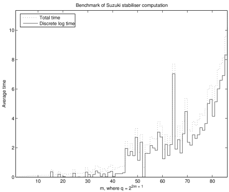
Figure 6.1. Benchmark of Suzuki stabiliser computation

In Figure 6.2 we show the benchmark of the algorithm in Theorem 3.17. For each field size, we made $100$ runs of the algorithms, using random generating sets of random conjugates of $\operatorname{Sz}(q)$.

The time complexity stated in the theorem suggests that the graph should be slightly worse than linear. Figure 6.2 clearly supports this. The minor oscillations can have at least two reasons. The algorithm is randomised, and the core of the algorithm is to find an element of order $q-1$ by random search. The proportion of such elements is $\phi(q-1)/(2(q-1))$ which oscillates slightly when $q$ increases.

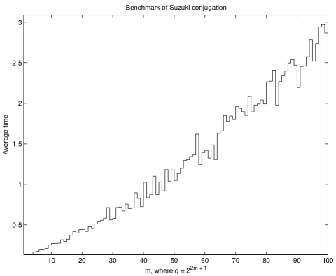
Figure 6.2. Benchmark of Suzuki conjugation

We do not include graphs of the tensor decomposition algorithms for the Suzuki groups. The reason is that at the present time, they can only be executed on a small number of inputs (certainly not more than $d\in\left\{16,64,256\right\}$ and $q\in\left\{8,32,128\right\}$) before running out of memory. Hence there is not much of a graph to display.

6.2. Small Ree groups

In the cases of the small Ree groups, the field size is always $q=3^{2m+1}$ for some $m>0$. Hence we display the time against $m$.

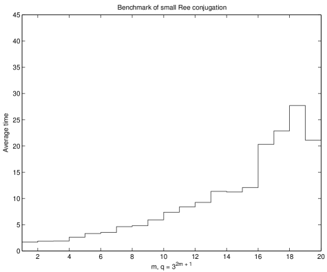
Figure 6.3. Benchmark of small Ree conjugation

In Figure 6.3 we show the benchmark of the algorithm in Theorem 3.47. For each field size, we made $100$ runs of the algorithms, using random generating sets of random conjugates of $\operatorname{Ree}(q)$. As can be seen from the proof of the Theorem, the algorithm involves many ingredients: discrete logarithms, $\operatorname{\mathtt{SLP}}$ evaluations, $\operatorname{SL}(2,q)$ recognition. To avoid making the graph unreadable, we avoid displaying the timings for these various steps, and only display the total time. The graph still has jumps, for reasons similar as with the Suzuki groups.

We do not include graphs of the tensor decomposition algorithms for the small Ree groups. The reason is that at the present time, they can only be executed on a small number of inputs (certainly not more than $d\in\left\{49,189,729\right\}$ and $q\in\left\{27,243\right\}$) before running out of memory. Hence there is not much of a graph to display.

6.3. Big Ree groups

In the cases of the Big Ree groups, the field size is always $q=2^{2m+1}$ for some $m>0$. Hence we display the time against $m$.

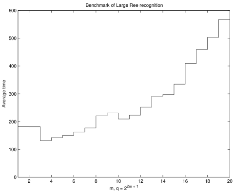
Figure 6.4. Benchmark of Large Ree conjugation

In Figure 6.4 we show the benchmark of the algorithm in Theorem 3.79. This involves all the results presented for the Big Ree groups.

For each field size, we made $100$ runs of the algorithms, using random generating sets of random conjugates of $\operatorname{{{}^{2}}F_{4}}(q)$. As can be seen from the proof of the Theorem, the algorithm involves many ingredients: discrete logarithms, $\operatorname{\mathtt{SLP}}$ evaluations, $\operatorname{Sz}(q)$ recognition, $\operatorname{SL}(2,q)$ recognition. To avoid making the graph unreadable, we avoid displaying the timings for these various steps, and only display the total time.

Bibliography

- [Asc84] M. Aschbacher, On the maximal subgroups of the finite classical groups, Invent. Math. 76 (1984), no. 3, 469–514. MR MR746539 (86a:20054)
- [Bab91] László Babai, Local expansion of vertex-transitive graphs and random generation in finite groups, STOC ’91: Proceedings of the twenty-third annual ACM symposium on Theory of computing (New York, NY, USA), ACM Press, 1991, pp. 164–174.
- [BB99] László Babai and Robert Beals, A polynomial-time theory of black box groups. I, Groups St. Andrews 1997 in Bath, I, London Math. Soc. Lecture Note Ser., vol. 260, Cambridge Univ. Press, Cambridge, 1999, pp. 30–64. MR MR1676609 (2000h:20089)
- [BB07] John Bray and Henrik Bäärnhielm, Standard generators for the Suzuki groups, preprint, 2007.
- [BK01] Peter A. Brooksbank and William M. Kantor, On constructive recognition of a black box , Groups and computation, III (Columbus, OH, 1999), Ohio State Univ. Math. Res. Inst. Publ., vol. 8, de Gruyter, Berlin, 2001, pp. 95–111. MR MR1829473 (2002m:20078)
- [BK06] by same author, Fast constructive recognition of black box orthogonal groups, J. Algebra 300 (2006), no. 1, 256–288. MR MR2228648
- [BKPS02] László Babai, William M. Kantor, Péter P. Pálfy, and Ákos Seress, Black-box recognition of finite simple groups of Lie type by statistics of element orders, J. Group Theory 5 (2002), no. 4, 383–401. MR MR1931364 (2003i:20022)
- [Bra00] John N. Bray, An improved method for generating the centralizer of an involution, Arch. Math. (Basel) 74 (2000), no. 4, 241–245. MR MR1742633 (2001c:20063)
- [Bra07] by same author, Presentations of the Suzuki groups, preprint, 2007.
- [Bro03a] Peter A. Brooksbank, Constructive recognition of classical groups in their natural representation, J. Symbolic Comput. 35 (2003), no. 2, 195–239. MR MR1958954 (2004c:20082)
- [Bro03b] by same author, Fast constructive recognition of black-box unitary groups, LMS J. Comput. Math. 6 (2003), 162–197 (electronic). MR MR2051584 (2005e:20075)
- [BS84] László Babai and Endre Szemerédi, On the complexity of matrix group problems, I, Proc. th IEEE Sympos. Foundations Comp. Sci., 1984, pp. 229–240.
- [CKSU05] Henry Cohn, Robert Kleinberg, Balazs Szegedy, and Christopher Umans, Group-theoretic algorithms for matrix multiplication, FOCS ’05: Proceedings of the 46th Annual IEEE Symposium on Foundations of Computer Science (Washington, DC, USA), IEEE Computer Society, 2005, pp. 379–388.
- [CLG97] Frank Celler and C. R. Leedham-Green, Calculating the order of an invertible matrix, Groups and computation, II (New Brunswick, NJ, 1995), DIMACS Ser. Discrete Math. Theoret. Comput. Sci., vol. 28, Amer. Math. Soc., Providence, RI, 1997, pp. 55–60. MR MR1444130 (98g:20001)
- [CLG01] Marston Conder and Charles R. Leedham-Green, Fast recognition of classical groups over large fields, Groups and computation, III (Columbus, OH, 1999), Ohio State Univ. Math. Res. Inst. Publ., vol. 8, de Gruyter, Berlin, 2001, pp. 113–121. MR MR1829474 (2002g:20001)
- [CLGM+95] Frank Celler, Charles R. Leedham-Green, Scott H. Murray, Alice C. Niemeyer, and E. A. O’Brien, Generating random elements of a finite group, Comm. Algebra 23 (1995), no. 13, 4931–4948. MR MR1356111 (96h:20115)
- [CLGO06] M. D. E. Conder, C. R. Leedham-Green, and E. A. O’Brien, Constructive recognition of , Trans. Amer. Math. Soc. 358 (2006), no. 3, 1203–1221 (electronic). MR MR2187651 (2006j:20017)
- [Cop84] Don Coppersmith, Fast evaluation of logarithms in fields of characteristic two, IEEE Trans. Inform. Theory 30 (1984), no. 4, 587–594. MR MR755785 (85h:65041)
- [CR06] Charles W. Curtis and Irving Reiner, Representation theory of finite groups and associative algebras, AMS Chelsea Publishing, Providence, RI, 2006, Reprint of the 1962 original. MR MR2215618 (2006m:16001)
- [CW90] Don Coppersmith and Shmuel Winograd, Matrix multiplication via arithmetic progressions, J. Symbolic Comput. 9 (1990), no. 3, 251–280. MR MR1056627 (91i:68058)
- [DS99] Huiwen Deng and Wujie Shi, The characterization of Ree groups by their element orders, J. Algebra 217 (1999), no. 1, 180–187. MR MR1700483 (2000i:20038)
- [Gie95] Mark Giesbrecht, Nearly optimal algorithms for canonical matrix forms, SIAM J. Comput. 24 (1995), no. 5, 948–969. MR MR1350753 (96f:65180)
- [GL01] Robert M. Guralnick and Frank Lübeck, On -singular elements in Chevalley groups in characteristic , Groups and computation, III (Columbus, OH, 1999), Ohio State Univ. Math. Res. Inst. Publ., vol. 8, de Gruyter, Berlin, 2001, pp. 169–182. MR MR1829478 (2002d:20074)
- [GLGO06] S. P. Glasby, C. R. Leedham-Green, and E. A. O’Brien, Writing projective representations over subfields, J. Algebra 295 (2006), no. 1, 51–61. MR MR2188850 (2006h:20002)
- [GM93] Daniel M. Gordon and Kevin S. McCurley, Massively parallel computation of discrete logarithms, CRYPTO ’92: Proceedings of the 12th Annual International Cryptology Conference on Advances in Cryptology (London, UK), Springer-Verlag, 1993, pp. 312–323.
- [HB82] Bertram Huppert and Norman Blackburn, Finite groups. III, Grundlehren der Mathematischen Wissenschaften [Fundamental Principles of Mathematical Sciences], vol. 243, Springer-Verlag, Berlin, 1982. MR MR662826 (84i:20001b)
- [HEO05] Derek F. Holt, Bettina Eick, and Eamonn A. O’Brien, Handbook of computational group theory, Discrete Mathematics and its Applications (Boca Raton), Chapman & Hall/CRC, Boca Raton, FL, 2005. MR MR2129747 (2006f:20001)
- [HLO+06] P. E. Holmes, S.A. Linton, E. A. O’Brien, A. J. E. Ryba, and R. A. Wilson, Constructive membership testing in black-box groups, preprint, 2006.
- [HR94] Derek F. Holt and Sarah Rees, Testing modules for irreducibility, J. Austral. Math. Soc. Ser. A 57 (1994), no. 1, 1–16. MR MR1279282 (95e:20023)
- [HRD05] Derek F. Holt and Colva M. Roney-Dougal, Constructing maximal subgroups of classical groups, LMS J. Comput. Math. 8 (2005), 46–79 (electronic). MR MR2123130 (2005k:20027)
- [HW79] G. H. Hardy and E. M. Wright, An introduction to the theory of numbers, fifth ed., The Clarendon Press Oxford University Press, New York, 1979. MR MR568909 (81i:10002)
- [IKS95] I. M. Isaacs, W. M. Kantor, and N. Spaltenstein, On the probability that a group element is -singular, J. Algebra 176 (1995), no. 1, 139–181. MR MR1345299 (96f:20035)
- [IL00] Gábor Ivanyos and Klaus Lux, Treating the exceptional cases of the MeatAxe, Experiment. Math. 9 (2000), no. 3, 373–381. MR MR1795309 (2001j:16067)
- [Kle88] Peter B. Kleidman, The maximal subgroups of the Chevalley groups with odd, the Ree groups , and their automorphism groups, J. Algebra 117 (1988), no. 1, 30–71. MR MR955589 (89j:20055)
- [KLM01] Gregor Kemper, Frank Lübeck, and Kay Magaard, Matrix generators for the Ree groups , Comm. Algebra 29 (2001), no. 1, 407–413. MR MR1842506 (2002e:20025)
- [LG01] Charles R. Leedham-Green, The computational matrix group project, Groups and computation, III (Columbus, OH, 1999), Ohio State Univ. Math. Res. Inst. Publ., vol. 8, de Gruyter, Berlin, 2001, pp. 229–247. MR MR1829483 (2002d:20084)
- [LGM02] C. R. Leedham-Green and Scott H. Murray, Variants of product replacement, Computational and statistical group theory (Las Vegas, NV/Hoboken, NJ, 2001), Contemp. Math., vol. 298, Amer. Math. Soc., Providence, RI, 2002, pp. 97–104. MR MR1929718 (2003h:20003)
- [LGO97a] C. R. Leedham-Green and E. A. O’Brien, Recognising tensor products of matrix groups, Internat. J. Algebra Comput. 7 (1997), no. 5, 541–559. MR MR1470352 (98h:20018)
- [LGO97b] by same author, Tensor products are projective geometries, J. Algebra 189 (1997), no. 2, 514–528. MR MR1438187 (98b:20073)
- [LL91] Y. N. Lakshman and Daniel Lazard, On the complexity of zero-dimensional algebraic systems, Effective methods in algebraic geometry (Castiglioncello, 1990), Progr. Math., vol. 94, Birkhäuser Boston, Boston, MA, 1991, pp. 217–225. MR MR1106424 (92d:13017)
- [LN85] V. M. Levchuk and Ya. N. Nuzhin, The structure of Ree groups, Algebra i Logika 24 (1985), no. 1, 26–41, 122. MR MR816569 (87h:20085)
- [LS74] Vicente Landazuri and Gary M. Seitz, On the minimal degrees of projective representations of the finite Chevalley groups, J. Algebra 32 (1974), 418–443. MR MR0360852 (50 #13299)
- [Lüb01] Frank Lübeck, Small degree representations of finite Chevalley groups in defining characteristic, LMS J. Comput. Math. 4 (2001), 135–169 (electronic). MR MR1901354 (2003e:20013)
- [Luk92] Eugene M. Luks, Computing in solvable matrix groups, IEEE Symposium on Foundations of Computer Science, 1992, pp. 111–120.
- [LW98] Klaus Lux and Markus Wiegelmann, Condensing tensor product modules, The atlas of finite groups: ten years on (Birmingham, 1995), London Math. Soc. Lecture Note Ser., vol. 249, Cambridge Univ. Press, Cambridge, 1998, pp. 174–190. MR MR1647421 (99i:20018)
- [Mal91] Gunter Malle, The maximal subgroups of , J. Algebra 139 (1991), no. 1, 52–69. MR MR1106340 (92d:20068)
- [MSC96] D. S. Mitrinović, J. Sándor, and B. Crstici, Handbook of number theory, Mathematics and its Applications, vol. 351, Kluwer Academic Publishers Group, Dordrecht, 1996. MR MR1374329 (97f:11001)
- [OL05] Eamonn A. OB́rien and Martin W. Liebeck, Finding the characteristic of a group of Lie type, J. London Math. Soc. (2005), to appear.
- [Ono62] Takashi Ono, An identification of Suzuki groups with groups of generalized Lie type., Ann. of Math. (2) 75 (1962), 251–259. MR MR0132780 (24 #A2616)
- [Ono63] by same author, Correction to “An identification of Suzuki groups with groups of generalized Lie type”, Ann. of Math. (2) 77 (1963), 413. MR MR0144967 (26 #2507)
- [Pak00] Igor Pak, The product replacement algorithm is polynomial, FOCS ’00: Proceedings of the 41st Annual Symposium on Foundations of Computer Science (Washington, DC, USA), IEEE Computer Society, 2000, pp. 476–485.
- [Pak01] by same author, What do we know about the product replacement algorithm?, Groups and computation, III (Columbus, OH, 1999), Ohio State Univ. Math. Res. Inst. Publ., vol. 8, de Gruyter, Berlin, 2001, pp. 301–347. MR MR1829489 (2002d:20107)
- [Par84] R. A. Parker, The computer calculation of modular characters (the meat-axe), Computational group theory (Durham, 1982), Academic Press, London, 1984, pp. 267–274. MR MR760660 (85k:20041)
- [R D05] R Development Core Team, R: A language and environment for statistical computing, R Foundation for Statistical Computing, Vienna, Austria, 2005, 3-900051-07-0.
- [Ree60] Rimhak Ree, A family of simple groups associated with the simple Lie algebra of type , Bull. Amer. Math. Soc. 66 (1960), 508–510. MR MR0125154 (23 #A2460a)
- [Ree61a] by same author, A family of simple groups associated with the simple Lie algebra of type , Bull. Amer. Math. Soc. 67 (1961), 115–116. MR MR0125155 (23 #A2460b)
- [Ree61b] by same author, A family of simple groups associated with the simple Lie algebra of type , Amer. J. Math. 83 (1961), 401–420. MR MR0132781 (24 #A2617)
- [Ree61c] by same author, A family of simple groups associated with the simple Lie algebra of type , Amer. J. Math. 83 (1961), 432–462. MR MR0138680 (25 #2123)
- [Rón90] Lajos Rónyai, Computing the structure of finite algebras, J. Symbolic Comput. 9 (1990), no. 3, 355–373. MR MR1056632 (91h:68093)
- [Ser03] Ákos Seress, Permutation group algorithms, Cambridge Tracts in Mathematics, vol. 152, Cambridge University Press, Cambridge, 2003. MR MR1970241 (2004c:20008)
- [Shi74] Ken-ichi Shinoda, The conjugacy classes of Chevalley groups of type over finite fields of characteristic , J. Fac. Sci. Univ. Tokyo Sect. I A Math. 21 (1974), 133–159. MR MR0349863 (50 #2356)
- [Shi75] by same author, The conjugacy classes of the finite Ree groups of type , J. Fac. Sci. Univ. Tokyo Sect. I A Math. 22 (1975), 1–15. MR MR0372064 (51 #8281)
- [Shp99] Igor E. Shparlinski, Finite fields: theory and computation, Mathematics and its Applications, vol. 477, Kluwer Academic Publishers, Dordrecht, 1999, The meeting point of number theory, computer science, coding theory and cryptography. MR MR1745660 (2001g:11188)
- [Sta06] Mark James Stather, Algorithms for computing with finite matrix groups, Ph.D. thesis, University of Warwick, August 2006.
- [Ste63] Robert Steinberg, Representations of algebraic groups, Nagoya Math. J. 22 (1963), 33–56. MR MR0155937 (27 #5870)
- [Ste77] by same author, On theorems of Lie-Kolchin, Borel, and Lang, Contributions to algebra (collection of papers dedicated to Ellis Kolchin), Academic Press, New York, 1977, pp. 349–354. MR MR0466336 (57 #6216)
- [Ste97] Allan Steel, A new algorithm for the computation of canonical forms of matrices over fields, J. Symbolic Comput. 24 (1997), no. 3-4, 409–432, Computational algebra and number theory (London, 1993). MR MR1484489 (98m:65070)
- [Str69] Volker Strassen, Gaussian elimination is not optimal, Numer. Math. 13 (1969), 354–356. MR MR0248973 (40 #2223)
- [Suz60] Michio Suzuki, A new type of simple groups of finite order, Proc. Nat. Acad. Sci. U.S.A. 46 (1960), 868–870. MR MR0120283 (22 #11038)
- [Suz62] by same author, On a class of doubly transitive groups, Ann. of Math. (2) 75 (1962), 105–145. MR MR0136646 (25 #112)
- [Suz64] by same author, On a class of doubly transitive groups. II, Ann. of Math. (2) 79 (1964), 514–589. MR MR0162840 (29 #144)
- [SZ93] Gary M. Seitz and Alexander E. Zalesskii, On the minimal degrees of projective representations of the finite Chevalley groups. II, J. Algebra 158 (1993), no. 1, 233–243. MR MR1223676 (94h:20017)
- [Tho01] Emmanuel Thomé, Computation of discrete logarithms in , Advances in cryptology—ASIACRYPT 2001 (Gold Coast), Lecture Notes in Comput. Sci., vol. 2248, Springer, Berlin, 2001, pp. 107–124. MR MR1934518 (2003h:94051)
- [vzGG03] Joachim von zur Gathen and Jürgen Gerhard, Modern computer algebra, second ed., Cambridge University Press, Cambridge, 2003. MR MR2001757 (2004g:68202)
- [War63] Harold N. Ward, On Ree’s series of simple groups, Bull. Amer. Math. Soc. 69 (1963), 113–114. MR MR0141707 (25 #5104)
- [War66] by same author, On Ree’s series of simple groups, Trans. Amer. Math. Soc. 121 (1966), 62–89. MR MR0197587 (33 #5752)
- [Wil05] R. A. Wilson, Finite simple groups, preprint, 2005.
- [Wil06] by same author, Elementary constructions of the Ree groups, preprint, 2006.
- [WP06] R. A. Wilson and C. W. Parker, Recognising simplicity of black-box groups, submitted (2006).