A route to high temperature superconductivity in composite systems

Abstract

Apparently, some form of local superconducting pairing persists to temperatures well above the maximum observed $T_{c}$ in underdoped cuprates, i.e. $T_{c}$ is suppressed due to the small phase stiffness. With this in mind, we consider the following question – Given a system with a high pairing scale $\Delta_{0}$ but with $T_{c}$ reduced by phase fluctuations, can one design a composite system in which $T_{c}$ approaches its mean-field value, $T_{c}\to T_{MF}\approx\Delta_{0}/2\,$? Here, we study a simple two component model in which a “metallic layer” with $\Delta_{0}=0$ is coupled by single-particle tunneling to a “pairing layer” with $\Delta_{0}>0$ but zero phase stiffness. We show that in the limit that the bandwidth of the metal is much larger than $\Delta_{0}$, $T_{c}$ of the composite system can reach the upper limit $T_{c}\approx\Delta_{0}/2$.

I Introduction

There are both theoreticalEmeryKivelson ; ourreview and experimentalourreview ; Uemura ; Corson ; Ong indications that underdoped cuprate superconductors can exhibit significant pairing correlations for a range of temperatures that extends above the highest measured superconducting $T_{c}$. Whereas in conventional metallic superconductors, $T_{c}\approx\Delta_{0}/2$ is determined by the pairing (zero $T$ gap) scale, in underdoped cuprates it is apparently determined by the collective onset of phase coherence, and hence by the superfluid stiffness, $\kappa\propto\rho_{s}$, where $\rho_{s}$ is the zero $T$ superfluid densityUemura .

The question we address here is: Given a material which has a “high” pairing scale, $\Delta_{0}$, but which fails to become a superconductor at high temperatures due to its low superfluid density, can we design an artificial composite of this material and a simple metal that realizes a high transition temperature, $T_{c}\sim\Delta_{0}/2\,$? Certainly superconductivity can be induced in the simple metal via the proximity effectmerchant , leading to an enhancement of the total superfluid density. Conversely, however, the pairing scale tends to be suppressed by the very same proximity effectmerchant ; valles . It is not clear, a priori, whether the composite will exhibit the best of both worlds, or the worst.

Two sets of experimental observations suggest a positive outcome. Firstly, in the last several years, Ong and collaboratorsOng have shown that phenomena related to fluctuation diamagnetism persist to moderately high temperatures in underdoped cuprates. This, added to the older evidence that there exists a spectroscopic pseudo-gap which extends to high temperatures, encourages us to interpret at least a portion of the observed “pseudo-gap regime” as a regime of pairing without global phase coherence. Secondly, recent experiments by Yuli et al. Millo on epitaxial films of La_2-xSr_xCuO₄ on a SrTiO substrate demonstrated that $T_{c}$ of underdoped films may be raised by depositing a thin upper-layer of strongly overdoped and hence metallic La_1.65Sr_0.35CuO₄ (see also Ref. [bozovic, ]).

Motivated by these findings, we study simple model systems composed of two components: a “pairing” component with a high pairing scale, $\Delta_{0}$, but zero $T_{c}$ due to zero superfluid stiffness, and a “metallic” component with no pairing but high stiffness. The microscopic origin of the pairing is not elucidated in this work, and we treat it as given. However, on physical grounds, we only consider situations in which $\Delta_{0}\ll E_{F}$, the Fermi energy of the metal. The two systems are coupled by a tunnelling matrix element $t_{\perp}$. Our principle result is the demonstration that, under the right conditions (i.e. the optimal magnitude of $t_{\perp}$), $T_{c}\approx\Delta_{0}/2$ can be achieved. It is our hope that these results can provide guidance for a new generation of searches, of the sort pioneered by Yuli et al.Millo , for higher temperature superconductivity in engineered composite materials. More generally, this work extends previous worksudip ; ekz ; physica ; arrigoni ; martin ; refael ; hongwei ; fradkin on “optimal inhomogeneity for superconductivity” to situations more amenable to direct experimental manipulation.

This paper is organized as follows. In Sec. II we describe the model and our strategy of solving it. The results for the cases in which the pairing layer consists of negative-$U$ sites and negative-$U$ wires are presented in Sections III and IV, respectively. The results are discussed in Sec. V.

II model and strategy

The “pairing component” is modelled by a two dimensional lattice of negative $U$ sites, which are either decoupled completely or coupled only in one direction (forming an array of parallel one-dimensional wires). In both cases, $T_{c}$ of the isolated pairing layer is zero due to zero phase stiffness. Nevertheless, the system has a finite pairing scale $\Delta_{0}$. Upon coupling this layer to a metallic layer modelled by non-interacting electrons, a finite $T_{c}$ obtains. The behavior of $T_{c}$ as a function of the strength of the coupling between the two systems is then studied.

The model Hamiltonian is

$$H=H_{c}+H_{f}+H_{cf}\text{,}$$ (1)

where $H_{c}$ is the Hamiltonian of the non-interacting (metallic) layer :

$$H_{c}=-t\sum_{\left\langle\mathbf{rr}^{\prime}\right\rangle\sigma}c_{\mathbf{r}\sigma}^{\dagger}c_{\mathbf{r}^{\prime}\sigma}^{\vphantom{\dagger}}+\mathrm{H.c.}-\mu\sum_{\mathbf{r}}n_{c,\mathbf{r}}\text{,}$$ (2)

where $\left\langle\mathbf{rr}^{\prime}\right\rangle$ denotes nearest neighbors. $H_{f}$ is the Hamiltonian of the “pairing” layer:

$$H_{f} = -(\mu-\varepsilon)\sum_{\mathbf{r}}n_{f,\mathbf{r}}$$ (3)

$$-U\sum_{\mathbf{r}}\left(n_{f,\mathbf{r}\uparrow}-\frac{1}{2}\right)\left(n_{f,\mathbf{r}\downarrow}-\frac{1}{2}\right)$$

$$-t^{\prime}\sum_{\mathbf{r\sigma}}f_{\mathbf{r}\sigma}^{\dagger}f_{\mathbf{r}+a\mathbf{\hat{x}},\sigma}^{\vphantom{\dagger}}+\mathrm{H.c.}$$

with $U>0$ (attractive) and $t^{\prime}=0$ for the “pairing sites” problem analyzed in Sec. III, and $t^{\prime}=t$ for the superconducting wires problem analyzed in Sec. IV. Finally, $H_{cf}$ is the the tunneling Hamiltonian between the two layers,

$$H_{cf}=-t_{\perp}\sum_{\mathbf{r}\sigma}c_{\mathbf{r}\sigma}^{\dagger}f_{\mathbf{r}\sigma}+\mathrm{H.c.}$$ (4)

Here $c_{\mathbf{r}\sigma}^{\dagger}$ and $f_{\mathbf{r}\sigma}^{\dagger}$ create electrons in the metallic and pairing layers, respectively, $n_{\mathbf{r}}=$ $n_{f,\mathbf{r}}+n_{c,\mathbf{r}}$ where $n_{f,\mathbf{r}}=\sum_{\sigma=\uparrow,\downarrow}$ $f_{\mathbf{r}\sigma}^{\dagger}$ $f_{\mathbf{r}\sigma}$, and similarly for $n_{c,\mathbf{r}}$. The on-site energy $\varepsilon$ for the $f$ sites is assumed to be close to the chemical potential, so that the $f$ band is partially filled. Throughout the analysis, we assume that the metallic bandwidth $W=8t$ is much larger than $t_{\perp}$, $U$. For simplicity, we consider the case of a two-dimensional square lattice, with a lattice constant $a=1$.

In order to solve (1), we first use mean-field theory to decouple the interaction term:

$$-Uf_{\mathbf{r\downarrow}}^{\dagger}f_{\mathbf{r\uparrow}}^{\dagger}f_{\mathbf{r\uparrow}}^{\vphantom{\dagger}}f_{\mathbf{r\downarrow}}^{\vphantom{\dagger}}\rightarrow-\Delta^{\ast}f_{\mathbf{r\uparrow}}^{\vphantom{\dagger}}f_{\mathbf{r\downarrow}}^{\vphantom{\dagger}}-\Delta f_{\mathbf{r\downarrow}}^{\dagger}f_{\mathbf{r\uparrow}}^{\dagger}+\delta\varepsilon n_{f,\mathbf{r}}\text{,}$$ (5)

and solve the self-consistent BCS equations at finite temperature:

$$\Delta=U\left\langle f_{\mathbf{r\uparrow}}f_{\mathbf{r\downarrow}}\right\rangle,$$ (6)

$$\delta\varepsilon=-\frac{U}{2}\langle n_{f,\mathbf{r}}\rangle,$$ (7)

$$n=\left\langle n_{\mathbf{r}}\right\rangle\text{,}$$ (8)

where $n$ is some fixed density. From these equations we find the mean-field transition temperature $T_{MF}$, at which $\Delta$ vanishes. However, the actual $T_{c}$ of the model is lower than $T_{MF}$ due to phase fluctuations, which are particularly important in situations where the phase stiffness is small, i.e. when $t_{\perp}$ is small. (Note that when $t_{\perp}=0$, $T_{MF}>0$, but $T_{c}=0$. This is true regardless of $t^{\prime}$.)

We make an estimate of the superconducting $T_{c}$ that includes both the usual physics of pairing that is captured by BCS mean-field theory and the dominant effects of phase fluctuations, as follows: To begin with, we compute the mean-field approximation to the phase stiffness $\rho_{s}\left(T\right)$, defined as

$$\rho_{s}\left(T\right)=\frac{1}{\Omega}\frac{\partial^{2}F}{\partial q_{x}^{2}}\text{,}$$ (9)

where $F/\Omega$ is the free energy per unit area and $q_{x}$ is a phase twist in the $x$ direction, which enters the kinetic energy term in the Hamiltonian as:

$$-t\sum_{\left\langle\mathbf{rr}^{\prime}\right\rangle\sigma}c_{\mathbf{r}\sigma}^{\dagger}c_{\mathbf{r}^{\prime}\sigma}^{\vphantom{\dagger}}\rightarrow-t\sum_{\left\langle\mathbf{rr}^{\prime}\right\rangle\sigma}e^{i\frac{\mathbf{q}}{2}\mathbf{\cdot}\left(\mathbf{r}^{\prime}-\mathbf{r}\right)}c_{\mathbf{r}\sigma}^{\dagger}c_{\mathbf{r}^{\prime}\sigma}^{\vphantom{\dagger}}$$ (10)

(Eq. (9) is slightly modified in cases where $t^{\prime}\neq 0$, since then the stiffness is anisotropic, and the relevant quantity is the geometric mean of the stiffness in the $x$ and $y$ directions. This will be discussed in Sec. IV.) Then, we estimate the temperature at which the two dimensional Kosterlitz-Thouless transition (phase ordering) occurs in terms of the universal jump of the stiffness at criticality:

$$\rho_{s}\left(T_{c}\right)=\frac{2}{\pi}T_{c}.$$ (11)

This is still an overestimate as it neglects the renormalization of $\rho_{s}\left(T_{c}\right)$ due to phase fluctuations below $T_{c}$. Upon solving Eqs. (6-8,11), we estimate $T_{c}$ as a function of the model parameters. Although $T_{c}$ estimated in this way is always less than $T_{MF}$, where $\rho_{s}\left(T\right)$ vanishes, if the phase stiffness is very large (as in a conventional weakly coupled BCS superconductor), then $T_{c}\approx T_{MF}$.

The method described above to determine $T_{c}$ was applied in Ref. [denteneer, ] for the negative $U$ Hubbard model, and the results were compared with the results of Quantum Monte Carlo (QMC) simulationsmoreo_scalapino ; scalettar . Qualitative trends of the Monte-Carlo results at generic fillings were well reproduced by this methodnote-half-filling . Moreover, although the Monte-Carlo $T_{c}$ was always smaller than the estimated $T_{c}$, the two typically differ by no more than 30% - 50%. Therefore, even though the method is not quantitatively reliable in the intermediate to strong coupling regime, we do expect it to predict correctly the qualitative trends of $T_{c}$ as a function of the model parameters. We intend to check the results using Monte-Carlo methods in the future.

III negative U sites

Let us focus on the case $t^{\prime}=0$ in Eq. (3), in which the negative-$U$ sites are coupled only by tunnelling through the metallic layer. We fix $t$, $U$, $\varepsilon$ and $n$, always assuming that $U$, $t_{\perp}\ll W$, where $W=8t$ is the bandwidth of the metallic layer, and calculate $T_{c}\left(t_{\perp}\right)$ [$\mu$ is determined by Eq. (8)]. $n$ is chosen so that the band of negative $U$ sites is partially filled (so that the self-consistent solution satisfies $\mu\approx\varepsilon+\delta\varepsilon$ and $\Delta\neq 0$ at $T=0$).

III.1 Analytical results

In the limit $t_{\perp}$, $T\ll U$, the dependence of $T_{c}$ on $t_{\perp}$ can be understood analytically from (4^th order) perturbation theory in $t_{\perp}$. In this limit, we may assume that $\Delta$ is approximately temperature independent and equal to its zero temperature value $\Delta_{0}\approx U/2$. At $T=0$, the perturbative expression is complicated due to Fermi surface singularities, but for temperatures in the important range $\Delta_{0}\gg T\gg t_{\perp}^{2}/\Delta_{0}$, the results simplify [see Appendix A, Eq. (30)]:

$$\rho_{s}\left(\frac{t_{\perp}^{2}}{U}\ll T\ll U\right)\sim\frac{t_{\perp}^{4}}{U^{2}T^{2}}\left\langle\mathbf{v}_{F}^{2}\right\rangle_{FS}N\left(0\right),$$ (12)

where $N\left(0\right)$ is the density of states of the metallic layer at the Fermi energy, and $\left\langle\mathbf{v}_{F}^{2}\right\rangle_{FS}$ is the square of its Fermi velocity averaged over the Fermi surface. Numerical factors of the order of unity have been dropped. Since parametrically $\left\langle\mathbf{v}_{F}^{2}\right\rangle_{FS}N\left(0\right)\sim t$, this gives $\rho_{s}\left(T\right)\sim\frac{t_{\perp}^{4}}{U^{2}T^{2}}t$. Using Eq. (11), we get the following estimate of $T_{c}$:

$$T_{c}\left(t_{\perp}\ll U\right)\sim t\left(\frac{t_{\perp}}{\sqrt{Ut}}\right)^{\frac{4}{3}}\text{.}$$ (13)

Eq. (13) gives that $T_{c}\gg$ $t_{\perp}^{2}/U$, consistent with the assumptions leading to Eq. (12). Eq. (13) must break down before $t_{\perp}\simeq t_{\perp,1}$ where

$$t_{\perp,1}\sim U\left(\frac{U}{t}\right)^{\frac{1}{4}}$$ (14)

since Eq. (13) gives $T_{c}\left(t_{\perp,1}\right)\sim U\sim\Delta_{0}$, and $T_{c}$ cannot exceed $\Delta_{0}$.

As $t_{\perp}$ is increased beyond $t_{\perp,1}$, the superfluid density is large enough and ceases to limit $T_{c}$ significantly. However, the pairing is also reduced. $T_{MF}$, the temperature at which $\Delta\left(T_{MF}\right)=0$, can be calculated perturbatively in $t_{\perp}$ [Eq. (38) of Appendix A]:

$$T_{MF}=\frac{U}{4}\left[1-\frac{At_{\perp}^{2}}{Ut}+O\left(t_{\perp}^{4}\right)\right],$$ (15)

where, to be explicit, we have taken the negative $U$ sites to be half filled for $t_{\perp}=0$. $A$ is a dimensionless number of order unity. Therefore $T_{MF}$ is not suppressed significantly from its $t_{\perp}=0$ limit until $t_{\perp}$ becomes of the order of

$$t_{\perp,2}\sim\sqrt{Ut}.$$ (16)

Interestingly, we see that in the limit $U\ll t$, the ratio $\frac{t_{\perp,2}}{t_{\perp,1}}=\left(\frac{t}{U}\right)^{\frac{3}{4}}$ becomes large. Therefore, there is a parametrically wide region where there is plenty of superfluid stiffness, but the pairing is still not suppressed significantly. It is at least plausible to expect that in the region $t_{\perp,1}\lesssim t_{\perp}\lesssim t_{\perp,2}$, $T_{c}$ of the order of $T_{MF}\left(t_{\perp}=0\right)\approx{\Delta_{0}}/{2}$ is obtained.

III.2 Numerical results

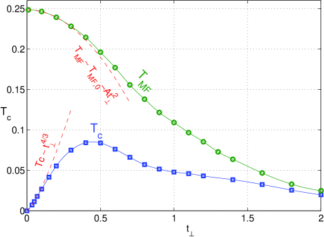
Figure 1: (Color online.) $T_{c}$ ($\square$) and $T_{MF}$ ($\circ$) obtained from solving Eqs. (6-8,9) numerically for $n=1.5$, $t=1$, $U=1$, as a function of $t_{\perp}$. The dashed curves are fits to the data according to Eqs. (13,15). $A=0.235$ was used in the fit.

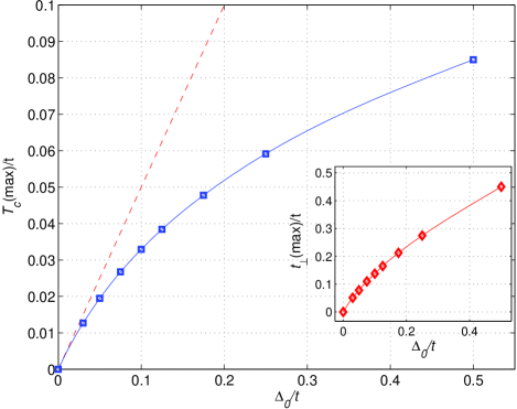
Figure 2: (Color online.) $T_{c}$(max) (maximized over $t_{\perp}$) for different values of $U$ and fixed $t=1$, $n=1.5$. $T_{c}$(max) is shown as a function of $\Delta_{0}\approx U/2$, which is the $T=0$, $t_{\perp}=0$ gap for the same $U$. The dashed line is the mean field transition temperature for $t_{\perp}=0$, $T_{MF,0}\approx\Delta_{0}/2$. inset: $t_{\perp}$(max) in which $T_{c}$(max) is obtained, as a function of $\Delta_{0}$.

Fig. 1 shows $T_{c}$ and $T_{MF}$ obtained from solving Eqs. (6-8,9) numerically for $n=1.5$, $t=1$, $\varepsilon=-1$ and $U=1$, as a function of $t_{\perp}$. At low $t_{\perp}$, $T_{MF}\approx U/4$, while $T_{c}$ is strongly suppressed due to the low superfluid stiffness. For low enough $t_{\perp}$, $T_{c}\sim t_{\perp}^{4/3}$ in agreement with Eq. (13). $T_{c}$ reaches a maximum at $t_{\perp}\approx 0.45$, and then starts to drop due to the suppression of $T_{MF}$. At high enough $t_{\perp}$, $T_{c}$ essentially coincides with $T_{MF}$. The maximum $T_{c}$, which is obtained in the crossover regime between pairing-dominated and stiffness-dominated regimes, is $T_{c}\approx 0.085$, which is about $35\%$ of the maximum $T_{MF}$.

In Fig. 2 we show $T_{c}\left(\max\right)$, which is the maximum of $T_{c}\left(t_{\perp}\right)$, as a function of $\Delta_{0}\approx U/2$, which is the $T=0$, $t_{\perp}=0$ gap. We fix $t=1$ and $n=1.5$ throughout the calculation. In the low $\Delta_{0}/t$ limit, $T_{c}\left(\max\right)$ reaches the maximum conceivable value which takes full advantage of the pairing scale, $T_{c}\left(\max\right)/\Delta_{0}\to A_{0}\approx 1/2$ as $\Delta_{0}/t\to 0$. (The dashed line in Fig. 2 is $T_{c}\left(\max\right)=\Delta_{0}/2$).

The optimal $t_{\perp}$ for superconductivity, $t_{\perp}$(max) is shown in the inset of Fig. 2 as a function of $\Delta_{0}$. For small $\Delta_{0}/t$, we find that $t_{\perp}$(max)$\approx\Delta_{0}$. As $\Delta_{0}$ is lowered, the maximum becomes broader and broader relative to $\Delta_{0}$, in agreement with what we expect from Eq. (14,16): $T_{c}\approx\Delta_{0}/2$ for $t_{\perp,1}\lesssim t_{\perp}\lesssim t_{\perp,2}$, and this range becomes parametrically wide at low $\Delta_{0}$.

IV superconducting wires

IV.1 Analytical results

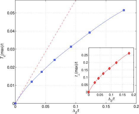
Figure 3: (Color online.) Same as Fig 2 for the case of superconducting wires [$t^{\prime}=t$ in Eq. (3)]. $T_{c}$(max)$/t$ (maximized over $t_{\perp}$) is shown as a function of $\Delta_{0}/t$. The dashed line shows the mean-field transition temperature at $t_{\perp}=0$, $T_{MF,0}/t\approx 2\Delta_{0}$/(3.5t). inset: $t_{\perp}$(max)$/t$ as a function of $\Delta_{0}/t$.

We now consider the case in which the “pairing layer” is an array of one dimensional wires in the $x$ direction. Assuming that $t^{\prime}\sim t>U$, the zero temperature gap is given by the BCS equation: $\Delta_{0}\sim t^{\prime}\exp[-1/\tilde{N}(0)U]$ where $\tilde{N}(0)\sim(2\pi t^{\prime})^{-1}$ is the density of states of a single wire. The phase stiffness along the $x$ direction is finite even for $t_{\perp}\rightarrow 0$,comment-wires1 while the stiffness in the $y$ direction vanishes at this limit. Since the phase stiffness is anisotropic, $\rho_{s}^{x}\neq\rho_{s}^{y}$, the macroscopic phase stiffness, which appear in Eq. (11), is an appropriate average of its values in the two directions. Analogously to the case of the anisotropic two dimensional $XY$ model, the geometric average of $\rho_{s}^{x}$, $\rho_{s}^{y}$ should be useddimcross :

$$\rho_{s}=\sqrt{\rho_{s}^{x}\rho_{s}^{y}}\text{.}$$ (17)

We have found that $T_{c}$ of the composite system is highest when the Fermi surfaces of the two layers intersect in the $t_{\perp}\to 0$, $U\to 0$ limit comment-wires2 . We therefore assume that this is the case in what follows.

Following a similar line of reasoning as in Sec. III, the scaling of $\rho_{s}$ in the limit $\frac{t_{\perp}^{2}}{\Delta_{0}}\ll T\ll\Delta_{0}$ is [Eq. (32) in Appendix A]:

$$\rho_{s}\left(\frac{t_{\perp}^{2}}{\Delta_{0}}\ll T\ll\Delta_{0}\right)\sim\sqrt{\frac{t}{\Delta_{0}}}\frac{t_{\perp}^{2}}{T}\text{,}$$ (18)

which by Eq. (11) gives

$$T_{c}\left(t_{\perp}\ll\Delta_{0}\right)\sim\left(\frac{t}{\Delta_{0}}\right)^{\frac{1}{4}}t_{\perp}\text{.}$$ (19)

And, since $T_{c}$ cannot exceed $\sim\Delta_{0}$, Eq. (19) can only hold for

$$t_{\perp}\lesssim t_{\perp,1}=\left(\frac{\Delta_{0}}{t}\right)^{\frac{1}{4}}\Delta_{0}\text{.}$$ (20)

The small $t_{\perp}$ behavior of $T_{MF}$ is [Eq. (41)]

$$T_{MF}\approx T_{MF,0}\left[1-\frac{\tilde{A}t_{\perp}^{2}}{tT_{MF,0}}+O\left(t_{\perp}^{4}\right)\right]\text{,}$$ (21)

where $T_{MF,0}=T_{MF}\left(t_{\perp}=0\right)\approx{\Delta_{0}}/{2}$ and $\tilde{A}$ is a dimensionless constant of order unity. Therefore, the suppression of $T_{MF}$ due to the coupling of the superconducting wires to the metallic layer becomes significant when

$$t_{\perp}\gtrsim t_{\perp,2}=\sqrt{\Delta_{0}t}\text{.}$$ (22)

Thus, as in the case of isolated negative-$U$ sites, there is a region between $t_{\perp,1}$ and $t_{\perp,2}$ where there is plenty of phase stiffness and the pairing is not suppressed significantly. Moreover, since ${t_{\perp,2}}/{t_{\perp,1}}\sim\left({t}/{\Delta_{0}}\right)^{\frac{3}{4}}$, this region becomes parametrically wide when $\Delta_{0}\ll t$. In that limit, we expect that $T_{c}$ can be asymptotically close to $T_{MF,0}$.

IV.2 Numerical results

Fig. 3 shows $T_{c}$(max) (maximized over $t_{\perp}$) as a function of $\Delta_{0}$ for the case of 1D wires. The following parameters were used: $t=t^{\prime}=1$, $\varepsilon=-1$ and $n=1.5$. $U$ was varied between $1.1$ and $1.65$. Also shown in the same figure is $T_{MF,0}$, the mean-field transition temperature of the wires for $t_{\perp}=0$. We found that in the range of $U$ we considered, $T_{MF,0}$ is very well approximated by the BCS formula $T_{MF,0}=2\Delta_{0}/3.5=a\exp(-b/U)$, with $a=4.415$ and $b=6.215$, i.e. $\Delta_{0}$ changes by an order of magnitude from $\Delta_{0}\approx 3\times 10^{-2}$ to $1.8\times 10^{-1}$. As in the case of the negative $U$ sites, in the limit $\Delta_{0}/W\to 0$, $T_{c}$(max) approaches $T_{MF,0}$.

The inset of Fig. 3 shows the optimal value of $t_{\perp}$ as a function of $\Delta_{0}$. For small $\Delta_{0}$, we see that $t_{\perp}$(max)$\approx 2\Delta_{0}$.

V discussion

The pairing scale $\Delta_{0}$ defines a physical limit on the maximum achievable superconducting $T_{c}$ in a given system. However, typically as the phase stiffness is increased, the pairing scale tends to be suppressed, and eventually this suppresses the actual $T_{c}$. Therefore, the maximum $T_{c}$ is typically reduced relative to $\Delta_{0}$, often by a large factor. For example, in the two-dimensional negative-$U$ Hubbard model with fixed $U$, the maximum possible $\Delta_{0}$ is about $U/2$, which is achieved for $t=0$ and close to half filling. However, the maximum $T_{c}$ (estimated by the method of combining the mean-field solution with classical phase fluctuations, as described in Sec. II) is only $0.085U$ (obtained for $t\approx 0.4U$).

In the present work, we have been motivated by the following question: Suppose that there exists a material with a large pairing scale, $\Delta_{0}$, but a low (or vanishing) $T_{c}$ due to phase fluctuations; is there a way to make a composite of this material and a good metal which will realize a superconducting state with a transition temperature, $T_{c}\to T_{MF,0}\approx\Delta_{0}/2\,$? In the two model systems we studied, we found that by weakly coupling the two materials with $t_{\perp}\sim\Delta_{0}$, and in the limit that the bandwidth of the metal is large, $W/\Delta_{0}\rightarrow\infty$, this optimal $T_{c}$ can be achieved.

This result was demonstrated using a physically motivated approximate solution of the model. Fortunately, the negative $U$ Hubbard model is amenable to solution on moderately large systems by Quantum Monte Carlo Methods, as it can be made free of fermion sign problemsdossantos . We therefore intend to test the validity of our results in this way in the near future.

Finally, we discuss the reasons to believe that our conclusions do not depend sensitively on the specifics of the models. The coupling of a paired material to a good metal produces two qualitatively different effects: an increased superfluid stiffness, $\delta\rho_{s}$, and a reduction of the mean field transition temperature by an amount $\delta T_{MF}$. It is clear that in the limit of strong coupling between the two systems, $t_{\perp}\sim W$ where $W$ is the metallic bandwidth, the latter effect always dominates, and hence coupling to the metal leads to a quenching of superconductivity.

Let us therefore consider $t_{\perp}\sim\Delta_{0}\ll W$, where a perturbative expression for $\delta T_{MF}$ will generally give

$$\delta T_{MF}=-AW^{-a}\Delta_{0}^{a-1}t_{\perp}^{2}\sim-W^{-a}\Delta_{0}^{a+1}.$$ (23)

where $A>0$ is a dimensionless constant, $a$ is an exponent which could differ from case to case, and in the final expression we have taken $t_{\perp}\sim\Delta_{0}$. Similarly, close to the putative superconducting transition temperature $T\approx\Delta_{0}/2$, we expect

$$\delta\rho_{s}=BW^{b}\Delta_{0}^{-1-b}|\Delta(T)|^{2},$$ (24)

where $B$ is another constant, and $|\Delta(T)|\ll\Delta_{0}$ is the temperature dependent mean field gap in the pairing layer. So long as $a>0$ and $b>0$, these relations imply that in the limit that $W\to\infty$, the induced phase stiffness at any $T<T_{MF,0}$ grows without bound with no significant loss of pairing. Hence phase fluctuations are suppressed, leading to $T_{c}\to T_{MF,0}$.

Generally, one expects that $\delta\rho_{s}$ increases as $W$ is increased (i.e. $b>0$), while $|\delta T_{MF}|$ decreases ($a>0$), since, in the metal, the Fermi velocity is a linearly increasing function and the Fermi energy density of states is a linearly decreasing function of $W$. Indeed, in the case of negative $U$ sites, $a=b=1$, comment-exponents a result which, we believe, is true in a wide range of circumstances.

As corroborating evidence, we note that the expected non-monotonic dependence of $T_{c}$ on coupling between a metal and a phase fluctuating superconductor has been observed in a somewhat analogous experimental systemmerchant consisting of Pb grains covered with a film of Ag. As a function of increasing Ag coverage, the first effect is to suppress phase fluctuations and to increase the superconducting transition temperature up to nearly the bulk $T_{c}$ of Pb. comment-merchant However, adding more Ag to the system eventually causes a degradation of the pairing scale and a total quenching of superconductivity.

As a concluding remark, we comment on the effect of the pairing symmetry on our results. So far we have considered cases where the superconducting order parameter has $s$-wave symmetry. In the case of $d$-wave symmetry, the induced order parameter in the metal has nodes. This will reduce the superfluid density at low temperature relative to the $s$-wave case, due to the excitation of nodal quasi-particles. However, at $T\approx\Delta_{0}/2$, the behavior of $\rho_{s}$ is not expected to be qualitatively different from the $s$-wave case. Therefore we expect our main results, $T_{c}$(max)$\approx\Delta_{0}/2$, to hold in the $d$-wave case as well. We intend to test this claim explicitly in the future.

Appendix A The low $t_{\perp}$ limit

A.1 Superfluid density

We will now derive Eqs. (12,18) for the superfluid density in the limit $\frac{t_{\perp}^{2}}{\Delta_{0}}\ll T\ll\Delta_{0}$, where $\Delta_{0}$ is the zero temperature gap in the “pairing layer”. In this limit, we assume that $\Delta\left(T\right)=\Delta_{0}$ is independent of temperature. We proceed by integrating out the (gapped) negative-$U$ layer degrees of freedom, obtaining an effective action for the metallic layer. Focusing on the low energy modes of the metallic layer, the $\omega$ dependence of the effective action can be neglected, obtaining a low-energy effective Hamiltonian of the form

$$H_{\text{eff}}=\sum_{\mathbf{k}\sigma}\xi_{\mathbf{k}+\frac{\mathbf{q}}{2}}c_{\mathbf{k}\sigma}^{\dagger}c_{\mathbf{k}\sigma}^{\vphantom{\dagger}}+\tilde{\Delta}\sum_{\mathbf{k}}c_{\mathbf{k}\uparrow}^{\dagger}c_{\mathbf{-k}\downarrow}^{\dagger}+\mathrm{H.c.}\text{,}$$ (25)

where $\xi_{\mathbf{k}}=-2t\left(\cos k_{x}+\cos k_{y}\right)-\mu$, $\mathbf{q}/2$ is a vector potential introduced in order to calculate the phase stiffness, and

$$\tilde{\Delta}\sim\frac{t_{\perp}^{2}}{\Delta_{0}}$$ (26)

is the proximity induced pairing field in the metallic layer. Note that in the $T\ll\Delta_{0}$ limit, $\tilde{\Delta}$ is approximately temperature independent, even for temperatures larger than $\tilde{\Delta}$. The phase stiffness at temperature $T$ is calculated from (25) in the standard way by computing the free energy $F\left(\mathbf{q}\right)=-T\ln Z\left(\mathbf{q}\right)$ where $Z\left(\mathbf{q}\right)=$Tr$\left[\exp\left(-\beta H_{\text{eff}}\right)\right]$, and differentiating twice the free energy per unit area with respect to $q_{x}$. This giveswhite_zhang_scalapino

$$\rho_{s} = \frac{1}{2\Omega}\sum_{\mathbf{k}}\left[u_{\mathbf{k}}^{2}f\left(E_{\mathbf{k}}\right)+v_{\mathbf{k}}^{2}\left(1-f\left(E_{\mathbf{k}}\right)\right)\right]\frac{\partial^{2}\xi_{\mathbf{k}}}{\partial k_{x}^{2}}$$ (27)

$$-\frac{1}{2\Omega}\sum_{\mathbf{k}}\left(\frac{\partial\xi_{\mathbf{k}}}{\partial k_{x}}\right)^{2}\beta f\left(E_{\mathbf{k}}\right)\left[1-f\left(E_{\mathbf{k}}\right)\right]\text{,}$$

where $E_{\mathbf{k}}=\sqrt{\tilde{\Delta}^{2}+\xi_{\mathbf{k}}^{2}}$, $u_{\mathbf{k}}=\sqrt{\frac{1}{2}\left(1+\frac{\xi_{\mathbf{k}}}{E_{\mathbf{k}}}\right)}$, $v_{\mathbf{k}}=\sqrt{\frac{1}{2}\left(1-\frac{\xi_{\mathbf{k}}}{E_{\mathbf{k}}}\right)}$ and $f\left(\varepsilon\right)$ is the Fermi function. Integrating the first line of Eq. (27) by parts and replacing $\int\frac{d^{2}k}{\left(2\pi\right)^{2}}\rightarrow\int d\xi N\left(\xi\right)$, where $N\left(\xi\right)$ is the density of states of the metallic layer, we get

$$\rho_{s} = \frac{1}{2}\int_{-W/2-\mu}^{W/2-\mu}d\xi N\left(\xi\right)\frac{\tilde{\Delta}^{2}}{E^{2}}{\Bigg{\{}}\frac{1}{2E}\tanh\left(\frac{\beta E}{2}\right)$$ (28)

$$-\beta f\left(E\right)\left[1-f\left(E\right)\right]{\Bigg{\}}}\left\langle\mathrm{v}_{x}^{2}\right\rangle\left(\xi\right)\text{.}$$

Here $E\left(\xi\right)=\sqrt{\xi^{2}+\tilde{\Delta}^{2}}$ and the averaged square velocity at energy $\xi$ of the metallic layer is $\left\langle\mathrm{v}_{x}^{2}\right\rangle\left(\xi\right)=\frac{1}{N\left(\xi\right)}\int\frac{d^{2}k}{\left(2\pi\right)^{2}}\delta\left(\xi_{\mathbf{k}}-\xi\right)\left(\frac{\partial\xi_{\mathbf{k}}}{\partial k_{x}}\right)^{2}$. Assuming $|\pm W/2-\mu|\gg T$ implies that the integral in Eq. (28) is dominated by energies close to the chemical potential. Hence, we may estimate it by replacing $N\left(\xi\right)$ and $\left\langle\mathrm{v}_{x}^{2}\right\rangle\left(\xi\right)$ by their values at the chemical potential (we assume that $\mu$ is not too close to zero in order to avoid the logarithmic divergence of $N(\xi)$ at the middle of the band). Changing variables to $\eta=\beta\sqrt{\xi^{2}+\tilde{\Delta}^{2}}$, we obtain

$$\rho_{s}\simeq\frac{\tilde{\Delta}^{2}}{T^{2}}N\left(0\right)\left\langle\mathrm{v}_{x}^{2}\right\rangle\left(0\right)\int_{\beta\tilde{\Delta}}^{\beta W}d\eta\frac{F\left(\eta\right)}{\eta\sqrt{\eta^{2}-\left(\beta\tilde{\Delta}\right)^{2}}}\text{,}$$ (29)

where $F\left(\eta\right)=\frac{1}{2\eta}\tanh\left(\frac{\eta}{2}\right)-\frac{e^{\eta}}{\left(1+e^{\eta}\right)^{2}}$. at low $\eta$, $F\left(\eta\right)=O\left(\eta^{2}\right)$, so the integral converges in the limit $\beta\tilde{\Delta}\rightarrow 0$. At high $\eta$, $F\left(\eta\right)\sim\frac{1}{\eta}$, so we may also take the $\beta W\rightarrow\infty$ limit. Therefore, we obtain to leading order in $\beta\tilde{\Delta}$ and $\frac{1}{\beta W}$

$$\rho_{s}\text{(neg. U sites)} \simeq \alpha\frac{\tilde{\Delta}^{2}}{T^{2}}N\left(0\right)\left\langle\mathrm{v}_{x}^{2}\right\rangle\left(0\right)$$ (30)

$$\sim \frac{t_{\perp}^{4}}{\Delta_{0}^{2}T^{2}}N\left(0\right)\left\langle\mathrm{v}_{x}^{2}\right\rangle\left(0\right),$$

where $\alpha=\int_{0}^{\infty}d\eta F\left(\eta\right)/\eta^{2}=7\zeta(3)/8\pi^{2}$, and we have used Eq. (26). This is Eq. (12). We have verified Eq. (30) by calculating $\rho_{s}$ using finite temperature perturbation theory to order $t_{\perp}^{4}$, by integrating out the fermions to obtain an effective action for the superconducting phase, and by evaluating Eq. (9) numerically in the low $t_{\perp}$ limit.

In the case of superconducting wires, the “pairing layer” has a finite stiffness of order $\rho_{s}^{x}\sim t^{\prime}$ in the $x$ direction (parallel to the wires) even in the $t_{\perp}\rightarrow 0$ limit. In the transverse direction, however, Eq. (30) applies for $\rho_{s}^{y}$, with the exception that now the proximity induced gap depends on $\mathbf{k}$. The induced gap is significant in a sliver in $\mathbf{k}$ space of width $\delta k_{x}\sim\frac{\Delta_{0}}{v_{F}^{\prime}}$ around the Fermi surface of the wires (where $v_{F}^{\prime}$ are the Fermi velocities of the wires), reaching a maximum of order $\frac{t_{\perp}^{2}}{\Delta_{0}}$, and negligible elsewhere (since only the region of Fermi surface of the wires has considerable particle-hole mixing). Taking $N(0)\left\langle\mathrm{v}_{y}^{2}\right\rangle\sim t$ and $v_{F}^{\prime}\sim t^{\prime}\sim t$, we therefore estimate $\rho_{s}^{y}$ in this case as

$$\rho_{s}^{y}\sim\frac{t_{\perp}^{4}t}{\Delta_{0}^{2}T^{2}}\left(\frac{\Delta_{0}}{t^{\prime}}\right)=\frac{t_{\perp}^{4}}{\Delta_{0}T^{2}}.$$ (31)

The geometric average of $\rho_{s}^{x}$ and $\rho_{s}^{y}$ (which determines $T_{c}$) scales as

$$\rho_{s}\left(\text{s.c. wires}\right)=\sqrt{\rho_{s}^{x}\rho_{s}^{y}}\sim\sqrt{\frac{t}{\Delta_{0}}}\frac{t_{\perp}^{2}}{T},$$ (32)

which is Eq. (18).

A.2 $T_{MF}$ in the low $t_{\perp}$ limit

$T_{MF}$ is obtained by the equation

$$U\chi_{SC}\left(T_{MF}\right)=1\text{,}$$ (33)

where $\chi_{SC}\left(T\right)$ is the superconducting susceptibility of the pairing layer with $\Delta=0$. Using finite temperature perturbation theory, $\chi_{SC}\left(T_{MF}\right)$ can be expanded in powers of $t_{\perp}$. Since we are dealing with a non-interacting theory, all the diagrams are straight lines with $t_{\perp}$ vertices along them. The leading order correction to $\chi_{SC}\left(T\right)$ is

$$\delta\chi_{SC}=\frac{2t_{\perp}^{2}a^{2}}{\beta\Omega}\sum_{i\omega_{n}\mathbf{k}}\frac{1}{i\omega_{n}+\varepsilon_{\mathbf{k}}}\frac{1}{\left(-i\omega_{n}+\varepsilon_{\mathbf{k}}\right)^{2}}\frac{1}{-i\omega_{n}+\xi_{\mathbf{k}}},$$ (34)

where the dispersions in the pairing and metallic layers are given by $\varepsilon_{\mathbf{k}}=-2t^{\prime}\cos k_{x}-(\mu-\varepsilon-\delta\varepsilon)$, and $\xi_{\mathbf{k}}=-2t\left(\cos k_{x}+\cos k_{y}\right)-\mu$, respectively. Here, $a^{2}$ is the unit cell area and $\omega_{n}=\frac{\left(2n+1\right)\pi}{\beta}$ are Matsubara frequencies. Performing the Matsubara summation, we obtain

$$\delta\chi_{SC}=\frac{2t_{\perp}^{2}a^{2}}{\Omega}\sum_{\mathbf{k}}\left[\frac{\left[\varepsilon_{\mathbf{k}}-\xi_{\mathbf{k}}\tanh\left(\beta\varepsilon_{\mathbf{k}}/2\right)\right]}{4\varepsilon_{\mathbf{k}}^{2}\left(\varepsilon_{\mathbf{k}}^{2}-\xi_{\mathbf{k}}^{2}\right)}+\frac{2f\left(\varepsilon_{\mathbf{k}}\right)\left[1-\beta f\left(-\varepsilon_{\mathbf{k}}\right)\left(-\varepsilon_{\mathbf{k}}+\xi_{\mathbf{k}}\right)\right]}{4\varepsilon_{\mathbf{k}}\left(-\varepsilon_{\mathbf{k}}+\xi_{\mathbf{k}}\right)^{2}}-\frac{f\left(\xi_{\mathbf{k}}\right)}{\left(\xi_{\mathbf{k}}+\varepsilon_{\mathbf{k}}\right)\left(-\xi_{\mathbf{k}}+\varepsilon_{\mathbf{k}}\right)^{2}}\right].$$ (35)

In the case of disconnected negative-$U$ sites, we take the limit $\varepsilon_{\mathbf{k}}\rightarrow 0$ in Eq. (35) (assuming that the negative-$U$ sites are close to half-filling). The limit gives

$$\delta\chi_{SC}\left(\text{neg. }U\text{ sites}\right) = -\frac{2t_{\perp}^{2}a^{2}}{\Omega}\sum_{\mathbf{k}}\frac{\beta\xi_{\mathbf{k}}-2\tanh\left(\frac{\beta\xi_{\mathbf{k}}}{2}\right)}{4\xi_{\mathbf{k}}^{3}}$$ (36)

$$\approx -\tilde{\alpha}\frac{t_{\perp}^{2}N\left(0\right)a^{2}}{T^{2}},$$

where $\tilde{\alpha}=\int_{0}^{\infty}dxx^{-3}\left[x-2\tanh\left(x/2\right)\right]=7\zeta(3)/2\pi^{2}$. We have replaced $N\left(\xi\right)\$by $N\left(0\right)$, which is a reasonable approximation since the integral is dominated by the low energy regime. Adding $\delta\chi_{SC}$ to the zeroth-order susceptibility $\chi_{SC}^{0}\approx\frac{1}{4T}$ of disconnected sites, we get from Eq. (33)

$$\frac{U}{4T_{MF}}\left[1-\frac{4\tilde{\alpha}N(0)a^{2}t_{\perp}^{2}}{T_{MF}}+O\left(t_{\perp}^{4}\right)\right]=1\text{.}$$ (37)

Solving for $T_{MF}$ to leading order in $t_{\perp}^{2}$, we get

$$T_{MF}\text{(neg. }U\text{ sites)}\approx\frac{U}{4}\left[1-\frac{At_{\perp}^{2}}{tU}+O\left(t_{\perp}^{4}\right)\right],$$ (38)

where $A=16\tilde{\alpha}tN(0)a^{2}\approx 2\tilde{\alpha}$, where $N(a)a^{2}\approx W^{-1}=(8t)^{-1}$ was used. This is Eq. (15).

In the case of superconducting wires, we can still estimate the parametric form of the most divergent part of $\delta\chi_{SC}$ at low temperatures. The strongest singularity of the integral in (35) comes from the vicinity of the crossing of the two Fermi surfaces (i.e. $\xi_{\mathbf{k}}=0$, $\varepsilon_{\mathbf{k}}=0$). This singularity is cut off by the temperature. As a rough estimation of the integral, we evaluate the integrand in the limit $\beta\left|\varepsilon_{\mathbf{k}}\right|$, $\beta\left|\xi_{\mathbf{k}}\right|\gg 1$, so that $\tanh\left(\frac{\beta\varepsilon_{\mathbf{k}}}{2}\right)\rightarrow$ sign$\left(\varepsilon_{\mathbf{k}}\right)$, $f\left(\varepsilon_{\mathbf{k}}\right)\rightarrow\Theta\left(-\varepsilon_{\mathbf{k}}\right)$ where $\Theta$ is a Heaviside step function, etc., and extend the integration only to within $T$ of the line $\varepsilon_{\mathbf{k}}=0$. Further, we change variables from $\mathbf{k}$ to $\left(\varepsilon_{\mathbf{k}},\xi_{\mathbf{k}}\right)$, with Jacobian $J\left(\varepsilon,\xi\right)=\frac{1}{\left|\nabla_{\mathbf{k}}\varepsilon\times\nabla_{\mathbf{k}}\xi\right|}$ which we replace by its value at $\left(\varepsilon=0,\xi=0\right)$. Adding the contributions in the four quadrants around the point $\left(\varepsilon=0,\xi=0\right)$ (both $\varepsilon$ and $\xi$ can be positive or negative), we get:

$$\delta\chi_{SC} \sim -2t_{\perp}^{2}J\left(0,0\right)\int_{T}^{W}d\varepsilon\int_{0}^{W}d\xi\frac{1}{2\varepsilon\left(\varepsilon+\xi\right)^{2}}$$ (39)

$$= 2t_{\perp}^{2}J\left(0,0\right)\left[\frac{1+\ln\frac{W+T}{2T}}{W}-\frac{1}{T}\right]$$

$$\sim -\frac{\tilde{A}t_{\perp}^{2}}{W^{2}T},$$

where we have estimated $J\left(0,0\right)\sim\frac{1}{W^{2}}$, and kept only the most divergent term at $T\rightarrow 0$. $\tilde{A}>0$ is a numerical coefficient. Adding (39) to the $t_{\perp}=0$ superconducting susceptibility, which is of the BCS form $\chi_{SC}^{0}=\frac{1}{2W}\ln\left(\frac{W}{2T}\right)$, we get the following equation for $T_{MF}$:

$$U\chi_{SC}\left(T_{MF}\right)=U\left[\frac{1}{2W}\ln\left(\frac{W}{2T_{MF}}\right)-\frac{\tilde{A}t_{\perp}^{2}}{W^{2}T_{MF}}\right]=1\text{,}$$ (40)

and hence we get

$$T_{MF}\text{ (S.C. wires)}\approx T_{MF,0}\left[1-\frac{2\tilde{A}t_{\perp}^{2}}{WT_{MF,0}}+O\left(t_{\perp}^{4}\right)\right],$$ (41)

where $T_{MF,0}=\frac{W}{2}e^{-\frac{2W}{U}}$ is the $t_{\perp}=0$ mean field transition temperature.

References

• (1) V. J. Emery and S. A. Kivelson, Nature 374, 434 (2002).
• (2) For a review see E.Β W.Β Carlson, V.Β J.Β Emery, S.Β A.Β Kivelson, and D.Β Orgad, in β€œThe Physics of Superconductors: Superconductivity in Nanostructures, High-$T_{c}$ and Novel Superconductors, Organic Superconductors”, Vol 2, p. 275, edited by K. H. Bennemann and J. B. Ketterson (Springer-Verlag, Berlin 2004).
• (3) Y. J. Uemura et. al., Phys. Rev. Lett. 62, 2317 (1989).
• (4) J. Corson, R. Mallozzi, J. Orenstein, N. Eckstein, and I. Bozovic, Nature (London) 398, 221 (1999).
• (5) Y. Wang, L. Li, and N. P. Ong, Phys. Rev. B 73, 024510 (2006).
• (6) L. Merchant, J. Ostrick, R. P. Barber, Jr. and R. C. Dynes, Phys. Rev. B 63, 134508 (2001).
• (7) Z. Long, M. D. Stewart, T. Kouh, and J. M. Valles, Phys. Rev. Lett 93, 257001 (2004); Z. Long, M. D. Stewart, and J. M. Valles, Phys. Rev. B 73, 140507(R), 2006.
• (8) O. Yuli, I. Asulin, L. Iomin, G. Koren, O. Millo and D. Orgad, arXiv:0805.0405 (preprint).
• (9) There is evidence that an analogous enhancement of $T_{c}$ can occur in superlattices of undoped LCO and highly overdoped LSCO. See: G. Logvenova, V. V. Butkoa, C. DevilleCavellinb, J. Seoc, A. Gozar and I. Bozovic, Physica B 403, 1149 (2008).
• (10) S. Chakravarty, M. Gelfand, and S. A. Kivelson, Science 254, 5034 (1991); S. Chakravarty and S. A. Kivelson, Phys. Rev. B 64, 64511 (2001).
• (11) V. J. Emery, S. A. Kivelson, and O. Zachar, Phys. Rev. B 56, 6120 (1997).
• (12) S. A. Kivelson, Physica B 11, 61 (2002)
• (13) E. Arrigoni and S. A. Kivelson, Phys. Rev. B 68, 180503(R) (2003); E. Arrigoni, E. Fradkin, and S. A. Kivelson, Phys. Rev. B 69, 214519 (2004).
• (14) I. Martin, D. Podolsky, and S. A. Kivelson, Phys. Rev. B 72, 060502(R) (2005).
• (15) Y. Zou, I. Klich and G. Refael, Phys. Rev. B 77, 144523 (2008).
• (16) W-F. Tsai, H. Yao, A. LΓ€uchli and S. Kivelson, Phys. Rev. B 77, 214502 (2008).
• (17) For a review, see E. Fradkin and S. A. Kivelson in β€œTreatise of High Temperature Superconductivity”, edited by J. R. Schrieffer (Springer, Berlin, in press), and Ref. ourreview, .
• (18) P. J. H. Denteneer, Guozhong An, and J. M. J. van Leeuwen, Phys. Rev. B 47, 6256 (1993).
• (19) T. Paiva, R. R. dos Santos, R. T. Scalettar and P. J. H. Denteneer, Phys. Rev. B 69, 184501 (2004).
• (20) A. Moreo and D. J. Scalapino, Phys. Rev. Lett. 66, 946 (1991).
• (21) The qualitative agreement between the results breaks near half filling where due to an additional SU(2) symmetry the real $T_{c}$ drops to zero, while the mean-field result fails to capture this behavior.
• (22) This is strictly correct only at zero temperature. At $t_{\perp}=0$, the wires are completely decoupled, and the phase stiffness is actually zero for any $T>0$ due to phase fluctuations. However, for large enough $t_{\perp}$, the mean-field analysis becomes a good approximation.
• (23) E.Β W.Β Carlson, D.Β Orgad, S.Β A.Β Kivelson, and V.Β J.Β  Emery, Phys. Rev. B 62, 3422 (2000).
• (24) The coupling, $t_{\perp}$, between the weakly paired wires and the metal is most effective if a quasiparticle near the Fermi energy can tunnel from one plane to the other in a momentum conserving process. For this to be possible, it is necessary that the Fermi surfaces of the decoupled systems intersect at crossing points in $\mathbf{k}$ space. If the Fermi surfaces do not cross, the superfluid density of the composite system is considerably suppressed, especially for small $t_{\perp}$.
• (25) R. R. dos Santos, Braz. J. Phys. 33, 36 (2003), and references therein.
• (26) The fact that $a=1$ can be seen from Eq. (15). The derivation of Eq. (24) is similar to that of ρssubscriptπœŒπ‘ \rho_{s} in the low $t_{\perp}$ limit (Appendix A), and will be presented elsewhere.
• (27) Strictly speaking, the system never becomes a full-fledged superconductor in the sense of zero resistance, but there is an increasingly sharp drop in the resistivity by many orders of magnitude that begins at the bulk $T_{c}$ of Pb.
• (28) D. J. Scalapino, S. R. White and S.-C. Zhang, Phys. Rev. B 47, 7995 (1993).