A Region Void of Irregular Satellites Around Jupiter

Abstract

An interesting feature of the giant planets of our solar system is the existence of regions around these objects where no irregular satellites are observed. Surveys have shown that, around Jupiter, such a region extends from the outermost regular satellite Callisto, to the vicinity of Themisto, the innermost irregular satellite. To understand the reason for the existence of such a satellite-void region, we have studied the dynamical evolution of Jovian irregulars by numerically integrating the orbits of several hundred test particles, distributed in a region between 30 and 80 Jupiter-radii, for different values of their semimajor axes, orbital eccentricities, and inclinations. As expected, our simulations indicate that objects in or close to the influence zones of the Galilean satellites become unstable because of interactions with Ganymede and Callisto. However, these perturbations cannot account for the lack of irregular satellites in the entire region between Callisto and Themisto. It is suggested that at distances between 60 and 80 Jupiter-radii, Ganymede and Callisto may have long-term perturbative effects, which may require the integrations to be extended to times much longer than 10 Myr. The interactions of irregular satellites with protosatellites of Jupiter at the time of the formation of Jovian regulars may also be a destabilizing mechanism in this region. We present the results of our numerical simulations and discuss their applicability to similar satellite void-regions around other giant planets.

1 Introduction

Despite the differences in their compositions, structures and mechanisms of formation, the giant planets of our solar system have one common feature. They all host irregular satellites. Thanks to wide field charge-coupled-devices (CCDs), the past few years have witnessed the discovery of a large number of these objects [see Jewitt and Haghighipour (2007) for a comprehensive review]. At the time of writing of this article, 108 irregular satellites have been discovered, of which 55 belong to Jupiter, making the Jovian satellite system the largest among all planets.

Due to its proximity, the irregular satellites of Jupiter have been the subject of extensive observational and theoretical research. Many of the dynamical characteristics of these objects, such as their orbital stability, dynamical grouping and their collision probability have long been studied (Saha and Tremaine, 1993; Carruba et al., 2002; Nesvorný et al., 2003; Nesvorný, Beaugé, and Dones, 2004; Beaugé, Nesvorný and Dones, 2006; Beaugé and Nesvorný, 2007; Douskos, Kalantonis and Markellos, 2007). There is, however, one interesting feature in the distribution of Jovian irregulars that has not yet been fully understood. As shown by Sheppard and Jewitt (2003), the region extending from the orbit of Callisto, the outermost Galilean satellite at 26 Jupiter-radii $({R_{J}})$, to the periastron of Themisto $(\sim 76{R_{J}})$, Jupiter’s innermost irregular satellite, is void of irregulars.

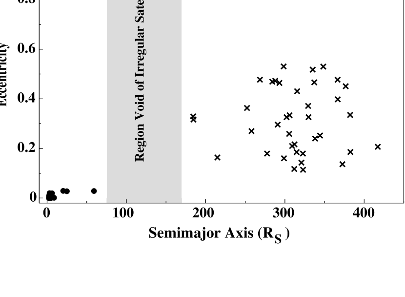
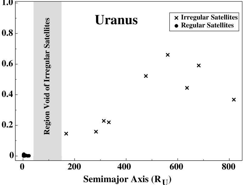
Figure 1: Satellite systems of the four giant planets. The $x-$axes show the semimajor axes of satellites in the units of the radii of their host planets.

Observations suggest the presence of similar void regions around all four giant planets. Table 1 and figure 1 show this in more detail. As seen from figure 1, satellite void regions also exist between the currently known irregular satellites of the giant planets. Theoretical studies have indicated that there may be two possible scenarios for the existence of such void regions; ejection from the system due to mutual interactions with other irregular satellites and, in the case of satellites that are the remnants of collisions, clustering around their parent bodies (Kuiper, 1956; Pollack, Burns, and Tauber, 1979; Kessler, 1981; Thomas et al., 1991; Krivov et al., 2002; Nesvorný et al., 2003; Nesvorný, Beaugé, and Dones, 2004; Beaugé and Nesvorný, 2007). The focus of this paper is, however, on the lack of irregular satellites in the boundary between regulars and irregulars. We are interested in understanding of why no irregular satellite exists between the outermost Galilean satellite and Jupiter’s innermost irregular one.

The lack of irregular satellites in the boundary between regulars and irregulars may be attributed to the distribution of the orbits of the latter bodies. Since irregular satellites appear to have been captured from heliocentric orbits, it may be natural to expect them to preferably have large semimajor axes, and therefore not to exist in close orbits. Proving this to be so would be an important contribution to the subject, but, unfortunately, none of the models of capture is sufficiently specific to be used in this way. The N-body capture model of Nesvorný, Vokrouhlický, and Morbidelli (2007) does roughly match the distribution of irregular satellites of some planets, but not of Jupiter. In this paper, we examine the possibility of a dynamical origin for the existence of this satellite-void boundary region.

The origin of irregular satellites and the mechanisms of their capture remain unknown. The high values of the orbital inclinations and eccentricities of these objects imply an origin outside the primordial circumplanetary disk from which the regular satellites of giant planets were formed. It is believed that irregular satellites were formed elsewhere and were captured in their current orbits (Kuiper, 1956; Pollack, Burns, and Tauber, 1979; Nesvorný et al., 2003; Nesvorný, Beaugé, and Dones, 2004; Jewitt and Haghighipour, 2007).

The capture of irregular satellites might have occurred during and/or after the formation of the regular satellites of the giant planets. Given that the latter objects are formed through the collisional growth of small bodies in a circumplanetary disk (Canup and Ward, 2002; Mosqueira and Estrada, 2003a, b; Estrada and Mosqueira, 2006), the orbits of captured irregulars might have been altered by perturbations from these objects during their formation and after they are fully formed. In the case of Jovian irregulars, the migrations of Ganymede and Callisto (Tittemore and Wisdom, 1988, 1989, 1990; Goldreich and Tremaine, 1980; Canup and Ward, 2002) have also had significant effects on the dynamics of irregular satellites.

In this paper we study the dynamics and stability of irregular satellites between Callisto and Themisto. We present the details of our model in §2, and an analysis of the results in §3. Section 4 concludes this study by reviewing our study and discussing its limitations.

2 Numerical Simulations

We numerically integrated the orbits of several hundred test particles in a region interior to the orbit of Themisto, the innermost Jovian irregular satellite. We assumed that the regular satellites of Jupiter were fully formed and studied the perturbative effects of the Galilean satellites on the dynamics of small objects in their vicinities. We considered a system consisting of Jupiter, the Galilean satellites, and 500 test particles uniformly distributed between 30 and 80 Jupiter-radii. The initial orbital elements of the test particles were chosen in a systematic way as explained below.

1) At the beginning of each simulation, test particles were placed in orbits with semimajor axes starting at $30{R_{J}}$ and increasing in increments of 0.1$R_{J}$.

2) For each initial value of the semimajor axis of a test particle $(a_{p})$, the initial orbital eccentricity $(e_{p})$ was chosen to be 0, 0.2, 0.4, and 0.6. This choice of orbital eccentricity matches the range of the current values of the orbital eccentricities of Jovian irregulars, as shown in figure 1.

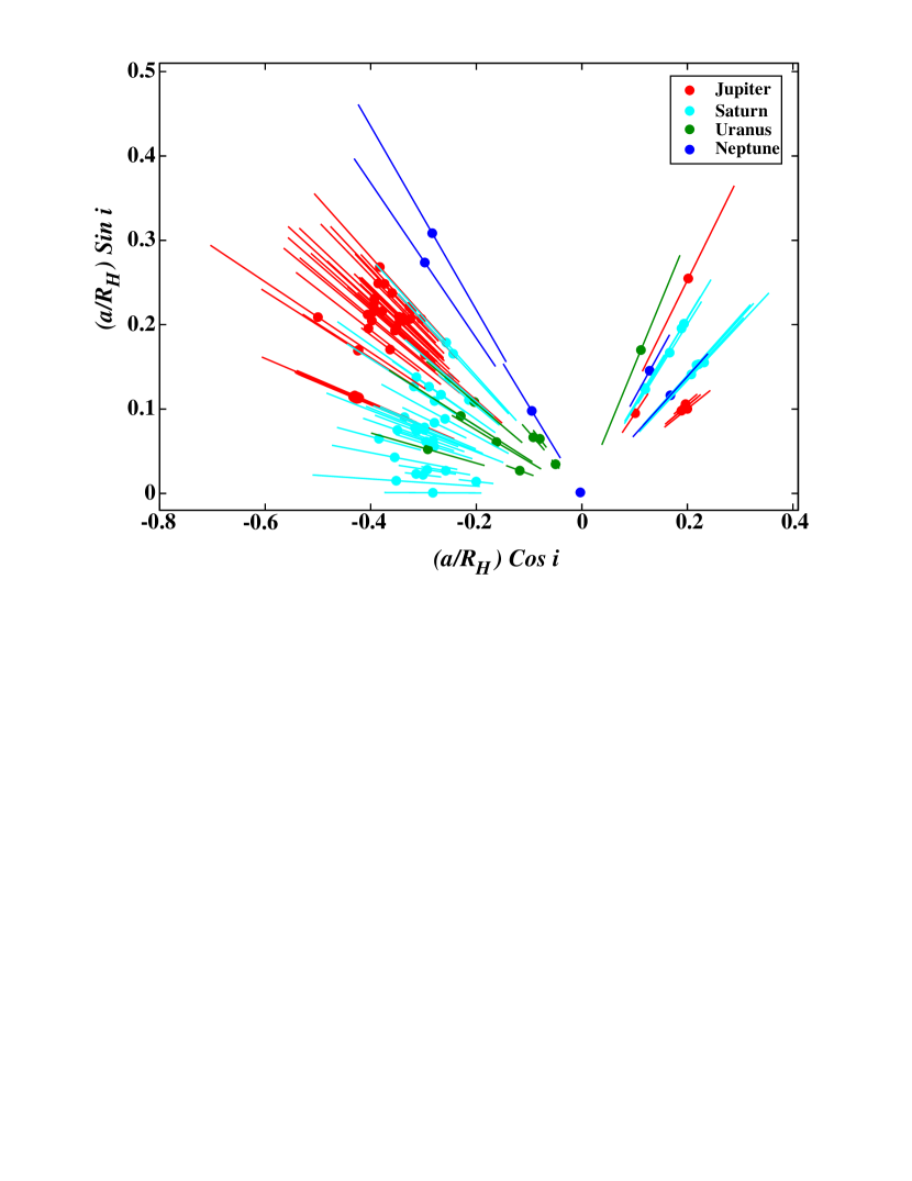
Figure 2: Distribution of irregular satellites around the four giant planets. The quantities on the axes represent the semimajor axis of a satellite, $a$, the Hill radius of its host planet, $R_{H}$, and the satellite’s orbital inclination, $i$. The distance of each satellite from the origin of the graph is equivalent to its semimajor axis, and its radial excursion (the distance from its periastron to apastron) is given by the length of its associated line. The angle between this line and the horizontal axis is equal to satellite’s orbital inclination.

3) The initial orbital inclinations of test particles $(i_{p})$ were varied between $0^{\circ}$ and $180^{\circ}$ in steps of $20^{\circ}$. As shown by figure 2, irregular satellites are absent at inclinations between $55^{\circ}$ and $130^{\circ}$ due to perturbations resulting from the Kozai resonance (Kozai, 1962; Hamilton and Burn, 1991; Carruba et al., 2002; Nesvorný et al., 2003). In choosing the initial orbital inclinations of these objects, we made a conservative assumption and considered the region of the influence of Kozai resonance to be between $60^{\circ}$ and $120^{\circ}$. We did not integrate the orbits of the test particles for ${i_{p}}={80^{\circ}},{100^{\circ}}$ and $120^{\circ}$.

4) Since we were interested in studying the effects of the perturbations of regular satellites on the variations of the orbital eccentricities and inclinations of test particles, we considered the initial values of the argument of the periastron, longitude of the ascending node, and the mean-anomaly of each test particle to be zero. This is an assumption that was made solely for the purpose of minimizing the initial-value effects.

We numerically integrated the orbits of the Galilean satellites and the test particles of our system for different values of the test particles’ orbital eccentricities and inclinations. Simulations were carried out for 10 Myr using the N-body integration package MERCURY (Chambers, 1999). Since the objects of our interest are close to Jupiter, we neglected the perturbation of the Sun and considered Jupiter to be the central massive object of the system. This assumption is consistent with the findings of Hamilton and Krivov (1997), who have shown that around a giant planet with a Hill radius $R_{H}$, the gravitational force of the Sun destabilizes the orbit of prograde irregular satellite at distances larger than 0.53$R_{H}$ and those of the retrograde irregulars at distances beyond 0.69$R_{H}$. For Jupiter, these values translate to 389$R_{J}$ for prograde irregulars and 507$R_{J}$ for retrograde ones. We carried out all integrations with respect to Jupiter with timesteps equal to the 1/20 of the orbital period of Io.

3 Discussion and Analysis of the Results

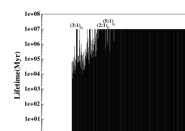
Figure 4: Lifetimes of the test particles of figure 3. Both systems are coplanar. In the upper graph ${e_{p}}=0$, and in the lower graph ${e_{p}}=0.2$. The locations of mean-motion resonances with Ganymede and Callisto are also shown.

To study the relation between the orbital parameters of test particles and their stability, we determined the lifetime of each particle, considering ejection from the system and collision with other bodies. We considered a particle to be ejected when it reached a distance of 2000$R_{J}$ or larger from the center of Jupiter. A collision, on the other hand, occurred when the distance between a particle and a Galilean satellite became smaller than ${R_{GH}}={a_{GS}}{({M_{GS}}/3{M_{J}})^{1/3}}$, or the particle’s closest distance to the center of Jupiter became smaller than Jupiter’s radius. Here, $a_{GS}$ and $M_{GS}$ represent the semimajor axis and mass of a Galilean satellite, and $M_{J}$ is the mass of Jupiter. Figure 3 shows the graphs of the test particles’ lifetimes in terms of their initial semimajor axes for particles in two coplanar systems. The graph at the top corresponds to particles initially in circular orbits, and the one at the bottom shows the lifetimes of particles with initial eccentricities of 0.2. The positions and lifetimes of the regular satellites of Jupiter and the orbit of Themisto are also shown. As shown by the upper graph, test particles in circular orbits are mostly stable (for the duration of integrations) except for a few that are close to Callisto. The region of stability, however, becomes smaller (instability progresses toward larger distances) in simulations in which the initial eccentricities of test particles are larger. This can be seen more clearly in figure 4 where from the graphs of figure 3, only the regions between $30{R_{J}}$ and $80{R_{J}}$ are shown. The islands of instability, corresponding to mean-motion resonances with Callisto (indicated by the subscript C) and Ganymede (indicated by the subscript G) are also shown.

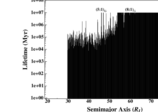
Figure 5: Lifetimes of test particles in a system in which ${e_{p}}=0.4$ and ${i_{p}}=20^{\circ}$. The locations of mean-motion resonances with Ganymede and Callisto are also shown. As shown here, compared with the systems of figures 3 and 4, as the initial eccentricities of test particle increase, their region of instability extends to farther distances.

The migration of unstable regions to larger distances in systems where test particles were initially in eccentric orbits was observed in all our simulations. Figure 5 shows another example of such a system. In this figure, the lifetimes of test particles with initial eccentricities of 0.4 and initial inclinations of 20^∘ are shown. The unstable region extends to distances beyond their corresponding regions in figures 3 and 4.

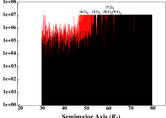
Figure 6: Lifetimes of test particles with initial eccentricities of ${e_{p}}=0.4$ and orbital inclinations of ${i_{p}}=40^{\circ}$ (black) and ${i_{p}}=140^{\circ}$ (red). As shown here, particles in retrograde orbits (red) are more stable. The locations of mean-motion resonances with Ganymede and Callisto are also shown.

We also simulated the dynamics of test particles having orbital inclinations larger than 90^∘ (retrograde orbits). As shown by figure 2, the number of irregular satellites is larger at these angles implying that retrograde orbits have longer lifetimes (Hamilton and Krivov, 1997; Touma and Wisdom, 1998; Nesvorný et al., 2003). Our simulations also show that retrograde orbits are more stable than their corresponding prograde ones. Figure 6 shows this for two sets of test particles. The particles in black correspond to a system in which ${e_{p}}=0.4$ and ${i_{p}}=40^{\circ}$. The particles in red correspond to a system with similar orbital eccentricity, but with ${i_{p}}=140^{\circ}$. As expected, the particles on retrograde orbits are more stable and maintain their orbits for longer times.

The fact that the region of instability of test particles, having a given semimajor axis, expands by increasing the initial values of their orbital eccentricities can be attributed to the interactions of these particles with Jupiter’s regular satellites. Given that the orbits of Jovian regulars are almost circular, an eccentric orbit for a test particle implies a smaller periastron distance for this object, and consequently a closer approach to the system’s regular moons. Instability occurs when the perturbative effects of regular satellites disturb the motion of a test particle in its close approach. The outer boundaries of the influence zones of the Galilean satellites (Table 2) mark the extent of these perturbations. Particles with periastron distances beyond these boundaries, i.e., ${a_{p}}(1-{e_{p}})>({a_{GS}}+3{R_{GH}})$, will more likely have longer lifetimes.

Figure 7 shows the boundaries of the stable and unstable test particles for all Galilean satellites. The initial positions of test particles with $({e_{p}},{i_{p}})$ equal to (0,0), (0.2,0), (0.4,40), (0.4,140), (0.6,60), and (0.6,120), are also shown. The stable particles are shown in black and unstable ones are in red. As shown here, particles with higher initial orbital eccentricities penetrate the influence zones of Ganymede and Callisto, and their orbits become unstable. Figure 7 also shows that for particles with similar semimajor axes, the boundary between the stable and unstable regions extends to larger distances by increasing the particle’s eccentricity. For instance, when interacting with Callisto, in order for a particle to maintain stability, ${a_{p}}(1-{e_{p}})>28{R_{J}}$. However, for particles in figure 5, where ${e_{p}}=0.2$, this implies that the region of instability extends to at least $35{R_{J}}$.

Although for a given semimajor axis, the boundary of stable and unstable regions expands with increasing orbital eccentricities of the test particles, for a given value of this eccentricity, the destabilizing effects of the Galilean satellites reach to larger semimajor axis, beyond their influence zones. At such distances, although the perturbative effects of Galileans are small they may, in the long term, disturb the motions of other objects and render their orbits unstable. An example of such instability can be seen in figure 7 for $({e_{p}},{i_{p}})=(0.2,0),(0.4,40),(0.6,60)$ and also in figure 5, where the unstable region extends to approximately $46{R_{J}}$. These results also imply that in simulations similar to those shown in figure 3, the region of instability may migrate outward if the integrations are continued to much larger times beyond 10 Myr.

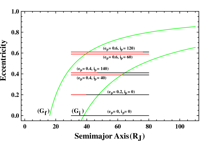
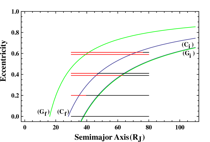
Figure 8: Top: curves of the constant-periastron (boundaries of stable and unstable regions) of a test particle for which the constant values are equal to the distance of the outer boundary of the influence zone of Ganymede before its migration (the curve denoted by ${\rm G}_{\rm i}$) and after it migrates to its present orbit (the curve denoted by ${\rm G}_{\rm f}$). The stable (black) and unstable (red) test particles in the region between $30{R_{J}}$ and $80{R_{J}}$ are also shown. Bottom: Similar constant-periastron curves as in the above for Ganymede and Callisto. Note that, because the pre-migration semimajor axes of Ganymede and Callisto are close to one another ($30{R_{J}}$ and $35{R_{J}}$, respectively), it seems as though the two curves ${\rm G}_{\rm i}$ and ${\rm C}_{\rm i}$ in the bottom graph are in contact with one another. The stable and unstable test particle are also similar to the top graph.

Ganymede and Callisto may have undergone inward radial migrations after their formation (Goldreich and Tremaine, 1980; Canup and Ward, 2002). As noted by Canup and Ward (2002), Ganymede might have started its inward migration from a distance not larger than approximately $30{R_{J}}$, and Callisto might have migrated inward from approximately $35{R_{J}}$. The perturbative effects of these satellites have, therefore, influenced a larger region beyond their current influence zones. Figure 8 shows this in more detail. In this figure, the top graph shows the boundary of stable and unstable test particles for Ganymede before and after its radial migration. The bottom graph in figure 8 shows the similar curves for both Ganymede and Callisto. The influence zones of these two satellites were initially larger, implying that many small objects might have been destabilized during the migrations phase.

Even when including radial migration, the influence zones of Ganymede and Callisto do not cover the entire region between Callisto and Themisto. For the 10 Myr integration time presented here, the interactions with Ganymede and Callisto do not seem to account for the lack of irregular satellites at distances beyond 60$R_{J}$. Since at such distances, the perturbative effects of Ganymede and Callisto are weaker, extension of integrations to longer times may reveal that this region is indeed unstable. We also speculate that the lack of irregular satellites at such distances is the result of a clearing process that has occurred during the formation of the Jovian regular moons. As shown by Canup and Ward (2002), and by Mosqueira and Estrada (2003a, b), regular satellites of giant planets might have formed through the collisional growth of smaller objects (satellitesimals) in a circumplanetary disk. Similar to the formation of terrestrial planets in our solar system, where the mutual collisions of planetesimals around the Sun resulted in the formation of many protoplanetary objects, satellitesimals might have also collided and formed a disk of protosatellite bodies around giant planets. The interaction between protosatellites and smaller bodies in such circumplanetary disks could have destabilized the orbits of many of these objects and resulted in their collisions, accretion by protosatellites, and/or ejection from the system. The final locations of surviving irregular satellites at smaller distances were then limited by the outer boundary of a region that included the influence zones of regular satellites, as well as the above-mentioned dynamically cleared area. For Jovian irregulars, a conservative assumption places this limit at $76{R_{J}}$ on the curve of constant-periastron of Themisto. Figure 9 shows this limit in light blue. At larger distances, on the other hand, the stability of irregular satellites is governed by the perturbation from the Sun. The boundaries of the Sun-perturbed regions have been shown in figure 9 as curves of constant-apastron, with the constant value equal to 0.53$R_{JH}$ for prograde irregulars and 0.69$R_{JH}$ for retrograde ones (Hamilton and Krivov, 1997). The quantity $R_{JH}$ is the Hill radius of Jupiter. It is important to note that the values of the eccentricities and semimajor axes of the irregular satellites in figure 9 were obtained from the documentation on solar system dynamics published by JPL, in which the orbital parameters of a body have their mean values and, unlike the test particles in our simulations, their angular elements are non-zero. This implies that although figure 9 portrays a qualitatively reliable picture of the stability of the Jovian irregular satellites, a more detailed mapping could be obtained by assuming zero values for the initial angular elements of irregular satellites and simulating their stability for 10 Myr.

4 Summary and Concluding Remarks

We numerically integrated the orbits of 500 test particles for different values of their orbital elements, in a region between $30{R_{J}}$ and $80{R_{J}}$. Our integrations indicated that the long-term stability of these objects is affected by the values of their initial periastron distances. For given values of their semimajor axes, the region of instability of test particles extended to larger distances as the initial values of their orbital eccentricities were increased.

Our numerical simulations also showed that, except at large distances from the outer boundaries of the influence zones of Ganymede and Callisto, the lack of irregular satellites between Callisto and Themisto can be attributed to the instability of test particles caused by their interactions with the two outermost Galilean satellites. At larger distances (e.g., between $\sim 40{R_{J}}$ to 80$R_{J}$ for particles in circular orbits, and between $\sim 60{R_{J}}$ to 80$R_{J}$ for particles with initial orbital eccentricities of 0.4), however, the perturbations of Galilean satellites do not seem to be able to account for the instability of small bodies. A possible explanation is that their instability is the result of interactions with Jovian satellitesimals and protosatellites during the formation of Jupiter’s regular moons.

Because the test particles in our simulations were initially close to Jupiter, we neglected the effect of solar perturbations. As shown by Hamilton and Krivov (1997), for Jupiter, the shortest critical distance beyond which the perturbation from the Sun cannot be neglected corresponds to prograde orbits and is equal to 389$R_{J}$. In our simulations, the outermost test particle was placed well inside this region at 80$R_{J}$. It is important to note that, although the effects of solar perturbations on our test particles are small and will not cause orbital instability, they may, in the long term, create noticeable changes in the orbital evolution of test particles. For instance, solar perturbations may enhance the perturbative effects of regular satellites in increasing the orbital eccentricity of test particles and result in their capture in Kozai resonance. More numerical simulations are needed to explore these effects.

As mentioned in §2, different non-zero angular elements may in fact affect the stability of individual test particles. However, the analysis of the stability of the system, as obtained from our numerical simulations, portrays a picture of the dynamical characteristics of the test particles that, in general, is also applicable to Jovian irregular satellite systems with other initial angular variables.

The applicability of our results and the extension of our analysis to the satellite-void boundary regions around other giant planets may be limited due to fact that their satellite systems are different from that of Jupiter. Although the above-mentioned dynamical-clearing process can still account for the instability of many small objects around these planets, numerical simulations, similar to those presented here, are necessary to understand the dynamical characteristics of their small bodies in more detail.

Figure 3: Lifetimes of test particles in a coplanar system with ${e_{p}}=0$ (top) and ${e_{p}}=0.2$ (bottom). The locations of the regular satellites of Jupiter and Themisto are also shown.

Figure 7: Boundaries of stable and unstable regions of a test particle (i.e., curves of constant-periastron for which the constant value is equal to the distance of the outer boundary of the influence zones of the Galilean satellites). The black and red horizontal lines represent the initial semimajor axes of test particles between $30{R_{J}}$ and $80{R_{J}}$ for different values of their orbital eccentricities and inclinations. The particles in black maintained their orbits for the duration of integration (10 Myr) whereas the particles in red became unstable.

Figure 9: Graph of the region of the stability of Jovian irregular satellites. Prograde satellites are in purple and retrograde ones are in orange. The inner boundary of this region, shown in light blue, corresponds to the curve of constant-periastron of Themisto. Its outer boundary, shown in purple for prograde irregulars and in orange for retrograde ones, is a curve for constant-apastron equal to the largest distance a Jovian irregular satellite can travel before its orbit becomes unstable by solar perturbation. The curves of constant-periastron corresponding to the influence zones of Ganymede and Callisto, as explained in figure 8, and the stable (black) and unstable (red) test particles, within the region of $30{R_{J}}$ to $80{R_{J}}$, are also shown.

Table 1: Irregular satellite-void regions around giant planets

Satellite	Void Region (Planet Radii)
Jupiter	30-80
Saturn	59-184
Uranus	23-167
Neptune	223-635

Table 2: Influence zones of the Galilean Satellites.

Satellite	Semimajor Axis $(R_{J})$	Inner boundary $(R_{J})$	Outer boundary $(R_{J})$
Io	5.8	5.4	6.3
Europa	9.3	8.7	9.8
Ganymede	14.8	13.5	16.1
Callisto	26.0	24.0	28.0

References

- Beaugé, Nesvorný and Dones (2006) Beaugé, C., Nesvorný, D., and Dones, L., 2006, AJ, 131, 2299
- Beaugé and Nesvorný (2007) Beaugé, C., and Nesvorný, D., 2007, AJ, 133, 2537
- Canup and Ward (2002) Canup, R. M., and Ward, W. R., 2002, AJ, 124, 3404
- Carruba et al. (2002) Carruba, V., Burns, J. A., Nicholson, P. D., and Gladman, B., 2002, Icarus, 158, 434
- Chambers (1999) Chambers, J. E., 1999, MNRAS, 304, 793
- Douskos, Kalantonis and Markellos (2007) Douskos, C., Kalantonis, V., and Markellos, P., 2007, Astrophys. Space. Sci., 310, 245
- Estrada and Mosqueira (2006) Estrada, P. R., and Mosqueira, I., 2006, Icarus, 181, 486
- Goldreich and Tremaine (1980) Goldreich, P., and Tremaine, S., 1980, ApJ, 241, 425
- Hamilton and Burn (1991) Hamilton, D. P., and Burns, J. A., 1991, Icarus, 92, 118
- Hamilton and Krivov (1997) Hamilton, D. P., and Krivov, A. V., 1997, Icarus, 128, 241
- Jewitt and Haghighipour (2007) Jewitt, D., and Haghighipour, N. 2007, ARA&A, 45, 261
- Kessler (1981) Kessler, D. J., 1981, Icarus, 48, 39
- Krivov et al. (2002) Krivov, A. V., Wardinski, I., Spahn, F., Kruger, H. and Grun, E., 2002, Icarus 157, 436
- Kozai (1962) Kozai, Y., 1962, AJ, 67, 591
- Kuiper (1956) Kuiper, G. P., 1956, Vistas in Astronomy, 2, 1631
- Mosqueira and Estrada (2003a) Mosqueira, I., and Estrada, P. R., 2003, Icarus, 163, 198
- Mosqueira and Estrada (2003b) Mosqueira, I., and Estrada, P. R., 2003, Icarus, 163, 232
- Nesvorný et al. (2003) Nesvorný, D., Alvarellos, J. L. A., Dones, L., and Levison, H. F., 2003, AJ, 126, 398
- Nesvorný, Beaugé, and Dones (2004) Nesvorný, D., Beaugé, C., and Dones, L., 2004, AJ, 127, 1768
- Nesvorný, Vokrouhlický, and Morbidelli (2007) Nesvorný, D., Vokrouhlický, D., and Morbidelli, A., 2007, AJ, 133, 1962
- Pollack, Burns, and Tauber (1979) Pollack, J. B., Burns, J. A., Tauber, M. E., 1979, Icarus, 37, 587
- Saha and Tremaine (1993) Saha, P., and Tremaine, S., 1993, Icarus, 106, 549
- Sheppard and Jewitt (2003) Sheppard, S. S., and Jewitt, D., 2003, Nature, 423, 261
- Thomas et al. (1991) Thomas, P., Veverka, J., and Helfenstein, P., 1991, J. Geophys. Res., 96, 19253
- Tittemore and Wisdom (1988) Tittemore, W. C., and Wisdom, J., 1988, Icarus, 74, 172
- Tittemore and Wisdom (1989) Tittemore, W. C., and Wisdom, J., 1989, Icarus, 78, 63
- Tittemore and Wisdom (1990) Tittemore, W. C., and Wisdom, J., 1990, Icarus, 85, 394
- Touma and Wisdom (1998) Touma, J., and Wisdom, J., 1998, AJ, 115, 1653