The Araucaria Project: The Local Group Galaxy WLM - Distance and Metallicity from Quantitative Spectroscopy of Blue Supergiants

Abstract

The quantitative analysis of low resolution spectra of A and B supergiants is used to determine a distance modulus of 24.99$\,\pm\,$0.10 mag (995$\,\pm\,$46 Kpc) to the Local Group galaxy WLM. The analysis yields stellar effective temperatures and gravities, which provide a distance through the Flux weighted Gravity–Luminosity Relationship (fglr). Our distance is 0.07 mag larger than the most recent results based on Cepheids and the tip of the RGB. This difference is within the 1$\displaystyle\sigma$ overlap of the typical uncertainties quoted in these photometric investigations. In addition, non-LTE spectral synthesis of the rich metal line spectra (mostly iron, chromium and titanium) of the A supergiants is carried out, which allows the determination of stellar metallicities. An average metallicity of -0.87$\,\pm\,$0.06 dex with respect to solar metallicity is found.

1 Introduction

WLM is one of the faintest dwarf irregular galaxies ($M_{B}\cong-14$), located in an isolated part of the Local Group. Detailed photometric studies have shown that it consists of a young population concentrated in a disk and an old extended metal poor halo (Ferraro et al., 1989; Minniti & Zijlstra, 1997; Dolphin, 2000; Rejkuba et al., 2000; McConnachie et al., 2005). The color of the red giant branch of the old population indicates a metallicity of [Fe/H] = -1.45 dex representing the end of the first star formation episode. On the other hand, the metallicity of the young population is somewhat ambiguous. While measurements from a number of Hii regions (Skillman et al., 1989; Hodge & Miller, 1995; Lee et al., 2005) yielded a low nebular oxygen abundance of [O/H] = -0.8 dex, a detailed high resolution spectroscopic study of an A-type supergiant (Venn et al., 2003) obtained [O/H] = -0.2 dex indicating a large discrepancy between stellar and nebular chemical composition. On the other hand, Bresolin et al. (2006) in their low resolution (5 Å) spectroscopic survey for supergiants in WLM studied three early B supergiants and found an average value of [O/H] = -0.8 dex comparable with the Hii regions.

The spectroscopic sample gathered in the survey by Bresolin et al. (2006) also contained high signal-to-noise data of several late B and A supergiants (B5-A7) of luminosity class Ia and II. These objects with their rich spectra of metal lines (mostly iron, titanium, chromium) are ideal for a further investigation of stellar metallicity. However, at the time of the publication of this work the density of metal lines in the optical spectra together with the low spectral resolution did not allow for a determination of stellar parameters using the standard analysis techniques applied for the early-type B supergiants. Recently, this situation has changed. Kudritzki et al. (2008, hereafter K08) in their study of the Sculptor spiral galaxy NGC 300 at a distance of 1.9 Mpc developed a new technique to quantitatively analyze low resolution spectra of A supergiants with respect to stellar parameters and metallicity. This technique makes use of the Balmer jump and the Balmer lines to obtain effective temperature and gravity and determines metallicity from a $\chi^{2}$-minimization of observed and theoretical spectra in selected spectral windows. It can now be applied to the data set obtained by Bresolin et al. (2006) and allows for a more comprehensive straightforward spectroscopic study of the metallicity of the young stellar population in WLM.

The distance to WLM has been determined from photometric studies of the old stellar population using the tip of the red giant branch (TRGB), the horizontal branch (HB) and full color-magnitude diagrams, yielding distance moduli between 24.7 and 24.95 mag (see Rizzi et al., 2007, and references above). The most recent comprehensive multi-color survey for Cepheids by Gieren et al. (2008), including J- and K-band photometry, found a distance modulus of 24.92 mag with a very small random error of 0.04 mag and a systematic error of 0.05 mag. These authors determined an average interstellar reddening E(B-V)=0.08 mag, significantly larger than the Galactic foreground reddening and, thus, relevant for the derived distance. Under such circumstances, an independent distance and reddening determination using the young stellar population is ideal for verifying photometrically based distances.

Such an independent distance determination can be provided through the quantitative spectral analysis of the B and A supergiants. Kudritzki et al. (2003) and K08 have shown that a tight correlation exists between the absolute bolometric magnitude and the flux weighted gravity $g/T_{eff}^{4}$. This relationship is predicted by stellar evolution theory and allows distance determinations with a precision comparable to Cepheids.

In this paper, we will carry out a spectral analysis of the low resolution optical spectra of 8 late B and A supergiants (B5-A7) observed by Bresolin et al. (2006) to determine stellar temperatures, gravities, luminosities, masses and metallicities. For the analysis we will use the basic concept introduced by K08, however, in a modified form. We will present a new numerical fit algorithm based on an empirical application of the Karhunen-Loève expansion usually referred to as Principal Component Analysis, which allows for an automated analysis of a large number of objects using large comprehensive grids of model atmosphere spectra. We will then combine the results with those obtained by Bresolin et al. (2006) for the early-type B supergiants and determine an independent distance using the flux-weighted gravity luminosity relationship, fglr. This will be the first distance determination using this new distance determination method.

The paper is organized as follows. After a brief description of the observations in §2 we present the modified analysis method in §3. In §4, we test our method by comparing with the results obtained in a previous detailed high resolution study for one of our targets. The results of the analysis, i.e. the derived $T_{\!\mbox{\scriptsize\em eff}}$, $log~{}g$, metallicity, E(B-V), radius, luminosity and mass, are given in §5. The distance determination using the fglr is carried out in §6 and §7 will present a discussion of all the results.

2 Observations

The spectroscopic observations were obtained with the Focal Reducer and Low Dispersion Spectrograph 2 (FORS2, Appenzeller et al., 1998) at the ESO Very Large Telescope in multi-object spectroscopy mode in one night of good seeing conditions (better than 0.7 arcsec) on 2003 July 28 as part of the Auracaria Project (Gieren et al., 2005). The total exposure time is 4500s and the air mass during the observations was smaller than 1.07. The spectral resolution is approximately 5 Å and the spectral coverage extends over 2500 Å centered at 4500 Å for most of our targets. The spectra were also flux calibrated so that spectral energy distributions, in particular the Balmer jump, can be used to constrain the stellar parameters. The observational data set has been described by Bresolin et al. (2006). The paper also contains finding charts, coordinates, photometry (V, I from the Las Campanas 1.3m telescope, see Pietrzyński et al., 2007), radial velocities and spectral types. Of the 19 confirmed supergiants found with spectral types ranging from late O to G, 8 were of spectral type B5 to A7. The S/N per pixel for these objects is between 40 to 120, sufficient for our quantitative analysis. This sample listed in Table 1 and selected for this work. The target designation follows the nomenclature in Bresolin et al. (2006). Note that we consider only stars of their A set because of the significantly better S/N.

Along with the broad band photometry in the aforementioned reference, we also use B-, V-, R- and I-band data published by Massey et al. (2007) to constrain the interstellar reddening E(B-V), as well as J- and K-band photometry from Gieren et al. (2008). The IR photometry, available only for some stars, is compiled in Table 2.

Prior to the quantitative spectral analysis, we carefully explore the dataset available for each star, to identify spectral regions showing signs of contamination due to imperfect sky subtraction, nearby cosmic rays, and similar other observational effects. These regions are masked out and not used in the analysis.

3 Quantitative spectral analysis

As explained in K08 the principal difficulty in the analysis of low resolution spectra of A supergiants lies in the simultaneous determination of effective temperature and metallicity. The classic method based on the use of ionization equilibria does not work, since the required lines from the neutral species (Mg I, Fe I, …) are in general very weak and disappear at low resolution within noise and the blends of spectral lines. While one could use the information from the stronger lines, which define the spectral type, and a calibration of spectral type with effective temperature, such a relationship is metallicity dependent, which requires the simultaneous and independent determination of metallicity.

K08 were able to solve this problem by using the Balmer jump as an independent temperature indicator in addition to the Balmer lines, which can be used as a measure of gravity, and to the rich metal line spectrum, which yielded the metallicity through a $\chi^{2}$-minimization comparing selected windows of the observed spectra with very sophisticated non-LTE line formation calculations.

The methodology employed in the present work follows closely the ideas presented by K08, however with some significant modifications. While K08 constructed fit diagrams of the Balmer jump and the Balmer lines in the $T_{eff}$–$log~{}g$ plane through “by eye” fits of the observed line profiles and the spectral energy distribution (SED) and then determined the metallicity for the effective temperature and gravity at the intersection of the two fit curves. Here we have developed a completely automated numerical method, which finds the best fit of the model atmosphere synthetic spectra to the observed spectra. The advantages of this new method are obvious. It provides a more quantitative and objective way to obtain the fit and the automated procedure allows a quantitative analysis of a large number of spectra, which in the era of efficient multi-object spectrograph facilities is a very important aspect. We will describe the method in the subsections below.

3.1 Brief description of the model grid

The basis for the quantitative spectral analysis is the same comprehensive grid of line blanketed LTE model atmospheres and very detailed non-LTE line formation calculations used by K08. For a detailed description of the physics of the model atmosphere and line formation calculations see Przybilla et al. (2006).

Our grid of models covers a range of $\displaystyle 8300\leq T_{eff}\leq 15000$ K (with steps of 250 K and 500 K below and above 10⁴ K, respectively) and $\displaystyle 0.75\leq log~{}g\leq 2.60$ (with steps of 0.05 dex) in effective temperature and gravity with the following metallicities at each grid point, [Z] = $\log\left(\mathrm{Z/Z}\right)_{\odot}$: -1.30, -1.00, -0.85, -0.70, -0.60, -0.50, -0.40, -0.30, -0.15, 0.00, 0.15, 0.30. The quantity Z/Z_⊙ is the metallicity relative to the Sun. The solar abundances were taken from Grevesse & Sauval (1998), except for oxygen, which is from Asplund et al. (2004). Based on trend in the literature, a microturbulence of 8 ${\rm km}\>{\rm s}^{-1}\,$ is adopted for the low gravity models gradually changing to 4 ${\rm km}\>{\rm s}^{-1}\,$ at higher gravity. For further details we refer to K08.

This grid was primarily designed for the analysis of Ia and Ib luminosity class objects. Several of the WLM stars selected for the present work were classified by Bresolin et al. (2006) as luminosity class II. To consider these objects, we enlarged the grid with two new effective temperatures, 8100 and 7900 K, and extended to higher gravities all the models with $\displaystyle T_{eff}\leq 10^{4}$ K ($log~{}g\leq 2.75$ dex).

3.2 General methodology

The goal of the analysis is to determine for each star a set of four parameters $\{T_{eff}$, logg, [Z] and E(B-V)$\}$, for which the corresponding synthetic model spectrum best matches the observations. We have three data sets available: 1) normalized and rectified spectra, which will give line profile information for the Balmer and metal lines; 2) flux calibrated spectra providing information about the Balmer jump, and 3) broad band photometry which can be used for the construction of the observed long wavelength SED.

K08 have shown in detail how the theoretical spectral line profiles, the SED and the Balmer jump depend on temperature, gravity and metallicity. Generally speaking, the Balmer lines depend mostly on gravity, but show also a significant temperature dependence, whereas the Balmer jump depends mostly on temperature, but also on gravity. The dependence on metallicity of the Balmer lines and the Balmer jump is very weak. Using these properties, two different curves can be defined in the $T_{eff}$–$log~{}g$ plane, one being the locus of the models that reproduce the Balmer lines when the temperature is adopted, and, conversely, another tracing the locus of the models that reproduce the Balmer jump once the gravity is assumed. The intersection of these two curves yields the gravity and the temperature of the star observed. The classic method used by K08 is to construct these curves through a by-eye fit of the models to the observed data. In our new approach we have decided to use an automated numerical fit of the model spectra to the observed data.

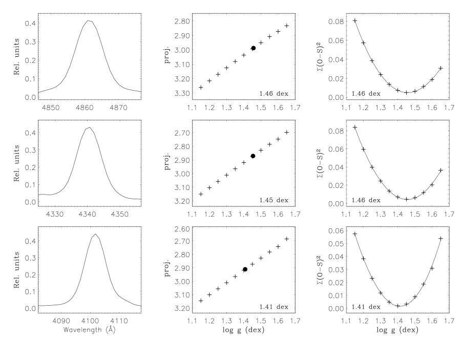
Figure 1: Determination of surface gravity. For illustration purposes, only three lines are presented. From top to bottom: H$\beta$, H$\gamma$ and H$\delta$. For each line, the first panel shows the base vector, the second one displays the projection of the models (crosses) and the observed spectrum (filled dot), and the third panel presents a solution by applying a minimum distance method (minimization of the quadratic differences, $\sum_{\lambda}\left(O_{\lambda}-S^{j}_{\lambda}\right)^{2}$ ) for comparison. The derived $log~{}g$ for each line is also included in each individual plot.

a) Our algorithm is iterative and begins with the fit of the Balmer lines. We start with a first value of $T_{eff}$ and [Z] and try to find the model gravity $log~{}g$ which best matches the shape of the observed Balmer profiles. For this purpose, we carry out a Principal Component Analysis (PCA) of the normalized model spectra in spectral windows around the Balmer lines. For a fixed $T_{eff}$ and [Z] we have n models with different gravities at each grid point (n varies from 20 to 32 depending on the grid point), each of them providing a set of normalized flux values S${}_{j}(\lambda)$ (where the index j runs over the n models) around a selected Balmer line. These model flux values define a matrix $\mathbf{A}$ (with elements A${}_{ij}\,=\,$S${}_{j}(\lambda)$, where i labels the wavelength points and j runs over the models with different $log~{}g$). Following the concept of PCA, we determine the eigenvalues and the eigenvectors of the covariance matrix $\mathrm{cov}\!\left(\mathbf{A}\right)$ (Deeming, 1964; Whitney, 1983) and identify the largest eigenvalue and its corresponding eigenvector as the principal component associated with the parameter $log~{}g$. Fig. 1 shows the typical eigenvectors $\mathbf{v}(\lambda)$ for three Balmer lines. As a consistency test we check that the cumulative percentage variance associated with this principal component is always above 95% in all cases, meaning that more than 95% of the information in the input data can be described by the principal component alone.

The projection of the model flux matrix $\mathbf{A}$ onto the eigenvector $\mathbf{v}$ allows us to define a relationship between the $log~{}g$ values of the models and their projections $\displaystyle\Phi(log~{}g)$, for each Balmer line

$$\sum_{\lambda}\mathrm{S}_{j}\left(\lambda\right)\,v\left(\lambda\right)\,=\,\Phi_{j}\,=\,\Phi\left(log~{}g\right)$$

which are also shown in Fig. 1. Projecting the observed normalized flux values $F_{\lambda}$ in each Balmer line spectral window onto the corresponding eigenvector yields an observed value, which can then be compared to $\Phi(log~{}g)$ to find the best gravity $log~{}g$ at the selected values of $T_{eff}$ and [Z]. Comparing the values obtained from different Balmer lines (we usually use H₁₀ to H_β) allows us to assign a mean value and an uncertainty $\omega$ to this determination of the best fitting gravity.

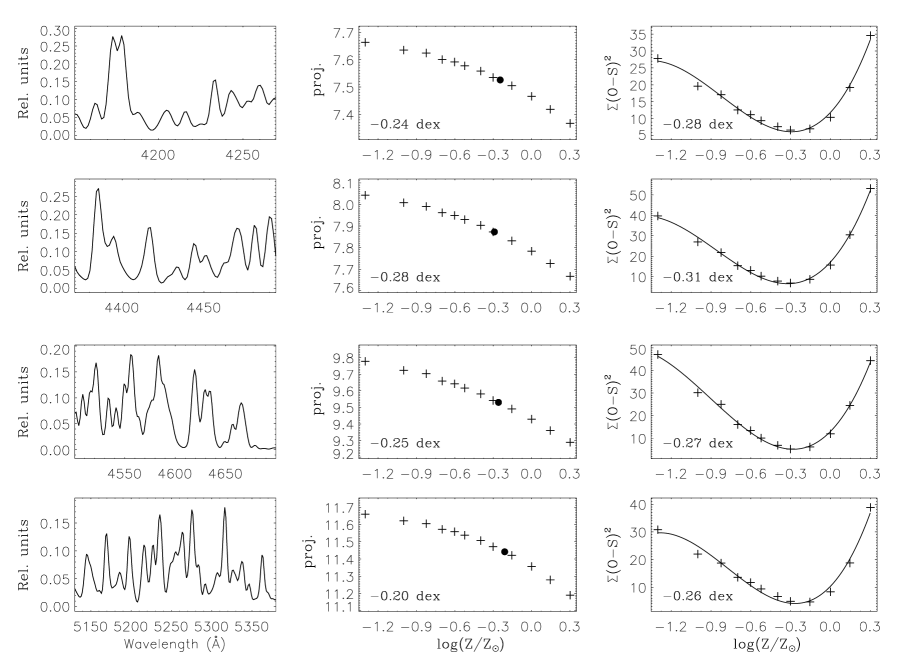
Figure 2: Metallicity determination. For illustration purposes, only four spectral windows are shown. For details about each individual panel, see previous figure.

b) Adopting this pair of $\left(T_{eff},\,log~{}g\right)$ we can now determine a new metallicity by defining spectral windows with many metal lines. Fig. 2 shows a typical example of different spectral windows and their corresponding PCA eigenvectors, this time determined with respect to metallicity [Z]. The projections $\Phi([Z])$ and the observed value are also shown. Using different spectral windows we can again assign an average value of [Z] and an uncertainty $\omega$. For this new [Z] we iterate the determination of $log~{}g$, but because of the weak dependence of the Balmer lines on metallicity changes are usually small.

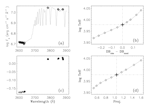
Figure 3: Determination of $T_{eff}$: (a) definition of the Balmer jump region; diamonds identified the wavelength points use to create the PCA base vector. (b) $T_{eff}$ determination based on the minimum difference between the observed and modeled Balmer jump measurements, with D${}_{\mathrm{B}}\,=\,<\log$F${}_{\lambda}^{\mathrm{pre}}>\,-\,<\log$F${}_{\lambda}^{\mathrm{post}}>\,$ following K08; the cross marks the derived temperature. (c) PCA base vector for the Balmer jump, and (d) projection of the models (hollow diamonds) and the observed Balmer area (cross).

c) In the previous steps we used Balmer and metal line profiles to obtain $log~{}g$ and [Z] (and their corresponding uncertainties) at a selected value of $T_{eff}$. Now we adopt these new values of $log~{}g$ and [Z] and use the observed SED around the Balmer jump to obtain a new value of $T_{eff}$. This is again done by PCA (but see below) as shown in Fig. 3. The model atmosphere SED corresponding to this $T_{eff}$, $log~{}g$ and [Z] is used to determine the reddening E(B-V) from a comparison ($\chi^{2}$-minimization) with the observed broad band photometry, adopting the extinction law by Cardelli et al. (1989), as well as $\displaystyle R_{v}=A_{V}/E(B-V)=3.1$. Since the region used to determine $T_{eff}$ could be affected by this extinction, we alternatively iterate the values of $T_{eff}$ and E(B-V) until convergence in both is reached, defining the best $T_{eff}$ and the best E(B-V). Unlike the cases of surface gravity and metallicity, the temperature is determined from a single feature, the Balmer jump. The uncertainty in $T_{eff}$ is thus given by our ability to effectively measure the Balmer jump, and not from temperature values derived from different spectral windows. In order to estimate this uncertainty, we proceed in the following way. Two values of the temperature are computed simultaneously, by using two different definitions of the Balmer jump (see Fig. 3). The first one (Fig. 3d) corresponds to the value derived from the application of the PCA base vector (shown in Fig. 3c), while the second value (Fig. 3b) is based on the Balmer jump index $D_{B}$ introduced by K08, $\displaystyle D_{B}=\langle\log(F_{\lambda}^{long})\rangle-\langle\log(F_{\lambda}^{short})\rangle$, where

$$\begin{array}[]{l}\langle\log(F_{\lambda}^{short})\rangle=\{\sum_{i=1}^{N}\log(F_{\lambda_{i}})\}/N,~{}3585\mathrm{\AA}\leq\lambda_{i}\leq 3627\mathrm{\AA}\quad\mathrm{,and}\\ \langle\log(F_{\lambda}^{long})\rangle=\{\log F_{3782\mathrm{\AA}}+\log F_{3814\mathrm{\AA}}+\log F_{3847\mathrm{\AA}}+\log F_{3876\mathrm{\AA}}\}/4\end{array}$$

In the case of $\displaystyle F_{\lambda}^{short}$, $N$ is the number of wavelength points considered for the mean. Note that in both cases, we are considering all the models in the grid for a given pair $\displaystyle\left(log~{}g,[Z]\right)$, as previously explained. In an ideal case, with infinite S/N, both values would be exactly the same. Once noise is present, there is a difference between both temperatures, that reflects how precisely the Balmer jump can be measured, defining therefore the uncertainty in temperature, $\displaystyle\Delta T_{eff}$.

Apart from this $\Delta T_{eff}$, the difference between the initially assumed temperature and the final derived value defines an error $\delta$, which can be assigned to the set of parameters $\displaystyle\{T_{eff},log~{}g,[Z],E\left(B-V\right)\}$. This $\delta$ can be interpreted as the distance between the guess temperature and the true $T_{eff}$, because of the weak dependence of the Balmer jump on gravity and metallicity.

We repeat the whole procedure (a, b, c) for different initial values of $T_{eff}$ and, thus, obtain a set of parameters $\pi_{i}\,=\,\{T_{eff},log~{}g,[Z],\mathrm{E}\left(\mathrm{B-V}\right)\}_{i}$ together with their corresponding weights $(\delta_{i},\omega_{i})$. The final solution $\Pi$ = $\{T_{eff}$, logg, [Z] and E(B-V)$\}$ is then obtained as a weighted mean

$$\Pi\,=\,\frac{\sum_{i}\,1/\delta^{2}_{i}\,\cdot\,1/\omega^{2}_{i}\,\cdot\,\pi_{i}}{\sum_{j}\,1/\delta^{2}_{j}\,\cdot\,1/\omega^{2}_{j}}$$

where the indexes $i,j$ run over all the individual solutions for the corresponding parameter ($T_{eff}$, logg, [Z] or E(B-V)). In a similar way, a formal error (uncertainty) is obtained from

$$(\Delta\>\Pi)^{2}\,=\,\frac{\sum_{i}\,1/\delta^{2}_{i}\,\cdot\,1/\omega^{2}_{i}\,\cdot\,(\pi_{i}-\Pi)^{2}}{\sum_{j}\,1/\delta^{2}_{j}\,\cdot\,1/\omega^{2}_{j}}$$

This analysis method can only be applied in those cases for which the Balmer jump region is observed. In some instances, due to the location of the star in the observed field and its spectrum on the detector, this area is not observed, and we have to rely on the normalized spectrum to obtain information about the effective temperature. In this situation as already discussed by K08, the relative strength of lines from different species can be used. If the star is hot enough to show He I lines (earlier than around A0), these can be used to constrain the temperature. The accuracy is usually comparable to that when the Balmer jump is used. If the star is cool enough (later than B9), the relative behavior of different metal lines (for example Ti II versus Fe II lines, or the strength of the Fe-Mg blend located at $\sim\,$5150 Å) could be used. To find the temperature, we then proceed in a similar way, defining several spectral windows in which these metal or helium lines are present, to construct the PCA eigenvectors (from the normalized synthetic spectra), but now with respect to temperature. There is an underlying assumption, though, when using this method: the adopted metallicity pattern. The implications of our adopted solar abundance pattern are discussed in Sect 3.4. Temperatures determined by this method have a somewhat larger uncertainty, related to the accuracy with which the metallicity can be determined.

Metallicity and microturbulence are closely related with respect to the values derived from any analysis. As discussed by K08, it is difficult to constraint microturbulence at such low spectral resolution, since lines from a given species, with very different strengths, are required. In consequence, as explained in §3.1, for each object, the microturbulence is given by the final ($T_{eff}$,$log~{}g$) pair. We will discuss in §3.4 the possible effects of the adopted relationship between the microturbulence and the ($T_{eff}$,$log~{}g$) values.

3.2.1 Uncertainties

The formal accuracy of the final solution depends primarily on the signal-to-noise ratio. Our experience shows that, for the low spectral resolution considered in this work, a minimum S/N$\sim$50 is required for the metallicity determination in order to keep the uncertainties in a tolerable range (see next section), while T_eff and $log~{}g$ determinations, both based on stronger features (the Balmer jump and the Balmer lines) can still be carried out at much lower, S/N$\sim$15.

The formal errors arising from the application of our algorithm, as previously defined, are rather small. Typically, surface gravity and metallicity can be constrained to better than 0.05 dex, while the effective temperature uncertainty results in a few K. To define more meaningful errors, we also consider the uncertainties derived for the model in the grid with parameters closest to the final solution, i.e., we use the $\omega$ values (defined above) obtained for the set $\displaystyle\{T_{eff},log~{}g,[Z]\}$ closest to the final solution. These provide an idea about how well the observations are reproduced by a single model.

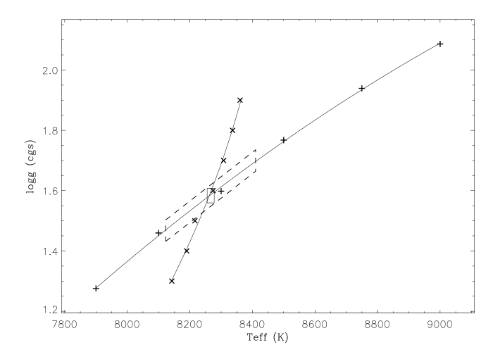
Figure 4: $T_{eff}$–$log~{}g$ diagram for star A14 of our sample. The solution provided by the algorithm is defined by the small box, while the solution obtained by the conventional method would be located at the intersection of the two $T_{eff}$–$log~{}g$ fit curves for the Balmer jump (x) and the Balmer lines (+). The dashed lines define the final uncertainties in the derived parameters.

The final errors quoted are obtained as a quadratic combination of these two sets of uncertainties. Typical values for these final errors result in $\sim$ 2–5% in temperature, $\sim$ 0.1–0.2 dex in surface gravity and $\sim$ 0.2–0.3 dex in metallicity. As an example, Fig. 4 shows the solution obtained for one of the stars in the sample, A14. The small box encloses the solution with the formal errors in the $T_{eff}$–logg plane. As can be seen this solution area agrees with the intersection of the conventional fit curves for the Balmer jump and the Balmer lines, with the difference of the solutions well below the resolution limit of both methods. The final adopted errors are represented by the dashed box.

With regard to the uncertainties in the flux weighted gravity, it must be noted that the errors in $log~{}g$ and $T_{eff}$ are correlated (see Fig. 4), which reduces the uncertainties in $log~{}g_{\mathrm{F}}$ in most cases. The reader is referred to K08 for a detailed discussion on this topic.

3.2.2 Goodness-of-fit assessment

With the final set of parameters known for each star, it is useful to evaluate the fitness of each final solution, with the goal of identifying problems not detected in the analysis. Given a pair observation–final model $\displaystyle\left(O_{\lambda},M_{\lambda}\right)$, we define the residuals of a spectral window with $\displaystyle n_{i}$ wavelength points as

$$r_{i}\left(M_{\lambda},O_{\lambda}\right)=\frac{1}{n_{i}}\left[\sum_{j=1}^{n_{p}}\left(\frac{O_{j}-M_{j}}{M_{j}}\right)^{2}\right]^{1/2}$$

The fitness $\displaystyle R\left(\Pi\right)$ of a parameter $\Pi$ is given by the sum of these relative residuals $\displaystyle r_{i}$ over all the spectral windows considered in the determination of the corresponding parameter (as described above), weighted by the (normalized) S/N of each individual window

$$R\left(\Pi\right)\>=\>\sum_{i=1}^{n_{w}}{r_{i}\hat{s_{i}}}\qquad\mathrm{,with}\qquad\hat{s_{i}}=\frac{\mathrm{S/N}_{i}}{\sum_{k}{\mathrm{S/N}_{k}}}$$

In the case of the surface gravity and metallicity, the normalized spectra are used to calculate the fitness. For the effective temperature, the flux calibrated data and the synthetic SEDs are considered to evaluate the fitness when the Balmer jump is observed. If it is not observed the normalized spectra are used.

Alternatively, we could define the fitness for each window as

$$q_{i}\left(M_{\lambda},O_{\lambda}\right)=\frac{1}{n_{i}}\sum_{j=1}^{n_{p}}\left(\frac{\log(O_{j}/M_{j})}{\log(1+\epsilon)}\right)$$

where $\displaystyle\epsilon$ is the error allowed in the fitting (tolerance), defined as $\displaystyle\epsilon=\mathrm{S/N}^{-1}$. The global fitness, for each parameter individually, is given by the sum over all the windows, in this case without weighting by the S/N since its effect is already accounted for with the tolerance. This second fitness evaluator has the advantage of containing additional information in its sign, with a positive/negative value reflecting whether the corresponding parameter is over or under-estimated. This fitness definition is particularly useful to detect variations in the goodness-of-fit from star to star.

We define the global fitness of the model with respect to the observation, $\displaystyle R\left(M_{\lambda},O_{\lambda}\right)$, as the sum of the individual fitness values of each parameter, $\displaystyle R\left(\Pi\right)\!$. From the definitions, it is clear that the smaller the absolute value, the fitter the model. Fitness values corresponding to the final solutions are presented in Table 3, and they will be used in the following sections to discuss the results.

3.3 Consistency tests

We performed a number of simple tests to check the analysis algorithm. In all the following cases, we emulated the observed spectra by degrading the models to a resolution of 5 Å (FWHM) and re-sampling them to 1.32 Å (the spectral resolution and dispersion provided by FORS2 when equipped with the 600B grism). Note that these tests are meant to check our ability to reproduce known input parameters.

First, we verified that, for any given model in the grid, we were able to recover almost exactly its parameters. In a second step, we created a number of models with parameters within the limits of the grid, but without any corresponding model in the grid. Three different sets of $\displaystyle T_{eff}$–logg, representatives of a late B, an early A and a mid A supergiants were considered, for four different metallicities. In all cases, we were able to recover the parameters to better than 1% in effective temperature (based on the Balmer jump), 0.02 dex in surface gravity and 0.03 dex in metallicity. These two tests were carried out without considering noise, since they were intended to probe the ability of our algorithm to recover known parameters, without any influence from external sources.

A third set of tests was performed to check the effect of noise on the determination of metallicity, and hence to evaluate the minimum S/N required for (meaningful) metallicity determinations. We selected a number of models in the grid representative again of the different spectral groups, degraded them to different S/N (100, 50, 30 and 15) and carried out a metallicity analysis. For each model and each S/N value, we did 100 independent trials. The results for the early A-type case are presented in Fig. 5 (the results are very similar for all the other $T_{eff}$–logg pairs considered). The first two rows correspond to $\left[\mathrm{Z}\right]=0.00$ dex, while the other two rows are for $\left[\mathrm{Z}\right]=-0.85$ dex. Each single plot displays the relative frequency of occurrence versus the difference between the input and recovered metallicities, presenting also the sigma of the distribution. Since this sigma only describes the dispersion introduced by the noise, the global uncertainty obtained in a generic analysis would be larger, once the effects of the uncertainties in the other parameters (temperature and gravity) are accounted for. As a general recipe, a maximum $\sigma_{S/N}\sim 0.10$ dex at a fixed pair of $T_{eff}$ and $logg$ would be required in order to have a final global uncertainty $\sigma\sim 0.20$ dex.

Clearly, the minimum S/N depends on the metallicity: the higher the $\left[\mathrm{Z}\right]$, the stronger the lines, hence the lower the S/N required to detect them. At the same time, it also depends to some extent on the spectral type; for a given metallicity, cool mid A-types (A1 to A3) present stronger metal features (as well as a higher line density) than late B-/early A-types (B5 to A0). From Fig. 5, it is possible to identify a minimum S/N$\sim$50, in particular at low metallicities, to meet the requirement of a global metallicity uncertainty around 0.2 dex.

3.4 Dependence of the results on hidden parameters

In order to keep the task of creating such a huge model grid manageable, only three parameters (the most important ones, $T_{eff}$, $logg$ and [Z]) are explored so far. In the following we want to discuss some of the possible implications regarding how the models are calculated.

As previously stated, metallicity and microturbulence are coupled in any analysis. Aimed at exploring the effect that our assumption about microturbulence $\xi$ (given for a pair $T_{eff}$-logg) could have on the results, we calculated a small set of models with different values of $\xi$ (but the same $T_{eff}$, $logg$, [Z] considered for the grid), and analyzed them in the same manner as the observations. For a variation of $\xi$ of $\pm$2 ${\rm km}\>{\rm s}^{-1}\,$(which is the typical dispersion obtained in high resolution analyses of these type of objects, for a given luminosity class) we found an error of less than 1%, 0.01 dex and 0.07 dex for effective temperature, surface gravity and metallicity, respectively. As expected, both $T_{eff}$ and logg are unaffected by a change in microturbulence, and the larger effect is produced in the metallicity. Here we want to stress again that we are not dealing with individual lines, which certainly could present large variations with $\xi$ (like for example Mg II 4481 Å), but with all the spectral lines at once (or with as many of them as possible); the use of the whole spectrum weights the effect of the turbulence differently, reducing its impact on the derived global metallicity. This is, on the other hand, a warning sign for the use of small sections of the spectrum (at low resolution) to determine individual elemental abundances, which would be seriously hampered by the unknown $\xi$.

We proceeded in a similar way in order to evaluate the impact of our assumption of a solar abundance pattern. We calculated a set of models for which the ratio of the $\alpha$-elements to Fe-group elements relative to the solar reference vary, with [$\alpha$/Fe] = $\pm\,$0.15, $\pm\,$0.30 dex (note that by definition, the value used in the grid is [$\alpha$/Fe] = 0.0 dex). The maximum change in effective temperature (based on the Balmer jump) and surface gravity due to these changes in relative abundances is less than 1% and 0.01 dex respectively. The difference goes up to 6% in temperature when using the normalized spectrum instead of the Balmer jump. This result is not surprising since in this case, $T_{eff}$ is based on the relative strength of different species, in particular of Ti II to Fe II lines, which depends on the relative abundances as well as on the temperature. As a byproduct, this exploratory study allowed us to refine the limits for some of the spectral windows considered in the determination of metallicities, allowing also to identify features that are produced mainly by Fe-group elements (Fe, Ni, Cr, …) and, conversely, features produced by $\alpha$-elements (in particular Ti). This will be used in the future to evaluate the possibility of extracting information from the spectra not only for the global metallicity but also for the relative abundances of some prominent species.

3.5 Comments on individual stars

In this section we present a brief discussion of the analysis of some of the targets.

• A4: the Balmer jump region was not observed for this star, therefore we have to use the normalized spectrum to estimate $T_{eff}$ from metal lines (the star is too cool to present He lines). In this situation, $T_{eff}$ is coupled to [Z], the well know problem of the spectral type–metallicity degeneracy. Due to the combination of the low metallicity and the relatively low S/N, the errors in [Z] and $T_{eff}$ are relatively large.

• A5 and A17: the Balmer jump is missing for both stars. Fortunately, they are hot enough to present He I lines, and can be used to constraint $T_{eff}$. Note that both stars have S/N above 50, which greatly improves the situation with respect to the two previous cases.

• A6: the analysis of this star is problematic. While the determination of $T_{\!\mbox{\scriptsize\em eff}}$ and $log~{}g$ using the Balmer jump and the Balmer lines is straightforward and results in fitness values similar as for the other stars, the determination of [Z] is not. The metallicity is not well defined, as is indicated by the high values of $\displaystyle R\left([Z]\right)$ and $\displaystyle Q\left([Z]\right)$ compared to the other stars. Moreover, the high value of [Z]=-0.15 dex is puzzling. We note that the spectral type found by Bresolin et al. (2006) based on the relative strength of Ca II H and K lines is A7, suggesting a significantly cooler temperature than the one obtained from the Balmer jump. While there are other examples of A supergiants where the Ca II related spectral types do not match $T_{\!\mbox{\scriptsize\em eff}}$ (see discussion of star A16) mostly because of the contribution by interstellar lines (note that E(B-V) of A6 is 0.29 mag), we have tried to obtain a spectral fit at cooler temperatures ($T_{eff}=8100$ K, $log~{}g=1.50$ dex) with a metallicity [Z]=-0.7 dex more in line with the other stars. At these parameters, the Balmer lines are reproduced well, but the fit of the Balmer jump is unacceptable as indicated by the fitness values in Table 3. In addition, the fitnesses $R\left([Z]\right)$ and $Q\left([Z]\right)$ are only marginally improved and still significantly worse than the fits for the other stars. The value for E(B-V) at this cool temperature is 0.27 mag, only slightly lower than before.

  The problem described above might be caused by stellar multiplicity. We have tried to emulate the observables (Balmer jump, normalized spectrum and broad band photometry) by combining two models, one hot to reproduce the Balmer jump and one cool to produce the rich metal spectrum and the Balmer lines. However, it has been impossible to find a combination of models to fit everything. Also, the star does not show signs of companions in archival WFPC2/HST images. Even more puzzling is the fact that all the different photometric measurements considered, from B- to K-band (including WFPC2/HST photometry in filters F555W and F814W taken from Holtzman et al. 2006) are satisfactorily reproduced with a single model solution, invoking high reddening.

  Another possibility is that we are dealing with a completely different type of star with just the photometric and (partial) spectroscopic appearance of an A supergiant. The only solution that comes to our mind is a low mass star, for instance in post-RGB or post-AGB phase, in the Galaxy. Venn et al. (2003) have already discussed this possibility and found that this is rather unlikely. Indeed, if we assume the typical mass of 0.5 M_⊙ for these objects, then with $log~{}g=1.95$ dex and $T_{eff}=8750$ K, we obtain $log~{}L/L_{\odot}=2.9$ or $M_{\mathrm{bol}}=-2.5$ mag, with which, an apparent magnitude of $m_{\mathrm{bol}}=18.9$ mag would put the object at a distance of 190 Kpc, certainly outside the Galaxy. We also note that A6 has a radial velocity typical for a WLM member (Bresolin et al., 2006).

  At this point, we consider the metallicity of A6 obtained in our analysis as unreliable. We will include the object in our discussion of the fglr and of interstellar reddening, but will regard it uncertain.

• A14: this star has been previously studied by Venn et al. (2003), to which these authors referred as WLM-15. In their analysis, Venn et al. (2003) found a significant discrepancy between the oxygen abundance of the star and the abundances obtained from H II regions. We compare our results with those of Venn et al. (2003) in the following section. Unfortunately, our wavelength coverage does not include O lines, therefore it is not possible to carry out an independent analysis of the oxygen abundance.

• A16: the spectral type classification by Bresolin et al. (2006), based on the Ca II lines, is not consistent with the spectrum, nor with the results of the analysis (see below). There is at least another well known case for which this also happens. The Galactic star HD 12953, the standard A1 Ia in the MK system, would be classified as an A3 based on the strength of its Ca II lines, as already discussed by Evans & Howarth (2003). Unlike the case of A6, a completely consistent solution can be found.

4 Comparison with high resolution spectroscopy

One of the stars in our sample, A14, was previously studied by Venn et al. (2003, hereafter V03). These authors obtained a high resolution optical spectrum with UVES at the VLT (R$\sim$32000), and subsequently analyzed it using model atmosphere techniques similar to the ones employed here. This offers the possibility of a comparison with our low resolution work.

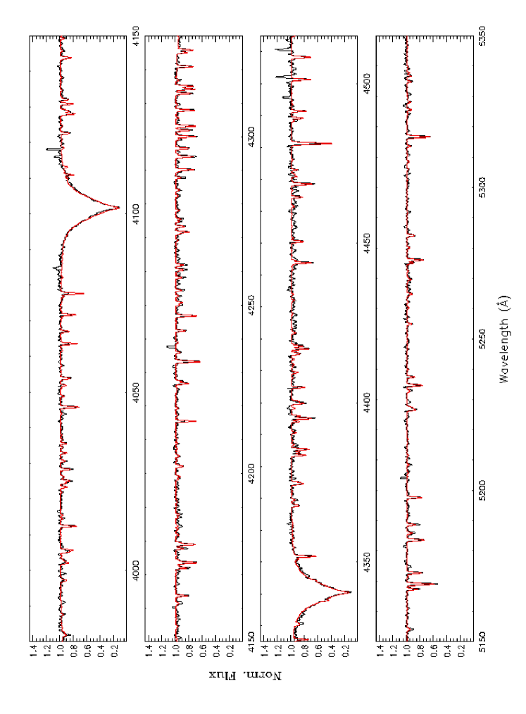
Figure 6: UVES/VLT (R=32000) spectrum of WLM-A14 compared with our solution (red) obtained from the analysis of low-resolution FORS2/VLT (R$\sim$1000) spectrum.

For the fundamental parameters, $T_{eff}$ and logg, V03 obtained 8300$\,\pm\,$200 K and 1.60$\,\pm\,$0.10 dex, while our solution is 8270$\,\pm\,$145 K and 1.60$\,\pm\,$0.12 dex. The agreement is very good. Worth noticing is the fact that the effective temperature of V03 is based on the Mg ionization equilibrium, while ours is based on the Balmer jump. With respect to the chemical abundances, the high resolution work is far superior in the sense that it can provide individual elemental abundances, while we derive a global metallicity. In order to compare with our result, we used V03’s individual abundances of Fe, Ti, Sc and Cr (and our solar references) and calculated a mean [Z] value of -0.44$\,\pm\,$0.13 dex (the latter number is the standard deviation of this weighted mean). Note that neither O nor N lines available to V03 are covered in our observed spectral range, thus we decided not to include them to compute [Z]. Within the uncertainties, this value is in good agreement with our derived value of -0.50$\,\pm\,$0.19 dex. In fact, this good concordance can be seen in Fig. 6, were we show the UVES spectrum of A14 and a model with the parameters resulting from our low resolution analysis, convolved with the appropriate UVES instrumental profile and rotational velocity.

While the comparison can only be done for one star, the close agreement found is certainly very encouraging, in particular given the relatively low metallicity of the object. This agreement is also in consonance with the result presented by Bresolin et al. (2006) for the early B-type supergiant A9 in the same galaxy.

5 Results

The stellar parameters obtained in our work are summarized in Table 4. In the following we discuss metallicity, interstellar extinction and stellar parameters.

5.1 Metallicities

The metallicity of the 6 BA stars in our sample range (excluding A6) from $\left[\mathrm{Z}\right]=-0.5$ to $-1.0$ dex. The weighted mean metallicity, is $\left[\mathrm{Z}\right]=-0.87\,\pm\,0.06$ dex, where the uncertainty is given by the standard deviation of the sample. This value compares well with the results of Bresolin et al. (2006), based on the $\alpha$-element content of three early B-type supergiants, with weighted mean of $\left[\mathrm{O/H}\right]=-0.86\,\pm\,0.07$ dex. It also agrees with the oxygen abundances obtained from H II regions (Lee et al., 2005). This agreement indicates that WLM’s young stellar population while metal poor exhibits an abundance pattern very similar to the Sun (at least with respect to the most relevant species, like O, Fe or Ti).

It seems that A14’s metallicity is an outlier, being 0.26 dex above the mean, which is a bit larger than the individual uncertainties we are claiming in our analyses. As discussed above, our low resolution result is consistent with the high resolution analysis by Venn et al. (2003). The difference with respect to the rest of our sample, along with the abnormally high oxygen abundance derived by Venn et al. (2003) could indicate that the star has a peculiar history. We note that K08 in their study of NGC 300 have found two similar outliers not representing the expected metallicity at their galactocentric distance. They expressed that the idea of homogeneous metallicity might be naive. Excluding A14 from the weighted mean results in only a slight change to $\left[\mathrm{Z}\right]=-0.89\,\pm\,0.07$ dex.

Combining the results of our sample and the early B-type supergiants from Bresolin et al. (2006), there is no evidence of a metallicity dependence of the young stellar population with the spatial location in the galaxy (see Fig. 11).

5.2 Extinction

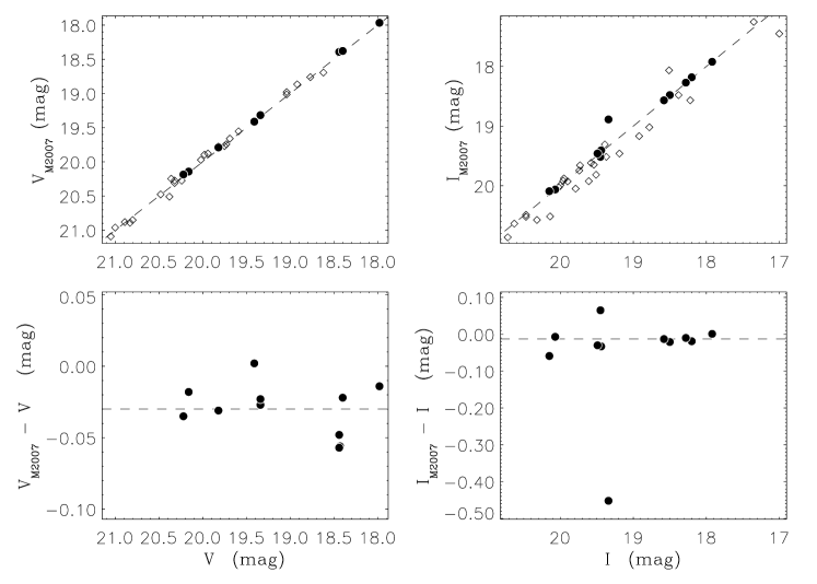
Figure 7: Comparison of photometric measurements. First row: V- and I-band photometric data from Bresolin et al. (2006) and Massey et al. (2007, M2007 subindex), for a total number of 35 stars in common (diamonds). The stars analyzed in this work, and the three early B-type supergiants of Bresolin et al. (2006) are represented by filled circles. The 1:1 relationship is represented by the dashed line. Second row: considering only the 11 stars analyzed in our work, we find a mean difference in the zero point calibration of $-0.03\pm 0.02$ mag and $-0.013\pm 0.030$ mag in V and I respectively. The star A17, not considered in the I-band mean, presents a difference with respect to our reference value of almost -0.5 mag.

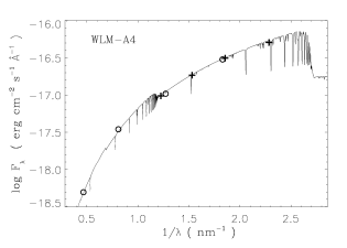
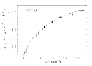
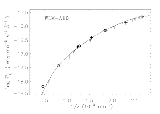
Figure 10: Synthetic reddened SEDs and photometric measurements for different stars in our WLM combined sample. Circles correspond to V and I photometric values from Bresolin et al. (2006) as well as J and Ks photometry from Gieren et al. (2008), and crosses stand for Massey et al. (2007) B,V,R and I-band data.

Reddening values were determined using Johnson V-band and Cousins I-band photometry from Bresolin et al. (2006) (see also Pietrzyński et al., 2007), along with B-V and V-R colors from Massey et al. (2007). V- and I-band data for the stars in common in these papers are shown in Fig. 7. For our sample of 11 B- and A-type supergiant stars (represented by filled dots in the figure) we obtain a difference in the zero points of $-0.03\pm 0.02$ mag and $-0.013\pm 0.030$ mag in V and I respectively, with the magnitudes from the first reference being fainter in both filters. Note that the star A17 was not considered in the I-band mean since it presents a large difference of almost -0.5 mag between both datasets. Using multi-epoch photometry (around 100 epochs, spanning over 2 yr), Bresolin et al. (2006) did not detect variability, beyond the observational scatter, for any of our targets. It is thus unlikely that the discrepancy in A17 I-band magnitudes is related to variability. In the case of the early B-type supergiant A9, its B-band magnitude is not consistent with all the other photometric measurements (see the corresponding plot in Fig. 10). In both cases, we did not take these values into account for the determination of the corresponding extinctions for the stars.

For four of the stars in the sample (A4, A6, A9, and A10), we also have IR J- and K-band data from Gieren et al. (2008).

The individual reddening values are presented in Table 4, and some examples comparing the reddened synthetic SEDs with the photometry are shown in Fig. 10. Individual reddening values range from 0.03 to 0.12 mag, with the extreme case of 0.29 mag for A6. Excluding this object, the mean reddening of the BA sample is 0.07$\,\pm\,$0.01 mag, or 0.08$\,\pm\,$0.01 mag when considering also the three early B-type supergiants. This mean value is higher than the characteristic foreground value of E(B-V)=0.037 mag (Schlegel et al., 1998), indicating that our stars suffer from internal (WLM produced) reddening. Our mean value is in agreement with the recent result by Gieren et al. (2008) based on multi-wavelength observations of Cepheids. These authors find a mean characteristic reddening of $0.082\pm 0.02$ mag.

With regard to A6, we note that a very high reddening value is derived for both the high temperature and the low temperature solution (discussed in Sect. 3.5). This means that the star suffers three times the mean reddening. A6 could be spatially associated with, or close enough to, one of the high column density H I areas identified by Kepley et al. (2007), in particular the region identified by these authors as the handle of the hook, extending north of the C1 H$\alpha$ complex of Hodge & Miller (1995). However, two of the three early B-type supergiants, A9 and A10, seem to be also spatially related to high column density H I regions, but they do not present such extreme reddening. We cannot discard, however, the possibility of a patchy ISM on small scales, and comparable cases of high reddening have also been found by K08 in NGC 300.

5.3 Masses, radii and luminosities

Once the fundamental parameters $T_{eff}$ and $log~{}g$ are known, it is possible to derive the distance dependent quantities by adopting a distance to WLM. In the next section, we will derive a distance to the galaxy based on the Flux weighted Gravity–Luminosity Relationship, FGLR, of blue supergiant stars (Kudritzki et al., 2003). For the purposes of this section, we adopt that distance, $\left(m-M\right)_{0}=24.99\pm 0.10$ mag, without any further explanation, delaying its derivation to the next section.

Using this distance, the apparent bolometric magnitudes can be converted to absolute bolometric magnitudes, and luminosities. From the luminosities and the effective temperatures, we compute the radii. With surface gravities and radii, it is then possible to derive (spectroscopic) masses. All these quantities are summarized in Table 5. To estimate their uncertainties, we propagate the uncertainties in the fundamental parameters.

From the luminosities, we can also derive stellar masses using theoretical evolutionary models (see Fig. 8). For this purpose, we use the mass-luminosity relationships presented by K08. In particular, we selected K08’s fits to SMC metallicity models from Maeder & Meynet (2001) and Meynet & Maeder (2005) that take into account rotation. These evolutionary masses are given in the last column of Table 5. The uncertainties of the spectroscopic masses take into account uncertainties in luminosities, gravities and radii. The uncertainties in evolutionary masses account only for the uncertainties in the derived luminosities and are much smaller. They are, however, affected by the systematic uncertainties of evolutionary tracks. Fig. 9a shows the comparison of evolutionary and spectroscopic masses, including the objects in NGC 300 studied by K08. Given the typical spectroscopic mass errors of $\pm 0.1$ to $0.2$ dex, we conclude that we have agreement between the two types of mass determinations. However, there is an indication that the spectroscopic masses are systematically smaller than evolutionary masses for high luminosities (above $M_{\mathrm{bol}}\sim-8$ mag, see Fig. 9b). We will discuss this in section 6.1.

From the direct inspection of the HRD and the masses given in Table 5, we conclude that the BA stars of our sample were born with masses in the range of 8 to 20 M_⊙, with the early B supergiants evolved from slightly more massive progenitors between $\sim$25 to 50 M_⊙. This is in agreement with the results found by K08 for NGC 300, who explain the difference of the masses as a selection effect.

6 Flux weighted gravity–luminosity relationship and distance to WLM

Kudritzki et al. (2003, see also K08) revealed the existence of a tight correlation between the flux weighted gravity, $g_{\mathrm{F}}=g/T_{\mathrm{eff}}^{4}$, and the luminosity of BA supergiant stars. This relationship is supported by the predictions of evolutionary models. Very briefly, the physical reason behind this is that during their evolution from the Main Sequence, massive stars with masses below $\sim 60\,\mathrm{M}_{\odot}$ will evolve at almost constant luminosity and, due to the short timescale and the low mass loss rates, constant mass. In this case, the luminosity of the star is correlated with the flux weighted gravity.

K08 have found a relation between the absolute bolometric magnitude and the flux weighted gravity of the form

$$M_{\mathrm{bol}}=\mathrm{a}\left(\log g_{\mathrm{F}}-1.5\right)+\mathrm{b}$$ (1)

with their present best values of the coefficients a and b derived from a large sample of supergiants combining spectroscopic results obtained for 8 different galaxies. These coefficients are given in Table 6. We also include the values obtained by K08 for only the supergiants in NGC 300, to give an idea of the uncertainties involved in calibrating this relationship.

The supergiants in WLM show a tight fglr when plotted in apparent bolometric magnitudes (in Fig. 12). This can now be used to determine a distance. Following K08, we fit an expression of the form

$$m_{\mathrm{bol}}=\mathrm{a}\left(\log g_{\mathrm{F}}-1.5\right)+\mathrm{b}$$

This fit is shown in Fig 12 by the solid line, and the values for a and b are given in Table 6 as well. With only ten stars the slope is somewhat uncertain, thus, we prefer to fix the slope to the value obtained by K08 for their large sample. We then recalculate the fit with this fixed slope (dashed line; the new value for the coefficient b is also presented in Table 6). The difference in b with respect to K08 then yields a first determination of the distance modulus, $\mu=\left(m-M\right)_{0}$, for which we obtain $\mu=24.99$ mag.

If we fix the slope to K08’s fglr for NGC 300 stars only, and compare again, we derive $\mu=25.06$ mag. This can be interpreted as an estimate of the possible systematic uncertainties to be about 0.06 mag.

The statistical uncertainty of the distance modulus is given by

$$\sigma^{2}=\frac{1}{n\left(n-1\right)}\sum_{i=1}^{n}\frac{\left(M_{\mathrm{bol},i}-M^{\mathrm{FGLR}}_{\mathrm{bol},i}\right)^{2}}{\widehat{\sigma}_{i}^{2}}$$

where $\displaystyle n$ is the number of WLM stars, $\displaystyle M^{\mathrm{FGLR}}_{\mathrm{bol},i}$ is obtained from Eq. 1 evaluated at the corresponding observed $\displaystyle g_{\mathrm{F},i}$, $\displaystyle M_{\mathrm{bol},i}$ is the apparent bolometric magnitude m_bol,i corrected by the derived distance modulus $\mu$, and $\widehat{\sigma}_{i}=\sigma_{i}/\sum_{j}\sigma_{j}$, with $\displaystyle\sigma_{i}^{2}=\sigma_{m_{\mathrm{bol}}}^{2}+a^{2}\sigma_{\log g_{\mathrm{F}}}^{2}$ the individual uncertainties in m_bol, accounting for the uncertainty in the BC, in the extinction and in the observed photometric errors, as well as the uncertainties in the flux weighted gravity. We obtain a statistical uncertainty associated with the distance modulus of $0.10$ mag.

An alternative way to determine the distance modulus is to minimize the residuals in magnitudes once the stars are shifted to a particular distance, i.e. we determine the value of $\mu$ that minimizes

$$S^{2}\!\left(\mu\right)=\frac{1}{n\left(n-1\right)}\sum_{i=1}^{n}\frac{\left(m_{\mathrm{bol},i}-\mu-M^{\mathrm{FGLR}}_{\mathrm{bol},i}\right)^{2}}{\widehat{\sigma}_{i}^{2}}$$

For this second method, the uncertainty in the distance determination is given by the square root of the minimized residuals.

The distances derived by both methods are in excellent agreement. This is a consequence of the fact that the slope of the relationship defined by the WLM stars is very close to the slopes found by K08 (see Table6). Fig. 13 presents the final distance corrected fglr for the WLM stars (filled circles), together with all the objects used by K08 to calibrate the relationship. This figure also includes K08’s fglr fit used to calculate the distance to WLM. As can be seen in this figure, the agreement is very good.

Finally, we would like to point out that the solution used for A6 (cool or hot model) has little effect on the derived distance, since the values of the flux weighted gravity are very similar in both cases, and in any case, a change in the flux weighted gravity is correspondingly accompanied by changes in the bolometric correction and extinction (relatively minor in this case), in such a way that the star moves along the relationship. The physical reason behind this behavior of $g_{\mathrm{F}}$ has been extensively discussed by K08, to which the reader is referred for further insights.

6.1 WLM FGLR: empirical versus theoretical relationships and metallicity dependence

In Fig. 14 we show the observed fglr for WLM compared with the prediction of stellar evolution. We have chosen the stellar evolution fglrs for solar and SMC metallicity using evolutionary tracks by Meynet & Maeder (2003), and Maeder & Meynet (2001) and Meynet & Maeder (2005), which include the effects of stellar rotation with initial rotational velocities of 300 ${\rm km}\>{\rm s}^{-1}\,$(for the related mass-luminosity relationships and the parameterization of the evolutionary fglrs see K08).

We note that for low luminosity and high flux-weighted gravity ($log~{}g_{\mathrm{F}}>1.6,\,M_{\mathrm{bol}}<-8$ mag) there is good agreement. However, towards lower gravities and higher luminosities the stellar evolution fglrs show a strong curvature and start to differ from the result of the spectral analysis. The effect is stronger for SMC metallicity ([Z]=-0.7), which is close to the average metallicity we have determined for the young stellar population in WLM. An indication of a similar discrepancy has already been noted by K08 (see their Fig. 27 and the corresponding discussion).

This discrepancy seems to be equivalent to a discrepancy between stellar evolutionary and spectroscopic mass at high luminosities (see Fig. 9). Note that (see K08, Eq.(29))

$$g_{\mathrm{F}}=gT_{\mathrm{eff,4}}^{-4}\propto MR^{-2}T_{\mathrm{eff}}^{-4}\propto ML^{-1}$$

and, in consequence, smaller spectroscopic masses result in a fglr shifted towards smaller flux weighted gravities. Thus, one reason for the discrepancy could be a systematic underestimate of stellar gravities by the spectral analysis at the high luminosity end of the fglr. We realize that the most discrepant objects in Fig. 9 and Fig. 14 are early B-type supergiants, which where analyzed with a different stellar atmosphere code. On the other hand, K08 had a much larger sample of supergiants available and did not find a systematic difference between high luminosity early B-types and BA-types.

Another possibility might be the effects of rotation on the evolutionary tracks. K08 noticed that tracks without rotation result in fglrs shifted towards higher gravities because the mass-to-light ratio is larger. Thus, tracks with even higher initial rotation than considered here may result in fglrs in better agreement with the observations. However, such increase in rotational velocity will not be supported by recent studies of LMC and SMC Main Sequence B stars, progenitors of BA supergiants, showing projected rotational velocities below 200 ${\rm km}\>{\rm s}^{-1}\,$ (see for example Hunter et al., 2008).

Finally, it is also important to discuss a possible metallicity dependence of the fglr. Except for the very high luminosity end, the relative difference between the evolutionary fglrs for [Z]=0.0 and [Z]=-0.7 is very small. This difference is mostly caused by the effects of mass-loss, which are stronger at higher metallicity and higher luminosity. The fact that we obtain a distance consistent with the TRGB and Cepheid studies of WLM using the fglr calibration by K08, which is based on objects mostly with LMC metallicity, supports the conclusion that metallicity effects are not important. Future work on supergiants in other metal poor galaxies will very likely help to clarify the situation.

7 Conclusions

The primary goal of this work has been to determine the distance to WLM using a new spectroscopic method, the fglr. The distance modulus obtained, 24.99$\pm$0.10 mag, compares well with recent determinations, based on purely photometric methods. Rizzi et al. (2007) found 24.93$\pm$0.04 mag from the TRGB (see also Pietrzyński et al., 2007, and references in Sect. 1) and the multi-wavelength study of Cepheids by Gieren et al. (2008) yielded 24.924$\pm$0.04$\pm$0.04 mag (statistical and systematic errors). With only 10 stars available for our study, the statistical uncertainty is larger than the ones claimed by the photometric studies. However, this could certainly be improved with a larger sample of objects. Our study also confirms that the young population of WLM suffers from significant extinction, higher than the foreground value. This is another example where the accurate measurement of intrinsic extinction turns out to be important for the determination of distances. It is the advantage of the spectroscopic method presented here that it yields reddening and extinction for the individual targets.

We have also determined stellar metallicities and found an average value of [Z]=-0.87$\,\pm\,$0.06 dex, in good agreement with previous H II region studies. The fact that the TRGB and fglr distances agree at this low metallicity indicates that metallicity effects are very likely small for the fglr  method.

Stellar evolution calculations can be used to determine a theoretical fglr, which can then be compared with observations. We find good agreement at low luminosities independent of metallicity assumptions for the theoretical relationship, but disagreement at higher luminosities with the theoretical fglr, which are more important for the low metallicity. Assuming higher initial rotational velocities, which would enhance mass-loss and rotational mixing, might be a way to solve this discrepancy. These higher rotational rates are not supported by recent studies of the progenitors of these objects in the Magellanic Clouds.

Finally, our results for A14 (aka WLM-15) are in good agreement with the results obtained by Venn et al. (2003), confirming to some extent the particular nature of this object. Unfortunately, we could not perform an independent analysis of its oxygen abundance.

In summary, this first application of the fglr method to determine a distance to a galaxy has proven to be successful. The fglr technique seems to be a robust and reliable way to provide independent and accurate information about extragalactic distances.

Appendix A Synthetic photometry

In this appendix we present specific details relative to our synthetic photometry, that we consider could be useful to others.

We follow the ideas presented by Bessell (2005, in particular see its Section 1.6) in order to compute the photometric magnitudes from our model atmosphere models. Given a spectral energy distribution $f_{\lambda}$, the magnitude $\displaystyle m_{A}$ in a given filter with transmission curve $\displaystyle R_{A}\left(\lambda\right)$ is calculated accounting for the fact that modern detectors count the number of photons, not energy, therefore $\displaystyle m_{A}\propto\int f_{\lambda}\left(\lambda\,R_{A}\left(\lambda\right)\right)d\lambda$.

In order to determine the zeropoints of the different bandpasses, we use the recent spectral energy distribution of Vega presented by Bohlin (2007), along with the filter curves obtained from different references. Table 7 contains the zeropoints of our synthetic photometry, as well as the references for the filter transmission curves.

Table 1: WLM stars analyzed in this work. Primary identification following Bresolin et al. (2006). Alternative identification and photometry from Massey et al. (2007) is also included. For completeness, information about the three early B supergiants studied by Bresolin et al. (2006) is presented in this table. All photometric quantities are in magnitude units.

ID	V	V-I	Spectral Type	S/N		Alt. ID	V	B-V	V-R	R-I
(Bresolin et al. 2006)						(Massey et al. 2007)
A6	19.82	0.38	A7 Ib	49		0156.16-152624.5	19.789	0.217	0.179	0.203
A4	20.22	0.07	A2 II	44		0201.57-152527.0	20.185	0.016	0.038	0.056
A14	18.43	0.23	A2 II	96		0159.56-152926.1	18.374	0.087	0.073	0.120
A16	18.44	0.16	A2 Ia	96		0157.89-153013.1	18.383	0.204	0.058	0.055
A2	20.16	0.09	A0 II	44		0159.04-152442.8	20.142	-0.014	0.052	0.027
A12	17.98	0.06	B9 Ia	119		0153.22-152839.5	17.966	0.005	0.031	0.014
A5	19.41	-0.04	B8 Iab	64		0203.31-152552.6	19.412	-0.117	-0.021	-0.082
A17	19.34	0.00	B5 Ib	67		0200.81-153024.8	19.313	-0.109	-0.026	0.451
A9	18.44	-0.06	B1.5 Ia	101		0157.20-152718.0	18.392	0.201	-0.028	-0.059
A10	19.34	-0.15	B0 Iab	68		0154.06-152745.4	19.317	-0.171	-0.050	-0.093
A11	18.40	-0.18	O9.7 Ia	106		0159.95-152819.0	18.378	-0.109	-0.069	-0.120

Table 2: Mean J and K photometry from multi-epoch observations by Gieren et al. (2008)

ID	J	$\sigma\left(\mathrm{J}\right)$	K	$\sigma\left(\mathrm{K}\right)$
	(mag)	(mag)	(mag)	(mag)
A6	19.055	0.022	18.896	0.129
A4	19.889	0.021	19.843	0.067
A2	19.916	0.010	19.748	0.158
A9	18.578	0.015	18.709	0.111
A10	19.624	0.009	19.673	0.082

Table 3: Fitness of the solutions. See text for definitions of $\displaystyle R$ and $\displaystyle Q$. Stars are grouped in two sets, according to the method used to determine the temperature. For the first group, the Balmer jump is used, and for the second we use the He I lines for A5 and A17, and the relative strength of Ti II lines for A4 (see text).

ID	$\displaystyle R\left(log~{}g\right)$	$\displaystyle R\left([Z]\right)$	$\displaystyle R\left(T_{eff}\right)$	$R$	S/N	$\displaystyle Q\left(log~{}g\right)$	$\displaystyle Q\left([Z]\right)$	$\displaystyle Q\left(T_{eff}\right)$
A6	0.1273	0.1397	0.0799	0.3469	49	-0.3480	4.2911	-0.9223
A6	0.1190	0.1435	0.0213	0.2838	49	1.0856	4.3364	-0.0874
A14	0.1085	0.0430	0.0210	0.1726	96	-0.6183	0.2116	-0.0461
A16	0.0651	0.0535	0.0037	0.1223	96	-0.3119	0.3723	0.0067
A12	0.0397	0.0388	0.0196	0.0982	119	-1.0653	0.0388	0.0675
A4	0.1404	0.1047	0.0836	0.3288	44	0.2761	-1.7217	-0.0375
A5	0.0641	0.0768	0.0689	0.2099	64	-0.7499	0.8870	0.0169
A17	0.0842	0.0479	0.0305	0.1682	67	-0.5869	0.2315	0.0004

Table 4: WLM - Stellar parameters

ID	$T_{eff}$	$log~{}g$	$log~{}g_{\mathrm{F}}$	[Z]	E(B-V)	$\xi$	comments
	(K)	(cgs)	(cgs)		(mag)	(${\rm km}\>{\rm s}^{-1}$)
A6	8750$\pm$240	1.95$\pm$0.17	2.19$\pm$0.12	-0.15$\pm$0.33	0.295$\pm$0.010	4
A4	8550$\pm$350	2.00$\pm$0.20	2.27$\pm$0.13	-0.77$\pm$0.26	0.060$\pm$0.030	4
A14	8270$\pm$144	1.60$\pm$0.12	1.93$\pm$0.09	-0.50$\pm$0.19	0.124$\pm$0.007	4
A16	10650$\pm$120	1.78$\pm$0.05	1.67$\pm$0.03	-0.70$\pm$0.23	0.112$\pm$0.023	6
A12	12100$\pm$136	1.79$\pm$0.03	1.46$\pm$0.01	-0.78$\pm$0.21	0.061$\pm$0.004	8
A5	12220$\pm$430	2.20$\pm$0.07	1.87$\pm$0.02	-0.70$\pm$0.14	0.030$\pm$0.010	4
A17	13500$\pm$450	2.35$\pm$0.07	1.86$\pm$0.03	-1.00$\pm$0.15	0.061$\pm$0.004	5
A9	20000$\pm$1000	2.45$\pm$0.10	1.62$\pm$0.03	-1.00$\pm$0.20	0.130$\pm$0.020	12
A10	25000$\pm$1000	2.90$\pm$0.10	1.62$\pm$0.03	-0.80$\pm$0.20	0.160$\pm$0.020	15
A11	29000$\pm$1000	3.00$\pm$0.10	1.62$\pm$0.03	-0.80$\pm$0.20	0.070$\pm$0.019	15

Note. — Note that the microturbulence is not derived in this work. See text for an explanation.

Table 5: Bolometric corrections and distance dependent magnitudes: radii, luminosities and masses

name	$m_{V}$	BC	$m_{bol}$	$\log L/L_{\odot}$	R	$M^{\mathrm{spec}}$	$M^{\mathrm{evol}}$
	(mag)	(mag)	(mag)	(cgs)	(R⊙)	(R⊙)	(M⊙)
A6	19.82$\pm$0.03	-0.02$\pm$0.02	18.85$\pm$0.04	4.35$\pm$0.05	65.5$\pm$5.4	14.3$\pm$6.1	10.2$\pm$0.4
A4	20.22$\pm$0.05	-0.05$\pm$0.05	19.98$\pm$0.12	3.90$\pm$0.09	40.7$\pm$5.3	6.1$\pm$3.2	7.7$\pm$0.4
A14	18.43$\pm$0.02	0.00$\pm$0.01	18.05$\pm$0.03	4.67$\pm$0.05	106.3$\pm$7.2	16.4$\pm$5.1	12.8$\pm$0.5
A16	18.44$\pm$0.02	-0.43$\pm$0.01	17.65$\pm$0.07	4.83$\pm$0.07	76.8$\pm$6.4	13.0$\pm$2.6	14.4$\pm$0.8
A12	17.98$\pm$0.01	-0.70$\pm$0.01	17.07$\pm$0.03	5.06$\pm$0.05	77.8$\pm$5.1	13.6$\pm$2.0	17.4$\pm$0.8
A5	19.41$\pm$0.02	-0.81$\pm$0.03	18.59$\pm$0.08	4.46$\pm$0.07	38.1$\pm$4.1	8.4$\pm$2.3	11.0$\pm$0.5
A17	19.34$\pm$0.02	-0.85$\pm$0.02	18.28$\pm$0.07	4.58$\pm$0.07	38.9$\pm$4.1	11.3$\pm$3.0	11.9$\pm$0.6
A9	18.44$\pm$0.02	-1.91$\pm$0.12	16.13$\pm$0.18	5.44$\pm$0.11	43.9$\pm$7.1	19.8$\pm$7.9	26.8$\pm$2.7
A10	19.34$\pm$0.02	-2.46$\pm$0.10	16.39$\pm$0.21	5.34$\pm$0.12	25.0$\pm$4.0	18.1$\pm$9.2	24.5$\pm$2.7
A11	18.40$\pm$0.02	-2.81$\pm$0.09	15.38$\pm$0.17	5.74$\pm$0.11	29.5$\pm$4.0	31.8$\pm$11.6	35.9$\pm$4.0

Table 6: FGLR coefficients, $\displaystyle\{M_{\mathrm{bol}},m_{\mathrm{bol}}\}\,=\,a\left(log~{}g_{\mathrm{F}}-1.5\right)+b$.

Relationship	a	b	Comments
K08-all	3.41$\pm$0.16	-8.02$\pm$0.04	$M_{\mathrm{bol}}$, calibrating fglr using stars in 8 galaxies
K08-NGC 300	3.52$\pm$0.25	-8.11$\pm$0.07	$M_{\mathrm{bol}}$, calibrating fglr using only NGC 300 stars
WLM	3.48$\pm$0.36	16.95$\pm$0.12	$m_{\mathrm{bol}}$, WLM stars analyzed in this work
WLM-all	3.41	16.97$\pm$0.09	$m_{\mathrm{bol}}$, WLM stars with fglr slope from K08-all
WLM-NGC 300	3.52	16.95$\pm$0.08	$m_{\mathrm{bol}}$, WLM stars with fglr slope from K08-NGC 300

Note. — Adopted slopes are shown in italics

Table 7: Synthetic photometry zeropoints

Bandpass	Zeropoint	$\lambda_{0}$	Reference
	(mJy)	(Å)
V	3647.62	5450	Bessell (1990)
I	2432.91	7980	Bessell (1990)
B (KPNO)	4070.71	4381	NOAO filter K1002
V (KPNO)	3726.61	5387	NOAO filter K1003
R (KPNO)	3100.14	6513	NOAO filter K1004
I (KPNO)	2488.43	8245	NOAO filter K1005
J (2MASS)	1594.00	12350	2MASS web page
Ks (2MASS)	667.00	21590	2MASS web page

Figure 5: Relevance of the S/N on metallicity determination. First four plots correspond to a $\left[\mathrm{Z}\right]=0.00$ dex case; the second set of plots present the case for $\left[\mathrm{Z}\right]=-0.85$ dex. In each individual plot, the x-axis represents the difference between input and derived metallicities, and the y-axis gives the relative frequency, for a total number of 100 independent trials. A Gaussian fit to the resultant distribution is shown, and its sigma is given in each plot.

Figure 8: WLM Hertzsprung-Russel diagram. Circles locate the three early B-type supergiants analyzed by Bresolin et al. (2006), once corrected for the difference in distance modulus. The filled squares display the sample of BA supergiants analyzed in this work. Evolutionary tracks for rotating models from Maeder & Meynet (2001) are also shown, labeled with their initial mass.

Figure 9: WLM stellar masses. (a) Comparison of evolutionary and spectroscopic masses for our sample of WLM stars (filled circles) and the B supergiants of Bresolin et al. (2006, filled squares). The sample of NGC 300 BA supergiants from K08 (circles) as well as the early B supergiants from Urbaneja et al. (2005, empty squares) are also shown, with the dotted line defining the 1:1 relation. (b) The ratio of spectroscopic to evolutionary mass versus the stellar luminosity, for the WLM sample. Symbols as in (a).

Figure 11: Spatial distribution of the objects. The image is a false color composition using [S II] (red channel), H$\alpha$ (green channel) and [O III] (blue channel) narrow band images from the Local Group Survey (Massey et al., 2007). Star’s color coding: white circles E(B-V)$<$0.05, cyan 0.05$\leq$E(B-V)$<$0.10, yellow 0.10$\leq$E(B-V)$<$0.15, and white boxes E(B-V)$\geq$0.15 mag. North is up and East is to the left of the image.

Figure 12: WLM fglr based on apparent bolometric magnitudes, $\displaystyle m_{\mathrm{bol}}\,=\,m_{\mathrm{v}}\,-\,A_{\mathrm{v}}\,+\,BC$. The solid line is the best linear fit to the data, while the dashed line shows a linear fit when the slope is fixed to K08’s fglr based on stars in 8 different galaxies (see text). The star A6 is identified in this figure by the square.

Figure 13: WLM fglr. This figure presents the bolometric magnitudes of our WLM stars, once corrected for the distance modulus derived through the fglr. The sample of K08 is represented by open symbols (circles: NGC 300 stars; diamonds: other galaxies. See K08 for details). The thick line corresponds to the fglr calibration used to determine the distance to WLM.

Figure 14: WLM fglr. Comparison of empirical and theoretical relationships. The theoretical fglrs are obtained from evolutionary models with rotation for SMC metallicity (Maeder & Meynet, 2001; Meynet & Maeder, 2005, dashed line) and solar metallicity (Meynet & Maeder, 2003, dot-dash line). See text for a detailed discussion.

References

- Appenzeller et al. (1998) Appenzeller, I. et al. 1998, The Messenger, 94, 1
- Asplund et al. (2004) Asplund, M., Grevesse, N., Sauval, A.J., Allende Prieto, C., & Kiselman, D 2004, A&A, 417, 751
- Bessell (1990) Bessell, M. S. 1990, PASP, 102, 1181
- Bessell (2005) Bessell, M. S. 2005, ARA&A, 43, 293
- Bohlin (2007) Bohlin, R. C. 2007, ASPC, 364, 315
- Bresolin et al. (2002) Bresolin, F., Gieren, W., Kudritzki, R.-P., Pietrzyński, G. & Przybilla, N. 2002, ApJ, 567, 277
- Bresolin et al. (2002) Bresolin, F., Kudritzki, R.-P., Najarro, F., Gieren, W. & Pietrzyński, G. 2002, ApJ, 577, L107
- Bresolin et al. (2006) Bresolin, F., Pietrzyński, G., Urbaneja, M.A., Gieren, W., Kudritzki,R.-P. & Venn, K.A. 2006, ApJ, 648, 1007
- Cardelli et al. (1989) Cardelli, J.A, Clayton, C. & Mathis, J.S. 1989, ApJ, 345, 245
- Deeming (1964) Deeming, T. J. 1964, MNRAS, 127, 493
- Dolphin (2000) Dolphin, A.E.2000, ApJ, 531, 804
- Evans & Howarth (2003) Evans, C.J. & Howarth, I.D. 2003, MNRAS, 345, 1223
- Ferraro et al. (1989) Ferraro, F.R., Fusi Pecci, F., Tosi, M. & Buonanno, R. 1989, MNRAS, 241, 433
- Gieren et al. (2005) Gieren, W. et al. 2005, The Messenger, 121, 23
- Gieren et al. (2008) Gieren, W. et al. 2008, ApJ, submitted
- Grevesse & Sauval (1998) Grevesse, N. & Sauval, A. J. 1998, Space Science Reviews, 85, 161
- Hodge & Miller (1995) Hodge,P. & Miller, B.W. 1995, ApJ, 451, 176
- Holtzman et al. (2006) Holtzman, J., Afonso, C. & Dolphin, A. 2006, ApJS, 166, 534
- Hunter et al. (2008) Hunter, I. et al. 2008, A&A, 479, 541
- Kepley et al. (2007) Kepley, A. A., Wilcots, E. M., Hunter, D. & Nordgren, T. 2007, AJ, 133, 2242
- Kudritzki et al. (2003) Kudritzki, R.-P., Bresolin, F., & Przybilla, N. 2003, ApJ, 582, L83
- Kudritzki et al. (2008) Kudrizki, R.-P., Urbaneja, M.A., Bresolin, F., Przybilla, N., Gieren, W. & Pietrzyński, G. ApJ, 2008, in press
- Lee et al. (2005) Lee, H., Skillman, E.D., & Venn, K.A. 2005, ApJ, 620, 223
- Maeder & Meynet (2001) Maeder, A. & Meynet, G. 2000, A&A, 373, 555
- Massey et al. (2007) Massey, P., Olsen, K. A. G., Hodge, P. W., Jacoby, G. H., McNeill, R. T., Smith, R. C.& Strong, S. B. 2007, AJ, 133, 2393
- McConnachie et al. (2005) McConnachie, A.W., Irwin, M.J., Ferguson, A.M.N., Ibata, R.A., Lewis, G.F. & Tanvir, N. 2005, MNRAS, 356, 979
- Meynet & Maeder (2003) Meynet, G. & Maeder, A. 2003, A&A, 404, 975
- Meynet & Maeder (2005) Meynet, G. & Maeder, A. 2005, A&A, 429, 581
- Minniti & Zijlstra (1997) Minniti, D. & Zijlstra, A.A. 1997, AJ, 114, 147
- Pietrzyński et al. (2007) Pietrzyński, G. et al. 2007, AJ, 134, 594
- Przybilla et al. (2006) Przybilla, N., Butler, K., Becker, S.R. & Kudrtizki, R.-P. 2006, A&A, 445, 1099
- Rejkuba et al. (2000) Rejkuba, M., Minniti, D., Gregg, M.D., Zijlstra, A.A., Alonso, M.V., & Goudfrooij, P. 2000, AJ, 120, 801
- Rizzi et al. (2007) Rizzi,L., Tully, R. B., Makarov, D., Makarova, L., Dolphin, A. E., Sakai, S. & Shaya, E. J. 2007, ApJ, 661, 815
- Sakai et al. (2004) Sakai, S., Ferrarese, L., Kennicutt, R.C. Jr. & Saha, A. 2004, ApJ, 608, 42
- Schlegel et al. (1998) Schlegel, D. J., Finkbeiner, D. P. & Davies, M. 1998, ApJ, 500, 525
- Skillman et al. (1989) Skillman, E.D., Kennicutt, R.C., & Hodge, P.W. 1989, ApJ, 347, 875
- Sandage & Carlson (1985) Sandage, A. & Carlson, G. 1985 AJ, 90, 1464
- Urbaneja et al. (2005) Urbaneja, M.A., Herrero, A., Bresolin, F., Kudritzki, R.-P., Gieren, W., Puls, J., Przybilla, N., Najarro, F. & Pietrzyński, G. 2005, ApJ, 622, 862
- Venn et al. (2003) Venn, K.A., Tolstoy, E., Kaufer, A., Skillman, E.D., Clarkson, S.M., Smartt, S.J., Lennon, D.J. & Kudritzki, R.-P. 2003, AJ, 126, 1326
- Whitney (1983) Whitney, C. A. 1983, A&AS, 51, 443