Anthropic prediction for a large multi-jump landscape

Abstract

The assumption of a flat prior distribution plays a critical role in the anthropic prediction of the cosmological constant. In a previous paper we analytically calculated the distribution for the cosmological constant, including the prior and anthropic selection effects, in a large toy “single-jump” landscape model. We showed that it is possible for the fractal prior distribution we found to behave as an effectively flat distribution in a wide class of landscapes, but only if the single jump size is large enough. We extend this work here by investigating a large ( $N\sim 10^{500}$) toy “multi-jump” landscape model. The jump sizes range over three orders of magnitude and an overall free parameter $c$ determines the absolute size of the jumps. We will show that for “large” $c$ the distribution of probabilities of vacua in the anthropic range is effectively flat, and thus the successful anthropic prediction is validated. However, we argue that for small $c$, the distribution may not be smooth.

I Introduction

A beautiful feature of inflation is that it is generically eternal AV83 ; Linde86 ; Starobinsky giving rise to the “multiverse”. Developments in string theory have also led to the complementary world view BP ; Susskind ; AHDK that the fundamental laws of physics admit a vast array of possible solutions. In such models there are of order $10^{500}$ different solutions/vacua with various cosmological constants Douglas ; AshokDouglas ; DenefDouglas . Each vacuum state represents a possible type of bubble universe governed by its own low-energy laws of physics.

This so-called “string theory landscape” of possibilities is expected to have many high-energy metastable false vacua which can decay through bubble nucleationCdL ; Parke ; BT . Bubbles of lower-energy vacuum can nucleate and expand in the high-energy vacuum background and vice versaEWeinberg ; recycling . This recycling process will populate the multiverse with bubbles of all different types nested one within the other.

Most of these bubbles will never be home to observers. For example, bubbles with large positive cosmological constant do not allow for structures such as galaxies or atoms to form Weinberg87 ; Linde87 . And bubbles with large negative cosmological constant collapse long before life has a chance to evolve. However, because of the vastness of the landscape, there will also be many bubbles which do provide a suitable environment in which life can flourish. We are not surprised to find ourselves in such a fertile bubble.

In the context of the multiverse, some physical parameters that were once thought of as fundamental universal parameters may simply be “local” environmental parameters. The most famous example of one such parameter, is that of the cosmological constant.

The observed value of the cosmological constant $\Lambda$ is about $120$ orders of magnitude smaller than theoretically expected

$$\Lambda_{0}\sim 10^{-120}.$$ (1)

A very appealing explanation for this observation assumes that $\Lambda$ is an environmental parameter which has different values in different parts of the multiverse Weinberg87 ; Linde87 ; AV95 ; Efstathiou ; MSW ; GLV ; Bludman ; AV05 . The probability for a randomly picked observer to measure a given value of $\Lambda$ can then be expressed as AV95

$$P_{\text{obs}}(\Lambda)\propto P(\Lambda)n_{\text{obs}}(\Lambda),$$ (2)

where $P(\Lambda)$ is the prior distribution or volume fraction of regions with a given value of $\Lambda$ and $n_{\text{obs}}(\Lambda)$ is the anthropic/selection factor, which is proportional to the number of observers that will evolve per unit volume. If we ignore the variation of other constants, then the density of observers is roughly proportional to the fraction of matter clustered in large galaxies, $n_{\text{obs}}(\Lambda)\propto f_{G}(\Lambda)$. Using the Press-Schechter approximation Press:1973iz for $f_{G}(\Lambda)$ we can write astro-ph/0611573

$$n_{\text{obs}}(\Lambda)\sim{\mathop{\text{erfc}}}\left[\left(\frac{\Lambda}{\Lambda_{c}}\right)^{1/3}\right]$$ (3)

where we have normalized $n_{\text{obs}}$ to be 1 for $\Lambda=0$ and we have parameterized the anthropic suppression with a value $\Lambda_{c}$. For the parameters used in Refs. astro-ph/0611573 ; astro-ph/0410281 , $\Lambda_{c}$ is about 10 times the observed value of $\Lambda$,

$$\Lambda_{c}\sim 6\times 10^{-120}.$$ (4)

The prior distribution $P(\Lambda)$ depends on the unknown details of the fundamental theory and on the dynamics of eternal inflation. However, it has been argued AV96 ; Weinberg96 that it should be well approximated by a flat distribution,

$$P(\Lambda)\approx{\rm const},$$ (5)

because the window where $n_{\text{obs}}(\Lambda)$ is substantially different from zero, is vastly less than the expected Planck scale range of variation of $\Lambda$. Any smooth function varying on some large characteristic scale will be nearly constant within a relatively tiny interval. Thus from Eq. (2),

$$P_{\text{obs}}(\Lambda)\propto n_{\text{obs}}(\Lambda).$$ (6)

Indeed the observed value of $\Lambda$ is compatible with the distribution of Eq. (3). This successful prediction for $\Lambda$ depends crucially on the assumption of a flat volume distribution (5). If, for example, one uses $P(\Lambda)\propto\Lambda$ instead of (5), the $2\sigma$ prediction would be $\Lambda/\Lambda_{0}<500$, giving no satisfactory explanation for why $\Lambda$ is so small Pogosian .

Given a specific string theory landscape, we would like to be able to calculate the prior probability $P(\Lambda)$ so that ultimately we can predict the cosmological constant that we should expect to observe according to Eq. (2). We will assume $P(\Lambda)$ is given by the relative bubble abundances of different vacua. Since an eternally inflating multiverse contains an infinite number of each type of vacuum allowed in the landscape, it is necessary to use some regularization procedure to compute the prior probability distribution. Many such regularization procedures, or probability measures, have been proposed LLM94 ; Bousso ; Bousso:2007nd ; Alex ; DeSimone:2008bq ; Aguirre ; Linde07A . For a more complete and up to date account see Ref. Linde07B and the references therein. Here we will use the pocket-based measure introduced in Refs. GSPVW ; ELM . Refs. SPV ; SP computed prior probabilities of different vacua in toy models BP ; AHDK and found “staggered” distributions ranging over many orders of magnitude. However, to allow for numerical solution, Refs. SPV ; SP used models with a relatively small number of vacua and worked only in a first-order approximation. See also Ref’s Bousso:2007er ; Clifton:2007bn ; Podolsky:2008du ; Podolsky:2007vg for related work.

In Ref. OSP we considered a toy model in which bubble abundances were computed as though all changes in $\Lambda$ were by some fixed amount $\tilde{c}$. In this simple model, we analytically studied probability distributions for a realistic number of vacua, $N\sim 10^{500}$. We found that when $\tilde{c}$ is around 1, there is a smooth distribution of vacua in the anthropic range, and the anthropic prediction of Eq. (6) applies. But when $\tilde{c}$ is smaller by a few orders of magnitude, we found that the $P(\Lambda)$ factor, which favors high $\Lambda$ vacua, is more important than $n_{\text{obs}}(\Lambda)$ in Eq. (2). This implies we should expect to live in a region with large $\Lambda$, and therefore the anthropic procedure would not explain the observed small value of $\Lambda$.

In this paper we study a more sophisticated model with a range of jump sizes, parameterized by an overall free parameter $c$. We call it the multi-step model (or MS model). For each value of $c$, the jump sizes range over three orders of magnitude.

We will show that even for a model with a wide range of jump sizes, the flatness of the prior distribution depends on the free parameter $c$. We find that for “large” $c$ the prior distribution is flat but for “small” $c$ there will be some staggering. However it seems as though the extent of staggering is reduced in the multi-step model compared to the single-step model (or SS model) of Ref. OSP for comparable small values of $c$ and $\tilde{c}$.

We also study a simpler “averaged” version of the model, the averaged multi-step model (or AMS model), which is more amenable to analytic evaluation and provides some insight into the general case.

The plan of this paper is as follows: We will define our model in section II, and arrive at a general expression for the prior probability distribution in section III. We also analytically calculate large $c$ limits for the prior probability distribution and present numerical results and heuristic arguments for the small $c$ limit in section III.

In section IV we will calculate the distribution for the observed $\Lambda$ in the large $c$ regime. We end the paper with a discussion in section V.

In Appendix A we will study the averaged multi-step model and calculate the prior probabilities in large and small $c$ regimes. In Appendix B we will compare expected observed probabilities of vacua reached via $n$ and $n+1$ jumps for the AMS model. We also include an Appendix in which we outline the method used to calculate bubble abundances.

II The multi-step model

II.1 Preliminary outline

We will study a version of the Arkani-Hamed-Dimopolous-Kachru (ADK) landscape model AHDK which has $J$ directions, and $N=2^{J}$ vacua. We will choose $J\approx 1600$, so that $N\sim 10^{500}$. Each vacuum in this landscape can be specified by a list of numbers $\{\eta_{1},\ldots,\eta_{2}\}$, where $\eta_{i}=\pm 1$, and the cosmological constant is

$$\Lambda=\bar{\Lambda}+\frac{1}{2}\sum_{i}\eta_{i}ci$$ (7)

We will take the average cosmological constant $\bar{\Lambda}$ to be in the range $(0,c)$. Each vacuum has $J$ neighbors to which it can tunnel by bubble nucleation. Each nucleation event results in an increase or decrease of the cosmological constant by $ci$ with $1\leq i\leq J=1600$.

For the model described above vacua exist only with widely separated cosmological constants, $\bar{\Lambda},\bar{\Lambda}+c$…, therefore we do not expect any in the anthropic range. Thus we will modify the model by artificially perturbing the $\Lambda$ of each vacuum to produce a smooth number distribution. Vacua originally clustered at $\bar{\Lambda}$ will be spread out over the range from 0 to $c$. This will cover the anthropic range of vacua with $\Lambda>0$, and so if the density of vacua is high enough we will find some anthropic vacua. We will not, however, take account of these perturbations in computing probabilities.

We will only be interested in the vacua near $\Lambda=0$, which are those that are in the range of $(0,c)$ before implementing the perturbation procedure above. One of these will be the so-called “dominant” vacuum (defined in Subsection II.3) with $\Lambda=\Lambda_{*}$.

II.2 Nucleation rates in the multi-jump model

Vacua with $\Lambda\leq 0$ are said to be terminal. There are no transitions out of them. Vacua with $\Lambda>0$ are recyclable. If $j$ labels such a vacuum, it may be possible to nucleate bubbles of a new vacuum, say $i$, inside vacuum $j$. The transition rate $\kappa_{ij}$ for this process is defined as the probability per unit time for an observer who is currently in vacuum $j$ to find herself in vacuum $i$. Using the logarithm of the scale factor as our time variable,

$$\kappa_{ij}=\Gamma_{ij}\frac{4\pi}{3}H_{j}^{-4},$$ (9)

where $\Gamma_{ij}$ is the bubble nucleation rate per unit physical spacetime volume (defined in next subsection and the same as $\lambda_{ij}$ in GSPVW ) and

$$H_{j}=(\Lambda_{j}/3)^{1/2}$$ (10)

is the expansion rate in vacuum $j$.

Transitions between neighboring vacua, which change one of the integers $\eta_{a}$ by $\pm 2$ can occur through bubble nucleation. The bubbles are bounded by thin branes, with tension $\tau_{a}$. Transitions with multiple brane nucleation, in which several $\eta_{i}$ are changed at once, are likely to be strongly suppressed Megevand , and we shall disregard them here.

The bubble nucleation rate $\Gamma_{ij}$ per unit spacetime volume can be expressed as CdL

$$\Gamma_{ij}=A_{ij}\exp^{-B_{ij}}$$ (11)

with

$$B_{ij}=I_{ij}-S_{j}$$ (12)

Here, $I_{ij}$ is the Coleman-DeLuccia instanton action and

$$S_{j}=-\frac{8\pi^{2}}{H_{j}^{2}}$$ (13)

is the background Euclidean action of de Sitter space with expansion rate $H_{j}$.

In the relevant case of a thin-wall bubble, the instanton action $I_{ij}$ has been calculated in Refs. CdL ; BT . It depends on the values of $\Lambda$ inside and outside the bubble and on the brane tension $\tau$.

Let us first consider a bubble which changes one $\eta_{a}$ from $\eta_{a}=+1$ to $\eta_{a}=-1$. The resulting change in the cosmological constant is given by

$$|\Delta\Lambda_{a}|=ca$$ (14)

and the exponent in the tunneling rate (11) can be expressed as

$$B_{a\downarrow}=B_{a\downarrow}^{flatspace}r(x,y).$$ (15)

$B_{a\downarrow}^{flatspace}$ is the flat space bounce action,

$$B_{a\downarrow}^{flatspace}=\frac{27\pi^{2}}{2}\frac{\tau_{a}^{4}}{|\Delta\Lambda_{a}|^{3}}.$$ (16)

The gravitational correction factor $r(x,y)$ is given by Parke

$$r(x,y)=\frac{2[(1+xy)-(1+2xy+x^{2})^{\frac{1}{2}}]}{x^{2}(y^{2}-1)(1+2xy+x^{2})^{\frac{1}{2}}}$$ (17)

with the dimensionless parameters

$$x\equiv\frac{3\tau_{a}^{2}}{4|\Delta\Lambda_{a}|}$$ (18)

and

$$y\equiv\frac{2\Lambda}{|\Delta\Lambda_{a}|}-1,$$ (19)

where $\Lambda$ is the background value prior to nucleation.

The brane tension $\tau_{i}$ enters the tunneling exponent through the dimensionless parameter $x$ (18). We will assume that the potentials in our model have the same shape but differ by an overall factor so that $V_{i}(\phi)=g_{i}^{2}\mathcal{V}(\phi)$. This gives rise to the set of different $\Delta\Lambda_{i}$ and $\tau_{i}$. However, in this realization of the class of ADK models, the ratio of $\tau_{i}^{2}/{\Delta\Lambda_{i}}$ remains a constant for each $V_{i}(\phi)$. The results we present will correspond to choosing this constant to be $1$, which is equivalent to having $x=3/4$. Although this choice is somewhat ad hoc, we do not expect the main qualitative feature of the results to depend on the precise value of $x$

For later convenience, we can rewrite Eq. (15) as

$$B_{a\downarrow}=\frac{24\pi^{2}}{\Lambda_{a}}\tilde{r}(x,y)$$ (20)

where we define (see Fig. 1)

$$\tilde{r}(x,y)\equiv\frac{[(1+xy)-(1+2xy+x^{2})^{\frac{1}{2}}]}{(y-1)(1+2xy+x^{2})^{\frac{1}{2}}}$$ (21)

Figure 1: The factor $\tilde{r}$ as a function of $\Lambda/\Delta\Lambda$ for the ranges $0<\Lambda/\Delta\Lambda<1$ and $1<\Lambda/\Delta\Lambda<100$.

The prefactors $A_{ij}$ in (11) can be estimated as Jaume

$$A_{ij}\sim 1.$$ (22)

If the vacuum $\{\eta_{1}...\eta_{a-1},\eta_{a}-2,\eta_{a+1}....\}$ still has a positive energy density, then an upward transition from $\{\eta_{1}...\eta_{a-1},\eta_{a}-2,\eta_{a+1}....\}$ to $\{\eta_{1}...\eta_{a-1},\eta_{a},\eta_{a+1}....\}$ is also possible. The corresponding transition rate is characterized by the same instanton action and the same prefactor EWeinberg , and it follows from Eqs. (11), (12) and (10) that the upward and downward nucleation rates are related by

$$\Gamma_{ji}=\Gamma_{ij}\exp\left[-24\pi^{2}\left(\frac{1}{\Lambda_{i}}-\frac{1}{\Lambda_{j}}\right)\right]$$ (23)

where $\Lambda_{j}>\Lambda_{i}$. As expected the transition rate from $\eta_{a}=-1$ up to $\eta_{a}=+1$ is suppressed relative to that from $\eta_{a}=+1$ down to $\eta_{a}=-1$. The closer we are to $\Lambda_{i}=0$, the more suppressed are the upward transitions $i\to j$ relative to the downward ones.

We will now approximate the dependence of the tunneling exponent $B_{a\downarrow}$ on the parameters of the model in the following three regimes:

1. In the limit, $\Lambda=|\Delta\Lambda_{a}|$, $y=1$,

   $$\tilde{r}(3/4,y=1)\approx\frac{9}{49}\approx\frac{1}{5}.$$ (24)

2. For $\Lambda\gg|\Delta\Lambda_{a}|$, we have $y\gg 1$, and Eq. (21) gives

   $$\tilde{r}(x,y\gg 1)\approx\frac{1}{\sqrt{2}}\sqrt{\frac{x}{y}}\approx\frac{\sqrt{3}}{4}\sqrt{\frac{\Delta\Lambda}{\Lambda}}$$ (25)

   where we used $x=3/4$ in the last step.

3. For $\Lambda\ll|\Delta\Lambda_{a}|$, we have $y\approx-1$, and Eq. (21) gives

   $$\tilde{r}(x,y\approx-1)\approx 9\frac{\Lambda}{\Delta\Lambda}$$ (26)

For the first two regimes above, $\tilde{r}(x,y)<1$, thus the inclusion of gravity decreases the tunneling exponent causing an enhancement of the nucleation rate. We note that the use of the semi-classical approximation is justified when the tunneling action is large enough: $B_{a\downarrow}\gg 1$.

II.3 Definition of the dominant vacuum

If we define the total down-tunneling rate for a vacuum $j$,

$$D_{j}=\sum_{\Lambda_{i}<\Lambda_{j}}\kappa_{ij}\,$$ (27)

then the dominant vacuum, referred to as vacuum $*$, is defined as that recyclable vacuum whose $D_{j}$ is the smallest. We will call $D_{j}$ of the dominant vacuum $D_{*}$. Since bubble nucleation rates are suppressed in low-energy vacua, we expect $\Lambda_{*}$ to be fairly small, however we would not expect it to be so small as to be in the anthropic range. This can be understood as follows: from Eq.’s (20) and (26) we see that the transition rates become independent of $\Lambda$ once we are in the regime $\Lambda\ll\Delta\Lambda_{j}$. For example, when $\Lambda\sim 10^{-3}c$ (still vastly bigger than the anthropic range $\sim\mathcal{O}(10^{-119})$ for any reasonable value of $c$) the transition rates only depend on $\Delta\Lambda_{j}$, so it is possible for vacuum $y$ with $\Lambda_{x}<\Lambda_{y}<\Lambda$ to have a smaller transition rate than vacuum $x$.

In Bousso-Polchinski and Arkani-Hamed-Dimopolous-Kachru type landscapes BP ; AHDK it can be shown that this vacuum will have no downward transitions to vacua with positive $\Lambda$. To see that this is true, imagine that in some direction $\Lambda_{*}$ can jump downward to $\Lambda_{\alpha}>0$. Now if we compare $D_{\alpha}$ to $D_{*}$ we see that each term contributing to $D_{\alpha}$ is less than the corresponding term (i.e., the transition rate in the same direction) in $D_{*}$ because $\Lambda_{\alpha}<\Lambda_{*}$ and jump sizes in the same direction are the same. This implies $D_{\alpha}<D_{*}$ which contradicts our definition of $D_{*}$ as the vacuum with the smallest sum of downward transition rates. Thus for each $\kappa_{ij}$ in $D_{*}$, $\Lambda<\Delta\Lambda_{j}$.

Recall that when $\Lambda\ll\Delta\Lambda_{j}$, the transition rates $\kappa_{ij}$ only depend on $\Delta\Lambda$ as seen from Eq.’s (20) and (26). In this regime, the larger $\Delta\Lambda$ the larger $\kappa_{ij}$. Thus we expect the configuration of the dominant vacuum to have $\eta_{i}=-1$ for the largest $\Delta\Lambda_{i}$’s, so that these large transitions are excluded from the sum in Eq. (27).

Combining this insight with the fact that $\Lambda_{*}$ should be small, we expect the dominant vacuum to have a configuration with $\eta_{i}=\{+...+-...-\}$ where the first $P=0.71J\approx 1132$ coordinates are $+$’s and the last $M=0.29J\approx 468$ coordinates are $-$’s. These numbers are calculated by setting the maximum number of the largest $\eta_{i}$ to be negative, whilst still ensuring that $\Lambda>0$.

II.4 Distribution of vacua

For a typical realization of the model with $J=1600$, the dominant vacuum has $+$ coordinates in roughly the first $P\approx 1132$ directions, and $-$ coordinates in the last $M\approx 468$ directions. We also note that the average jump size of the plus and minus coordinates respectively are $\Delta\bar{\Lambda}_{P}\approx 566c$ and $\Delta\bar{\Lambda}_{M}\approx 1366c$. Thus the other vacua with $0<\Lambda<c$ are reached from the dominant vacuum by taking a different number of up jumps and down jumps.

What happens when we take $n$ jumps up from the dominant vacuum? We get a number distribution of vacua which is peaked around

$$\Lambda_{peak}^{(up)}=\Lambda_{*}+n\Delta\bar{\Lambda}_{M}$$ (28)

with a standard deviation which we denote $\sigma^{(up)}_{n}$. We find

$$\sigma^{(up)}_{n}\approx\sqrt{n}135c.$$ (29)

What happens when we take $m$ jumps down from one of the vacua in the above distribution? We get another number distribution of vacua which is peaked around

$$\Lambda_{peak}^{(down)}=\Lambda_{start}-m\Delta\bar{\Lambda}_{P}$$ (30)

with a standard deviation which we denote $\sigma^{(down)}_{m}$. We find

$$\sigma^{(down)}_{m}\approx\sqrt{m}327c.$$ (31)

So overall for a “path” with $n$ up and $m$ down jumps, we get a total distribution which is peaked at

$$\Lambda_{peak}^{(total)}=\Lambda_{*}+n\Delta\bar{\Lambda}_{M}-m\Delta\bar{\Lambda}_{P}$$ (32)

with

$$\sigma^{(total)}_{n,m}=\sqrt{{\sigma^{(up)}_{n}}^{2}+{\sigma^{(down)}_{m}}^{2}}.$$ (33)

Ultimately, when we come to calculating the probabilities associated with vacua in our landscape, we will only be interested in those which are very close to $\Lambda=0$ (which means in our model those that have cosmological constants in the interval $0<\Lambda<c$). Thus we are especially interested in the special case of

$$\Lambda_{peak}^{(total)}\sim 0$$ (34)

which holds when

$$m\approx n\frac{\Delta\bar{\Lambda}_{M}}{\Delta\bar{\Lambda}_{P}}\sim 2.4n$$ (35)

In other words, if you go up $n$ steps, and down $m$ steps, the resultant distribution will have its peak around $\Lambda=0$ if $m=\alpha n$ with $\alpha\equiv\frac{\Delta\bar{\Lambda}_{M}}{\Delta\bar{\Lambda}_{P}}\approx 2.4$.

What happens if , for a given $n$ we go down $\alpha n-1$ or $\alpha n+1$ steps? The peaks of these distributions will no longer be at $\Lambda=0$, but if they are broad enough then they may still “straddle” the regime of interest $0<\Lambda<c$ with a significantly high number density (see Fig.2). We will consider all vacua within a $1\sigma$ spread to be statistically significant. It turns out that for $n\approx 20$, the number distribution of vacua which go down $m$ jumps with $\alpha n-5\lesssim m\lesssim\alpha n+5$, straddle the range $0<\Lambda<c$ within $1\sigma$ of their respective peaks. This means that there is a statistically meaningful number of vacua in $0<\Lambda<c$ which are reached via all these different “levels” of trajectories.

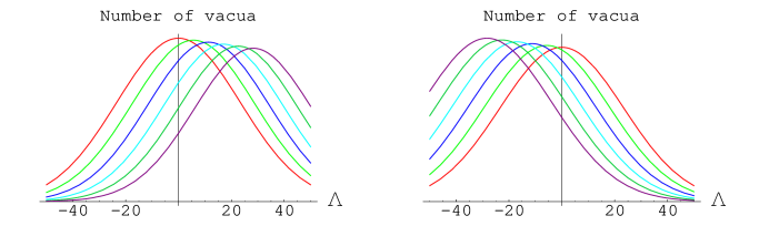
Figure 2: On the left we plot six normal distributions with mean $(i-1)566c$ and standard deviation $\sigma^{(total)}_{n,m}$ (see Eq. (33)) with $n=20$ and $m=\alpha n-i+1$, and here $1<i<6$. On the right we plot six normal distributions with mean $(1-i)566c$ and standard deviation $\sigma^{(total)}_{n,m}$ with $n=20$ and $m=\alpha n+i-1$, and again $1<i<6$. We take $c=10^{-2}$. The heights of these distributions are schematic - as we take more downward steps from a starting point, the number distribution grows, as indicated by the increasing height of the distributions from right to left in each plot.

We will classify all vacua in $0<\Lambda<c$ by two parameters: $n$ and $m$, where $n$ is the minimum number of up jumps required to reach a given vacuum from the dominant vacuum and $m$ is the number of down jumps. We will call $nm$ the level of the vacuum. Thus a vacuum of level $nm$ differs from the dominant vacuum in $n+m$ coordinates, $n$ of which are $+$ where the dominant vacuum had $-$, and another $m$ vice versa.

The total number of vacua of level $nm$ is thus

$$N_{nm}=N^{(up)}_{n}\times N^{(down)}_{m}$$ (36)

where

$$N^{(up)}_{n}=\left(\begin{array}[]{c}M\\ n\\ \end{array}\right)=\frac{M!}{n!(M-n)!}$$ (37)

and

$$N^{(down)}_{m}=\left(\begin{array}[]{c}P\\ m\\ \end{array}\right)=\frac{P!}{m!(P-m)!}$$ (38)

We approximate these to be smeared over a range $\sigma_{nm}$, where $\sigma_{nm}\equiv\sigma^{(total)}_{n,m}$, so their density is

$$\rho_{nm}=N_{nm}/\sigma_{nm}\equiv 1/\Delta_{nm}\,.$$ (39)

The likelihood that there is no vacuum in a range of size $x$ is $\exp(-\rho_{nm}x)$, thus the median $\Lambda$ of the lowest-$\Lambda$ vacuum is

$$\Lambda_{nm}=(\ln 2)/\rho_{nm}=\sigma_{nm}(\ln 2)/N_{nm}$$ (40)

We will assume the lowest-$\Lambda$ vacuum is at this median position. Above the lowest-$\Lambda$ vacuum of level $nm$, there are $N_{nm}-1$ more with higher $\Lambda$, with the typical interval in $\Lambda$ being $\Delta_{nm}$. For a typical realization it is sufficient to take these vacua as evenly spaced, so that they are at

$$\Lambda_{nm,\ell}=\Lambda_{nm}+(\ell-1)\Delta_{nm}$$ (41)

where $1\leq\ell\leq N_{nm}$.

This model is qualitatively different from the single step model studied in OSP . In the single step model, every vacuum in the range $(0,c)$ that was reached via $n$ up and necessarily $n$ down jumps (the so-called level $n$ vacua) would have the same number density $\rho_{n}$ (and also the same prior probability $P_{n}$). In fact, there is only one way to achieve a density of $\rho_{n}$ and that is to go up and down $n$ jumps. The next level would have $\rho_{n+1}\approx 500\rho_{n}$.

On the other hand, in the multi-step model, there are multiple classes of trajectories which can result in approximately the same densities $\rho_{nm}$. For example for $n=20$ and $m=\alpha n+1\sim 2.4n+1$, $\rho_{nm}\sim 7.3\times 10^{119}$ (and $\Lambda_{nm}\sim 9.5\times 10^{-121}$) while for $n=21$ and $m=\alpha n-2$ we find $\rho_{nm}\sim 2.4\times 10^{120}$ (and $\Lambda_{nm}\sim 2.8\times 10^{-121}$). In Table 1 we display where we expect the first vacuum $\Lambda_{nm}$ to lie for a range of values of $n$ and $m$. In Fig. 3 we depict where we expect some of these $\Lambda_{nm}$ vacua to lie, along with second and several subsequent vacua for the specific level according to Eq. (41).

m	n=19	n=20	n=21	n=22
$\alpha n+5$	$\mathbf{1.6\times 10^{-121}}$	$5.0\times 10^{-126}$	$1.9\times 10^{-130}$	$8.3\times 10^{-135}$
$\alpha n+4$	$\mathbf{3.4\times 10^{-120}}$	$1.0\times 10^{-124}$	$3.7\times 10^{-129}$	$1.5\times 10^{-133}$
$\alpha n+3$	$7.3\times 10^{-119}$	$2.1\times 10^{-123}$	$7.2\times 10^{-128}$	$2.9\times 10^{-132}$
$\alpha n+2$	$1.6\times 10^{-117}$	$\mathbf{4.4\times 10^{-122}}$	$1.4\times 10^{-126}$	$5.5\times 10^{-131}$
$\alpha n+1$	$3.6\times 10^{-116}$	$\mathbf{9.5\times 10^{-121}}$	$2.9\times 10^{-125}$	$1.1\times 10^{-129}$
$\alpha n$	$8.4\times 10^{-115}$	$2.1\times 10^{-119}$	$6.1\times 10^{-124}$	$2.1\times 10^{-128}$
$\alpha n-1$	$2.0\times 10^{-113}$	$4.7\times 10^{-118}$	$\mathbf{1.3\times 10^{-122}}$	$4.3\times 10^{-127}$
$\alpha n-2$	$4.8\times 10^{-112}$	$1.1\times 10^{-116}$	$\mathbf{2.8\times 10^{-121}}$	$9.0\times 10^{-126}$
$\alpha n-3$	$1.2\times 10^{-110}$	$2.5\times 10^{-115}$	$6.3\times 10^{-120}$	$1.9\times 10^{-124}$
$\alpha n-4$	$3.0\times 10^{-109}$	$6.0\times 10^{-114}$	$1.4\times 10^{-118}$	$\mathbf{4.1\times 10^{-123}}$
$\alpha n-5$	$7.8\times 10^{-108}$	$1.5\times 10^{-112}$	$3.3\times 10^{-117}$	$\mathbf{9.0\times 10^{-122}}$

Table 1: $\Lambda_{nm}$ for various values of $n$ and $m$ with $c=0.01$. We have highlighted some values to draw attention to the fact that paths reached via different levels can have almost the same $\Lambda_{mn}$ to within a factor of roughly 3 (and similarly for $\rho_{nm}$ and $\Delta_{nm}$): In particular when $(n,m)=(19,2.4n+4)$, $\Lambda_{nm}\sim 3.4\times 10^{-120}$. Then when $(n,m)=(20,\alpha n+1)$ $\Lambda_{nm}\sim 9.5\times 10^{-121}$ and for $(n,m)=(21,\alpha n-2)$, $\Lambda_{nm}\sim 2.8\times 10^{-121}$. Also for $(n,m)=(22,\alpha n-5)$, $\Lambda_{nm}\sim 9\times 10^{-122}$. As we went “diagonally” down, $\Lambda_{nm}$ decreased by a factor of $\sim 3$. The same pattern can be seen for the “diagonal” immediately above the one just discussed, starting with $(n,m)=(19,\alpha n+5)$ and $\Lambda_{nm}\sim 1.6\times 10^{-121}$.

Figure 3: Each line represents where we expect to find vacua. The highest line is at $\Lambda_{nm}\sim 3.4\times 10^{-120}$ with $n=19,m=\alpha n+4$. The next set of highest lines start at $\Lambda_{nm}\sim 9.5\times 10^{-121}$

and then are spaced by the corresponding $\Delta_{nm}$ with $n=20,m=\alpha n+1$. Also shown are two subsets of vacua reached via $n=21,m=\alpha n-2$ and $n=19,m=\alpha n+5$. Finally, the last and most dense set shown is for the first few vacua reached via $n=22,m=\alpha n-5$. The height of the lines has no meaning here. We simply want to show how different level $nm$ paths result in sets of vacua with similar densities. We have set $c=0.01$ here.

In principle, vacua reached via these different classes will have different probabilities. Also, there can even be a spread of probabilities amongst level $nm$ vacua, depending on the paths details. This spread is minimized for large jump sizes.

III Probabilities

We now use the formalism of Refs. GSPVW ; SPV outlined in Appendix C to calculate the relative abundances of different vacua in our toy model.

The relative abundance of each vacuum $\beta$ is given by a sum over all chains that connect it to the dominant vacuum, Eq. (100). The minimum number of transitions in such a chain is roughly $n+m$. Longer chains can be formed by jumping one way and then later the opposite way in the same direction. These chains will have extra suppression factors because of the extra jumps, but it remains a possibility that judiciously chosen “extra” jumps might enhance the probabilities enough to over compensate for these extra suppression factors. We will take the possibility of “extra” jumps into account when we calculate our numerical results. For now we shall we forget about them and include only minimum-length chains. Furthermore, the paths that maximize the bubble abundances are those that entail first making all the up jumps and then following with a sequence of down jumps. The reason is that the up-jump suppression factor, Eq. (99), is least when the starting $\Lambda$ for the jump is highest. Thus it is best not to jump down until all necessary up-jumps have been made.

Also, it can be shown that the path that contributes the most to the bubble abundance factor of a specific vacuum entails taking up-jumps in order of decreasing jump size while the down-jumps should be taken in increasing step sizes. This is because, jumps taken at lower $\Lambda^{\prime}s$ are more suppressed than those taken at higher $\Lambda^{\prime}s$, so the best strategy is to get to high-$\Lambda^{\prime}s$ as soon as possible.

We can reorganize Eq. (100),

$$p_{\beta}=\sum\frac{\kappa_{\beta a}}{D_{a}-D_{*}}\frac{\kappa_{ab}}{D_{b}-D_{*}}\cdots\frac{\kappa_{rs}}{D_{s}-D_{*}}\kappa_{st}\frac{\kappa_{tu}}{D_{t}-D_{*}}\cdots\frac{\kappa_{z*}}{D_{z}-D_{*}}$$ (42)

The transition rates to the right of the factor $\kappa_{st}$ in Eq. (100) are upward rates, and those to the left are downward rates. $\kappa_{st}$ represents the first downward jump after having made $n$ upward jumps from the dominant vacuum.

We will approximate $D_{*}\ll D_{j}$, since the transition rates are suppressed for low $\Lambda$ vacua. Now consider the denominator $D_{j}$.

$$D_{j}\propto\exp\left[\frac{-24\pi^{2}}{\Lambda_{j}}\tilde{r}_{jmin}\right]+\cdots+\exp\left[\frac{-24\pi^{2}}{\Lambda_{j}}\tilde{r}_{jmax}\right]$$ (43)

where $\tilde{r}_{jmin}$ is calculated from Eq.s (21) and (19) with $\Delta\Lambda_{a}$ in the smallest possible $\Delta\Lambda$ direction . We expect the smallest possible direction $\Delta\Lambda\sim 1c$.

Similarly $\tilde{r}_{jmax}$ is calculated with $\Delta\Lambda_{a}$ in the largest possible $\Delta\Lambda$ direction. All other terms in between have the same form with the $\tilde{r}_{j}$ factors taking on all relevant values as $\Delta\Lambda_{a}$ increases from the smallest to largest relevant values.

Using Eq. (99), the product of all up-jump suppression factors is

$$S=\left(\frac{\Lambda_{max}}{\Lambda_{*}}\right)^{2}\exp\left[-24\pi^{2}\left(\frac{1}{\Lambda_{*}}-\frac{1}{\Lambda_{max}}\right)\right]$$ (44)

where $\Lambda_{max}$ is the maximum $\Lambda$ reached for a given path.

The first term in the exponent above and the factor $\Lambda_{*}^{-2}$ will contribute to every vacuum reached via some path from the dominant vacuum and will thus disappear when we take ratios of probabilities. We define

$$\tilde{S}\equiv\exp\left[24\pi^{2}\left(\frac{1}{\Lambda_{max}}\right)\right]$$ (45)

and call it an up-jump “enhancement factor”.

Consider the last term in Eq. (42) which results from the first upward jump

$$\frac{\kappa_{z*}}{D_{z}-D_{*}}=\frac{\kappa_{*z}}{D_{z}-D_{*}}\left(\frac{\Lambda_{z}}{\Lambda_{*}}\right)^{2}\exp\left[-24\pi^{2}\left(\frac{1}{\Lambda_{*}}-\frac{1}{\Lambda_{z}}\right)\right]\approx\frac{\kappa_{*z}}{D_{z}}\left(\frac{\Lambda_{z}}{\Lambda_{*}}\right)^{2}\exp\left[-24\pi^{2}\left(\frac{1}{\Lambda_{*}}-\frac{1}{\Lambda_{z}}\right)\right]$$ (46)

Similarly, the product of $\kappa/D^{\prime}s$ for all the upward jumps can be written in terms of downward transition rates and an overall suppression factor as

$$\frac{\kappa_{tu}}{D_{t}-D_{*}}\cdots\frac{\kappa_{z*}}{D_{z}-D_{*}}\approx\frac{\kappa_{ut}}{D_{t}}\cdots\frac{\kappa_{*z}}{D_{z}}\left(\frac{\Lambda_{max}}{\Lambda_{*}}\right)^{2}\exp\left[-24\pi^{2}\left(\frac{1}{\Lambda_{*}}-\frac{1}{\Lambda_{max}}\right)\right].$$ (47)

Now we see that we can call $\kappa_{ij}/D_{j}$ a branching ratio, since it is the fraction of one possible downward transition rate from vacuum $\Lambda_{j}$ divided by the sum of all the possible downward transition rates from the same vacuum.

The down-jumps are similar, except that the first jump down from $\Lambda_{max}$ doesn’t have a factor of $D_{t}$ in the denominator (see Eq. (42)), giving

$$\frac{\kappa_{\beta a}}{D_{a}-D_{*}}\cdots\frac{\kappa_{rs}}{D_{s}-D_{*}}\kappa_{st}\approx\frac{\kappa_{\beta a}}{D_{a}}\frac{\kappa_{ab}}{D_{b}}\cdots\frac{\kappa_{rs}}{D_{s}}\kappa_{st}$$ (48)

III.1 The prior probability of a vacuum of level $nm$

The product of branching ratio’s for an upward path of $n$ jumps is

$$\prod_{\tilde{n}=1}^{n}\left(\frac{\kappa_{ij}}{D_{j}}\right)^{up}_{\tilde{n}} = \prod_{\tilde{n}=1}^{n}\left[\frac{\exp\left[\frac{-24\pi^{2}}{\Lambda_{j}}\tilde{r}_{j}(\Delta\Lambda_{\tilde{n}})\right]}{\left(\sum_{\ell=1}^{P}\exp\left[\frac{-24\pi^{2}}{\Lambda_{j}}\left[\tilde{r}_{j}(\Delta\Lambda_{\ell})\right]\right]+\sum_{q=1}^{\tilde{n}}\exp\left[\frac{-24\pi^{2}}{\Lambda_{j}}\left[\tilde{r}_{j}(\Delta\Lambda_{q})\right]\right]\right)}\right]$$ (49)

$$= \prod_{\tilde{n}=1}^{n}\left[\sum_{\ell=1}^{P}\exp\left[\frac{-24\pi^{2}}{\Lambda_{j}}\left[\tilde{r}_{j}(\Delta\Lambda_{\ell})-\tilde{r}_{j}(\Delta\Lambda_{\tilde{n}})\right]\right]+\sum_{q=1}^{\tilde{n}}\exp\left[\frac{-24\pi^{2}}{\Lambda_{j}}\left[\tilde{r}_{j}(\Delta\Lambda_{q})-\tilde{r}_{j}(\Delta\Lambda_{\tilde{n}})\right]\right]\right]^{-1}$$

where $P$ is the number of plus coordinates in the dominant vacuum configuration, and we define $\Delta\Lambda_{\tilde{n}}$ to be the change in $\Lambda$ for the $\tilde{n}^{\prime}th$ upward jump. Also, we have introduced the notation $\tilde{r}_{j}(\Delta\Lambda_{a})\equiv\tilde{r}(x,y)$ with $y=\frac{2\Lambda_{j}}{\Delta\Lambda_{a}}-1$ and $x=3/4$ (see Eq’s. (19,21)).

The second sum takes into account that for each upward jump, a coordinate that was $-$ becomes a $+$ coordinate, and therefore transitions downward in these directions must be included in $D_{j}$ when calculating the branching ratio.

Similarly, the product of branching ratio’s for a downward path with $m$ jumps is

$$\prod_{\tilde{m}=2}^{m}\left(\frac{\kappa_{ij}}{D_{j}}\right)^{down}_{\tilde{m}} = \prod_{\tilde{m}=2}^{m}\left[\sum_{\ell=1}^{P}\exp\left[\frac{-24\pi^{2}}{\Lambda_{j}}\left[\tilde{r}_{j}(\Delta\Lambda_{\ell})-\tilde{r}_{j}(\Delta\Lambda_{\tilde{m}})\right]\right]\right.$$ (50)

$$- \left.\sum_{m^{\prime}=1}^{\tilde{m}-1}\exp\left[\frac{-24\pi^{2}}{\Lambda_{j}}\left[\tilde{r}_{j}(\Delta\Lambda_{m^{\prime}})-\tilde{r}_{j}(\Delta\Lambda_{\tilde{m}})\right]\right]\right.$$

$$+ \left.\sum_{q=1}^{n}\exp\left[\frac{-24\pi^{2}}{\Lambda_{j}}\left[\tilde{r}_{j}(\Delta\Lambda_{q})-\tilde{r}_{j}(\Delta\Lambda_{\tilde{m}})\right]\right]\right]^{-1}$$

Since the first downward transition does not have a $D_{j}$ in the denominator (see Eq. (48)), our product of branching ratios starts with the second downward jump, thus $\tilde{m}$ starts at $2$ instead of $1$.

The first sum includes the contribution to $D_{j}$ from all the original $P$ $+$ coordinates in $\Lambda_{*}$. However, for each jump down on the return path, the next $\Lambda_{j}$ will have one less $+$ coordinate and thus the transition rate down in this “lost” direction, must not be included in $D_{j}$. Thus we subtract the second sum from the first to account for directions which were originally $+$’s but in which we can no longer jump down.

The third sum takes into account that the downward path jumps take place after $n$ upward jumps have changed $n$ coordinates from $-$ to $+$, and therefore transitions downward in these $n$ directions must be included in $D_{j}$ when calculating the branching ratio.

Thus the contribution of a path to the prior probability of a vacuum of level $nm$ is

$$P_{nm}\propto\prod_{\tilde{n}=1}^{n}\left(\frac{\kappa}{D}\right)^{up}\prod_{\tilde{m}=2}^{m}\left(\frac{\kappa}{D}\right)^{down}\kappa_{st}\left(\frac{\Lambda_{max}}{\Lambda_{*}}\right)^{2}\exp\left[-24\pi^{2}\left(\frac{1}{\Lambda_{*}}-\frac{1}{\Lambda_{max}}\right)\right]$$ (51)

with $\prod_{\tilde{n}=1}^{n}\left(\frac{\kappa}{D}\right)^{up}$ and $\prod_{\tilde{m}=2}^{m}\left(\frac{\kappa}{D}\right)^{down}$ as given by Eq’s. (49) and (50), and $\kappa_{st}$ is the first downward jump after having reached $\Lambda_{max}$ and is given by

$$\kappa_{st}\approx\exp\left[\frac{-24\pi^{2}}{\Lambda_{max}}\tilde{r}_{\Lambda_{max}}(\Delta\Lambda_{\tilde{m}=1})\right]$$ (52)

Clearly Eq. (51) is very complicated. There are $N_{nm}$ different vacua belonging to level $nm$ and each one has in principle a unique prior probability which depends on the details of the transitions made, and not just on the number of up and down jumps (as in the single step model). We need to stress the fact that for the MS model we have a distribution of prior probabilities for level $nm$ vacua, in contrast to the unique prior probability $P_{n}$ for level $n$ vacua in the single-step model. We cannot explicitly calculate all the possible probabilities for level $nm$ vacua, so we will consider two limiting cases of interest to us.

It seems reasonable that if $c$ is “large enough”, then individual transition rates are high and do not differ very much. Thus we expect that the spread in probabilities for level $nm$ vacua will be small. If the spread is small enough we can say that level $nm$ vacua have the same prior probability of $P_{nm}$. Also different orderings to reach the same vacuum should become roughly equally weighted.

On the other hand, if $c$ is “very small”, then the suppressed transition rates will differ markedly depending on path details and there will be a large spread in the prior probabilities of the different vacua within level $nm$.

In the next subsection we will try to quantify these heuristic expectations for the large $c$ regime.

The reader may find it useful at this point to turn to Appendix A where we study a simpler “averaged” version of our multi-step model analytically.

III.2 Large c approximation to the prior probability

For $c\sim 10^{-2}$ all the branching ratios in Eq’s. (49) and (50) reduce to 1/{number of possible directions in which downward transitions can be made} (see Fig.’s 4 and 5) and the prior becomes

$$P_{nm}\propto n!m!\prod_{\tilde{n}=1}^{n}\left(P+\tilde{n}\right)^{-1}\prod_{\tilde{m}=2}^{m}\left(P-(\tilde{m}-1)+\tilde{n}\right)^{-1}\Lambda_{max}^{2}\exp\left[\frac{24\pi^{2}}{\Lambda_{max}}\left(1-\tilde{r}_{\Lambda_{max}}(\Delta\Lambda_{\tilde{m}=1})\right)\right]$$ (53)

where we have dropped both factors in Eq. (51) which include $\Lambda_{*}$ since they will cancel when we take ratios of probabilities. Also, we have included the factor of $n!m!$ to account for the different order in which the transitions can be made to get to each level $nm$ vacuum. Strictly speaking some paths will be more heavily weighted than others and we should replace the factor $n!m!$ by some function $f(n,m)$. We assume here that $f(n,m)=\beta n!m!$ where we take $\beta$ to be a constant fraction for any specific value of $c$. Thus $\beta$ will drop out when we evaluate ratios of probabilities for different values of $nm$.

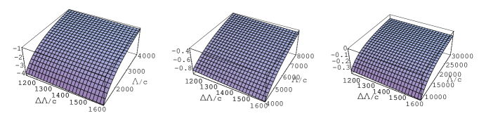
Figure 4: The purpose of these plots is to help us estimate the branching ratios contributing to the upward path for “large” $c=10^{-2}$. We show three surface plots spanning the possible $-B_{j}=\ln{\kappa_{ij}}$ with the following ranges for $\Lambda$: the first plot has $1133<\Lambda/c<4000$, the second has $4000<\Lambda/c<8000$ and the third has $8000<\Lambda/c<30000$. All three surfaces have $1133<\Delta\Lambda/c<1600$. Notice that along a contour of constant $\Lambda$, there is very little dependence on $\Delta\Lambda$. This shows that $\kappa/D\sim$ 1/{number of possible directions in which downward transitions can be made}.

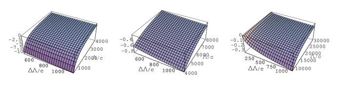
Figure 5: The purpose of these plots is to help us estimate the branching ratios contributing to the downward path for “large” $c=10^{-2}$. We show three surface plots spanning the possible $-B_{j}=\ln{\kappa_{ij}}$ with the following ranges for $\Lambda/c$ and $\Delta\Lambda/c$ : the first plot has $450<\Lambda/c<4000$ and $450<\Delta\Lambda/c<1132$, the second has $4000<\Lambda/c<8000$ and $450<\Delta\Lambda/c<1132$, while the third has $8000<\Lambda/c<30000$ and $1<\Delta\Lambda/c<1132$. Again we see that along a contour of constant $\Lambda$, the dependence on $\Delta\Lambda$ is weak.

Noting that

$$\prod_{\tilde{n}=1}^{n}\left(P+\tilde{n}\right)^{-1}=\frac{P!}{(P+n)!}$$ (54)

and

$$\prod_{\tilde{m}=2}^{m}\left(P-(\tilde{m}-1)+n\right)^{-1}=\frac{(P+n)(P+n-m)!}{(P+n)!}$$ (55)

the prior can be written as

$$P_{nm}\propto n!m!\frac{P!(P+n-m)!(P+n)}{\left((P+n)!\right)^{2}}\Lambda_{max}^{2}\exp\left[\frac{24\pi^{2}}{\Lambda_{max}}\left(1-\tilde{r}_{\Lambda_{max}}(\Delta\Lambda_{\tilde{m}=1})\right)\right]$$ (56)

III.3 Small $c$ regime and the prior probability

Let’s look at Fig’s. 4 and 5 again. If we were to re-plot these surfaces for smaller $c$, the only thing that would change would be the scale of the height. Since the tunneling exponent $B_{j}\propto 1/c$, smaller values of $c$ result in larger $B_{j}$ and thus more suppression. This indicates that as $c$ get’s smaller there is more of an absolute difference in the amount of suppression for jumps occuring in different directions from the same value of $\Lambda$. The net result is that different paths will have different prior probabilities even when comparing paths that have the same level $nm$ (this spread in probabilities for a given level was not present in the single-step and averaged multi-step models). Thus we cannot come up with a closed form simplified analytic expression for the prior probability in the small $c$ case. But we will show numerically that when $c\sim 10^{-3}$ vacua of the same level, reached via different paths, start to have prior probabilities which differ by several e-foldings. This allows for the possibility of a staggered distribution.

III.4 Numerical Interlude

Using numerics we will reinforce our claim that level $nm$ vacua have almost identical probabilities even if reached via different subclasses of trajectories for $c\sim 10^{-2}$. We will also reinforce our claim that already for $c\sim 10^{-3}$ path dependent differences cause a spread in probabilities amongst same level $nm$ vacua. We will consider the vacua reached via $n$ up jumps and $m=\alpha n$ down jumps with $n=19,20$ and $21$. We define three subclasses of trajectories as follows:

1. The “evenly spread out” trajectory: Let’s consider the $n$ up jumps first. There are $M=468$ $-$’ve directions to choose from to make our $n$ jumps. Thus we choose a trajectory such that within each interval of consecutive $M/n$ coordinates there will be one jump. We assume that each jump occurs at the mid-point of the interval. We calculate the probabilities by ordering the up jumps from largest to smallest. We do the same for the down jumps, only now we order jumps from smallest to largest and the size of the interval from which we pick our coordinates for each jump is given by $P/m$, where $P$ is the number of original plus coordinates in the dominant vacuum.

2. The “extreme” trajectory: Here we jump up in the largest $n/2$ possible directions, and then in the smallest $n/2$ directions out of the original $M$ coordinates. All the up jumps are ordered in decreasing step size. For the downward path we order jumps from smallest to largest starting with the $m/2$ smallest $+$ coordinates, and then ending with the $m/2$ largest $+$ directions.

3. The “clumped around the average value” trajectory: Again consider the upward path. We calculate the average value of $\Delta\Lambda$ for the $M$ directions we could go up in. We then consider the $n/2$ coordinates above to the $n/2$ coordinates below this average, and assume that our jumps are made from largest to smallest out of this consecutive range of integers. For the downward path we calculate the average $\Delta\Lambda$ for the original $P$ directions we could go down in. We then consider the $m/2$ coordinates above to the $m/2$ coordinates below this average, and assume that our jumps were made from smallest to largest out of this consecutive range of integers.

For each of these trajectories we numerically calculated the prior probability according to Eq. (51) for $c=10^{-2}$ and $c=10^{-3}$ for several values of $n$. The results are displayed in Tables 2 and 3 where we give the $-\ln P_{nm}$ for each case. Thus we see that indeed level $nm$ vacua have almost identical probabilities even if reached via different subclasses of trajectories for $c\sim 10^{-2}$, whilst for $c\sim 10^{-3}$ there is already a spread in the prior probabilities amongst level $nm$ vacua.

subclass	n=19	n=20	n=21
spread	454.63	475.73	496.84
extreme	453.67	474.74	495.81
clumped	452.57	473.68	494.78

Table 2: For $c=10^{-2}$ we find the round trip prior probability and display $-\ln{P_{nm}}$ for the three subclasses of trajectories discussed in the text. Results are shown for various values of $n$ and $m=\alpha n$. We see that, for a given $nm$, there is essentially no difference between the different trajectories. But the prior is a factor of $\sim 10^{9}$ times greater for $n=19$ than for $n=20$, and similarly for $n=20$ vs $n=21$. This is easily understood as follows. The $n+1$ trajectory has approximately 3 extra jumps over the $n$ trajectory (one for the extra up direction and roughly 2 extra in the down direction). Each one of these extra jumps contributes a factor of $\kappa/D\sim O(10^{-3})$ because there are roughly $1000$ directions to jump down in.

subclass	n=19	n=20	n=21
spread	545	566.58	587
extreme	528.9	549.85	570
clumped	564.2	585.27	606

Table 3: For $c=10^{-3}$ we find the round trip prior probability and display $-\ln{P_{nm}}$ for the three subclasses of trajectories discussed in the text. Results are shown for various values of $n$ and $m=\alpha n$. We see a large spread in probabilities amongst same level $nm$ vacua which makes it impossible for us to use our procedure for comparing observed probabilities in the anthropic range as we did in the single-step model, the AMS model discussed in the appendix, and as we will do in the large c multi-step case in Section IV.

Let’s now take a look at Fig. 6 where we plot $-\ln(\kappa/D)$ for each jump in an up and down path with $(n,m)=(20,48)$ and $c=10^{-2}$. The jumps up were made in order of decreasing jump size and the reverse order for the descent back down. The first few jumps have the highest values for the “branching ratio” suppression (we distinguish between the suppression caused by the branching ratio factors and the overall up-jump suppression which depends on how high up in $\Lambda$ we have to jump before the downward descent) because they are taking place in lower-$\Lambda$ backgrounds than the later small jumps in the path . The small jumps all take place where $\Lambda$ is already relatively large, and their suppression effects are marginalized. However, we must point out that even if a jump occurs at a high enough $\Lambda$ such that transition rates are unsuppressed, the branching ratio for the jump is still a fraction, $\kappa/D\approx 10^{-3}$, so that a path with more steps always pays some penalty.

Figure 6: On the left we show $-\ln(\kappa/D)$ (ie the branching ratio exponential suppression factors) for the “spread” up path plotted vs the number of the jump. On the right we show $-\ln(\kappa/D)$ for the “spread” down path plotted vs the “reverse” of the number of jumps (for example $10$ means the tenth to last downward jump and so on). We can see that transitions occurring from lower-$\Lambda$ (those closer to the y-axis) are more suppressed. Note also that all these value are pretty similar, which is to be expected since we are in the large $c$ regime with $c=10^{-2}$. The first two up path points are at $\{7.49,7.30\}$ but are not depicted. Also, not shown are the four points at $\{7.44,7.27,7.19,7.14\}$ closest to the y-axis for the downward path.

Figure 7: Same as previous plots except now $c=10^{-3}$. Note that the suppression is larger. The first few points are not displayed. For the up path they are $\{26.71,13.91\}$. The highest few values for the down path have also been omitted from the display. They are $\{36.40,17.65,12.37,10.21,9.14,8.55,...\}$ for the last jump, second last jump and so on.

IV Distribution for the observed $\Lambda$ in the large $c$ regime

We should now be convinced that in the large $c$ regime vacua of level $nm$ have the same prior $P_{nm}$. We thus have all the parts necessary to calculate the probability of observing each value $\Lambda_{nm,\ell}$ in a typical realization of our toy model. These are given by

$$P_{\text{obs}}(\Lambda_{nm,\ell})\propto P_{nm}n_{\text{obs}}(\Lambda_{nm,\ell})$$ (57)

The chance that we live in a world of a given level $nm$ is then given by

$$P_{\text{obs}}(nm)\propto P_{nm}\sum_{\ell}n_{\text{obs}}(\Lambda_{nm,\ell})$$ (58)

We will consider two cases.

1. When $\Lambda_{nm}\ll\Lambda_{c}$, the sum can be approximated by an integral,

   $$\sum_{\ell}n_{\text{obs}}(\Lambda_{nm,\ell})\approx\frac{1}{\Delta_{nm}}\int_{0}^{\infty}d\Lambda n_{\text{obs}}(\Lambda)=\frac{3\sqrt{\pi}\Lambda_{c}}{4\Delta_{nm}}=\frac{3\sqrt{\pi}N_{nm}\Lambda_{c}}{4\sigma_{nm}}=\frac{3\sqrt{\pi}\Lambda_{c}\ln 2}{4\Lambda_{nm}}$$ (59)

   and we find

   $$P_{\text{obs}}(nm) \propto \frac{3\sqrt{\pi}\Lambda_{c}}{4\sigma_{nm}}\frac{M!P!}{(M-n)!(P-m)!}\frac{P!(P+n-m)!(P+n)}{\left((P+n)!\right)^{2}}\Lambda_{max}^{2}$$ (60)

   $$\times \exp\left[\frac{24\pi^{2}}{\Lambda_{max}}\left(1-\tilde{r}_{\Lambda_{max}}(\Delta\Lambda_{\tilde{m}=1})\right)\right]$$

   where we used Eqs. (36, 37, 38, 56). We have not included the terms involving $\Lambda_{*}$, which are the same for all $P_{\text{obs}}(nm)$. In Eq. (60), $P_{\text{obs}}(nm)$ is a decreasing function of $n$.

2. When $\Lambda_{nm}>\Lambda_{c}$, Eq. (58) will be dominated by the first term, and we find

   $$\sum_{\ell}n_{\text{obs}}(\Lambda_{nm,\ell})\approx e^{-(\Lambda_{nm}/\Lambda_{c})^{2/3}}$$ (61)

   and

   $$P_{\text{obs}}(nm)\propto\frac{n!m!P!(P+n-m)!(P+n)}{\left((P+n)!\right)^{2}}\Lambda_{max}^{2}\exp\left[\frac{24\pi^{2}}{\Lambda_{max}}\left(1-\tilde{r}_{\Lambda_{max}}(\Delta\Lambda_{\tilde{m}=1})\right)-\left(\frac{\Lambda_{nm}}{\Lambda_{c}}\right)^{2/3}\right]$$ (62)

   In Eq. (62), $P_{\text{obs}}(nm)$ increases with increasing $n$ while $n$ is small and the last term in the exponent is dominant, but it decreases when $n$ is larger and the other terms are dominant.

IV.1 Comparison of probabilities for level $n+1,\alpha(n+1)+\gamma$ and $n,\alpha n+3+\gamma$ paths

From Table 1 we see that we are comparing probabilities of vacua which lie adjacent to one another along a “bold diagonal” and thus have similar number densities. For example; for $n=19,\gamma=1$ we would compare probabilities of the two levels $(n,(\alpha n+3)+\gamma)=(19,\alpha 19+4)$ and $(n+1,\alpha(n+1)+\gamma)=(20,\alpha 20+1)$. We have introduced the bookkeeping integer $-5<\gamma<2$.

1. When $\Lambda_{n,\alpha n+3+\gamma}>\Lambda_{c}$ and $\Lambda_{n+1,\alpha(n+1)+\gamma}>\Lambda_{c}$, and using Eq.(62)

   $$\frac{P_{obs}(n+1,\alpha(n+1)+\gamma)}{P_{obs}(n,\alpha n+3+\gamma)} \approx \frac{n+1}{(P+n+1)(P+n)}\frac{(\alpha n+\alpha+\gamma)!}{(\alpha n+3+\gamma)!}\frac{(P+n+1-\alpha(n+1)-\gamma)!}{(P+n-\alpha n-3-\gamma)!}$$ (63)

   $$\times \left(\frac{n+1}{n}\right)^{2}\exp\left[\left(\frac{\Lambda_{n,\alpha n+3+\gamma}}{\Lambda_{c}}\right)^{2/3}-\left(\frac{\Lambda_{n+1,\alpha(n+1)+\gamma}}{\Lambda_{c}}\right)^{2/3}\right]$$

   where we have approximated $\left(\frac{\Lambda_{max}(n+1)}{\Lambda_{max}(n)}\right)^{2}\approx\left(\frac{n+1}{n}\right)^{2}$. For $n\sim 20$, $\Lambda_{n,\alpha n+3+\gamma}\sim 3\Lambda_{n+1,\alpha(n+1)+\gamma}$, and we find

   $$\frac{P_{obs}(n+1,\alpha(n+1)+\gamma)}{P_{obs}(n,\alpha n+3+\gamma)} \approx \frac{n+1}{(P+n+1)(P+n)}\frac{(\alpha n+\alpha+\gamma)!}{(\alpha n+3+\gamma)!}\frac{(P+n+1-\alpha(n+1)-\gamma)!}{(P+n-\alpha n-3-\gamma)!}$$ (64)

   $$\times \left(\frac{n+1}{n}\right)^{2}\exp\left[\left(\frac{\Lambda_{n+1,\alpha(n+1)+\gamma}}{\Lambda_{c}}\right)^{2/3}\right]$$

   $$\approx 0.1\exp\left[\left(\frac{\Lambda_{n+1,\alpha(n+1)+\gamma}}{\Lambda_{c}}\right)^{2/3}\right]$$

   thus $P_{obs}(n+1,\alpha(n+1)+\gamma)\gg P_{obs}(n,\alpha n+3+\gamma)$. Therefore, in this regime $P_{obs}$ grows with decreasing $\Lambda$.

2. When $\Lambda_{n+1,\alpha(n+1)+\gamma}<\Lambda_{c}$ and $\Lambda_{n,\alpha n+3+\gamma}<\Lambda_{c}$, we find using Eq. (60)

   $$\frac{P_{obs}(n+1,\alpha(n+1)+\gamma)}{P_{obs}(n,\alpha n+3+\gamma)} \approx \frac{n+1}{(P+n+1)(P+n)}\frac{(\alpha n+\alpha+\gamma)!}{(\alpha n+3+\gamma)!}$$ (65)

   $$\times \left(\frac{n+1}{n}\right)^{2}\frac{(P+n+1-\alpha(n+1)-\gamma)!}{(P+n-\alpha n-3-\gamma)!}\frac{\Lambda_{n,\alpha n+3+\gamma}}{\Lambda_{n+1,\alpha(n+1)+\gamma}}$$

   $$\approx 0.3$$

Thus we find that several values of $nm$ contribute nearly equally to the total probability. The first of these might be dominated by a single $\Lambda_{n,\alpha n+3+\gamma}$, but there will be other vacua with closer spaced $\Lambda$. These vacua have similar $n_{\text{obs}}$ and identical prior probability, so we could easily be in any of them.

Thus when $c$ is large, we recover approximately the original anthropic predictions with a smooth prior $P(\Lambda)$. There might be an effect due to the discrete nature of the vacua associated with the smallest $(n,\alpha n+3+\gamma)$, where $P_{\text{obs}}(n,\alpha n+3+\gamma)$ has its peak, but this effect is small because level $(n,\alpha n+3+\gamma)$ does not dominate the probability distribution. Instead the probability is divided across many different levels, while only level $n,\alpha n+3+\gamma$ has the above effect. In other words, we may be more likely to be in the first $(n,\alpha n+3+\gamma)$ vacuum, but a good fraction of the probability is still spread amongst many other vacua. Thus the distribution is effectively flat.

IV.2 Comparison of probabilities for level $nm$ and $n,(m+1)$ paths

From Table 1 we see that level $n,(m+1)$ lie one row above the level $nm$ vacua. These vacua have number densities $\rho_{nm}$ which differ by roughly a factor of $20$. We will now evaluate the ratio of probabilities for vacua with levels which differ via one extra jump down.

1. When $\Lambda_{nm}>\Lambda_{c}$ and $\Lambda_{n(m+1)}>\Lambda_{c}$, and using Eq. (62)

   $$\frac{P_{obs}(n(m+1))}{P_{obs}(nm)}=\frac{m+1}{P+n-m}\exp\left[\left(\frac{\Lambda_{nm}}{\Lambda_{c}}\right)^{2/3}-\left(\frac{\Lambda_{n(m+1)}}{\Lambda_{c}}\right)^{2/3}\right]$$ (66)

   For $n\sim 20,m\sim 50$, $\Lambda_{nm}\sim 20\Lambda_{n(m+1)}$, thus $P_{obs}(n(m+1))\gg P_{obs}(nm)$

2. When $\Lambda_{nm}>\Lambda_{c}$ and $\Lambda_{n(m+1)}<\Lambda_{c}$, using Eq.’s (60,62) we find

   $$\frac{P_{obs}(n(m+1))}{P_{obs}(nm)}=\frac{m+1}{P+n-m}\frac{3\sqrt{\pi}\Lambda_{c}\ln{2}}{4\Lambda_{n(m+1)}}\exp\left[\left(\frac{\Lambda_{nm}}{\Lambda_{c}}\right)^{2/3}\right]\approx\frac{1}{20}\exp\left[\left(\frac{\Lambda_{nm}}{\Lambda_{c}}\right)^{2/3}\right]$$ (67)

   and therefore $P_{obs}(n(m+1))\gtrsim P_{obs}(nm)$.

3. When $\Lambda_{n(m+1)}<\Lambda_{c}$ and $\Lambda_{nm}<\Lambda_{c}$, using Eq. (60), we find

   $$\frac{P_{obs}(n(m+1))}{P_{obs}(nm)}=\frac{m+1}{P+n-m}\frac{\Lambda_{nm}}{\Lambda_{n(m+1)}}\approx 1.$$ (68)

We can also have vacua reached via $m+2$, $m+3$, … jumps down and all these vacua contribute nearly equally to the total probability. We could live in any one of these. Thus since level $nm$ doesn’t dominate over level $n(m+1)$, $n(m+2)$,… we again see evidence for an effectively flat distribution.

V Discussion

A key ingredient in the anthropic prediction of the cosmological constant is the assumption of a flat prior distribution. However, the first attempt to calculate this distribution for the Bousso-Polchinski and Arkani-Hamed-Dimopolous-Kachru landscape models SPV ; SP revealed a staggered distribution, suggesting a conflict with anthropic predictions.

These calculations were constrained by computational limitations and revealed only the probabilities of a handful of the most probable vacua. In Ref. OSP we went beyond these first order perturbative results by studying a simple toy model which allowed analytic calculation with a large, realistic number of vacua, $N\sim 10^{500}$. We found an interesting fractal distribution for the prior $P(\Lambda)$. When including anthropic selection effects to determine $P_{obs}(\Lambda)$, we found that agreement with observation depends on the only free parameter of the model, the jump size $\tilde{c}$.

We showed that when $\tilde{c}\sim 1$, anthropic reasoning does indeed solve the cosmological constant problem. Even though the prior distribution has a rich fractal structure, the states of interest have similar vacua sufficiently closely spaced to approximate the flat distribution well enough to give the usual anthropic results.

On the other hand, if $\tilde{c}$ is small, of order $10^{-3}$, then the agreement with observation was found to break down. In this case the volume fraction of universes with large cosmological constant is so high that in the overall probability they are greatly preferred even though the selection factor disfavors them.

We emphasize that the primary cause of the massive spread in probabilities in SPV ; SP which has been referred to as staggering, comes from differences in total up-jump suppression factors. This effect was studied analytically in OSP . Jumping to a higher $\Lambda_{max}$ causes any of the descendant vacua to be suppressed relative to descendants of lower $\Lambda_{max}$ paths. Since $\Lambda_{max}$ depends on the free parameter $\tilde{c}$, so does the relative suppression, and thus we can always tune $\tilde{c}$ for smooth or staggered distributions.

In this paper we have studied a multi-step model with a range of jump sizes,$|\Delta\Lambda_{i}|=ci$ and $1\leq i\leq J$, parameterized by an overall free parameter $c$. (We also studied a simpler averaged version of the model, which allowed more progress analytically, especially for the small $c$ scenario.) In OSP we conjectured that, for such a model, landscapes with large jumps are more likely to give the standard anthropic results, while those with small jumps are likely to predict universes unlike ours. We argued that the transition rates between vacua all have terms proportional to $1/c$ in the exponent. Thus when $c$ is small, the transition rates and the probabilities of different vacua are very sensitive to the details of the transitions. When $c$ is large, all rates are larger and less variable. This conjecture seems to be borne out by our study of the multi-step and AMS models here.

The conclusion for the multi-jump model, that we can find cases where anthropic reasoning is both valid and invalid depending on some free parameter $c$ is analogous to the conclusion reached for the single-jump model OSP . However, there are interesting qualitative differences in the behavior of the prior distributions. Perhaps we could be so bold as to turn the anthropic argument around, and use these results to predict what a sensible value for $c$ should be?

We should say a few words about boundary conditions at the regular Planck regime, $\Lambda\sim\mathcal{O}(M_{p}^{4})$. In particular, it may be that for the underlying fundamental theory, which we assume gives rise to the effective potential we have used in our ADK model, fluxes decompactify at the Planck scale and the effective potential asymptotes off to zero. If the fluxes do indeed decompactify it would seem like this Planck boundary would act as a sink for probability. We have not included these effects in our calculation because all of our transitions have taken place within the Planck boundary since even for $c=10^{-2}$ and $n\sim 20$, $\Lambda_{max}<320M_{P}^{4}\sim 0.5G^{-2}.$

One more speculative thought. If you consider a multi-jump model with less of a difference between the ratio of the largest to smallest jump in the range (in the current model the ratio is 1600 which is pretty big ) this could lead to a smoothing of the prior distribution for a reasonably small value of $c$. If the ratio of maximum and minimum jump sizes were constrained to be say within an order of magnitude, it could turn out that we can define a unique prior for a given level $nm$ vacuum, in the small $c$ case too. In so doing we would then be able to show that the observed distribution smooths out by comparing $P_{obs}$ for levels $nm$ and $n,m+1$ as we did in the large $c$ case.

Appendix A The “averaged” multi-step model

The dominant vacuum of the multi-step model we have been considering has roughly the following structure:

$$\Lambda_{*}=c\{+.....+-...-\}$$ (69)

with $P=0.71J\approx 1132$ $+$’s and $M=0.29J\approx 468$ $-$’s. Jumps down from the plus coordinates range in size from $1c\leq\Delta\Lambda\leq 1132c$ and jumps up from the minus coordinates range in size from $1133c\leq\Delta\Lambda\leq 1600c$.

The average jump size of the plus and minus coordinates respectively are $\Delta\bar{\Lambda}_{P}\approx 566c$ and $\Delta\bar{\Lambda}_{M}\approx 1366c$. We will define an “averaged” multi-step model (AMS model) which has a dominant vacuum with $P$ plus coordinates all having the same jump size $\Delta\bar{\Lambda}_{P}$ and $M$ minus coordinates all having the same jump size $\Delta\bar{\Lambda}_{M}$.

One of the simplifying characteristics of the AMS model is that vacua reached via $n$ up jumps and $m$ down jumps from the dominant vacuum all have the same prior probability, $P_{n}$, which we will now calculate.

A.1 The prior probability of the AMS model

The product of branching ratio’s for an upward path of $n$ jumps is

$$\prod_{\tilde{n}=1}^{n}\frac{\kappa_{ij}}{D_{j}}=\prod_{\tilde{n}=1}^{n}\left[P\exp\left[\frac{-24\pi^{2}}{\Lambda_{j}}\left[\tilde{r}_{j}(\Delta\bar{\Lambda}_{P})-\tilde{r}_{j}(\Delta\bar{\Lambda}_{M})\right]\right]+\tilde{n}\right]^{-1}$$ (70)

where $\Lambda_{j}=\tilde{n}\Delta\bar{\Lambda}_{M}+\Lambda_{*}$.

The product of branching ratio’s for the downward path with $m$ jumps is

$$\prod_{\tilde{m}=2}^{m}\frac{\kappa_{ij}}{D_{j}}=\prod_{\tilde{m}=2}^{m}\left[\left(P-(\tilde{m}-1)\right)+n\exp\left[\frac{-24\pi^{2}}{\Lambda_{j}}\left[\tilde{r}_{j}(\Delta\bar{\Lambda}_{M})-\tilde{r}_{j}(\Delta\bar{\Lambda}_{P})\right]\right]\right]^{-1}$$ (71)

and in this expression $\Lambda_{j}=n\Delta\bar{\Lambda}_{M}+\Lambda_{*}-(\tilde{m}-1)\Delta\bar{\Lambda}_{P}=\Lambda_{max}-(\tilde{m}-1)\Delta\bar{\Lambda}_{P}$.

Thus the prior probability of a vacuum of level $n$ is

$$P_{n}\propto n!m!\prod_{\tilde{n}=1}^{n}\left(\frac{\kappa}{D}\right)^{up}\prod_{\tilde{m}=2}^{m}\left(\frac{\kappa}{D}\right)^{down}\kappa_{st}\left(\frac{\Lambda_{max}}{\Lambda_{*}}\right)^{2}\exp\left[-24\pi^{2}\left(\frac{1}{\Lambda_{*}}-\frac{1}{\Lambda_{max}}\right)\right]$$ (72)

with $\prod_{\tilde{n}=1}^{n}\left(\frac{\kappa}{D}\right)^{up}$ and $\prod_{\tilde{m}=2}^{m}\left(\frac{\kappa}{D}\right)^{down}$ as given by Eq’s. (70) and (71), and $\kappa_{st}$ is the first downward jump after having reached $\Lambda_{max}$ and is given by

$$\kappa_{st}\approx\exp\left[\frac{-24\pi^{2}}{\Lambda_{max}}\tilde{r}_{\Lambda_{max}}(\Delta\bar{\Lambda}_{P})\right]$$ (73)

Notice that we have included an extra factor of $n!m!$ to account for all the equally weighted paths that lead to the same vacuum because the up jumps and down jumps can be taken in any order.

A.2 Large c approximation to the prior probability of the AMS model

For $c\sim 10^{-2}$ all the exponential factors in Eq’s. (70) and (71) reduce to $1$ and the prior becomes

$$P_{n}\propto n!m!\prod_{\tilde{n}=1}^{n}\left(P+\tilde{n}\right)^{-1}\prod_{\tilde{m}=2}^{m}\left(P-(\tilde{m}-1)+n\right)^{-1}\Lambda_{max}^{2}\exp\left[\frac{24\pi^{2}}{\Lambda_{max}}\left(1-\tilde{r}_{\Lambda_{max}}(\Delta\bar{\Lambda}_{P})\right)\right]$$ (74)

where we have dropped the $\Lambda_{*}$ terms appearing in Eq. (72).

Noting that

$$\prod_{\tilde{n}=1}^{n}\left(P+\tilde{n}\right)^{-1}=\frac{P!}{(P+n)!}$$ (75)

and

$$\prod_{\tilde{m}=2}^{m}\left(P-(\tilde{m}-1)+n\right)^{-1}=\frac{(P+n)(P+n-m)!}{(P+n)!}$$ (76)

the prior can be written as

$$P_{n}\propto n!m!\frac{P!(P+n-m)!(P+n)}{\left((P+n)!\right)^{2}}\Lambda_{max}^{2}\exp\left[\frac{24\pi^{2}}{\Lambda_{max}}\left(1-\tilde{r}_{\Lambda_{max}}(\Delta\bar{\Lambda}_{P})\right)\right]$$ (77)

A.3 Small c approximation to the prior probability of the AMS model

For $c\sim 10^{-4}$ the first exponential factor in Eq. (70) becomes large and we can ignore the second term. In Eq. (71) the second term becomes very small and can be ignored so the prior becomes

$$P_{n} \propto n!m!\prod_{\tilde{n}=1}^{n}\left[P\exp\left[\frac{-24\pi^{2}}{\Lambda_{j}}\left[\tilde{r}_{j}(\Delta\bar{\Lambda}_{P})-\tilde{r}_{j}(\Delta\bar{\Lambda}_{M})\right]\right]\right]^{-1}\prod_{\tilde{m}=2}^{m}\left(P-(\tilde{m}-1)\right)^{-1}$$ (78)

$$\Lambda_{max}^{2}\exp\left[\frac{24\pi^{2}}{\Lambda_{max}}\left(1-\tilde{r}_{\Lambda_{max}}(\Delta\bar{\Lambda}_{P})\right)\right]$$

where $\Lambda_{j}=\tilde{n}\Delta\bar{\Lambda}_{M}+\Lambda_{*}$ above.

Noting that

$$\prod_{\tilde{m}=2}^{m}\left(P-(\tilde{m}-1)\right)^{-1}=\frac{P(P-m)!}{P!}$$ (79)

we finally have

$$P_{n}\propto n!m!\frac{P(P-m)!}{P^{n}P!}\prod_{\tilde{n}=1}^{n}\left[\exp\left[\frac{-24\pi^{2}}{\Lambda_{j}}\left[\tilde{r}_{j}(\Delta\bar{\Lambda}_{M})-\tilde{r}_{j}(\Delta\bar{\Lambda}_{P})\right]\right]\right]\Lambda_{max}^{2}\exp\left[\frac{24\pi^{2}}{\Lambda_{max}}\left(1-\tilde{r}_{\Lambda_{max}}(\Delta\bar{\Lambda}_{P})\right)\right]$$ (80)

Appendix B Distribution for the observed $\Lambda$ in the AMS model

We now have all the parts necessary to calculate the probability of observing each value $\Lambda_{n,\ell}$ in a typical realization of our toy AMS model. These are given by

$$P_{\text{obs}}(\Lambda_{n,\ell})\propto P_{n}n_{\text{obs}}(\Lambda_{n,\ell})$$ (81)

The chance that we live in a world of a given level $n$ is then given by

$$P_{\text{obs}}(n)\propto P_{n}\sum_{\ell}n_{\text{obs}}(\Lambda_{n,\ell})$$ (82)

We will consider two cases.

1. When $\Lambda_{n}\ll\Lambda_{c}$, the sum can be approximated by an integral,

   $$\sum_{\ell}n_{\text{obs}}(\Lambda_{n,\ell})\approx\frac{1}{\Delta_{n}}\int_{0}^{\infty}d\Lambda n_{\text{obs}}(\Lambda)=\frac{3\sqrt{\pi}\Lambda_{c}}{4\Delta_{n}}=\frac{3\sqrt{\pi}N_{n}\Lambda_{c}}{4c}=\frac{3\sqrt{\pi}\Lambda_{c}\ln 2}{4\Lambda_{n}}$$ (83)

   where we have used $\sigma_{nm}\equiv c$ and therefore $N_{n}/c=1/\Delta_{n}$. We dropped the extra subscript of $m$ for $N_{nm}$ and $\Delta_{nm}$ since in the AMS model, once we specify $n$, $m=\alpha n$ is specified too.

2. When $\Lambda_{n}>\Lambda_{c}$, Eq. (82) will be dominated by the first term, and we find

   $$\sum_{\ell}n_{\text{obs}}(\Lambda_{n,\ell})\approx e^{-(\Lambda_{n}/\Lambda_{c})^{2/3}}$$ (84)

B.1 Large c regime

1. For $\Lambda_{n}\ll\Lambda_{c}$, and including Eqs. (36, 37, 38, 77), we find

   $$P_{\text{obs}}(n)\propto\frac{3\sqrt{\pi}\Lambda_{c}}{4c}\frac{M!P!}{(M-n)!(P-m)!}\frac{P!(P+n-m)!(P+n)}{\left((P+n)!\right)^{2}}\Lambda_{max}^{2}\exp\left[\frac{24\pi^{2}}{\Lambda_{max}}\left(1-\tilde{r}_{\Lambda_{max}}(\Delta\bar{\Lambda}_{P})\right)\right]$$ (85)

   We have not included the terms involving $\Lambda_{*}$, which are the same for all $P_{\text{obs}}(n)$. In Eq. (85), $P_{\text{obs}}(n)$ is a decreasing function of $n$.

2. When $\Lambda_{n}>\Lambda_{c}$, using Eq. (77), we find

   $$P_{\text{obs}}(n)\propto\frac{n!m!P!(P+n-m)!(P+n)}{\left((P+n)!\right)^{2}}\Lambda_{max}^{2}\exp\left[\frac{24\pi^{2}}{\Lambda_{max}}\left(1-\tilde{r}_{\Lambda_{max}}(\Delta\bar{\Lambda}_{P})\right)-\left(\frac{\Lambda_{n}}{\Lambda_{c}}\right)^{2/3}\right]$$ (86)

   In Eq. (86), $P_{\text{obs}}(n)$ increases with increasing $n$ while $n$ is small and the last term in the exponent is dominant, but it decreases when $n$ is larger and the other terms are dominant.

The division between regimes occurs when $\Lambda_{n}\sim\Lambda_{c}$, i.e.,

$$c\ln 2/N_{n}\sim\Lambda_{c}\sim 6\times 10^{-120}$$ (87)

With $c\sim 10^{-2}$, we find $n\sim 19/20$. The dependence on $c$ is weak, with $c\sim 10^{-4}$ corresponding to $n\sim 19$. For $n$ in this range, changing $n$ by one unit changes $\Lambda_{n}$ by a factor of about $10^{4}$. Thus there is at most one $n$ with $\Lambda_{n}\sim\Lambda_{c}$.

Comparing Eq.’s (85) and Eq. (86) for the same $n$, we see that they differ by a factor of $\Lambda_{c}N_{n}/c\exp{(\Lambda_{n}/\Lambda_{c})^{2/3}}\sim 1$ if $\Lambda_{n}\sim\Lambda_{c}$, so there is no big jump due to switching regimes.

Now let us start with $n=1$ and increase $n$. Certainly with $n=1$, $\Lambda_{n}\gg\Lambda_{c}$ by a huge factor, we are in the regime of Eq. (86), and $P_{\text{obs}}$ is infinitesimal. As we increase $n$, $P_{\text{obs}}$ increases. Once $n$ is significantly above 1, we can approximate the increase from one step to the next as

$$\frac{P_{\text{obs}}(n+1)}{P_{\text{obs}}(n)} \approx \left(\frac{(n+1)(\alpha(n+1))!(P+n+1-\alpha(n+1))!}{(P+n+1)(\alpha n)!(P+n-\alpha n)!(P+n)}\right)$$ (88)

$$\times \left(\frac{n+1}{n}\right)^{2}\exp\left[-\frac{24\pi^{2}}{cn^{2}\Delta\bar{\Lambda}_{M}}(1-\tilde{r}(\Delta\bar{\Lambda}_{P}))+\left(\frac{\Lambda_{n}}{\Lambda_{c}}\right)^{2/3}\right]$$

where we have ignored $\left(\Lambda_{n+1}/\Lambda_{c}\right)^{2/3}$ as much less than $\left(\Lambda_{n}/\Lambda_{c}\right)^{2/3}$ and used

$$\left(\frac{\Lambda_{max}(n+1)}{\Lambda_{max}(n)}\right)^{2}=\left(\frac{n+1}{n}\right)^{2}$$ (89)

$\sim 1.1$ for parameters of interest. In the first term $\tilde{r}(\Delta\bar{\Lambda}_{P})<<1$ for $n\sim 19$, so we will ignore this contribution.

Also, since we are in the regime of large $c\approx 10^{-2}$, for $J=1600$, $n\sim 19$, the first term in the exponent is $<-1$. Thus, for sufficiently small $n$, the last term in the exponent dominates and $P_{\text{obs}}(n+1)/P_{\text{obs}}(n)\gg 1$. There is only an infinitesimal probability that we will be in a vacuum of level $n$, because there are others that are much more probable. As we increase $n$, $P_{\text{obs}}(n)$ will continue to increase.

By the time we reach the point where $\Lambda_{n}\sim\Lambda_{c}$ the exponential term becomes insignificant.

In that case, we switch to the regime of Eq. (85), where $P_{\text{obs}}$ decreases only slowly with increasing $n$. In this regime,

$$\frac{P_{\text{obs}}(n+1)}{P_{\text{obs}}(n)}\approx\frac{N_{n+1}}{N_{n}}\frac{P_{n+1}}{P_{n}}\left(\frac{n+1}{n}\right)^{2}$$ (90)

which is about $0.41$ for parameters of interest. Thus we find that several values of $n$ contribute nearly equally to the total probability. The first of these might be dominated by a single $\Lambda_{n}$, but the others will have a large number of closely spaced $\Lambda$. These vacua have similar $n_{\text{obs}}$ and identical prior probability, so we could easily be in any of them.

Thus when $c$ is large, we recover approximately the original anthropic predictions with a smooth prior $P(\Lambda)$. There might be an effect due to the discrete nature of the vacua associated with the smallest $n$, where $P_{\text{obs}}(n)$ has its peak, but this effect is small because level $n$ does not dominate the probability distribution. Instead the probability is divided across many different levels, while only level $n$ has the above effect.

B.2 Small c regime

1. For $\Lambda_{n}\ll\Lambda_{c}$, and including Eqs. (36, 37, 38, 80), we find

   $$P_{\text{obs}}(n) \propto \frac{3\sqrt{\pi}\Lambda_{c}}{4c}\frac{M!}{(M-n)!}\frac{P}{P^{n}}\Lambda_{max}^{2}\exp\left[\frac{24\pi^{2}}{\Lambda_{max}}\left(1-\tilde{r}_{\Lambda_{max}}(\Delta\bar{\Lambda}_{P})\right)\right]$$ (91)

   $$\times \prod_{\tilde{n}=1}^{n}\left[\exp\left[\frac{-24\pi^{2}}{\Lambda_{j}}\left[\tilde{r}_{j}(\Delta\bar{\Lambda}_{M})-\tilde{r}_{j}(\Delta\bar{\Lambda}_{P})\right]\right]\right]$$

   In Eq. (91), $P_{\text{obs}}(n)$ is a decreasing function of $n$.

2. When $\Lambda_{n}>\Lambda_{c}$, using Eq. (80), we find

   $$P_{\text{obs}}(n) \propto \frac{n!m!P(P-m)!}{P^{n}P!}\Lambda_{max}^{2}\exp\left[\frac{24\pi^{2}}{\Lambda_{max}}\left(1-\tilde{r}_{\Lambda_{max}}(\Delta\bar{\Lambda}_{P})\right)-\left(\frac{\Lambda_{n}}{\Lambda_{c}}\right)^{2/3}\right]$$ (92)

   $$\times \prod_{\tilde{n}=1}^{n}\left[\exp\left[\frac{-24\pi^{2}}{\Lambda_{j}}\left[\tilde{r}_{j}(\Delta\bar{\Lambda}_{M})-\tilde{r}_{j}(\Delta\bar{\Lambda}_{P})\right]\right]\right]$$

   In Eq. (92), $P_{\text{obs}}(n)$ increases with increasing $n$ while $n$ is small and the last term in the exponent is dominant, but it decreases when $n$ is larger and the other terms are dominant.

Now let us start with $n=1$ and increase $n$. Again, with $n=1$, $\Lambda_{n}\gg\Lambda_{c}$ by a huge factor, we are in the regime of Eq. (92), and $P_{\text{obs}}$ is infinitesimal. As we increase $n$, $P_{\text{obs}}$ increases. Once $n$ is significantly above 1, we can approximate the increase from one step to the next as

$$\frac{P_{\text{obs}}(n+1)}{P_{\text{obs}}(n)}\approx\frac{n+1}{P}\frac{(\alpha(n+1))!}{(\alpha n)!}\frac{(P-\alpha(n+1))!}{(P-\alpha n)!}\left(\frac{n+1}{n}\right)^{2}\exp\left[-\frac{24\pi^{2}}{n^{2}\Delta\bar{\Lambda}_{M}}+\left(\frac{\Lambda_{n}}{\Lambda_{c}}\right)^{2/3}\right]$$ (93)

where we have ignored $\left(\Lambda_{n+1}/\Lambda_{c}\right)^{2/3}$ as much less than $\left(\Lambda_{n}/\Lambda_{c}\right)^{2/3}$. (For $1<n<21$ the prefactor is $\mathcal{O}(10^{-2}/10^{-3})$).

For sufficiently small $n$, the last term in the exponent dominates and $P_{\text{obs}}(n+1)/P_{\text{obs}}(n)\gg 1$. There is only an infinitesimal probability that we will be in a vacuum of level $n$, because there are others that are much more probable. As we increase $n$, $P_{\text{obs}}(n)$ will continue to increase. What happens next depends on the magnitude of $c$.

Let’s suppose that

$$c<\left(\frac{\Lambda_{n+1}}{\Lambda_{n}}\right)^{2/3}\frac{24\pi^{2}}{n^{2}\left(\Delta\bar{\Lambda}_{M}/c\right)}$$ (94)

for relevant values of $n$.

Thus we can find a value of $n$ such that

$$1<\left(\frac{\Lambda_{n+1}}{\Lambda_{n}}\right)^{2/3}\frac{24\pi^{2}}{n^{2}\left(\Delta\bar{\Lambda}_{M}\right)}<\left(\frac{\Lambda_{n}}{\Lambda_{c}}\right)^{2/3}<\frac{24\pi^{2}}{n^{2}\left(\Delta\bar{\Lambda}_{M}\right)}$$ (95)

We will now show that for this $n$,

$$P_{\text{obs}}(n+1)\ll P_{\text{obs}}(n)\,,$$ (96)

so that we should find ourselves in a vacuum of at most level $n$.

It is not clear from Eq. (95) whether $\Lambda_{n+1}/\Lambda_{c}$ is more or less than 1, so we might need to use either Eq. (91) or Eq. (92) for $P_{\text{obs}}(n+1)$. We will prove the claim using Eq. (91). Since this gives a larger value than Eq. (92), if Eq. (96) holds using Eq. (91), it will certainly hold using Eq. (92). Thus we will take

$$\frac{P_{\text{obs}}(n+1)}{P_{\text{obs}}(n)}\approx\frac{3\sqrt{\pi}\Lambda_{c}\ln{2}}{4\Lambda_{n+1}}\frac{(n+1)}{P}\frac{(\alpha(n+1))!}{(\alpha n)!}\frac{(P-\alpha(n+1))!}{(P-\alpha n)!}\left(\frac{n+1}{n}\right)^{2}\exp\left[-\frac{24\pi^{2}}{n^{2}\Delta\bar{\Lambda}_{M}}+\left(\frac{\Lambda_{n}}{\Lambda_{c}}\right)^{2/3}\right]$$ (97)

Now from Eq. (94), we find that

$$\frac{24\pi^{2}}{n^{2}\Delta\bar{\Lambda}_{M}}>\left(\frac{\Lambda_{n}}{\Lambda_{n+1}}\right)^{2/3}\approx\left(\frac{N_{n+1}}{N_{n}}\right)^{2/3}\approx 10^{8/3}$$ (98)

Thus unless $(\Lambda_{n}/\Lambda_{c})^{2/3}$ is extremely close to the upper bound in Eq. (95), the exponential term in Eq. (97) will be infinitesimal, and Eq. (96) will follow. If we do have $(\Lambda_{n}/\Lambda_{c})^{2/3}\approx 24\pi^{2}/(n^{2}\Delta\bar{\Lambda}_{M})$, then $\Lambda_{n+1}/\Lambda_{c}\gtrsim 1$. Then the prefactors in Eq. (97) are at most about $10^{-2}$ for parameters of interest, and again Eq. (96) follows.

Thus we can say with great confidence that we live in a universe with level $n$ or lower. From Eq. (95), we see immediately that we should observe $\Lambda\geq\Lambda_{c}$, whereas in fact we observe $\Lambda_{0}\approx 0.1\Lambda_{c}$. If $c$ is significantly smaller than the limit in Eq. (94), then we will see a very “non-anthropic” universe.

Appendix C Bubble abundances

We review here the procedure for calculating the volume fraction of vacua of a given kind, using the “pocket-based measure” formalism of Refs. GSPVW ; SPV .

Transition rates depend on the details of the landscape. However, if $\Lambda_{i}<\Lambda_{j}$, the rate of the transition upward from $i$ to $j$ is suppressed relative to the inverse, downward transition, by a factor which does not depend on the details of the process EWeinberg ,

$$\kappa_{ji} = \kappa_{ij}\left(\frac{H_{j}}{H_{i}}\right)^{4}\exp\left[-24\pi^{2}\left(\frac{1}{\Lambda_{i}}-\frac{1}{\Lambda_{j}}\right)\right]$$ (99)

$$= \kappa_{ij}\left(\frac{\Lambda_{j}}{\Lambda_{i}}\right)^{2}\exp\left[-24\pi^{2}\left(\frac{1}{\Lambda_{i}}-\frac{1}{\Lambda_{j}}\right)\right]$$

Given the entire set of rates $\kappa_{ij}$, we can in principle compute the bubble abundance $p_{\alpha}$ for each vacuum $\alpha$, following the methods of Refs. GSPVW ; SPV . An exact calculation would require diagonalizing an $N\times N$ matrix. But as in Ref. SPV , we can make the approximation that all upward transition rates are tiny compared to all downward transition rates from a given vacuum.

Once we have identified the dominant vacuum, the probability for any vacuum $\alpha$ is given by (see the next section)

$$p_{\alpha}=\sum\frac{\kappa_{\alpha a}\kappa_{ab}\cdots\kappa_{z*}}{(D_{a}-D_{*})(D_{b}-D_{*})\cdots(D_{z}-D_{*})}$$ (100)

where the sum is taken over all chains of intermediate vacua $a,b,\ldots,z$ that connect the vacuum $\alpha$ to the dominant vacuum.

C.1 Bubble abundances by perturbation theory

As shown in Ref. GSPVW , the calculation of bubble abundances $p_{j}$ reduces to finding the smallest eigenvalue $q$ and the corresponding eigenvector $s$ for a huge $N\times N$ recycling transition matrix $\mathbf{R}$. Bubble abundances are given by

$$p_{j}\propto\sum_{\alpha}H_{\alpha}^{q}\kappa_{j\alpha}s_{\alpha}\approx\sum_{\alpha}\kappa_{j\alpha}s_{\alpha}.$$ (101)

where the summation is over all recyclable vacua which can directly tunnel to $j$. $H_{\alpha}$ is the Hubble expansion rate in vacuum $\alpha$ and we take $H_{\alpha}^{q}\approx 1$ because $q$ is an exponentially small number.

In a realistic model, we expect $N$ to be very large. In the numerical example of Ref. SPV $N\sim 10^{7}$, while for a realistic string theory landscape we expect $N\sim 10^{500}$  Susskind ; Douglas ; AshokDouglas ; DenefDouglas . Solving for the dominant eigenvector for such huge matrices is numerically impossible. However, in Ref. SPV ; SPthesis the eigenvalue problem was solved via perturbation theory, with the upward transition rates (see Eq. (99)) playing the role of small expansion parameters. Here we extend this procedure to all orders of perturbation theory.

We represent our transition matrix as a sum of an unperturbed matrix and a small correction,

$$\mathbf{R}=\mathbf{R^{(0)}}+\mathbf{R^{(1)}},$$ (102)

where $\mathbf{R^{(0)}}$ contains all the downward transition rates and $\mathbf{R^{(1)}}$ contains all the upward transition rates. We will solve for the zero’th order dominant eigensystem $\{q^{(0)},\mathbf{s^{(0)}}\}$ from $\mathbf{R^{(0)}}$ and then include contributions from $\mathbf{R^{(1)}}$ to all orders of perturbation theory.

If the vacua are arranged in the order of increasing $\Lambda$, so that

$$\Lambda_{1}\leq\Lambda_{2}\leq\ldots\leq\Lambda_{N},$$ (103)

then $\mathbf{R^{(0)}}$ is an upper triangular matrix. Its eigenvalues are simply equal to its diagonal elements,

$$R^{(0)}_{\alpha\alpha}=-\sum_{j<\alpha}\kappa_{j\alpha}\equiv-D_{\alpha}.$$ (104)

Hence, the magnitude of the smallest zeroth-order eigenvalue is

$$q^{(0)}=D_{{*}}\equiv{\rm min}\{D_{\alpha}\}.$$ (105)

Downward transitions from ${*}$ will bring us to the negative-$\Lambda$ territory of terminal vacua SPV . Terminal vacua do not belong in the matrix $\mathbf{R}$; hence, $R_{\beta{*}}=0$ for $\beta\neq{*}$, and we see that the zeroth order eigenvector has a single nonzero component,

$$s^{(0)}_{\alpha}=\delta_{\alpha{*}}.$$ (106)

Thus, in fact, we could have included only the diagonal elements of $\mathbf{R^{(0)}}$ and still obtained the correct $q^{(0)}$ and $\mathbf{s^{(0)}}$.

Now we would like to include the effect of the upward transition rates in the lower triangular matrix $\mathbf{R^{(0)}}$, to any given order of perturbation theory. To organize the calculation, we note that the eigenvalues of an upper triangular matrix are just the diagonal elements, and the eigenvectors are given exactly by the perturbation series, which terminates after $N$ terms. Thus we will take just the diagonal elements of $\mathbf{R^{(0)}}$ as our unperturbed matrix, and consider the rest of $\mathbf{R^{(0)}}$ and $\mathbf{R^{(1)}}$ as a perturbation. By summing all terms in the perturbation series for this perturbation that involve $n$ elements of $\mathbf{R^{(1)}}$, we find the perturbation term of order $n$ in the small upward jump rates.

The procedure is the same as that involved in finding an eigenstate of the Schrödinger equation in $n$th-order perturbation theory, working in a basis of wavefunctions which diagonalize the unperturbed equation. See for example Eq. (9.1.16) of Ref. MorseFeshbach . Including all orders of perturbation theory, we find the result

$$s_{a}=\sum_{b=1}^{N}\cdots\sum_{z=1}^{N}\frac{\kappa_{ab}}{(D_{a}-D_{*})}\cdots\frac{\kappa_{z*}}{(D_{z}-D_{*})}$$ (107)

where there can be any number of terms in the sum and the vacuum * is not summed over. Combining Eqs. (107) and (101) gives Eq. (100).

References

- (1) A. Vilenkin, Phys. Rev. D27, 2848-2855 (1983).
- (2) A. D. Linde, Mod. Phys. Lett. A1, 81 (1986); A. D. Linde, Phys. Lett. 175B, 395-400 (1986); A.S. Goncharov, A. D. Linde, and V. F. Mukhanov, Int. J. Mod. Phys. A2, 561-591 (1987).
- (3) A. Starobinsky, in Field Theory, Quantum Gravity and Strings, eds: H. J. de Vega and N. Sánchez, Lecture Notes in Phyics (Springer Verlag) Vol. 246, pp. 107-126 (1986).
- (4) R. Bousso and J. Polchinski, JHEP 0006, 006 (2000).
- (5) L. Susskind, “The anthropic landscape of string theory”, hep-th/0302219.
- (6) N. Arkani-Hamed, S. Dimopoulos and S. Kachru, “Predictive landscapes and new physics at a TeV”, hep-th/0501082.
- (7) M.R. Douglas, JHEP 0305, 046 (2003).
- (8) S. Ashok and M.R. Douglas, JHEP 0401, 060 (2004).
- (9) F. Denef and M.R. Douglas, JHEP 0405, 072 (2004).
- (10) S. Coleman and F. DeLuccia, Phys. Rev. D21, 3305 (1980).
- (11) S. Parke, “Gravity and the decay of the false vacuum”, Phys. Letters B 121 (1983) 313.
- (12) J. D. Brown and C. Teitelboim, Phys. Lett. B195, 177 (1987); Nucl. Phys. B297, 787 (1988).
- (13) K. M. Lee and E. J. Weinberg, Phys. Rev. D 36, 1088 (1987).
- (14) J. Garriga and A. Vilenkin, Phys. Rev. D57, 2230 (1998).
- (15) S. Weinberg, Phys. Rev. Lett. 59, 2607 (1987).
- (16) A.D. Linde, in 300 Years of Gravitation, ed. by S.W. Hawking and W. Israel, (Cambridge University Press, Cambridge, 1987); A. D. Linde, Rept. Prog. Phys. 47 925 (1984); A. D. Sakharov, Sov. Phys. JETP 60, 214 (1984) [Zh. Eksp. Teor. Fiz. 87, 375 (1984)]; T. Banks, Nucl. Phys. B249, 332, (1985).
- (17) A. Vilenkin, Phys. Rev. Lett. 74, 846 (1995).
- (18) G. Efstathiou, M.N.R.A.S. 274, L73 (1995).
- (19) H. Martel, P. R. Shapiro and S. Weinberg, Ap.J. 492, 29 (1998).
- (20) J. Garriga, M. Livio and A. Vilenkin, Phys. Rev. D61, 023503 (2000).
- (21) S. Bludman, Nucl. Phys. A663-664,865 (2000).
- (22) For a review, see, e.g., A. Vilenkin, “Anthropic predictions: the case of the cosmological constant”, astro-ph/0407586.
- (23) W. H. Press and P. Schechter, Astrophys. J. 187, 425 (1974).
- (24) L. Pogosian and A. Vilenkin, JCAP 0701, 025 (2007).
- (25) M. Tegmark, JCAP 0504, 001 (2005).
- (26) A. Vilenkin, in Cosmological Constant and the Evolution of the Universe, ed by K. Sato, T. Suginohara and N. Sugiyama (Universal Academy Press, Tokyo, 1996).
- (27) S. Weinberg, in Critical Dialogues in Cosmology, ed. by N. G. Turok (World Scientific, Singapore, 1997).
- (28) L. Pogosian, private communication.
- (29) A. D. Linde, D. A. Linde, and A. Mezhlumian, Phys. Rev. D 49, 1783 (1994).
- (30) R. Bousso, Phys. Rev. Lett. 97, 191302 (2006), hep-th/0605263.
- (31) R. Bousso, B. Freivogel and I. S. Yang, arXiv:0712.3324 [hep-th].
- (32) A. Vilenkin, Phys. Rev. Lett. 81, 5501 (1998), hep-th/9806185; V. Vanchurin, A. Vilenkin and S. Winitzki, Phys. Rev. D 61, 083507 (2000), gr-qc/9905097; J. Garriga and A. Vilenkin, Phys. Rev. D 64, 023507 (2001), gr-qc/0102090; A. Vilenkin, “Probabilities in the landscape”, hep-th/0602264; V. Vanchurin, Phys. Rev. D 75, 023524 (2007), hep-th/0612215; A. Vilenkin, JHEP 0701, 092 (2007), hep-th/0611271.
- (33) A. De Simone, A. H. Guth, M. P. Salem and A. Vilenkin, arXiv:0805.2173 [hep-th].
- (34) A. Aguirre, S. Gratton and M. C. Johnson, “Measures on transitions for cosmology in the landscape”, hep-th/0612195.
- (35) A. Linde, JCAP 0701, 022 (2007), hep-th/0611043.
- (36) A. Linde,“Towards a gauge invariant volume-weighted probability measure for eternal inflation”, hep-th/0705.1160.
- (37) J. Garriga, D. Schwartz-Perlov, A. Vilenkin and S. Winitzki, JCAP 0601, 017 (2006), hep-th/0509184.
- (38) R. Easther, E.A. Lim and M.R. Martin, JCAP 0603, 016, (2006), astro-ph/0511233.
- (39) D. Schwartz-Perlov and A. Vilenkin, JCAP 0606, 010, (2006), hep-th/0601162.
- (40) D. Schwartz-Perlov, J. Phys. A: Math. Theor. 40 (2007), hep-th/0611237.
- (41) R. Bousso and I. S. Yang, Phys. Rev. D 75, 123520 (2007) [arXiv:hep-th/0703206].
- (42) T. Clifton, S. Shenker and N. Sivanandam, JHEP 0709, 034 (2007) [arXiv:0706.3201 [hep-th]].
- (43) D. Podolsky and K. Enqvist, (2007), [arXiv:0704.0144 [hep-th]].
- (44) D. Podolsky, J. Majumder and N. Jokela, JCAP 0805, 024 (2008) [arXiv:0804.2263 [hep-th]].
- (45) K. D. Olum and D. Schwartz-Perlov, JCAP 0710, 010 (2007) [arXiv:0705.2562 [hep-th]].
- (46) J. Garriga and A. Megevand, Phys. Rev. D69, 083510 (2004).
- (47) A. Ceresole, G. Dall’Agata, A. Giryavets, R. Kallosh and A. Linde, Phys. Rev. D 74, 086010 (2006) [arXiv:hep-th/0605266].
- (48) J. Garriga, Phys. Rev. D 49 (1994) 6327.
- (49) V. Mukhanov, Physical Foundations of Cosmology, Cambridge, UK:Univ. Pr. (2005) 421 p
- (50) E. Farhi, A. H. Guth and J. Guven, Nucl. Phys. B 339, 417 (1990).
- (51) A. Aguirre and M. C. Johnson, Phys. Rev. D 73, 123529 (2006) [arXiv:gr-qc/0512034].
- (52) A. Aguirre, S. Gratton and M. C. Johnson, Phys. Rev. D 75, 123501 (2007) [arXiv:hep-th/0611221].
- (53) D. Schwartz-Perlov, “Probabilities in the Inflationary Multiverse”, PhD Thesis, Tufts University, August 2006.
- (54) P. M. Morse and H. Feshbach, “Methods of Theoretical Physics”, McGraw-Hill, New York, 1953.