Comparative study of a solid film dewetting in an attractive substrate potentials with the exponential and the algebraic decay

Abstract

We compare dewetting characteristics of a thin nonwetting solid film in the absence of stress, for two models of a wetting potential: the exponential and the algebraic. The exponential model is a one-parameter ($r$) model, and the algebraic model is a two-parameter ($r,\;m$) model, where $r$ is the ratio of the characteristic wetting length to the height of the unperturbed film, and $m$ is the exponent of $h$ (film height) in a smooth function that interpolates the system’s surface energy above and below the film-substrate interface at $z=0$. The exponential model gives monotonically decreasing (with $h$) wetting chemical potential, while this dependence is monotonic only for the $m=1$ case of the algebraic model. Linear stability analysis of the planar equilibrium surface is performed. Simulations of the surface dynamics in the strongly nonlinear regime (large deviations from the planar equilibrium) and for large surface energy anisotropies demonstrate that for any $m$ the film is less prone to dewetting when it is governed by the algebraic model. Quasiequilibrium states similar to the one found in the exponential model Dwt2 exist in the algebraic model as well, and the film morphologies are similar.

Dewetting of lattice-matched ultrathin solid films (such as the sub-10 nm Si film on the SiO₂ substrate) was recently observed in experiments at temperatures around 800^∘C YZSLLHL ; SECS . Presumably, the cause for film dewetting is a long-range, attractive film-substrate interaction (also called wetting interaction) which amplifies perturbations of the planar film surface and makes the film height decrease locally until the surface reaches the substrate, resulting in the formation of an array of islands. At this most general level of description dewetting of solid films is similar to dewetting of liquid films (which has been studied for many years Oron ; SHJ ), the only difference is the nature of the mass transport, i.e. the thermally activated surface diffusion of adatoms in the former case vs. the fluid flow in the latter case. There is, however, two determinative reasons of as to why the dynamics of dewetting in these systems is qualitatively different. One reason is the nonzero (and generally, strong) anisotropy of the solid film surface energy (tension) which is not present in liquids. As has been shown by the author in Refs. Dwt1 ; Dwt2 , faceting of the surface due to strong anisotropy opposes the tendency of the film to dewet. Another reason is “geometrical”, meaning that a planar surface of the as-deposited solid film may feature local defects of arbitrary shape protruding arbitrarily deep into the film (i.e., the pinholes). Since the attractive substrate potential decreases with the film height, its influence is stronger on deep pinholes, which therefore dewet faster. In contrast to shallow pinholes the morphology of the tip is often different from the morphology of other parts of the surface, i.e. the surface away from the tip may undergo formation of a hill-and-valley structure due to faceting Dwt1 ; Dwt2 .

These and other differences as well as importance to technologies such as the design and manufacture of solid thin-film devices, make dewetting of solid films a process worth studying. In Refs. Dwt1 ; Dwt2 analytical and computational studies are performed of the two-dimensional PDE-based model, which incorporates the two-layer wetting potential with the exponential decay. Previously, Golovin et al. and other authors GDV -Chiu studied similar models in the context of quantum dots self-assembly. Note that the two-layer potential model is appropriate for ultrathin solid films, while for thicker films the van der Waals potential has been shown to be important SZ . In this paper the model of Refs. Dwt1 ; Dwt2 is extended to the case of the two-layer wetting potential with a variable-rate algebraic decay, and comparisons of the two situations are performed. The models are studied using the linear stability analysis, as well as the computations of the arbitrary deviation/slope surface dynamics.

II. PROBLEM FORMULATION

The governing equation for the free one-dimensional (1D) surface $z=h(x,t)$, evolving by surface diffusion, has the form

$$h_{t}=\frac{\Omega D\nu}{kT}\frac{\partial}{\partial x}\left((1+h_{x}^{2})^{-1/2}\frac{\partial\mu}{\partial x}\right),$$ (1)

where $h$ is the height of the film above the substrate, $\Omega$ is the atomic volume, $D$ the adatoms diffusivity, $\nu$ the adatoms surface density, $k$ the Boltzmann constant, $T$ the absolute temperature, and $\mu=\mu^{(\kappa)}+\mu^{(w)}$ the surface chemical potential. Here $\mu^{(\kappa)}$ is the regular contribution due to the surface mean curvature $\kappa$ MULLINS5759 . Also $(1+h_{x}^{2})^{-1/2}=\cos{\theta}$, where $\theta$ is the angle that the unit surface normal makes with the [01] crystalline direction, along which is the $z$-axis. (The $x$-axis is along the [10] direction.) Thus $\theta$ measures the orientation of the surface with respect to the underlying crystal structure. Note throughout the paper the subscripts $x,t,s,u$ and $\theta$ denote differentiation.

The wetting chemical potential

$$\mu^{(w)}=\Omega\left(1+h_{x}^{2}\right)^{-1/2}\frac{\partial\gamma}{\partial h},$$ (2)

where $\gamma$ is the height-dependent surface energy of the film-substrate interface. In the two-layer exponential wetting model CG

$$\gamma(h,\theta)=\gamma^{(f)}(\theta)+\left(\gamma_{S}-\gamma^{(f)}(\theta)\right)\exp{\left(-h/\ell\right)},\quad h>0.$$ (3)

In the two-layer algebraic wetting model BrianWet

$$\gamma(h,\theta)=\frac{1}{2}\left(\gamma^{(f)}(\theta)+\gamma_{S}\right)+\frac{1}{2}\left(\gamma^{(f)}(\theta)-\gamma_{S}\right)f(h/\ell),\quad\lim_{h\rightarrow\infty}f(h/\ell)=1,\quad\lim_{h\rightarrow-\infty}f(h/\ell)=-1.$$ (4)

Here $\gamma_{S}=const.$ is the surface energy density of the substrate in the absence of the film, and $\ell$ is the characteristic wetting length. $\gamma^{(f)}(\theta)$ is the energy of the film surface, assumed strongly anisotropic. In the exponential model $\gamma(h,\theta)\rightarrow\gamma^{(f)}(\theta)$ as $h\rightarrow\infty$, and $\gamma(h,\theta)\rightarrow\gamma_{S}$ as $h\rightarrow 0$. In the algebraic model $f(h/\ell)$ is such that (i) the correct surface energies, $\gamma^{(f)}(\theta)$ and $\gamma_{S}$, are recovered as $h\rightarrow\pm\infty$, and (ii) approach to the limiting value +1 as $h\rightarrow\infty$ is an algebraic power. (Of course, negative film height has no physical meaning, thus formally in the substrate domain $h$ must be replaced by $z$ in Eq. (4).) The suitable generic form is BrianWet ; KF :

$$f(h/\ell)=\frac{2}{\pi}\mbox{arctan}\left[\left(\frac{h}{\ell}\right)^{m}\right],\quad m=1,3,5,\ldots$$ (5)

which has the expansion

$$f(h/\ell)=1-\frac{2}{\pi}(h/\ell)^{-m}+\ldots\quad\mbox{as}\;\;h\rightarrow\infty.$$ (6)

Note that in the limit $h\rightarrow 0$ the exponential and the algebraic models give $\gamma=\gamma_{S}$ and $\gamma=\left(\gamma^{(f)}(\theta)+\gamma_{S}\right)/2$, respectively. These results follow from the ‘one-sided’ (‘two-sided’) nature of the the corresponding boundary layer models for the smooth transition in surface energy above (across) the substrate surface $z=0$, over a small length scale $\ell$.

$\gamma^{(f)}(\theta)$ is taken in the form

$$\gamma^{(f)}(\theta)=\gamma_{0}(1+\epsilon_{\gamma}\cos{4\theta})+\frac{\delta}{2}\kappa^{2}\equiv\gamma_{p}(\theta)+\frac{\delta}{2}\kappa^{2},$$ (7)

where $\gamma_{0}$ is the mean value of the film surface energy in the absence of the substrate potential (equivalently, the surface energy of a very thick film), $\epsilon_{\gamma}$ determines the degree of anisotropy, and $\delta$ is the small non-negative regularization parameter having units of energy. The $\delta$-term in Eq. (7) makes the evolution equation (1) mathematically well-posed for strong anisotropy AG - SG . (The anisotropy is weak when $0<\epsilon_{\gamma}<1/15$ and strong when $\epsilon_{\gamma}\geq 1/15$. $\delta=0$ in the former case. In the latter case the polar plot of $\gamma^{(f)}(\theta)$ has cusps at the orientations that are missing from the equilibrium Wulff shape and the surface stiffness $\gamma^{(f)}+\gamma^{(f)}_{\theta\theta}$ is negative at these orientations HERRING ; HERRING1 . Thus the evolution equation is ill-posed unless regularized AG ; CGP .) The form (7) assumes that the surface energy is maximum in the [01] direction. With the regularization in place, the curvature contribution to the chemical potential has the standard form

$$\mu^{(\kappa)}=\Omega\left[(\gamma+\gamma_{\theta\theta})\kappa-\delta\left(\frac{\kappa^{3}}{2}+\kappa_{ss}\right)\right],$$ (8)

where $\kappa=-h_{xx}(1+h_{x}^{2})^{-3/2}$, $s$ is the arclength along the surface [$\partial/\partial s=(\cos{\theta})\partial/\partial x$] and the expressions for $\gamma(h,\theta)$ read

$$\mbox{Exponential model}:\quad\gamma(h,\theta)=\gamma_{p}(\theta)+\left(\gamma_{S}-\gamma_{p}(\theta)\right)\exp{\left(-h/\ell\right)},$$ (9)

$$\mbox{Algebraic model}:\quad\gamma(h,\theta)=\frac{1}{2}\left(\gamma_{p}(\theta)+\gamma_{S}\right)+\frac{1}{2}\left(\gamma_{p}(\theta)-\gamma_{S}\right)f(h/\ell),$$ (10)

with $\gamma_{p}(\theta)$ stated in Eq. (7). By using Eqs. (9) and (10) instead of Eqs. (3) and (4) we disregard the contribution of the wetting terms (exponential or inverse tangent) to the regularization in Eq. (8). Similarly, by using Eqs. (9) and (10) in Eq. (2), we disregard the contribution of the regularization term $\delta\kappa^{2}/2$ to $\mu^{(w)}$. (See Refs. Dwt1 ; Dwt2 for the justification of this approach.)

Using the height of the planar unperturbed film, $h_{0}$, as the length scale, the nondimensional expressions for the chemical potentials read:
Exponential model:

$$\mu^{(\kappa)} = \left(\bar{\gamma}_{p}(\theta)+\frac{\partial^{2}\bar{\gamma}_{p}}{\partial\theta^{2}}\right)\left(1-\exp{\left(-h/r\right)}\right)\kappa+\Gamma\exp{\left(-h/r\right)}\kappa-\Delta\left(\frac{\kappa^{3}}{2}+\kappa_{ss}\right),$$ (11a)

$$\mu^{(w)} = \left(\bar{\gamma}_{p}(\theta)-\Gamma\right)\frac{\exp{\left(-h/r\right)}}{r}\cos{\theta}.$$ (11b)

Algebraic model:

$$\mu^{(\kappa)} = \frac{1}{2}\left(\bar{\gamma}_{p}(\theta)+\frac{\partial^{2}\bar{\gamma}_{p}}{\partial\theta^{2}}\right)\left(1+f\left(h/r\right)\right)\kappa+\frac{\Gamma}{2}\left(1-f\left(h/r\right)\right)\kappa-\Delta\left(\frac{\kappa^{3}}{2}+\kappa_{ss}\right),$$ (12a)

$$\mu^{(w)} = \frac{1}{2}\left(\bar{\gamma}_{p}(\theta)-\Gamma\right)\frac{df}{dh}\cos{\theta},$$ (12b)

where

$$f(h/r)=\frac{2}{\pi}\mbox{arctan}\left[\left(\frac{h}{r}\right)^{m}\right],\quad m=1,3,5,\ldots,\quad\bar{\gamma}_{p}(\theta)=1+\epsilon_{\gamma}\cos{4\theta}.$$ (13)

Also, $r=\ell/h_{0}$ is the ratio of the characteristic wetting length to the unperturbed film height, $\Gamma=\gamma_{S}/\gamma_{0}$ is the ratio of the mean surface energy of the film to the substrate surface energy, and $\Delta=\delta/(\gamma_{0}h_{0}^{2})$ is the non-dimensional regularization parameter. Figures 1 and 2 show $\mu^{(w)}$ for both models. Note that for the algebraic model $\mu^{(w)}\sim 1/h^{m+1}$ for $h\gg 1$, as follows from Eqs. (2), (4) and (6).

Figure 1: The reduced nondimensional wetting chemical potential $\mu^{(w)}=\exp{(-h/r)}/2r$. This formula is obtained when $\bar{\gamma}_{p}$ is taken isotropic, $h_{x}$ is taken zero and $\Gamma=0.5$ in Eq. (11b). Solid line: $r=0.1$; dash line: $r=1$.

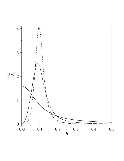
Figure 2: The reduced nondimensional wetting chemical potential $\mu^{(w)}=(1/4)df/dh$, where $f$ is given by Eq. (13). This formula is obtained when $\bar{\gamma}_{p}$ is taken isotropic, $h_{x}$ is taken zero and $\Gamma=0.5$ in Eq. (12b). Also $r=0.1$. Solid line: $m=1$; dash line: $m=3$; dash-dot line: $m=5$.

Now using $h_{0}^{2}/D$ as the time scale, and the small-slope expansion in powers of $\epsilon=|\partial/\partial x|\ll 1$, the asymptotic nondimensional evolution equation (1) reads:

$$h_{t}=B\frac{\partial}{\partial x}\left(P^{(1)}_{\kappa}-\Delta P^{(2)}_{\kappa}+P_{w}\right),$$ (14)

where $B=\Omega^{2}\nu\gamma_{0}/(kTh_{0}^{2})$ is the Mullins coefficient and $P^{(2)}_{\kappa}=-h_{xxxxx}$.

In the exponential model, the terms $P^{(1)}_{\kappa}$ and $P_{w}$ read:

$$P^{(1)}_{\kappa}=\Lambda_{1}h_{xxx}+\Lambda_{2}h_{xx}^{2}h_{x}+\Lambda_{3}h_{xxx}h_{x}^{2}-\exp{\left(-h/r\right)}\left[\left(\Gamma+\Lambda_{1}\right)h_{xxx}+o.t.\right],$$ (15)

$$P_{w}=\frac{\exp{\left(-h/r\right)}}{r}\left[a_{2}h_{xx}h_{x}\left(1-5h_{x}^{2}\right)+r^{-1}h_{x}\left(a_{1}+\left(2a_{3}-3a_{1}\right)h_{x}^{2}+a_{4}h_{x}^{4}\right)\right],$$ (16)

where $\Lambda_{1}=15\epsilon_{\gamma}-1,\ \Lambda_{2}=3-285\epsilon_{\gamma},\ \Lambda_{3}=2-150\epsilon_{\gamma},\ a_{1}=\Gamma-1-\epsilon_{\gamma},\ a_{2}=\Gamma-1-17\epsilon_{\gamma},\ a_{3}=\Gamma-1+3\epsilon_{\gamma},\ a_{4}=\Gamma-1-25\epsilon_{\gamma}$. Notation o.t. (meaning other terms) in the second part of Eq. (15) (which is proportional to the exponent and which stems from wetting interaction), and in the following Eqs. (17), (18) stands for many omitted terms that do not contribute to linear stability. Note that the non-negative $\Lambda_{1}$ signals that the surface energy anisotropy is strong.

In the algebraic model the terms $P^{(1)}_{\kappa}$ and $P_{w}$ read:

$$P^{(1)}_{\kappa} = \frac{h_{xxx}}{2\pi\left(1+(h/r)^{2m}\right)}\left[2\left\{\Gamma+\Lambda_{1}+a_{5}(h/r)^{2m}\right\}\mbox{arctan}\left[\left(h/r\right)^{m}\right]-\right.$$ (17)

$$\left.\pi a_{6}\left(1+(h/r)^{2m}\right)\right]+o.t.,$$

$$P_{w}=\frac{m}{\pi}a_{1}\frac{\left(h/r\right)^{m}h_{x}}{h^{2}\left(1+\left(h/r\right)^{2m}\right)^{2}}\left[1-m+(1+m)(h/r)^{2m}\right]+o.t.,$$ (18)

where $a_{5}=\Gamma-1+15\epsilon_{\gamma}$ and $a_{6}=\Gamma+1-15\epsilon_{\gamma}$.

For computations of the surface evolution (Section IV) we use the parametric equations and the marker particle method. The 1D surface is specified as $\Upsilon(x(u,t),z(u,t))$, where $u$ is the parameter. $x$ and $z$ represent the coordinates of a marker particle on a surface, which are governed by two coupled nondimensional PDEs Sethian1 -HLS :

$$x_{t} = V\frac{1}{g}z_{u},$$ (19a)

$$z_{t} = -V\frac{1}{g}x_{u}.$$ (19b)

Here $V=B\left(\mu^{(\kappa)}_{ss}+\mu^{(w)}_{ss}\right)$ is the normal velocity of the surface, and $g=ds/du=\sqrt{x_{u}^{2}+z_{u}^{2}}$ is the metric function. It can be easily shown that Eqs. (19) are equivalent to dimensionless Eq. (1) when the surface is non-overhanging (a graph of $h=h(x)$ at all times). (Note that in this case $u\equiv x$ and $\partial/\partial s=g^{-1}\partial/\partial u=(1+h_{x}^{2})^{-1/2}\partial/\partial x$.) When the surface develops steep slope, the accurate computation using Eq. (1) requires a fine grid, and when the surface overhangs, Eq. (1) does not make sense. Eqs. (19) and the marker particle method allow to circumvent these problems, and thus this combination is preferred for computation of evolving general surfaces.

III. LINEAR STABILITY ANALYSIS OF THE PLANAR SURFACE

A. Exponential Model

We assume strong anisotropy and linearize Eq. (14) about the equilibrium $h=1$. For the perturbation $\xi(x,t)$ we obtain

$$\xi_{t}=B\left(\Lambda_{1}\xi_{xxxx}+\Delta\xi_{xxxxxx}+\exp{\left(-1/r\right)}\left[r^{-2}a_{1}\xi_{xx}-(\Gamma+\Lambda_{1})\xi_{xxxx}\right]\right).$$ (20)

Taking $\xi=e^{ikx+\omega t}$ gives

$$\omega(k)=B\left[\left(\Lambda_{1}-\exp{\left(-1/r\right)}\left(\Gamma+\Lambda_{1}\right)\right)k^{4}-\Delta k^{6}-\exp{\left(-1/r\right)}r^{-2}a_{1}k^{2}\right].$$ (21)

Note that taking the limit as $r\rightarrow 0$ in Eq. (21) recovers the dispersion relation in the absence of wetting interaction with the substrate, $\omega(k)=B\left[\Lambda_{1}k^{4}-\Delta k^{6}\right]$. It follows from Eq. (21) that the equilibrium surface is unstable ($\omega(k)>0$) to perturbations with the wavenumbers $0<k<k_{c}$, where

$$k_{c}^{2} = (2\Delta)^{-1}\left[\Lambda_{1}-\exp{\left(-1/r\right)}\left(\Gamma+\Lambda_{1}\right)+\right.$$ (22)

$$\left.\left(\left(\Lambda_{1}-\exp{\left(-1/r\right)}\left(\Gamma+\Lambda_{1}\right)\right)^{2}-4\Delta\exp{\left(-1/r\right)}r^{-2}a_{1}\right)^{1/2}\right].$$

Note that the radical at the right-hand side of Eq. (22) always exists when $a_{1}<0$, which turns out to be the necessary condition for a nonwetting film Dwt1 . Fig. 3 shows the sketch of $\omega(k)$. It is interesting that the $k^{2}$-term in Eq. (21) coming from $P_{w}$ (Eq. (16)) makes the film less stable for $a_{1}<0$, but the wetting potential contribution to $P^{(1)}_{\kappa}$ in Eq. (15) makes the surface more stable since the corresponding $k^{4}$-term is negative in Eq. (21). Clearly, due to negative exponent this stabilizing influence is small when $r$ is small.

Figure 3: Sketch of the linear growth rate $\omega(k)$. Perturbations with wavenumbers $0<k<k_{c}$ are unstable and may grow nonlinearly until the film ruptures.

B. Algebraic Model

Eq. (14) gives

$$\omega(k) = B\left[\frac{2\left\{\Gamma+\Lambda_{1}+a_{5}r^{-2m}\right\}A_{0}-\pi a_{6}\left(1+r^{-2m}\right)}{2\pi\left(1+r^{-2m}\right)}k^{4}-\Delta k^{6}-\right.$$ (23)

$$\left.\frac{m\left[1-m+(1+m)r^{-2m}\right]}{\pi r^{m}\left(1+r^{-2m}\right)^{2}}a_{1}k^{2}\right],$$

where $A_{0}=\mbox{arctan}\left[\left(1/r\right)^{m}\right]$.

The cut-off wavenumber is compared in Fig. 4 for both models and the three values of $m$. For $m=1$, $k_{c}$ tends to zero asymptotically, while for $m=3,\ 5$ it becomes zero at $r$ slightly larger than one. Thus the $m=1$ case is qualitatively similar to the exponential model. Comparing the $m=1$ case to the exponential model, it can be seen that for $r<0.5$ the surface is more stable in the former case, and less stable for $r>0.5$. Comparing the $m=3,\ 5$ cases to the exponential model, it can be seen that for small values or $r$ the interval of instability is the same for both models, for intermediate values of $r$ the interval is larger for the algebraic model, and for $r>\sim 1$ the surface governed by the algebraic model is absolutely stable, while there is still a narrow interval of long-wave instability in the exponential model.

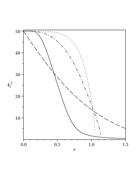
Figure 4: Plots of the square of the critical wavenumber vs. $r$. $\Gamma=0.5,\;\epsilon_{\gamma}=1/12,\;\Delta=0.005$. Solid line: exponential model; dash line: algebraic model with $m=1$; dash-dot line: algebraic model with $m=3$; dot line: algebraic model with $m=5$. (Abrupt termination of the dash-dot and dot lines is the artifact of the plotting software. We confirmed that these lines continue to intersection with the $r$-axis.)

IV. NUMERICAL RESULTS FOR THE LARGE-AMPLITUDE INITIAL DEFORMATION (PINHOLE DEFECT)

In this section the parameters are chosen as follows: $r=0.1,\;\Gamma=0.5,\;\epsilon_{\gamma}=1/12,\;\Delta=0.005$. Following the method of lines approach, Eqs. (19) are discretized in the parameter $u$ using second-order finite differences and the time-stepping is performed by the implicit Runge-Kutta solver RADAU RADAU . Initially $u\equiv x$, but periodically (usually after every few tens of the time steps) the surface is reparametrized so that $u$ becomes the arclength, and the positions of the marker particles are recomputed accordingly. This prevents marker particles from coming too close or too far apart in the course of the surface evolution.

We compute the dynamic morphology and its rate of evolution towards either film rupture or the quasiequilibrium state, which is characterized by the coarsening in time hill-and-valley structure at the both sides of the residual defect, which dissipates with the much slower rate Dwt2 . In Ref. Dwt2 it is shown for the exponential model that for $r$ fixed, the outcome of the evolution (a rupture or a hill-and-valley structure) depends on $\epsilon_{\gamma}$ and the initial condition, i.e. the width and the depth of the pinhole. As will be seen, in the algebraic model the outcome depends also on $m$, which sets the rate of change of the wetting potential. The focus is on the rate of the extension of the pinhole tip in the algebraic model, since the detailed computations for the exponential model are performed in Ref. Dwt2 , and morphologies are similar in both models. Also, since the parameter domain of film rupture is more narrow for the algebraic model, we investigate deep pinholes only.

The initial condition is taken as in Ref. Dwt2 , i.e. the Gaussian curve:

$$z(x,0)=1-d\exp{\left[-\left(\frac{x-5}{w}\right)^{2}\right]},\quad 0\leq x\leq 10,\quad 0<d<1.$$ (24)

Note that the length of the computational domain equals to ten times the unperturbed film height, and the defect is positioned at the center of the domain. Periodic boundary conditions are used.

Figures 5 and 6 show the log-normal plots of the pinhole depth vs time, for $d=0.9$ and $w=2,\;0.15$, respectively. $z_{m}$ is the height of the surface at the tip of the pinhole. The wide pinhole dewets for $m=1$ only. (See Fig. 5. Note that the exponential model predicts faster dewetting.) Wetting potentials with $m=3$ and $m=5$ result in the quasiequilibrium at $0<z_{m}<1$. Quasiequilibrium means that $z_{m}$ (or, equivalently, the depth) changes very slow or not at all, while the rest of the shape changes relatively fast. In the inset, for $m=3$ one can see the onset of the formation of the hill-and-valley structure near the endpoints of the domain; as has been noted in the Introduction, this does not affect the pinhole depth. Interestingly, here the pinhole tip is blunt at quasiequilibrium, while it is sharp in all examples computed for the exponential model Dwt2 .

Figure 5: Kinetics (rate) data for the deep, wide pinhole ($d=0.9,\;w=2$). Line slope equals the rate of the tip evolution. Solid lines: algebraic model. Dash line: exponential model. Inset: Surface shapes at $t=1.8$, for $m=1$ (solid line) and $m=3$ (dash-dot line).

In contrast to the wide pinhole, the narrow pinhole does not dewet even for $m=1$ (Fig. 6) and in all three cases evolves to quasiequilibrium.

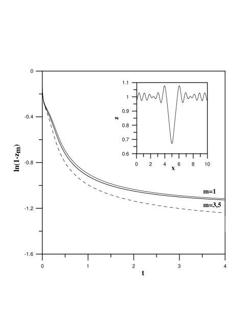
Figure 6: Kinetics data for the deep, narrow pinhole ($d=0.9,\;w=0.15$). Solid lines: algebraic model. Dash line: exponential model. Inset: quasiequilibrium surface shape at $t=4$, for $m=1$.

It must be noted here that stable equilibrium (steady state) solutions have been numerically found in the studies of a nonlinear stress-driven morphological instability of a solid film without wetting interaction, by Spencer & Meiron SM and by Xiang & E XE . The problem under study in this paper differs from the problem studied by these authors in that the instability is driven not by stress but by wetting potential, and the surface energy is anisotropic. These instability mechanisms have different physical origins and the process of morphological evolution in both cases is similar but not the same. In particular, due to the presence of strong surface energy anisotropy the equilibrium solution, when it occurs, is replaced by quasiequilibrium. The latter can be viewed as the locally broken equilibrium. This violation of equilibrium occurs in the surface regions away from the pinhole tip. There, an evolving hill-and-valley structure is energetically favorable because the attraction to the substrate is weak.

Finally, we note that the slight decrease of the initial depth results in the termination of dewetting even for wide pinholes. For instance, Figure 7 shows the case $d=0.7,\;w=2$. As can be seen, there is no dewetting for neither value of $m$. The pinhole tip is attracted to the substrate for a while, but then reverses the direction and will finally stabilize at a quasiequilibrium position. Quasiequilibrium is achieved for the $m=5$ case. For comparison, the exponential model predicts dewetting even for the more shallow pinhole with $d=0.5$ (see Fig. 2(a) in Ref. Dwt2 ).

Figure 7: Kinetics data. $d=0.7,\;w=2$.

To summarize, we contrasted two PDE-based models of dewetting for nonwetting ultrathin single-crystal films. It remains to be seen how these models compare to experiment. Detailed experiments focusing on the dynamics of a single pinhole are yet to be performed. (The published experiments YZSLLHL ; SECS describe very briefly the initial stages of film dewetting and proceed to detailed study of the post-dewetting regimes, i.e. the hole widening, secondary instabilities and material agglomeration.)

ACKNOWLEDGMENT

I thank Brian J. Spencer for pointing out the algebraic decay model to me.

References

- (1) B. Yang, P. Zhang, D.E. Savage, M.G. Lagally, G.-H. Lu, M. Huang, and F. Liu, Phys. Rev. B 72, 235413 (2005).
- (2) P. Sutter, W. Ernst, Y.S. Choi, and E. Sutter, Appl. Phys. Lett. 88, 141924 (2006).
- (3) A. Oron, S. H. Davis, and S. G. Bankoff, Rev. Mod. Phys. 69, 931 (1997).
- (4) R. Seemann, S. Herminghaus, and K. Jacobs, J. Phys.: Condensed Matter 13, 4925 (2001).
- (5) M. Khenner, Phys. Rev. B 77, 165414 (2008).
- (6) M. Khenner, Phys. Rev. B 77, 245445 (2008).
- (7) A.A. Golovin, S.H. Davis, and P.W. Voorhees, Phys. Rev. E 68, 056203 (2003).
- (8) A.A. Golovin, M.S. Levine, T.V. Savina, and S.H. Davis, Phys. Rev. B 70, 235342 (2004).
- (9) T.V. Savina, P.W. Voorhees, and S.H. Davis, J. Appl. Phys. 96, 3127 (2004).
- (10) M.S. Levine, A.A. Golovin, S.H. Davis, and P.W. Voorhees, Phys. Rev. B 75, 205312 (2007).
- (11) C.-h. Chiu and H. Gao, in Thin Films: Stresses and Mechanical Properties V, edited by S.P. Baker, MRS Symposia Proceedings No. 356 (Materials Research Society, Pittsburgh, 1995), p. 33.
- (12) C.-h. Chiu, Phys. Rev. B 69, 165413 (2004).
- (13) Z. Suo and Z. Zhang, Phys. Rev. B 58, 5116 (1998).
- (14) W.W. Mullins, J. Appl. Phys. 28(3), 333 (1957); J. Appl. Phys. 30, 77 (1959).
- (15) B.J. Spencer, Phys. Rev. B 59, 2011 (1999).
- (16) R.V. Kukta and L.B. Freund, J. Mech. Phys. Solids 45, 1835 (1997).
- (17) S. Angenent and M.E. Gurtin, Arch. Rational Mech. Anal. 108, 323 (1989).
- (18) A. Di Carlo, M.E. Gurtin, and P. Podio-Guidugli, SIAM J. Appl. Math. 52, 1111 (1992).
- (19) H.P. Bonzel and E.Preuss, Surface Science 336, 209 (1995).
- (20) B. J. Spencer, Phys. Rev. E 69, 011603 (2004).
- (21) A.A. Golovin, S.H. Davis, and A.A. Nepomnyashchy, Physica D 122, 202 (1998).
- (22) F. Liu and H. Metiu, Phys. Rev. B 48, 5808 (1993).
- (23) J. Stewart and N. Goldenfeld, Phys. Rev. A 46, 6505 (1992).
- (24) C. Herring, in Structure and Properties of Solid Surfaces, Eds. R. Gomer and C.S. Smith (Univ. Chicago Press, Chicago, 1953) 5-81.
- (25) C. Herring, Phys. Rev. 82, 87 (1951).
- (26) J.A. Sethian, Comm. Math. Phys. 101, 487 (1985).
- (27) J.A. Sethian, J. Diff. Geom. 31, 131 (1990).
- (28) R.C. Brower, D.A. Kessler, J. Koplik, and H. Levine, Phys. Rev. A 29, 1335 (1984).
- (29) T.Y. Hou, J.S. Lowengrub, and M.J. Shelley, J. Comput. Phys. 114, 312 (1994).
- (30) E. Hairer and G. Wanner, J. Comput. Appl. Math. 111, 93 (1999).
- (31) B.J. Spencer and D.I. Meiron, Acta Metall. Mater. 42, 3629 (1994).
- (32) Y. Xiang and W. E, J. Appl. Phys. 91, 9414 (2002).