Poisson Geometry of Directed Networks in a Disk

Abstract

We investigate Poisson properties of Postnikov’s map from the space of edge weights of a planar directed network into the Grassmannian. We show that this map is Poisson if the space of edge weights is equipped with a representative of a 6-parameter family of universal quadratic Poisson brackets and the Grasmannian is viewed as a Poisson homogeneous space of the general linear group equipped with an appropriately chosen R-matrix Poisson-Lie structure. We also prove that Poisson brackets on the Grassmannian arising in this way are compatible with the natural cluster algebra structure.

1. Introduction

Directed planar graphs with weighted edges have been widely used in the study of totally nonnegative matrices ([KM, B, BFZ1]). ( Reviews of the area can be found in [FZ2, Fa]. ) In particular, a special kind of such graphs is a convenient tool for visualizing in the $GL_{n}$ case Lusztig type parametrizations of double Bruhat cells [Lu, FZ1]. Each parametrization of this kind is obtained via a factorization of an element of a cell into a product of elementary factors. The standard Poisson-Lie structure on reductive Lie groups is induced by a very simple Poisson bracket on factorization parameters [HKKR, R].

Recently, Postnikov used weighted directed planar graphs to parametrize cells in Grassmannians [P]. The main goal of this paper is to investigate Poisson properties of Postnikov’s parametrization. Using a graphical interpretation of the Poisson-Lie property inspired by the Lusztig parametrization, we introduce a natural family of Poisson brackets on the space of edge weights. These brackets induce a two-parameter family of Poisson brackets on the Grassmannian. Every Poisson bracket in this family is compatible (in the sense of [GSV1, GSV2]) with the cluster algebra on the Grassmannian described in [GSV1, S] and, on the other hand, endows the Grassmannian with a structure of a Poisson homogeneous space with respect to the natural action of the general linear group equipped with an R-matrix Poisson-Lie structure.

This paper is the first in the series devoted to the study of Poisson properties of weighted directed graphs on surfaces. The second paper [GSV3] generalizes results of the current one to graphs in an annulus. In this case, the analogue of Postnikov’s construction leads to a map into the space of loops in the Grassmannian. Natural Poisson brackets on edge weights in this case are intimately connected to trigonometric R-matrix brackets on matrix-valued rational functions. The third paper [GSV4] utilizes particular graphs in an annulus to introduce a cluster algebra structure related to the coordinate ring of the space of normalized rational functions in one variable. This space is birationally equivalent, via the Moser map [M], to any minimal irreducible coadjoint orbit of the group of upper triangular matrices associated with a Coxeter element of the permutation group. In this case, the Poisson bracket compatible with the cluster algebra structure coincides with the quadratic Poisson bracket studied in [FG1, FG2] in the context of Toda flows on minimal orbits. We show that cluster transformations serve as Bäcklund-Darboux transformations between different minimal Toda flows. The fourth paper [GSV5] solves, in the case of graphs in an annulus with one source and one sink, the inverse problem of restoring the weights from the image of the generalized Postnikov map. In the case of arbitrary planar graphs in a disk, this problem was completely solved by Postnikov [P] who proved that for a fixed minimal graph, the space of weights modulo gauge action is birational to its image and described all minimal graphs. To the contrary, already for simplest graphs in an annulus, the corresponding map can only be shown to be finite. In [LP], the inverse problem for the totally nonnegative matrices is solved for a particular type of minimal graphs. In [GSV5] we describe all minimal graphs with one source and one sink.

The paper is organized as follows.

In Section 2, we introduce a notion of a perfect network in a disk and associate with every such network a matrix of boundary measurements. Each boundary measurement is shown to be a rational function in edge weights and admits a subtraction-free rational expression, see Proposition 2.3. In Section 3, we characterize all universal Poisson brackets on the space of edge weights of a given network that respect the natural operation of concatenation of networks, see Proposition 3.1. Furthermore, we establish that the family of universal brackets induces a linear two-parameter family of Poisson brackets on boundary measurement matrices, see Theorem 3.2. This family depends on a mutual location of sources and sinks, but not on the network itself. We provide an explicit description of this family in Theorem 3.3. In Section 4, we start by showing that if the sources and the sinks are not intermixed along the boundary of the disk, one can recover a 2-parametric family of R-matrices and the corresponding R-matrix brackets on $GL_{n}$, see Theorem 4.1. Next, the boundary measurement map defined by a network with $k$ sources and $n-k$ sinks is extended to the Grassmannian boundary measurement map into the Grassmannian $G_{k}(n)$. The Poisson family on boundary measurement matrices allows us to equip the Grassmannian with a two-parameter family of Poisson brackets ${\mathcal{P}}_{\alpha,\beta}$ in such a way that for any choice of a universal Poisson bracket on edge weights there is a unique member of ${\mathcal{P}}_{\alpha,\beta}$ that makes the Grassmannian boundary measurement map Poisson, see Theorem 4.3. This latter family depends only on the number of sources and sinks and does not depend on their mutual location. Finally, we give an interpretation of the natural $GL_{n}$ action on $G_{k}(n)$ in terms of networks and establish that every member of the Poisson family ${\mathcal{P}}_{\alpha,\beta}$ on $G_{k}(n)$ makes $G_{k}(n)$ into a Poisson homogeneous space of $GL_{n}$ equipped with the above described R-matrix bracket, see Theorem 4.8. In Section 5, we review the construction of the cluster algebra structure on an open cell in the Grassmannian given in [GSV1]. We then introduce face weights and use them to show that every member of the Poisson family ${\mathcal{P}}_{\alpha,\beta}$ is compatible with this cluster algebra structure, see Theorem 5.4.

2. Perfect planar networks and boundary measurements

2.1. Networks, paths and weights

Let $G=(V,E)$ be a directed planar graph with no loops and parallel edges drawn inside a disk (and considered up to an isotopy) with the vertex set $V$ and the edge set $E$. Exactly $n$ of its vertices are located on the boundary circle of the disk. They are labelled counterclockwise $b_{1},\dots,b_{n}$ and called boundary vertices; occasionally we will write $b_{0}$ for $b_{n}$ and $b_{n+1}$ for $b_{1}$. Each boundary vertex is marked as a source or a sink. A source is a vertex with exactly one outcoming edge and no incoming edges. Sinks are defined in the same way, with the direction of the single edge reversed. The number of sources is denoted by $k$, and the corresponding set of indices, by $I\subset[1,n]$; the set of the remaining $m=n-k$ indices is denoted by $J$. All the internal vertices of $G$ have degree $3$ and are of two types: either they have exactly one incoming edge, or exactly one outcoming edge. The vertices of the first type are called (and shown on figures) white, those of the second type, black.

Let $x_{1},\dots,x_{d}$ be independent variables. A perfect planar network $N=(G,w)$ is obtained from $G$ as above by assigning a weight $w_{e}\in{\mathbb{Z}}(x_{1},\dots,x_{d})$ to each edge $e\in E$. In what follows we occasionally write “network” instead of “perfect planar network”. Each network defines a rational map $w:{\mathbb{R}}^{d}\to{\mathbb{R}}^{|E|}$; the space of edge weights ${\mathcal{E}}_{N}$ is defined as the intersection of the image of $({\mathbb{R}}\setminus 0)^{d}$ under $w$ with $({\mathbb{R}}\setminus 0)^{|E|}$. In other words, a point in ${\mathcal{E}}_{N}$ is a graph $G$ as above with edges weighted by nonzero reals obtained by specializing the variables $x_{1},\dots,x_{d}$ in the expressions for $w_{e}$ to nonzero values.

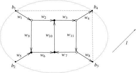
Figure 1. A perfect planar network in a disk

An example of a perfect planar network is shown in Fig. 1. It has two sources: $b_{1}$ and $b_{2}$, and two sinks $b_{3}$ and $b_{4}$. Each edge $e_{i}$ is labelled by its weight. The weights depend on four independent variables $x_{1},x_{2},x_{3},x_{4}$ and are given by

$$w_{1}=x_{1}^{2}/(x_{2}+1),\qquad w_{2}=x_{2},\qquad w_{3}=x_{2}+1,\qquad w_{4}=x_{1}+x_{3},$$

$$w_{5}=x_{3},\qquad w_{6}=x_{3},\qquad w_{7}=x_{3},\qquad w_{8}=x_{4},$$

$$w_{9}=1,\qquad w_{10}=1,\qquad w_{11}=1.$$

The space of edge weights is the 4-dimensional subvariety in $({\mathbb{R}}\setminus 0)^{11}$ given by equations $w_{1}w_{3}=(w_{4}-w_{5})^{2}$, $w_{3}=w_{2}+1$, $w_{5}=w_{6}=w_{7}$, $w_{9}=w_{10}=w_{11}=1$ and condition $w_{3}\neq 1$.

A path $P$ in $N$ is an alternating sequence $(v_{1},e_{1},v_{2},\dots,e_{r},v_{r+1})$ of vertices and edges such that $e_{i}=(v_{i},v_{i+1})$ for any $i\in[1,r]$. Sometimes we omit the names of the vertices and write $P=(e_{1},\dots,e_{r})$. A path is called a cycle if $v_{r+1}=v_{1}$ and a simple cycle if additionally $v_{i}\neq v_{j}$ for any other pair $i\neq j$.

To define the weights of the paths we need the following construction. Consider a closed oriented polygonal plane curve $C$. Let $e^{\prime}$ and $e^{\prime\prime}$ be two consequent oriented segments of $C$, and let $v$ be their common vertex. We assume for simplicity that for any such pair $(e^{\prime},e^{\prime\prime})$, the cone spanned by $e^{\prime}$ and $e^{\prime\prime}$ is not a line; in other words, if $e^{\prime}$ and $e^{\prime\prime}$ are collinear, then they have the same direction. Observe that since $C$ is not necessary simple, there might be other edges of $C$ incident to $v$ (see Figure 2 below). Let $l$ be an arbitrary oriented line. Define $c_{l}(e^{\prime},e^{\prime\prime})\in{\mathbb{Z}}/2{\mathbb{Z}}$ in the following way: $c_{l}(e^{\prime},e^{\prime\prime})=1$ if the directing vector of $l$ belongs to the interior of the cone spanned by $e^{\prime}$ and $e^{\prime\prime}$ and $c_{l}(e^{\prime},e^{\prime\prime})=0$ otherwise (see Figure 2 for examples). Define $c_{l}(C)$ as the sum of $c_{l}(e^{\prime},e^{\prime\prime})$ over all pairs of consequent segments in $C$. It follows immediately from Theorem 1 in [GrSh] that $c_{l}(C)$ does not depend on $l$, provided $l$ is not collinear to any of the segments in $C$. The common value of $c_{l}(C)$ for different choices of $l$ is denoted by $c(C)$ and called the concordance number of $C$. In fact, $c(C)$ equals $\mod 2$ the rotation number of $C$; the definition of the latter is similar, but more complicated.

Figure 2. To the definition of the concordance number: $c_{l}(e_{1},e_{2})=c_{l}(e_{5},e_{2})=0$; $c_{l}(e_{2},e_{3})=1,c_{l}(e_{2},e_{6})=0$; $c_{l}(e_{6},e_{7})=1,c_{l}(e_{7},e_{8})=0$

In what follows we assume without loss of generality that $N$ is drawn in such a way that all its edges are straight line segments and all internal vertices belong to the interior of the convex hull of the boundary vertices. Given a path $P$ between a source $b_{i}$ and a sink $b_{j}$, we define a closed polygonal curve $C_{P}$ by adding to $P$ the path between $b_{j}$ and $b_{i}$ that goes counterclockwise along the boundary of the convex hull of all the boundary vertices of $N$. Finally the weight of $P$ is defined as

$$w_{P}=(-1)^{c(C_{P})-1}\prod_{e\in P}w_{e}.$$

The weight of an arbitrary cycle in $N$ is defined in the same way via the concordance number of the cycle.

If edges $e_{i}$ and $e_{j}$ in $P$ coincide and $i<j$, the path $P$ can be decomposed into the path $P^{\prime}=(e_{1},\dots,e_{i-1},e_{i}=e_{j},e_{j+1},\dots,e_{r})$ and the cycle $C^{0}=(e_{i},e_{i+1},\dots,e_{j-1})$. Clearly, $c(C_{P})=c(C_{P^{\prime}})+c(C^{0})$, and hence

$$w_{P}=-w_{P^{\prime}}w_{C^{0}}.$$ (2.1)

Example 2.1.

Consider the path $P=(e_{1},e_{2},e_{3},e_{11},e_{7},e_{10},e_{3},e_{11},e_{8})$ in Figure 1. Choose $l$ as shown in the Figure; $l$ is neither collinear with the edges of $P$ nor with the relevant edges of the convex hull of boundary vertices (shown by dotted lines). Clearly, $c_{l}(e^{\prime},e^{\prime\prime})=0$ for all pairs of consecutive edges of $C_{P}$ except for the pairs $(e_{10},e_{3})$ and $(e_{8},\bar{e})$, where $\bar{e}$ is the additional edge joining $b_{3}$ and $b_{4}$. So, $c(C_{P})=0$, and hence $w_{P}=-w_{1}w_{2}w_{3}^{2}w_{7}w_{8}w_{10}w_{11}^{2}$. The same result can be obtained by decomposing $P$ into the path $P^{\prime}=(e_{1},e_{2},e_{3},e_{11},e_{8})$ and the cycle $C^{0}=(e_{3},e_{11},e_{7},e_{10})$.

Remark 2.2.

Instead of closed polygonal curves $C_{P}$, one can use curves $C^{*}_{P}$ obtained by adding to $P$ the path between $b_{j}$ and $b_{i}$ that goes clockwise along the boundary of the convex hull of all the boundary vertices of $N$. It is a simple exercise to prove that the concordance numbers of $C_{P}$ and $C^{*}_{P}$ coincide. Therefore, the weight of a path can be defined also as

$$w_{P}=(-1)^{c(C^{*}_{P})-1}\prod_{e\in P}w_{e}.$$

2.2. Boundary measurements

Given a perfect planar network as above, a source $b_{i}$, $i\in I$, and a sink $b_{j}$, $j\in J$, we define the boundary measurement $M(i,j)$ as the sum of the weights of all paths starting at $b_{i}$ and ending at $b_{j}$. Clearly, the boundary measurement thus defined is a formal infinite series in variables $w_{e}$, $e\in E$. However, this series possesses certain nice propetsies.

Recall that a formal power series $g\in{\mathbb{Z}}[[w_{e},e\in E]]$ is called a rational function if there exist polynomials $p,q\in{\mathbb{Z}}[w_{e},e\in E]$ such that $p=qg$ in ${\mathbb{Z}}[[w_{e},e\in E]]$. In this case we write $g=p/q$. For example, $1-z+z^{2}-z^{3}+\dots=(1+z)^{-1}$ in ${\mathbb{Z}}[[z]]$. Besides, we say that $g$ admits a subtraction-free rational expression if it can be written as a ratio of two polynomials with nonnegative coefficients. For example, $x^{2}-xy+y^{2}$ admits a subtraction-free rational expression since it can be written as $(x^{3}+y^{3})/(x+y)$.

The following result was proved in [P][Lemma 4.3] and further generalized in [T], but we will present an alternative proof to illustrate the method that will be used in other proofs below.

Proposition 2.3.

Let $N$ be a perfect planar network in a disk, then each boundary measurement in $N$ is a rational function in the weights $w_{e}$ admitting a subtraction-free rational expression.

Proof.

We prove the claim by induction on the number of internal vertices. The base of induction is the case when there are no internal vertices at all, and hence each edge connects a source and a sink; in this case the statement of the proposition holds trivially.

Assume that $N$ has $r$ internal vertices. Consider a specific boundary measurement $M(i,j)$. The claim concerning $M(i,j)$ is trivial if $b_{j}$ is the neighbor of $b_{i}$. In the remaining cases $b_{i}$ is connected by an edge $e_{0}$ to its only neighbor in $G$, which is either white or black.

Assume first that the neighbor of $b_{i}$ is a white vertex $v$. Create a new network ${\widetilde{N}}$ by deleting $b_{i}$ and the edge $(b_{i},v)$ from $G$, splitting $v$ into $2$ sources $b_{i_{v}^{\prime}},b_{i_{v}^{\prime\prime}}$ (so that $i-1\prec i_{v}^{\prime}\prec i_{v}^{\prime\prime}\prec i+1$ in the counterclockwise order) and replacing the edges $e_{1}=(v,v^{\prime})$ and $e_{2}=(v,v^{\prime\prime})$ by $(b_{i_{v}^{\prime}},v^{\prime})$ and $(b_{i_{v}^{\prime\prime}},v^{\prime\prime})$, respectively, both of weight 1 (see Figure 3). Clearly, to any path $P$ from $b_{i}$ to $b_{j}$ corresponds either a path $P^{\prime}$ from $b_{i^{\prime}_{v}}$ to $b_{j}$ or a path $P^{\prime\prime}$ from $b_{i^{\prime\prime}_{v}}$ to $b_{j}$. Moreover, $c(C_{P})=c(C_{P^{\prime}})=c(C_{P^{\prime\prime}})$. Therefore

$$M(i,j)=w_{e_{0}}(w_{e_{1}}{\widetilde{M}}({i^{\prime}_{v}},j)+w_{e_{2}}{\widetilde{M}}({i^{\prime\prime}_{v}},j)),$$

where ${\widetilde{M}}$ means that the measurement is taken in ${\widetilde{N}}$. Observe that the number of internal vertices in ${\widetilde{N}}$ is $r-1$, hence the claim follows from the above relation by induction.

Figure 3. Splitting a white vertex

Assume now that the neighbor of $b_{i}$ is a black vertex $u$. Denote by $u_{+}$ the unique vertex in $G$ such that $(u,u_{+})\in E$, and by $u_{-}$ the neighbor of $u$ distinct from $u_{+}$ and $b_{i}$. Create a new network ${\widehat{N}}$ by deleting $b_{i}$ and the edge $(b_{i},u)$ from $G$, splitting $u$ into one new source $b_{i_{u}}$ and one new sink $b_{j_{u}}$ (so that either $i-1\prec i_{u}\prec j_{u}\prec i+1$ or $i-1\prec j_{u}\prec i_{u}\prec i+1$ in the counterclockwise order) and replacing the edges $e_{+}=(u,u_{+})$ and $e_{-}=(u_{-},u)$ by new edges $\hat{e}_{+}$ and $\hat{e}_{-}$ in the same way as in the previous case, see Figure 4.

Let us classify the paths from $b_{i}$ to $b_{j}$ according to the number of times they traverse $e_{+}$. Similarly to the previous case, the total weight of the paths traversing $e_{+}$ only once is given by $w_{e_{0}}w_{e_{+}}{\widehat{M}}({i_{v}},j)$, where ${\widehat{M}}$ means that the measurement is taken in ${\widehat{N}}$. Any path $P$ traversing $e_{+}$ exactly twice can be represented as $P=(e_{0},e_{+},P_{1},e_{-},e_{+},P_{2})$ for some path ${\widehat{P}}_{1}=(\hat{e}_{+},P_{1},\hat{e}_{-})$ from $i_{u}$ to $j_{u}$ in ${\widehat{N}}$ and a path ${\widehat{P}}_{2}=(\hat{e}_{+},P_{2})$ from $i_{u}$ to $b_{j}$ in ${\widehat{N}}$. Clearly, $C_{1}=(e_{+},P_{1},e_{-})$ is a cycle in $N$, and $c(C_{1})=c(C_{{\widehat{P}}^{1}})$. Besides, $c(C_{P^{\prime}})=c(C_{{\widehat{P}}_{2}})$ for $P^{\prime}=(e_{0},e_{+},P_{2})$. Therefore, by (2.1), $w_{P}=-w_{C_{1}}w_{P^{\prime}}$. Taking into account that $w_{C_{1}}=w_{e_{-}}w_{e_{+}}w_{{\widehat{P}}_{1}}$ and $w_{P^{\prime}}=w_{e_{0}}w_{e_{+}}w_{{\widehat{P}}_{2}}$, we see that the total contribution of all paths traversing $e_{+}$ exactly twice to $M(i,j)$ equals

$$-w_{e_{0}}w_{e_{+}}{\widehat{M}}({i_{u}},{j})w_{e_{-}}w_{e_{+}}{\widehat{M}}({i_{u}},j_{u}).$$

In general, the total contribution of all paths traversing $e_{+}$ exactly $s+1$ times to $M(i,j)$ equals

$$(-1)^{s}w_{e_{0}}w_{e_{+}}{\widehat{M}}({i_{u}},{j})(w_{e_{-}}w_{e_{+}}{\widehat{M}}({i_{u}},j_{u}))^{s}.$$

Therefore, we find

$$M(i,j)=\frac{w_{e_{0}}w_{e_{+}}{\widehat{M}}({i_{u}},{j})}{1+w_{e_{-}}w_{e_{+}}{\widehat{M}}({i_{u}},j_{u})}$$ (2.2)

and the claim follows by induction, since the number of internal vertices in ${\widehat{N}}$ is $r-1$. ∎

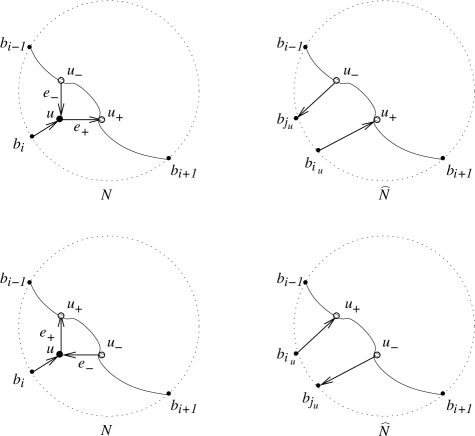
Figure 4. Splitting a black vertex: cases $i-1\prec i_{u}\prec j_{u}\prec i+1$ (upper part) and $i-1\prec j_{u}\prec i_{u}\prec i+1$ (lower part)

Boundary measurements can be organized into a $k\times m$ boundary measurement matrix $M_{N}$ in the following way. Let $I=\{i_{1}<i_{2}<\dots<i_{k}\}$ and $J=\{j_{1}<j_{2}<\dots<j_{m}\}$. We define $M_{N}=(M_{pq})$, $p\in[1,k]$, $q\in[1,m]$, where $M_{pq}=M({i_{p}},{j_{q}})$. Each network $N$ defines a rational map ${\mathcal{E}}_{N}\to\operatorname{Mat}_{k,m}$ given by $M_{N}$ and called the boundary measurement map corresponding to $N$. Here and below $\operatorname{Mat}_{k,m}$ denotes the space of $k\times m$ matrices.

Example 2.4.

Consider the network shown in Figure 1. The corresponding boundary measurement matrix is a $2\times 2$ matrix given by

$$\begin{pmatrix}\dfrac{w_{3}w_{4}w_{5}w_{6}w_{10}}{1+w_{3}w_{7}w_{10}w_{11}}&\dfrac{w_{3}w_{5}w_{6}w_{8}w_{11}}{1+w_{3}w_{7}w_{10}w_{11}}\\ \\ \dfrac{w_{1}w_{3}w_{4}(w_{2}+w_{6}w_{9}w_{10})}{1+w_{3}w_{7}w_{10}w_{11}}&\dfrac{w_{1}w_{3}w_{8}w_{11}(w_{2}+w_{6}w_{9}w_{10})}{1+w_{3}w_{7}w_{10}w_{11}}\end{pmatrix}.$$

3. Poisson structures on the space of edge weights and induced Poisson structures on $\operatorname{Mat}_{k,m}$

3.1. Network concatenation and the standard Poisson-Lie structure

A natural operation on networks is their concatenation, which consists, roughly speaking, in gluing some sinks/sources of one network to some of the sources/sinks of the other. We expect any Poisson structure associated with networks to behave naturally under concatenation. To obtain from two planar networks a new one by concatenation, one needs to select a segment from the boundary of each disk and identify these segments via a homeomorphism in such a way that every sink (resp. source) contained in the selected segment of the first network is glued to a source (resp. sink) of the second network. We can then erase the common piece of the boundary along which the gluing was performed and identify every pair of glued edges in the resulting network with a single edge of the same orientation and with the weight equal to the product of two weights assigned to the two edges that were glued.

As an illustration, let us review a particular but important case, in which sources and sinks of the network do not interlace. In this case, it is more convenient to view the network as located in a square rather than in a disk, with all sources located on the left side and sinks on the right side of the square. It will be also handy to label sources (resp. sinks) $1$ to $k$ (resp. $1$ to $m$) going from the bottom to the top. This results in a different way of recording boundary measurements into a matrix. Namely, if $M$ is the boundary measurements matrix we defined earlier, then now we associate with the network the matrix $A=MW_{0}$, where $W_{0}=(\delta_{i,m+1-j})_{i,j=1}^{m}$ is the matrix of the longest permutation $w_{0}$.

We can now concatenate two networks of this kind, one with $k$ sources and $m$ sinks and another with $m$ sources and $l$ sinks, by gluing the sinks of the former to the sources of the latter. If $A_{1}$, $A_{2}$ are $k\times m$ and $m\times l$ matrices associated with the two networks, then the matrix associated with their concatenation is $A_{1}A_{2}$. Note that this “visualization” of the matrix multiplication is particularly relevant when one deals with factorization of matrices into products of elementary bidiagonal matrices. Indeed, a $n\times n$ diagonal matrix $\operatorname{diag}(d_{1},\ldots,d_{n})$ and elementary bidiagonal matrices $E^{-}_{i}(l):=\mathbf{1}+le_{i,i-1}$ and $E^{+}_{j}(u):=\mathbf{1}+ue_{j-1,j}$ correspond to planar networks shown in Figure 5 a, b and c, respectively; all weights not shown explicitly are equal to 1.

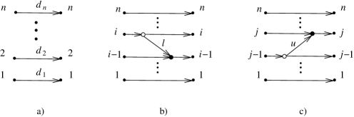
Figure 5. Three networks used in matrix factorization

The construction of Poisson structures we are about to present is motivated by the way in which the network representation of the bidiagonal factorization reflects the standard Poisson-Lie structure on $SL_{n}$. We need to recall some facts about Poisson-Lie groups (see, e.g.[ReST]).

Let ${\mathcal{G}}$ be a Lie group equipped with a Poisson bracket ${\{\cdot,\cdot\}}$. ${\mathcal{G}}$ is called a Poisson-Lie group if the multiplication map

$${\mathfrak{m}}:{\mathcal{G}}\times{\mathcal{G}}\ni(x,y)\mapsto xy\in{\mathcal{G}}$$

is Poisson. Perhaps, the most important class of Poisson-Lie groups is the one associated with classical R-matrices.

Let $\mathfrak{g}$ be a Lie algebra of ${\mathcal{G}}$. Assume that $\mathfrak{g}$ is equipped with a nondegenerate invariant bilinear form $(\ ,\ )$. An element $R\in\operatorname{End}(\mathfrak{g})$ is a classical R-matrix if it is a skew-symmetric operator that satisfies the modified classical Yang-Baxter equation (MCYBE)

$$[R(\xi),R(\eta)]-R\left([R(\xi),\eta]\ +\ [\xi,R(\eta)]\right)=-[\xi,\eta]\ .$$ (3.1)

Given a classical R-matrix $R$, ${\mathcal{G}}$ can be endowed with a Poisson-Lie structure as follows. Let $\nabla f,\nabla^{\prime}f$ be the right and the left gradients for a function $f\in C^{\infty}({\mathcal{G}})$:

$$(\nabla f(x),\xi)=\frac{d}{dt}f(\exp{(t\xi)}x)|_{t=0},\qquad(\nabla^{\prime}f(x),\xi)=\frac{d}{dt}f(x\exp{(t\xi)})|_{t=0}\ .$$ (3.2)

Then the bracket given by

$$\{f_{1},f_{2}\}=\frac{1}{2}(R(\nabla^{\prime}f_{1}),\nabla^{\prime}f_{2})-\frac{1}{2}(R(\nabla f_{1}),\nabla f_{2})\$$

is a Poisson-Lie bracket on ${\mathcal{G}}$ called the Sklyanin bracket.

We are interested in the case ${\mathcal{G}}=SL_{n}$ and $\mathfrak{g}=sl_{n}$ equipped with the trace-form

$$(\xi,\eta)=\operatorname{Tr}(\xi\eta)\ .$$

Then the right and left gradients (3.2) are

$$\nabla f(x)=x\ \mbox{grad}f(x)\ ,\qquad\nabla^{\prime}f(x)=\mbox{grad}f(x)\ x\ ,$$

where

$$\mbox{grad}f(x)=\left(\frac{\partial f}{\partial x_{ji}}\right)_{i,j=1}^{n}\ ,$$

and the Sklyanin bracket becomes

$$\{f_{1},f_{2}\}_{SL_{n}}(x)=\\ \frac{1}{2}(R(\mbox{grad}f_{1}(x)\ x),\mbox{grad}f_{2}(x)\ x)-\frac{1}{2}(R(x\ \mbox{grad}f_{1}(x)),x\ \mbox{grad}f_{2}(x))\ .$$ (3.3)

Every $\xi\in\mathfrak{g}$ can be uniquely decomposed as

$$\xi=\xi_{-}+\xi_{0}+\xi_{+}\ ,$$

where $\xi_{+}$ and $\xi_{-}$ are strictly upper and lower triangular and $\xi_{0}$ is diagonal. The simplest classical R-matrix on $sl_{n}$ is given by

$$R_{0}(\xi)=\xi_{+}-\xi_{-}=\left(\operatorname{sign}(j-i)\xi_{ij}\right)_{i,j=1}^{n}.$$ (3.4)

Substituting into (3.3) $R=R_{0}$ we obtain , for matrix entries $x_{ij},\ x_{i^{\prime}j^{\prime}}$,

$$\{x_{ij},x_{i^{\prime}j^{\prime}}\}_{SL_{n}}=\frac{1}{2}\left(\operatorname{sign}(i^{\prime}-i)+\operatorname{sign}(j^{\prime}-j)\right)x_{ij^{\prime}}x_{i^{\prime}j}\ .$$ (3.5)

The bracket (3.3) extends naturally to a Poisson bracket on the space $\operatorname{Mat}_{n}$ of $n\times n$ matrices.

For example, the standard Poisson-Lie structure on

$$SL_{2}=\left\{\left(\begin{array}[]{cc}a&b\\ c&d\end{array}\right)\ :\ ad-bc=1\ \right\}$$

is described by the relations

$$\{a,b\}_{SL_{2}}=\frac{1}{2}ab,\quad\{a,c\}_{SL_{2}}=\frac{1}{2}ac,\quad\{a,d\}_{SL_{2}}=bc,$$

$$\{c,d\}_{SL_{2}}=\frac{1}{2}cd,\quad\{b,d\}_{SL_{2}}=\frac{1}{2}bd,\quad\{b,c\}_{SL_{2}}=0\ ,$$

which, when restricted to upper and lower Borel subgroups of $SL_{2}$

$$B_{+}=\left\{\begin{pmatrix}d&c\\ 0&d^{-1}\end{pmatrix}\right\},\qquad B_{-}=\left\{\begin{pmatrix}d&0\\ c&d^{-1}\end{pmatrix}\right\}$$

have an especially simple form

$$\{d,c\}=\frac{1}{2}dc.$$

The latter Poisson brackets can be used to give an alternative characterization of the standard Poisson-Lie structure on $SL_{n}$. Namely, define the canonical embedding $\rho_{i}:SL_{2}\to SL_{n}$ ($i\in[1,n-1]$) that maps $SL_{2}$ into $SL_{n}$ as a diagonal $2\times 2$ block occupying rows and columns $i$ and $i+1$. Then the standard Poisson-Lie structure on $SL_{n}$ is defined uniquely (up to a scalar multiple) by the requirement that restrictions of $\rho_{i}$ to $B_{\pm}$ are Poisson.

Note that the network that represents $\rho_{i}(B_{-})$ looks like the second network in the figure above with the weights $d,d^{-1}$ and $c$ attached to edges $(i-1)\to(i-1)$, $i\to i$ and $i\to(i-1)$ resp., while the network that represents $\rho_{j}(B_{+})$ looks like the third network in the figure above with the weights $d,d^{-1}$ and $c$ attached to edges $(j-1)\to(j-1)$, $j\to j$ and $(j-1)\to j$ resp. Concatenation of several networks $N_{1},\cdots,N_{r}$, $r=n(n-1)$, of these two kinds, with appropriately chosen order and with each diagram having its own pair of nontrivial weights $c_{i},d_{i}$, describes a generic element of $SL_{n}$ (see, e.g. [Fa]). An example of such a network is given by Figure 6.

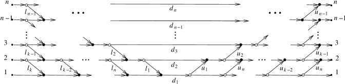
Figure 6. Generic planar network

On the other hand, due to the Poisson-Lie property, the Poisson structure on $SL_{n}$ is inherited from simple Poisson brackets for parameters $c_{i},d_{i}$, which can be described completely in terms of networks: (i) the bracket of any two parameters is equal to their product times a constant; (ii) this constant is equal to zero unless the corresponding edges have a common source/sink; (iii) the constant equals $\pm\frac{1}{2}$ if the corresponding edges follow one another around the source/sink in the counterclockwise direction. The corresponding Poisson-Lie structure on $GL_{n}$ is obtained by requiring the determinant to be a Casimir function.

This example motivates conditions we impose below on a natural Poisson structure associated with a 3-valent planar directed network.

3.2. Poisson structures on the space of edge weights

Let G be a directed planar graph in a disk as described in Section 2.1. A pair $(v,e)$ is called a flag if $v$ is an endpoint of $e$. To each internal vertex $v$ of $G$ we assign a 3-dimensional space ${({\mathbb{R}}\setminus 0)}_{v}^{3}$ with coordinates $x_{v}^{1},x_{v}^{2},x_{v}^{3}$. We equip each ${({\mathbb{R}}\setminus 0)}_{v}^{3}$ with a Poisson bracket $\{\cdot,\cdot\}_{v}$. It is convenient to assume that the flags involving $v$ are labelled by the coordinates, as shown in Figure 7.

Figure 7. Edge labelling for ${({\mathbb{R}}\setminus 0)}_{v}^{3}$

Besides, to each boundary vertex $b_{j}$ of $G$ we assign a 1-dimensional space ${({\mathbb{R}}\setminus 0)}_{j}$ with the coordinate $x_{j}^{1}$ (in accordance with the above convention, this coordinate labels the unique flag involving $b_{j}$). Define ${\mathcal{R}}$ to be the direct sum of all the above spaces; thus, the dimension of ${\mathcal{R}}$ equals twice the number of edges in $G$. Note that ${\mathcal{R}}$ is equipped with a Poisson bracket $\{\cdot,\cdot\}_{\mathcal{R}}$, which is defined as the direct sum of the brackets $\{\cdot,\cdot\}_{v}$; that is, $\{x,y\}_{\mathcal{R}}=0$ whenever $x$ and $y$ are not defined on the same ${({\mathbb{R}}\setminus 0)}_{v}^{3}$. We say that the bracket $\{\cdot,\cdot\}_{\mathcal{R}}$ is universal if each of $\{\cdot,\cdot\}_{v}$ depends only on the color of the vertex $v$.

Define the weights $w_{e}$ by

$$w_{e}=x^{i}_{v}x^{j}_{u},$$ (3.6)

provided the flag $(v,e)$ is labelled by $x^{i}_{v}$ and the flag $(u,e)$ is labelled by $x^{j}_{u}$. In other words, the weight of an edge is defined as the product of the weights of the two flags involving this edge. Therefore, in this case the space of edge weights ${\mathcal{E}}_{N}$ coincides with the entire ${({\mathbb{R}}\setminus 0)}^{|E|}$, and the weights define a weight map $w{:\ }{({\mathbb{R}}\setminus 0)}^{d}\to{({\mathbb{R}}\setminus 0)}^{|E|}$. We require the pushforward of $\{\cdot,\cdot\}_{\mathcal{R}}$ to ${({\mathbb{R}}\setminus 0)}^{|E|}$ by the weight map to be a well defined Poisson bracket; this can be regarded as an analog of the Poisson–Lie property for groups.

Proposition 3.1.

Universal Poisson brackets $\{\cdot,\cdot\}_{\mathcal{R}}$ such that the weight map $w$ is Poisson form a $6$-parametric family defined by relations

$$\{x^{i}_{v},x^{j}_{v}\}_{v}=\alpha_{ij}x^{i}_{v}x^{j}_{v},\quad i,j\in[1,3],i\neq j,$$ (3.7)

at each white vertex $v$ and

$$\{x^{i}_{v},x^{j}_{v}\}_{v}=\beta_{ij}x^{i}_{v}x^{j}_{v},\quad i,j\in[1,3],i\neq j,$$ (3.8)

at each black vertex $v$.

Proof.

Indeed, let $v$ be a white vertex, and let $e=(v,u)$ and $\bar{e}=(v,\bar{u})$ be the two outcoming edges. By definition, there exist $i,j,k,l\in[1,3]$, $i\neq j$, such that $w_{e}=x_{v}^{i}x_{u}^{k}$, $w_{\bar{e}}=x_{v}^{j}x_{\bar{u}}^{l}$. Therefore,

$$\{w_{e},w_{\bar{e}}\}_{N}=\{x_{v}^{i}x_{u}^{k},x_{v}^{j}x_{\bar{u}}^{l}\}_{\mathcal{R}}=x_{u}^{k}x_{\bar{u}}^{l}\{x_{v}^{i},x_{v}^{j}\}_{v},$$

where $\{\cdot,\cdot\}_{N}$ stands for the pushforward of $\{\cdot,\cdot\}_{\mathcal{R}}$. Recall that the Poisson bracket in ${({\mathbb{R}}\setminus 0)}_{v}^{3}$ depends only on $x_{v}^{1}$, $x_{v}^{2}$ and $x_{v}^{3}$. Hence the only possibility for the right hand side of the above relation to be a function of $w_{e}$ and $w_{\bar{e}}$ occurs when $\{x^{i}_{v},x^{j}_{v}\}_{v}=\alpha_{ij}x^{i}_{v}x^{j}_{v}$, as required.

Black vertices are treated in the same way. ∎

Let $v$ be a white vertex. A local gauge transformation at $v$ is a transformation ${({\mathbb{R}}\setminus 0)}_{v}^{3}\to{({\mathbb{R}}\setminus 0)}_{v}^{3}$ defined by $(x_{v}^{1},x_{v}^{2},x_{v}^{3})\mapsto(\bar{x}_{v}^{1}=x_{v}^{1}t_{v},\bar{x}_{v}^{2}=x_{v}^{2}t_{v}^{-1},\bar{x}_{v}^{3}=x_{v}^{3}t_{v}^{-1})$, where $t_{v}$ is a Laurent monomial in $x_{v}^{1}$, $x_{v}^{2}$, $x_{v}^{3}$. A local gauge transformation at a black vertex is defined by the same formulas, with $t_{v}$ replaced by $t_{v}^{-1}$.

A global gauge transformation $t{:\ }{\mathcal{R}}\to{\mathcal{R}}$ is defined by applying a local gauge transformation $t_{v}$ at each vertex $v$. The composition map $w\circ t$ defines a network $tN$; the graph of $tN$ coincides with the graph of $N$, and the weight $w^{t}_{e}$ of an edge $e=(u,v)$ is given by $w^{t}_{e}=t_{v}w_{e}t_{u}^{-1}$. Therefore, the weights of the same path in $N$ and $tN$ coincide. It follows immediately that

$$M_{tN}\circ w\circ t=M_{N}\circ w,$$ (3.9)

provided both sides of the equality are well defined.

3.3. Induced Poisson structures on $\operatorname{Mat}_{k,m}$

Our next goal is to look at Poisson properties of the boundary measurement map. Fix an arbitrary partition $I\cup J=[1,n]$, $I\cap J=\varnothing$, and let $k=|I|$, $m=n-k=|J|$. Let $\operatorname{Net}_{I,J}$ stand for the set of all perfect planar networks in a disk with the sources $b_{i}$, $i\in I$, sinks $b_{j}$, $j\in J$, and edge weights $w_{e}$ defined by (3.6). We assume that the space of edge weights ${\mathcal{E}}_{N}={({\mathbb{R}}\setminus 0)}^{|E|}$ is equipped with the Poisson bracket $\{\cdot,\cdot\}_{N}$ obtained as the pushforward of the 6-parametric family $\{\cdot,\cdot\}_{\mathcal{R}}$ described in Proposition 3.1.

Theorem 3.2.

There exists a $2$-parametric family of Poisson brackets on $\operatorname{Mat}_{k,m}$ with the following property: for any choice of parameters $\alpha_{ij}$, $\beta_{ij}$ in (3.7), (3.8) this family contains a unique Poisson bracket on $\operatorname{Mat}_{k,m}$ such that for any network $N\in\operatorname{Net}_{I,J}$ the map $M_{N}{:\ }{({\mathbb{R}}\setminus 0)}^{|E|}\to\operatorname{Mat}_{k,m}$ is Poisson.

Proof.

Relation (3.9) suggests that one may use global gauge transformations in order to decrease the number of parameters in the universal 6-parametric family described in Proposition 3.1. Indeed, for any white vertex $v$ we consider a local gauge transformation $(x_{v}^{1},x_{v}^{2},x_{v}^{3})\mapsto(\bar{x}_{v}^{1},\bar{x}_{v}^{2},\bar{x}_{v}^{3})$ with $t_{v}=1/x_{v}^{1}$. Evidently,

$$\{\bar{x}^{2}_{v},\bar{x}^{3}_{v}\}_{v}=\alpha\bar{x}^{2}_{v}\bar{x}^{3}_{v},\quad\{\bar{x}^{1}_{v},\bar{x}^{2}_{v}\}_{v}=\{\bar{x}^{1}_{v},\bar{x}^{3}_{v}\}_{v}=0$$ (3.10)

with

$$\alpha=\alpha_{23}+\alpha_{13}-\alpha_{12}.$$ (3.11)

Similarly, for each black vertex $v$ we consider a local gauge transformation $(x_{v}^{1},x_{v}^{2},x_{v}^{3})\mapsto(\bar{x}_{v}^{1},\bar{x}_{v}^{2},\bar{x}_{v}^{3})$ with $t_{v}=x_{v}^{1}$. Evidently,

$$\{\bar{x}^{2}_{v},\bar{x}^{3}_{v}\}_{v}=\beta\bar{x}^{2}_{v}\bar{x}^{3}_{v},\quad\{\bar{x}^{1}_{v},\bar{x}^{2}_{v}\}_{v}=\{\bar{x}^{1}_{v},\bar{x}^{3}_{v}\}_{v}=0$$ (3.12)

with

$$\beta=\beta_{23}+\beta_{13}-\beta_{12}.$$ (3.13)

From now on we consider the 2-parametric family (3.10), (3.12) instead of the 6-parametric family (3.7), (3.8).

To define a Poisson bracket on $\operatorname{Mat}_{k,m}$, it suffices to calculate the bracket for any pair of matrix entries and to extend it further via bilinearity and the Leibnitz identity. To do this we will need the following two auxiliary functions: for any $i,i^{\prime}\in I$, $j,j^{\prime}\in J$ define

$$s_{=}(i,j,i^{\prime},j^{\prime})=\begin{cases}1\qquad\text{if $i\prec i^{\prime}\prec j^{\prime}\prec j$},\\ -1\qquad\text{if $i^{\prime}\prec i\prec j\prec j^{\prime}$},\\ \frac{1}{2}\qquad\text{if $i=i^{\prime}\prec j^{\prime}\prec j$ or $i\prec i^{\prime}\prec j^{\prime}=j$},\\ -\frac{1}{2}\qquad\text{if $i^{\prime}=i\prec j\prec j^{\prime}$ or $i^{\prime}\prec i\prec j=j^{\prime}$},\\ 0\qquad\text{otherwise},\end{cases}$$ (3.14)

and

$$s_{\times}(i,j,i^{\prime},j^{\prime})=\begin{cases}1\qquad\text{if $i^{\prime}\prec i\prec j^{\prime}\prec j$},\\ -1\qquad\text{if $i\prec i^{\prime}\prec j\prec j^{\prime}$},\\ \frac{1}{2}\qquad\text{if $i^{\prime}=i\prec j^{\prime}\prec j$ or $i^{\prime}\prec i\prec j^{\prime}=j$},\\ -\frac{1}{2}\qquad\text{if $i=i^{\prime}\prec j\prec j^{\prime}$ or $i\prec i^{\prime}\prec j=j^{\prime}$},\\ 0\qquad\text{otherwise}.\end{cases}$$ (3.15)

Note that both $s_{=}$ and $s_{\times}$ are skew-symmetric:

$$s_{=}(i,j,i^{\prime},j^{\prime})+s_{=}(i^{\prime},j^{\prime},i,j)=s_{\times}(i,j,i^{\prime},j^{\prime})+s_{\times}(i^{\prime},j^{\prime},i,j)=0$$

for any $i,i^{\prime}\in I$, $j,j^{\prime}\in J$. Quadruples $(i,j,i^{\prime},j^{\prime})$ such that at least one of the values $s_{=}(i,j,i^{\prime},j^{\prime})$ and $s_{\times}(i,j,i^{\prime},j^{\prime})$ is distinct from zero are shown in Figure 8. For a better visualisation, pairs $i,j$ and $i^{\prime},j^{\prime}$ are joined by a directed edge; these edges should not be mistaken for edges of $N$.

Figure 8. Nontrivial values of $s_{=}$ and $s_{\times}$

Theorem 3.2 is proved by presenting an explicit formula for the bracket on $\operatorname{Mat}_{k,m}$. ∎

Theorem 3.3.

The $2$-parametric family of Poisson brackets on $\operatorname{Mat}_{k,m}$ satisfying the conditions of Theorem 3.2 is given by

$$\{M_{pq},M_{\bar{p}\bar{q}}\}_{I,J}=(\alpha-\beta)s_{=}(i_{p},j_{q},i_{\bar{p}},j_{\bar{q}})M_{p\bar{q}}M_{\bar{p}q}+(\alpha+\beta)s_{\times}(i_{p},j_{q},i_{\bar{p}},j_{\bar{q}})M_{pq}M_{\bar{p}\bar{q}},$$ (3.16)

where $\alpha$ and $\beta$ satisfy (3.11), (3.13), $p,\bar{p}\in[1,k]$, $q,\bar{q}\in[1,m]$.

Proof.

First of all, let us check that that relations (3.16) indeed define a Poisson bracket on $\operatorname{Mat}_{k,m}$. Since bilinearity and the Leibnitz identity are built-in in the definition, and skew symmetry follows immediately from (3.14) and (3.15), it remains to check the Jacobi identity.

Lemma 3.4.

The bracket $\{\cdot,\cdot\}_{I,J}$ satisfies the Jacobi identity.

Proof.

The claim can be verified easily when at least one of the following five conditions holds true: $i=i^{\prime}=i^{\prime\prime}$; $j=j^{\prime}=j^{\prime\prime}$; $i=i^{\prime}$ and $j=j^{\prime}$; $i=i^{\prime\prime}$ and $j=j^{\prime\prime}$; $i^{\prime}=i^{\prime\prime}$ and $j^{\prime}=j^{\prime\prime}$. In what follows we assume that none of these conditions holds.

A simple computation shows that under this assumption, the Jacobi identity for $\{\cdot,\cdot\}_{I,J}$ is implied by the following three identities for the functions $s_{=}$ and $s_{\times}$: for any $i,i^{\prime},i^{\prime\prime}\in I$, $j,j^{\prime},j^{\prime\prime}\in J$,

$$s_{\times} (i^{\prime},j^{\prime},i^{\prime\prime},j^{\prime\prime})s_{\times}(i,j,i^{\prime\prime},j^{\prime\prime})+s_{\times}(i^{\prime\prime},j^{\prime\prime},i,j)s_{\times}(i^{\prime},j^{\prime},i,j)$$

$$+s_{\times}(i,j,i^{\prime},j^{\prime})s_{\times}(i^{\prime\prime},j^{\prime\prime},i^{\prime},j^{\prime})+s_{\times}(i^{\prime},j^{\prime},i^{\prime\prime},j^{\prime\prime})s_{\times}(i,j,i^{\prime},j^{\prime})$$

$$+s_{\times}(i^{\prime\prime},j^{\prime\prime},i,j)s_{\times}(i^{\prime},j^{\prime},i^{\prime\prime},j^{\prime\prime})+s_{\times}(i,j,i^{\prime},j^{\prime})s_{\times}(i^{\prime\prime},j^{\prime\prime},i,j)=0,$$

$$s_{=} (i^{\prime},j^{\prime},i^{\prime\prime},j^{\prime\prime})s_{=}(i,j,i^{\prime\prime},j^{\prime})+s_{=}(i^{\prime\prime},j^{\prime\prime},i,j)s_{=}(i^{\prime},j^{\prime},i,j^{\prime\prime})$$ (3.17)

$$+s_{=}(i,j,i^{\prime},j^{\prime})s_{=}(i^{\prime\prime},j^{\prime\prime},i^{\prime},j)=0,$$

$$s_{=} (i^{\prime},j^{\prime},i^{\prime\prime},j^{\prime\prime})(s_{\times}(i,j,i^{\prime\prime},j^{\prime})+s_{\times}(i,j,i^{\prime},j^{\prime\prime})-s_{\times}(i,j,i^{\prime\prime},j^{\prime\prime})$$

$$-s_{\times}(i,j,i,^{\prime}j^{\prime}))=0.$$

The first identity in (3.17) is evident, since by (3.15), the first term is canceled by the fifth one, the second term is canceled by the sixth one, and the third term is canceled by the fourth one.

To prove the second identity, assume to the contrary that there exist $i,i^{\prime},i^{\prime\prime}\in I$, $j,j^{\prime},j^{\prime\prime}\in J$ such that the left hand side does not vanish. Consequently, at least one of the three terms in the left hand side does not vanish; without loss of generality we may assume that it is the first term.

Since $s_{=}(i^{\prime},j^{\prime},i^{\prime\prime},j^{\prime\prime})\neq 0$, we get either

$$i^{\prime}\preceq i^{\prime\prime}\prec j^{\prime\prime}\preceq j^{\prime},$$ (3.18)

or

$$i^{\prime}\succeq i^{\prime\prime}\succ j^{\prime\prime}\succeq j^{\prime}.$$ (3.19)

Assume that (3.18) holds, than we have five possibilities for $j$:

(i) $j^{\prime\prime}\prec j\prec j^{\prime}$;

(ii) $j=j^{\prime\prime}$;

(iii) $i^{\prime\prime}\prec j\prec j^{\prime\prime}$;

(iv) $j^{\prime}\prec j\prec i^{\prime\prime}$;

(v) $j=j^{\prime}$.

In cases (i)-(iii) condition $s_{=}(i,j,i^{\prime\prime},j^{\prime})\neq 0$ implies $i^{\prime\prime}\preceq i\prec j$. Therefore, in case (i) we get

$$s_{=}(i^{\prime},j^{\prime},i^{\prime\prime},j^{\prime\prime})=- s_{=}(i^{\prime\prime},j^{\prime\prime},i^{\prime},j),\qquad s_{=}(i,j,i^{\prime\prime},j^{\prime})=s_{=}(i,j,i^{\prime},j^{\prime}),$$

$$s_{=}(i^{\prime\prime},j^{\prime\prime},i,j)=0$$

provided $i^{\prime\prime}\neq i$, and

$$s_{=}(i^{\prime},j^{\prime},i^{\prime\prime},j^{\prime\prime})=- s_{=}(i^{\prime\prime},j^{\prime\prime},i^{\prime},j)=s_{=}(i^{\prime},j^{\prime},i,j^{\prime\prime})=-s_{=}(i,j,i^{\prime},j^{\prime})=1,$$

$$s_{=}(i,j,i^{\prime\prime},j^{\prime})=s_{=}(i^{\prime\prime},j^{\prime\prime},i,j)=-1/2$$

provided $i^{\prime\prime}=i\neq i^{\prime}$. In both situations the second identity in (3.17) follows immediately.

In case (ii) we get

$$s_{=}(i,j,i^{\prime\prime},j^{\prime})=s_{=}(i,j,i^{\prime},j^{\prime})=-s_{=}(i^{\prime},j^{\prime},i,j^{\prime\prime})=-1,\qquad s_{=}(i^{\prime\prime},j^{\prime\prime},i,j)=1/2,$$

and

$$s_{=}(i^{\prime},j^{\prime},i^{\prime\prime},j^{\prime\prime})=\begin{cases}1\quad&\text{if $i^{\prime}\neq i^{\prime\prime}$},\\ 1/2\quad&\text{if $i^{\prime}=i^{\prime\prime}$},\end{cases}\qquad s_{=}(i^{\prime\prime},j^{\prime\prime},i^{\prime},j)=\begin{cases}1/2\quad&\text{if $i^{\prime}\neq i^{\prime\prime}$},\\ 0\quad&\text{if $i^{\prime}=i^{\prime\prime}$}.\end{cases}$$

In both situations the second identity in (3.17) follows immediately.

In case (iii) we get

$$s_{=}(i^{\prime},j^{\prime},i^{\prime\prime},j^{\prime\prime})= s_{=}(i^{\prime},j^{\prime},i,j^{\prime\prime}),\qquad s_{=}(i,j,i^{\prime\prime},j^{\prime})=-s_{=}(i^{\prime\prime},j^{\prime\prime},i,j),$$

$$s_{=}(i^{\prime\prime},j^{\prime\prime},i^{\prime},j)=0$$

provided $i^{\prime}\neq i^{\prime\prime}$, and

$$s_{=}(i^{\prime\prime},j^{\prime\prime},i,j)=- s_{=}(i,j,i^{\prime\prime},j^{\prime})=s_{=}(i^{\prime},j^{\prime},i,j^{\prime\prime})=-s_{=}(i,j,i^{\prime},j^{\prime})=1,$$

$$s_{=}(i^{\prime},j^{\prime},i^{\prime\prime},j^{\prime\prime})=s_{=}(i^{\prime\prime},j^{\prime\prime},i^{\prime},j)=1/2$$

provided $i^{\prime}=i^{\prime\prime}\neq i$. In both situations the second identity in (3.17) follows immediately.

Case (iv), in its turn, falls into three cases depending on the location of $i$; these three cases are parallel to the cases (i)-(iii) above and are treated in the same way.

Finally, in case (v) we have to distinguish two subcases: $i^{\prime\prime}\prec i\prec i^{\prime}$ and $i^{\prime}\prec i\preceq i^{\prime\prime}$. In the first subcase we have

$$s_{=}(i^{\prime},j^{\prime},i^{\prime\prime},j^{\prime\prime})=- s_{=}(i^{\prime\prime},j^{\prime\prime},i^{\prime},j),\qquad s_{=}(i,j,i^{\prime\prime},j^{\prime})=s_{=}(i,j,i^{\prime},j^{\prime}),$$

$$s_{=}(i^{\prime\prime},j^{\prime\prime},i,j)s_{=}(i^{\prime},j^{\prime},i,j^{\prime\prime})=0,$$

while in the second subcase,

$$s_{=}(i^{\prime},j^{\prime},i^{\prime\prime},j^{\prime\prime})=s_{=}(i^{\prime},j^{\prime},i,j^{\prime\prime})=-s_{=}(i^{\prime\prime},j^{\prime\prime},i^{\prime},j)=-1,\quad s_{=}(i,j,i^{\prime},j^{\prime})=-1/2,$$

and

$$s_{=}(i^{\prime\prime},j^{\prime\prime},i,j)=\begin{cases}-1\quad&\text{if $i\neq i^{\prime\prime}$},\\ -1/2\quad&\text{if $i=i^{\prime\prime}$},\end{cases}\qquad s_{=}(i,j,i^{\prime\prime},j^{\prime})=\begin{cases}1/2\quad&\text{if $i\neq i^{\prime\prime}$},\\ 0\quad&\text{if $i=i^{\prime\prime}$}.\end{cases}$$

In both situations the second identity in (3.17) follows immediately.

If the points are ordered counterclockwise as prescribed by (3.19), the proof is very similar, with $\prec$ and $\preceq$ replaced by $\succ$ and $\succeq$, correspondingly.

To prove the third identity in (3.17), assume to the contrary that there exist $i,i^{\prime},i^{\prime\prime}\in I$, $j,j^{\prime},j^{\prime\prime}\in J$ such that the left hand side does not vanish. Consequently, $s_{=}(i^{\prime},j^{\prime},i^{\prime\prime},j^{\prime\prime})\neq 0$, and hence once again one of (3.18) and (3.19) holds.

Figure 9. To the proof of Lemma 3.4

Denote by $S$ the sum in the left hand side of the identity. If $i^{\prime}=i^{\prime\prime}$ or $j^{\prime}=j^{\prime\prime}$ then $S$ vanishes due to the skew-symmetry of $s_{\times}$. The remaining case amounts to checking all possible ways to insert a chord $ij$ in the configurations presented in Figure 9. The check itself in each case is trivial. For example, if the inserted chord is as shown by the dotted line in the left part of Figure 9, then the last two terms of $S$ vanish, while the first two terms have opposite signs and absolute value 1. If the inserted chord is as shown by a dotted line in the right part of Figure 9, then one of the last two terms in $S$ vanishes and one of the first two terms has absolute value 1. The two remaining terms have absolute value $1/2$; besides, they have the same sign, which is opposite to the sign of the term with absolute value 1. Other cases are similar and left to the reader. ∎

To complete the proof of Theorem 3.3, it remains to check that

$$\{M_{pq},M_{\bar{p}\bar{q}}\}_{N}=\{M_{pq},M_{\bar{p}\bar{q}}\}_{I,J}$$ (3.20)

for any pair of matrix entries $M_{pq}$ and $M_{\bar{p}\bar{q}}$. The proof is similar to the proof of Proposition 2.3 and relies on the induction on the number of inner vertices in $N\in\operatorname{Net}_{I,J}$.

Assume first that $N$ does not have inner vertices, and hence each edge of $N$ connects two boundary vertices. It is easy to see that in this case the Poisson bracket computed in ${({\mathbb{R}}\setminus 0)}^{|E|}$ vanishes identically. Let us prove that the bracket given by (3.16) vanishes as well.

We start with the case when both $(b_{i_{p}},b_{j_{q}})$ and $(b_{i_{\bar{p}}},b_{j_{\bar{q}}})$ are edges in $N$. Then $p\neq\bar{p}$ and $q\neq\bar{q}$, since there is only one edge incident to each boundary vertex. Therefore $M_{p\bar{q}}=M_{\bar{p}q}=0$, and the first term in the right hand side of (3.16) vanishes. Besides, since $N$ is planar, $s_{\times}(i_{p},j_{q},i_{\bar{p}},j_{\bar{q}})=0$, and the second term vanishes as well.

Next, let $(b_{i_{p}},b_{j_{q}})$ be an edge of $N$, and $(b_{i_{\bar{p}}},b_{j_{\bar{q}}})$ be a non-edge. Then $M_{pq}=M_{p\bar{q}}=0$, and hence both terms in the right hand side of (3.16) vanish.

Finally, let both $(b_{i_{p}},b_{j_{q}})$ and $(b_{i_{\bar{p}}},b_{j_{\bar{q}}})$ be non-edges. Then $M_{pq}=M_{\bar{p}\bar{q}}=0$, and the second term in the right hand side of (3.16) vanishes. The first term can be distinct from zero only if both $(b_{i_{p}},b_{j_{\bar{q}}})$ and $(b_{i_{\bar{p}}},b_{j_{q}})$ are edges in $N$. Once again we use planarity of $N$ to see that in this case $s_{=}(i_{p},j_{q},i_{\bar{p}},j_{\bar{q}})=0$, and hence the right hand side of (3.16) vanishes.

Now we may assume that $N$ has $r$ inner vertices, and that (3.20) is true for all networks with at most $r-1$ inner vertices and any number of boundary vertices. Consider the unique neighbor of $b_{i_{p}}$ in $N$. If this neighbor is another boundary vertex then the same reasoning as above applies to show that $\{M_{pq},M_{\bar{p}\bar{q}}\}_{I,J}$ vanishes identically for any choice of $i_{\bar{p}}\in I$, $j_{q},j_{\bar{q}}\in J$, which agrees with the behavior of $\{\cdot,\cdot\}_{N}$.

Assume that the only neighbor of $b_{i_{p}}$ is a white inner vertex $v$. Define

$$\widetilde{{\mathcal{R}}}=\left({\mathcal{R}}\oplus{({\mathbb{R}}\setminus 0)}_{i^{\prime}_{v}}\oplus{({\mathbb{R}}\setminus 0)}_{i^{\prime\prime}_{v}}\right)\ominus\left({({\mathbb{R}}\setminus 0)}_{v}^{3}\oplus{({\mathbb{R}}\setminus 0)}_{i_{p}}\right),$$

which corresponds to a network ${\widetilde{N}}$ obtained from $N$ by deleting vertices $b_{i_{p}}$, $v$ and the edge $(b_{i_{p}},v)$ from $G$ and adding two new sources $i^{\prime}_{v}$ and $i^{\prime\prime}_{v}$ so that $i_{p}-1\prec i^{\prime}_{v}\prec i^{\prime\prime}_{v}\prec i_{p}+1$, see Figure 3. Let $1,x^{\prime},x^{\prime\prime}$ be the coordinates in ${({\mathbb{R}}\setminus 0)}_{v}^{3}$ after the local gauge transformation at $v$, so that $\{x^{\prime},x^{\prime\prime}\}_{v}=\alpha x^{\prime}x^{\prime\prime}$. Then

$$M({i_{p}},j)=x^{\prime}{\widetilde{M}}({i^{\prime}_{v}},j)+x^{\prime\prime}{\widetilde{M}}({i^{\prime\prime}_{v}},j),\qquad M({i_{\bar{p}}},j)={\widetilde{M}}({i_{\bar{p}}},j)$$ (3.21)

for any $j\in J$ and any $\bar{p}\neq p$. Since ${\widetilde{N}}$ has $r-1$ inner vertices, ${\widetilde{M}}(i,j)$ satisfy relations similar to (3.20) with $N$ replaced by ${\widetilde{N}}$ and $I$ replaced by $I\setminus i_{p}\cup i^{\prime}_{v}\cup i^{\prime\prime}_{v}$. Relations (3.20) follow immediately from this fact and (3.21), provided $\bar{p}\neq p$. In the latter case we have

$$\{M_{pq},M_{p\bar{q}}\}_{N} =\{x^{\prime}{\widetilde{M}}({i^{\prime}_{v}},{j_{q}})+x^{\prime\prime}{\widetilde{M}}({i^{\prime\prime}_{v}},{j_{q}}),x^{\prime}{\widetilde{M}}({i^{\prime}_{v}},{j_{\bar{q}}})+x^{\prime\prime}{\widetilde{M}}({i^{\prime\prime}_{v}},{j_{\bar{q}}})\}_{N}$$

$$=(x^{\prime})^{2}\{{\widetilde{M}}({i^{\prime}_{v}},{j_{q}}),{\widetilde{M}}({i^{\prime}_{v}},{j_{\bar{q}}})\}_{\widetilde{N}}+x^{\prime\prime}x^{\prime}\{{\widetilde{M}}({i^{\prime\prime}_{v}},{j_{q}}),{\widetilde{M}}({i^{\prime}_{v}},{j_{\bar{q}}})\}_{\widetilde{N}}$$

$$+\{x^{\prime\prime},x^{\prime}\}_{v}{\widetilde{M}}({i^{\prime\prime}_{v}},{j_{q}}){\widetilde{M}}({i^{\prime}_{v}},{j_{\bar{q}}})+x^{\prime}x^{\prime\prime}\{{\widetilde{M}}({i^{\prime}_{v}},{j_{q}}),{\widetilde{M}}({i^{\prime\prime}_{v}},{j_{\bar{q}}})\}_{\widetilde{N}}$$

$$+\{x^{\prime},x^{\prime\prime}\}_{v}{\widetilde{M}}({i^{\prime}_{v}},{j_{q}}){\widetilde{M}}({i^{\prime\prime}_{v}},{j_{\bar{q}}})+(x^{\prime\prime})^{2}\{{\widetilde{M}}({i^{\prime\prime}_{v}},{j_{q}}),{\widetilde{M}}({i^{\prime\prime}_{v}},{j_{\bar{q}}})\}_{\widetilde{N}}.$$

The first term in the right hand side of the expression above equals

$$\left((\alpha-\beta)s_{=}(i^{\prime}_{v},j_{q},i^{\prime}_{v},j_{\bar{q}})+(\alpha+\beta)s_{\times}(i^{\prime}_{v},j_{q},i^{\prime}_{v},j_{\bar{q}})\right)x^{\prime}{\widetilde{M}}({i^{\prime}_{v}},{j_{q}})x^{\prime\prime}{\widetilde{M}}({i^{\prime}_{v}},{j_{\bar{q}}}).$$

Since $s_{=}(i^{\prime}_{v},j_{q},i^{\prime}_{v},j_{\bar{q}})=s_{\times}(i^{\prime}_{v},j_{q},i^{\prime}_{v},j_{\bar{q}})=\pm\frac{1}{2}$ (the sign is negative if $i_{p}\prec j_{q}\prec j_{\bar{q}}$ and positive if $i_{p}\prec j_{\bar{q}}\prec j_{q}$), the first term equals $\pm\alpha x^{\prime}{\widetilde{M}}({i^{\prime}_{v}},{j_{q}})x^{\prime\prime}{\widetilde{M}}({i^{\prime}_{v}},{j_{\bar{q}}})$.

Similarly, the second term equals

$$- (\alpha-\beta)x^{\prime}{\widetilde{M}}({i^{\prime}_{v}},{j_{q}})x^{\prime\prime}{\widetilde{M}}({i^{\prime\prime}_{v}},{j_{\bar{q}}})\qquad\text{if $i_{p}\prec j_{q}\prec j_{\bar{q}}$}$$

$$(\alpha+\beta)x^{\prime}{\widetilde{M}}({i^{\prime}_{v}},{j_{\bar{q}}})x^{\prime\prime}{\widetilde{M}}({i^{\prime\prime}_{v}},{j_{q}})\qquad\text{if $i_{p}\prec j_{\bar{q}}\prec j_{q}$},$$

the fourth term equals

$$- (\alpha+\beta)x^{\prime}{\widetilde{M}}({i^{\prime}_{v}},{j_{q}})x^{\prime\prime}{\widetilde{M}}({i^{\prime\prime}_{v}},{j_{\bar{q}}})\qquad\text{if $i_{p}\prec j_{q}\prec j_{\bar{q}}$}$$

$$(\alpha-\beta)x^{\prime}{\widetilde{M}}({i^{\prime}_{v}},{j_{\bar{q}}})x^{\prime\prime}{\widetilde{M}}({i^{\prime\prime}_{v}},{j_{q}})\qquad\text{if $i_{p}\prec j_{\bar{q}}\prec j_{q}$},$$

and the sixths term equals $\pm\alpha x^{\prime\prime}{\widetilde{M}}({i^{\prime\prime}_{v}},{j_{q}})x^{\prime\prime}{\widetilde{M}}({i^{\prime\prime}_{v}},{j_{\bar{q}}})$ with the same sign rule as for the first term. We thus see that

$$\{M_{pq},M_{p\bar{q}}\}_{N} =\pm\alpha(x^{\prime}{\widetilde{M}}({i^{\prime}_{v}},{j_{q}})+x^{\prime\prime}{\widetilde{M}}({i^{\prime\prime}_{v}},{j_{q}}))(x^{\prime}{\widetilde{M}}({i^{\prime}_{v}},{j_{\bar{q}}})+x^{\prime\prime}{\widetilde{M}}({i^{\prime\prime}_{v}},{j_{\bar{q}}}))$$

$$=\pm\alpha M_{pq}M_{p\bar{q}}=\{M_{pq},M_{p\bar{q}}\}_{I,J},$$

since $s_{=}(i_{p},j_{q},i_{p},j_{\bar{q}})=s_{\times}(i_{p},j_{q},i_{p},j_{\bar{q}})=\pm\frac{1}{2}$.

Assume now that the only neighbor of $b_{i_{p}}$ is a black inner vertex $u$. Define

$$\widehat{{\mathcal{R}}}=\left({\mathcal{R}}\oplus{({\mathbb{R}}\setminus 0)}_{i_{u}}\oplus{({\mathbb{R}}\setminus 0)}_{j_{u}}\right)\ominus\left({({\mathbb{R}}\setminus 0)}_{u}^{3}\oplus{({\mathbb{R}}\setminus 0)}_{i_{p}}\right),$$

which corresponds to a network ${\widehat{N}}$ obtained from $N$ by deleting vertices $b_{i_{p}}$, $u$ and the edge $(b_{i_{p}},u)$ from $G$ and adding a new source $i_{u}$ and a new sink $j_{u}$ so that either $i_{p}-1\prec i_{u}\prec j_{u}\prec i_{p}+1$, or $i_{p}-1\prec i_{u}\prec j_{u}\prec i_{p}+1$, see Figure 4. Let $1,x^{\prime},x^{\prime\prime}$ be the coordinates in ${({\mathbb{R}}\setminus 0)}_{u}^{3}$ after the local gauge transformation at $u$, so that $\{x^{\prime},x^{\prime\prime}\}_{u}=\beta x^{\prime}x^{\prime\prime}$.

Lemma 3.5.

Boundary measurements in the networks $N$ and ${\widehat{N}}$ are related by

$$M({i_{p}},j) =\frac{x^{\prime}{\widehat{M}}({i_{u}},j)}{1+x^{\prime\prime}{\widehat{M}}({i_{u}},{j_{u}})},$$

$$M({i_{\bar{p}}},j) ={\widehat{M}}({i_{\bar{p}}},j)\pm\frac{x^{\prime\prime}{\widehat{M}}({i_{\bar{p}}},{j_{u}}){\widehat{M}}({i_{u}},j)}{1+x^{\prime\prime}{\widehat{M}}({i_{u}},{j_{u}})},\qquad\bar{p}\neq p;$$

in the second formula above, sign $+$ corresponds to the cases

$$i_{p}-1\prec j_{u}\prec i_{u}\prec i_{p}+1\preceq j\prec i_{\bar{p}}$$

or

$$i_{\bar{p}}\prec j\preceq i_{p}-1\prec i_{u}\prec j_{u}\prec i_{p}+1,$$

and sign $-$ corresponds to the cases

$$i_{p}-1\prec i_{u}\prec j_{u}\prec i_{p}+1\preceq j\prec i_{\bar{p}}$$

or

$$i_{\bar{p}}\prec j\preceq i_{p}-1\prec j_{u}\prec i_{u}\prec i_{p}+1.$$

Proof.

The first formula above was, in fact, already obtained in the proof of Proposition 2.3; one has to take into account that after the local gauge transformation at $u$ we get $w_{e_{+}}=1$, $w_{e_{-}}=x^{\prime\prime}$ and $w_{e_{0}}=x^{\prime}$.

To get the second formula, we apply the same reasoning as in the proof of Proposition 2.3. The paths from $b_{i_{\bar{p}}}$ to $b_{j}$ in $N$ are classified according to the number of times they traverse the edge $e_{+}$. The total contribution of the paths not traversing $e_{+}$ at all to $M({i_{\bar{p}}},j)$ equals ${\widehat{M}}({i_{\bar{p}}},j)$. Each path $P$ that traverses $e_{+}$ exactly once can be decomposed as $P=(P_{1},e_{-},e_{+},P_{2})$ so that ${\widehat{P}}_{1}=(P_{1},\hat{e}_{-})$ is a path from $b_{i_{\bar{p}}}$ to $b_{j_{u}}$ in ${\widehat{N}}$ and ${\widehat{P}}_{2}=(\hat{e}_{+},P_{2})$ is a path from $b_{i_{u}}$ to $b_{j}$ in ${\widehat{N}}$. Define ${\widehat{P}}=({\widehat{P}}_{1},e,{\widehat{P}}_{2})$, where $e$ is the edge between $j_{u}$ and $i_{u}$ belonging to the convex hull of the boundary vertices of ${\widehat{N}}$ (see Figure 10). Clearly, $c(C_{P})=c(C_{{\widehat{P}}})$.

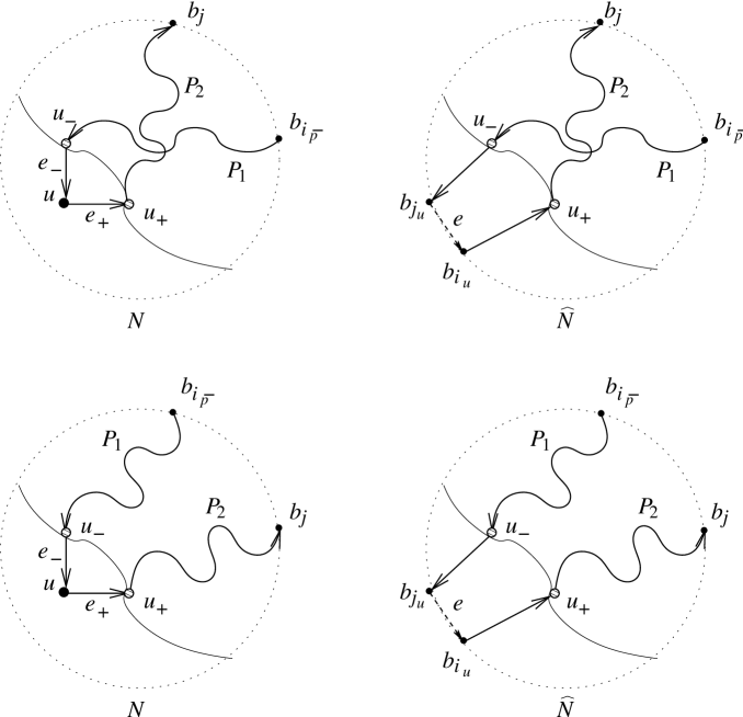
Figure 10. To the proof of Lemma 3.5

Assume first that

$$i_{\bar{p}}\prec j\preceq i_{p}-1\prec j_{u}\prec i_{u}\prec i_{p}+1,$$

which corresponds to the upper part of Figure 10. Then

$$c(C_{{\widehat{P}}_{1}})=c_{{\widehat{P}}_{1}}+c_{i_{u}}+c^{\prime},$$

where $c_{{\widehat{P}}_{1}}$ is the contribution of all vertices of ${\widehat{P}}_{1}$, including $b_{i_{\bar{p}}}$ and $b_{j_{u}}$, $c_{i_{u}}$ is the contribution of two consecutive edges of the convex hull of boundary vertices of ${\widehat{N}}$ calculated at $b_{i_{u}}$, and $c^{\prime}$ is the total contribution calculated at the vertices of the convex hull lying between $b_{i_{u}}$ and $b_{i_{\bar{p}}}$. Similarly,

$$c(C_{{\widehat{P}}_{2}})=c_{{\widehat{P}}_{2}}+c_{j_{u}}+c^{\prime\prime},$$

where $c_{{\widehat{P}}_{2}}$ is the contribution of all vertices of ${\widehat{P}}_{2}$, including $b_{i_{u}}$ and $b_{j}$, $c_{j_{u}}$ is the contribution of two consecutive edges of the convex hull of boundary vertices of ${\widehat{N}}$ calculated at $b_{j_{u}}$, and $c^{\prime\prime}$ is the total contribution calculated at the vertices of the convex hull lying between $b_{j}$ and $b_{j_{u}}$. Finally,

$$c(C_{{\widehat{P}}})=c_{{\widehat{P}}_{1}}+c_{{\widehat{P}}_{2}}+c^{\prime\prime}+c_{j_{u}}+c_{i_{u}}+c^{\prime},$$

and so $c(C_{{\widehat{P}}})=c(C_{{\widehat{P}}_{1}})+c(C_{{\widehat{P}}_{2}})$. Therefore, in this case $w_{P}=-w_{P_{1}}w_{e_{-}}w_{e_{+}}w_{P_{2}}$, and the contribution of all such paths to $M({i_{\bar{p}}},j)$ equals $-x^{\prime\prime}{\widehat{M}}({i_{\bar{p}}},{j_{u}}){\widehat{M}}({i_{u}},j)$. Each additional traversing of the edge $e_{+}$ results in multiplying this expression by $-x^{\prime\prime}{\widehat{M}}({i_{u}},{j_{u}})$; the proof of this fact is similar to the proof of Proposition 2.3. Summing up we get the second formula with the $-$ sign, as desired.

Assume now that

$$i_{p}-1\prec j_{u}\prec i_{u}\prec i_{p}+1\preceq j\prec i_{\bar{p}},$$

which corresponds to the lower part of Figure 10. Then

$$c(C_{{\widehat{P}}_{1}})=c_{{\widehat{P}}_{1}}+c_{i_{u}}+c^{\prime}+c_{j}+c^{\prime\prime\prime},$$

where $c_{{\widehat{P}}_{1}}$ and $c_{i_{u}}$ are as in the previous case, $c_{j}$ is the contribution of two consecutive edges of the convex hull of boundary vertices of ${\widehat{N}}$ calculated at $b_{j}$, $c^{\prime}$ is the total contribution calculated at the vertices of the convex hull lying between $b_{i_{u}}$ and $b_{j}$, and $c^{\prime\prime\prime}$ is the total contribution calculated at the vertices of the convex hull lying between $b_{j}$ and $b_{i_{\bar{p}}}$. Similarly,

$$c(C_{{\widehat{P}}_{2}})=c_{{\widehat{P}}_{2}}+c^{\prime\prime\prime}+c_{i_{\bar{p}}}+c^{\prime\prime}+c_{j_{u}},$$

where $c_{{\widehat{P}}_{2}}$ and $c_{j_{u}}$ are as in the previous case, $c_{i_{\bar{p}}}$ is the contribution of two consecutive edges of the convex hull of boundary vertices of ${\widehat{N}}$ calculated at $b_{i_{\bar{p}}}$, and $c^{\prime\prime}$ is the total contribution calculated at the vertices of the convex hull lying between $b_{i_{\bar{p}}}$ and $b_{j_{u}}$. Finally, $c(C_{{\widehat{P}}})=c_{{\widehat{P}}_{1}}+c_{{\widehat{P}}_{2}}+c^{\prime\prime\prime}$, and so $c(C_{{\widehat{P}}})=c(C_{{\widehat{P}}_{1}})+c(C_{{\widehat{P}}_{2}})+1$, since

$$c^{\prime}+c^{\prime\prime}+c^{\prime\prime\prime}+c_{j_{u}}+c_{i_{u}}+c_{j}+c_{i_{\bar{p}}}=0.$$

Therefore, in this case $w_{P}=w_{P_{1}}w_{e_{-}}w_{e_{+}}w_{P_{2}}$, and the contribution of all such paths to $M({i_{\bar{p}}},j)$ equals $x^{\prime\prime}{\widehat{M}}({i_{\bar{p}}},{j_{u}}){\widehat{M}}({i_{u}},j)$. Each additional traversing of $e_{+}$ once again results in multiplying this expression by $-x^{\prime\prime}{\widehat{M}}({i_{u}},{j_{u}})$. Summing up we get the second formula with the $+$ sign, as desired.

To treat the remaining two cases one makes use of Remark 2.2 and applies the same reasoning. ∎

Since ${\widehat{N}}$ has $r-1$ inner vertices, ${\widehat{M}}(i,j)$ satisfy relations similar to (3.20) with $N$ replaced by ${\widehat{N}}$, $I$ replaced by $I\setminus i_{p}\cup i_{v}$ and $J$ replaced by $J\cup j_{v}$. Relations (3.20) follow from this fact and Lemma 3.5 via simple though tedious computations.

For example, let $i_{\bar{p}}\prec j_{\bar{q}}\preceq i_{p}-1\prec j_{u}\prec i_{u}\prec i_{p}+1$. Then the left hand side of (3.20) is given by

$$\{M_{pq},M_{p\bar{q}}\}_{N} =\left\{\frac{x^{\prime}{\widehat{M}}({i_{u}},j_{q})}{1+x^{\prime\prime}{\widehat{M}}({i_{u}},{j_{u}})},{\widehat{M}}({i_{\bar{p}}},j_{\bar{q}})-\frac{x^{\prime\prime}{\widehat{M}}({i_{\bar{p}}},{j_{u}}){\widehat{M}}({i_{u}},j_{\bar{q}})}{1+x^{\prime\prime}{\widehat{M}}({i_{u}},{j_{u}})}\right\}_{N}$$

$$=\frac{x^{\prime}}{1+x^{\prime\prime}{\widehat{M}}({i_{u}},{j_{u}})}\{{\widehat{M}}(i_{u},j_{q}),{\widehat{M}}(i_{\bar{p}},j_{\bar{q}})\}_{\widehat{N}}$$

$$-\frac{x^{\prime}x^{\prime\prime}{\widehat{M}}(i_{u},j_{q})}{(1+x^{\prime\prime}{\widehat{M}}({i_{u}},{j_{u}}))^{2}}\{{\widehat{M}}(i_{u},j_{u}),{\widehat{M}}(i_{\bar{p}},j_{\bar{q}})\}_{\widehat{N}}$$

$$-\frac{{\widehat{M}}({i_{u}},j_{q}){\widehat{M}}({i_{\bar{p}}},j_{u}){\widehat{M}}(i_{u},j_{\bar{q}})}{(1+x^{\prime\prime}{\widehat{M}}({i_{u}},{j_{u}}))^{2}}\{x^{\prime},x^{\prime\prime}\}_{u}$$

$$-\frac{x^{\prime}x^{\prime\prime}{\widehat{M}}(i_{u},j_{\bar{q}})}{(1+x^{\prime\prime}{\widehat{M}}({i_{u}},{j_{u}}))^{2}}\{{\widehat{M}}(i_{u},j_{q}),{\widehat{M}}(i_{\bar{p}},j_{u})\}_{\widehat{N}}$$

$$-\frac{x^{\prime}x^{\prime\prime}{\widehat{M}}(i_{\bar{p}},j_{u})}{(1+x^{\prime\prime}{\widehat{M}}({i_{u}},{j_{u}}))^{2}}\{{\widehat{M}}(i_{u},j_{q}),{\widehat{M}}(i_{u},j_{\bar{q}})\}_{\widehat{N}}$$

$$+\frac{x^{\prime}(x^{\prime\prime})^{2}{\widehat{M}}(i_{u},j_{\bar{q}}){\widehat{M}}(i_{u},j_{q})}{(1+x^{\prime\prime}{\widehat{M}}({i_{u}},{j_{u}}))^{3}}\{{\widehat{M}}(i_{u},j_{u}),{\widehat{M}}(i_{\bar{p}},j_{u})\}_{\widehat{N}}$$

$$+\frac{x^{\prime}(x^{\prime\prime})^{2}{\widehat{M}}(i_{u},j_{q}){\widehat{M}}(i_{\bar{p}},j_{u})}{(1+x^{\prime\prime}{\widehat{M}}({i_{u}},{j_{u}}))^{3}}\{{\widehat{M}}(i_{u},j_{u}),{\widehat{M}}(i_{u},j_{\bar{q}})\}_{\widehat{N}}$$

$$+\frac{x^{\prime}(x^{\prime\prime})^{2}{\widehat{M}}(i_{\bar{p}},j_{u}){\widehat{M}}(i_{u},j_{\bar{q}})}{(1+x^{\prime\prime}{\widehat{M}}({i_{u}},{j_{u}}))^{3}}\{{\widehat{M}}(i_{u},j_{q}),{\widehat{M}}(i_{u},j_{u})\}_{\widehat{N}}$$

$$+\frac{x^{\prime\prime}{\widehat{M}}(i_{\bar{p}},j_{u}){\widehat{M}}(i_{u},j_{\bar{q}}){\widehat{M}}(i_{u},j_{q}),{\widehat{M}}(i_{u},j_{u})}{(1+x^{\prime\prime}{\widehat{M}}({i_{u}},{j_{u}}))^{3}}\{x^{\prime},x^{\prime\prime}\}_{u},$$

and the right hand side is given by

$$( \alpha-\beta)s_{=}(i_{p},j_{q},i_{\bar{p}},j_{\bar{q}})\frac{x^{\prime}{\widehat{M}}({i_{u}},j_{\bar{q}})}{1+x^{\prime\prime}{\widehat{M}}({i_{u}},{j_{u}})}\left({\widehat{M}}({i_{\bar{p}}},j_{q})-\frac{x^{\prime\prime}{\widehat{M}}({i_{\bar{p}}},{j_{u}}){\widehat{M}}({i_{u}},j_{q})}{1+x^{\prime\prime}{\widehat{M}}({i_{u}},{j_{u}})}\right)$$

$$+(\alpha+\beta)s_{\times}(i_{p},j_{q},i_{\bar{p}},j_{\bar{q}})\frac{x^{\prime}{\widehat{M}}({i_{u}},j_{q})}{1+x^{\prime\prime}{\widehat{M}}({i_{u}},{j_{u}})}\left({\widehat{M}}({i_{\bar{p}}},j_{\bar{q}})-\frac{x^{\prime\prime}{\widehat{M}}({i_{\bar{p}}},{j_{u}}){\widehat{M}}({i_{u}},j_{\bar{q}})}{1+x^{\prime\prime}{\widehat{M}}({i_{u}},{j_{u}})}\right).$$

Treating ${\widehat{M}}(\cdot,\cdot)$, $\alpha-\beta$ and $\alpha+\beta$ as independent variables and equating coefficients of the same monomials in the above two expressions we arrive to the following identities:

$$s_{=}(i_{u},j_{q},i_{\bar{p}},j_{\bar{q}})=s_{=}(i_{p},j_{q},i_{\bar{p}},j_{\bar{q}}),\qquad s_{\times}(i_{u},j_{q},i_{\bar{p}},j_{\bar{q}})=s_{\times}(i_{p},j_{q},i_{\bar{p}},j_{\bar{q}}),$$

$$s_{=}(i_{u},j_{u},i_{\bar{p}},j_{\bar{q}})+s_{=}(i_{u},j_{q},i_{\bar{p}},j_{u})+s_{=}(i_{u},j_{q},i_{u},j_{\bar{q}})-1/2=s_{=}(i_{p},j_{q},i_{\bar{p}},j_{\bar{q}}),$$

$$s_{\times}(i_{u},j_{u},i_{\bar{p}},j_{\bar{q}})+s_{\times}(i_{u},j_{q},i_{\bar{p}},j_{u})+s_{\times}(i_{u},j_{q},i_{u},j_{\bar{q}})+1/2=s_{\times}(i_{p},j_{q},i_{\bar{p}},j_{\bar{q}}),$$

$$s_{=}(i_{u},j_{u},i_{\bar{p}},j_{u})+s_{=}(i_{u},j_{u},i_{u},j_{\bar{q}})+s_{=}(i_{u},j_{q},i_{u},j_{u})-1/2=0,$$

$$s_{\times}(i_{u},j_{u},i_{\bar{p}},j_{u})+s_{\times}(i_{u},j_{u},i_{u},j_{\bar{q}})+s_{\times}(i_{u},j_{q},i_{u},j_{u})+1/2=0.$$

The latter can be checked easily by considering separately the following cases: $i_{p}\prec j_{q}\prec i_{\bar{p}}$; $i_{\bar{p}}\prec j_{q}\prec j_{\bar{q}}$; $j_{q}=j_{\bar{q}}$; $j_{\bar{q}}\prec j_{q}\prec i_{p}$. In each one of these cases all the functions involved in the above identities take constant values. ∎

4. Grassmannian boundary measurement map and induced Poisson structures on $G_{k}(n)$

4.1. Plücker coordinates and Poisson brackets

Let us recall the construction of Poisson brackets on the Grassmannian from [GSV1]. Let $G_{k}(n)$ be the Grassmannian of $k$-dimensional subspaces in ${\mathbb{R}}^{n}$. Given a $k$-element subset $I$ of $[1,n]=\{1,\dots,n\}$, the Plücker coordinate $x_{I}$ is a function on the set of $k\times n$ matrices which is equal to the value of the minor formed by the columns of the matrix indexed by the elements of $I$. In what follows, we use notation

$$I(i_{\alpha}\to l)=\{i_{1},\ldots,i_{\alpha-1},l,i_{\alpha+1},\ldots,i_{k}\}$$

for $\alpha\in[1,k]$ and $l\in[1,n]$.

Let $G^{0}_{k}(n)$ be the open cell in $G_{k}(n)$ characterized by non-vanishing of the Plücker coordinate $x_{[1,k]}$. Elements of $G^{0}_{k}(n)$ are parametrized by $k\times(n-k)$ matrices in the following way: if $W\in SL_{n}$ admits a factorization into block-triangular matrices

$$W=\begin{pmatrix}W_{11}&0\\ W_{12}&W_{22}\end{pmatrix}\begin{pmatrix}\mathbf{1}_{k}&Y\\ 0&\mathbf{1}_{n-k}\end{pmatrix},$$ (4.1)

then $Y=Y(W)$ represents an element of the cell $G^{0}_{k}(n)$.

It is easy to check that Plücker coordinates $x_{I}$, $I=\{i_{1},\ldots,i_{k}\ :1\leq i_{1}<\cdots<i_{k}\leq n\}$ of an element of $G^{0}_{k}(n)$ represented by $[\mathbf{1}_{k}\ Y]$ and minors $Y_{\alpha_{1},\ldots,\alpha_{l}}^{\beta_{1},\ldots,\beta_{l}}=\det(y_{\alpha_{i},\beta_{j}})_{i,j=1}^{l}$ of $Y$ are related via

$$Y_{\alpha_{1},\ldots,\alpha_{l}}^{\beta_{1},\ldots,\beta_{l}}=(-1)^{kl-l(l-1)/2-(\alpha_{1}+\cdots+\alpha_{l})}\frac{x_{([1,k]\setminus\{\alpha_{1},\ldots,\alpha_{l}\})\cup\{\beta_{1}+k,\ldots,\beta_{l}+k\}}}{x_{[1,k]}}.$$

Note that, if the row index set $\{\alpha_{1},\ldots,\alpha_{l}\}$ in the above formula is contiguous then the sign in the right hand side can be expressed as $(-1)^{(k-\alpha_{l})l}$.

A Poisson bracket ${\{\cdot,\cdot\}}$ on $G^{0}_{k}(n)$ is defined via the relation

$$\{f_{1}\circ Y,f_{2}\circ Y\}_{\operatorname{Mat}_{n}}=\{f_{1},f_{2}\}\circ Y\ .$$

In terms of matrix elements $y_{ij}$ of $Y$, this bracket looks as follows:

$$2\{y_{ij},y_{\alpha\beta}\}=(\operatorname{sign}(\alpha-i)-\operatorname{sign}(\beta-j))y_{i\beta}y_{\alpha j}.$$ (4.2)

4.2. Recovering the Sklyanin bracket on $\operatorname{Mat}_{k}$

Let us take a closer look at the 2-parameter family of Poisson brackets obtained in Theorem 3.3 in the case when vertices $b_{1},\dots,b_{k}$ on the boundary of the disk are sources and vertices $b_{k+1},\dots,b_{n}$ are sinks, that is, when $I=[1,k]$ and $J=[k+1,n]$. To simplify notation, in this situation we will write $\{\cdot,\cdot\}_{k,m}$ and $\operatorname{Net}_{k,m}$ instead of $\{\cdot,\cdot\}_{[1,k],[k+1,n]}$ and $\operatorname{Net}_{[1,k],[k+1,n]}$. Therefore, formula (3.16) can be re-written as

$$2\{M_{ij},M_{\bar{\imath}\bar{\jmath}}\}_{k,m}=(\alpha-\beta)\left(\operatorname{sign}(\bar{\imath}-i)-\operatorname{sign}(\bar{\jmath}-j)\right)M_{i\bar{\jmath}}M_{\bar{\imath}j}\\ +(\alpha+\beta)\left(\operatorname{sign}(\bar{\imath}-i)+\operatorname{sign}(\bar{\jmath}-j)\right)M_{ij}M_{\bar{\imath}\bar{\jmath}},$$ (4.3)

where $M_{ij}$ corresponds to the boundary measurement between $b_{i}$ and $b_{j+k}$. The first term in the equation above coincides (up to a multiple) with (4.2). This suggests that it makes sense to investigate Poisson properties of the boundary measurement map viewed as a map into $G_{k}(n)$, which will be the goal of this section.

First, however, we will go back to the example, considered in Sect. 3.1, where we associated with a network $N\in\operatorname{Net}_{k,k}$ a matrix $A_{N}=M_{N}W_{0}\in\operatorname{Mat}_{k}$. Written in terms of matrix entries $A_{ij}$ of $A$, bracket (4.3) becomes

$$2\{A_{ij},A_{\bar{\imath}\bar{\jmath}}\}_{k,m}=(\alpha-\beta)\left(\operatorname{sign}(\bar{\imath}-i)+\operatorname{sign}(\bar{\jmath}-j)\right)A_{i\bar{\jmath}}A_{\bar{\imath}j}\\ +(\alpha+\beta)\left(\operatorname{sign}(\bar{\imath}-i)-\operatorname{sign}(\bar{\jmath}-j)\right)A_{ij}A_{\bar{\imath}\bar{\jmath}}.$$ (4.4)

If $A_{N_{1}},A_{N_{2}}$ are matrices that correspond to networks $N_{1},N_{2}\in\operatorname{Net}_{k,k}$ then their product $A_{N_{1}}A_{N_{2}}$ corresponds to the concatenation of $N_{1}$ and $N_{2}$. This fact combined with Theorem 3.2 implies that the bracket (4.4) possesses the Poisson-Lie property.

In fact, (4.4) is the Sklyanin bracket  (3.3) on $\operatorname{Mat}_{k}$ associated with a deformation of the standard R-matrix (3.4). Indeed, it is known (see [ReST]) that if $R_{0}$ is the standard R-matrix, $S$ is any linear operator on the set of diagonal matrices that is skew-symmetric w.r.t. the trace-form, and $\pi_{0}$ is the natural projection onto a subspace of diagonal matrices, then for any scalar $c_{1}$, $c_{2}$ the linear combination $c_{1}R_{0}+c_{2}S\pi_{0}$ satisfies MCYBE (3.1) and thus gives rise to a Sklyanin Poisson-Lie bracket.

Define $S$ by

$$S(e_{jj})=\sum_{i=1}^{k}\operatorname{sign}(j-i)e_{ii},\quad j=1,\ldots,k,$$

and put

$$R_{\alpha,\beta}=\frac{\alpha-\beta}{2}R_{0}+\frac{\alpha+\beta}{2}S\pi_{0}.$$

Substituting coordinate functions $A_{ij}$, $A_{i^{\prime}j^{\prime}}$ into expression (3.3) for the Sklyanin Poisson-Lie bracket associated with the R-matrix $R_{\alpha,\beta}$, we recover equation (4.4).

To summarize, we obtained

Theorem 4.1.

For any network $N\in\operatorname{Net}_{k,k}$ and any choice of parameters $\alpha_{ij}$, $\beta_{ij}$ in (3.7), (3.8), the map $A_{N}:{({\mathbb{R}}\setminus 0)}^{|E|}\to\operatorname{Mat}_{k}$ is Poisson with respect to the Sklyanin bracket  (3.3) associated with the R-matrix $R_{\alpha,\beta}$, where $\alpha$ and $\beta$ satisfy relations (3.11) and (3.13).

4.3. Induced Poisson structures on $G_{k}(n)$

Let $N$ be a network with the sources $b_{i}$, $i\in I$ and sinks $b_{j}$, $j\in J$. Following [P], we are going to interpret the boundary measurement map as a map into the Grassmannian $G_{k}(n)$. To this end, we extend $M_{N}$ to a $k\times n$ matrix ${\bar{X}}_{N}$ as follows:

(i) the $k\times k$ submatrix of ${\bar{X}}_{N}$ formed by $k$ columns indexed by $I$ is the identity matrix $\mathbf{1}_{k}$;

(ii) for $p\in[1,k]$ and $j=j_{q}\in J$, the $(p,j)$-entry of ${\bar{X}}_{N}$ is

$$m^{I}_{pj}=(-1)^{s(p,j)}M_{pq},$$

where $s(p,j)$ is the number of elements in $I$ lying strictly between $\min\{i_{p},j\}$ and $\max\{i_{p},j\}$ in the linear ordering; note that the sign is selected in such a way that the minor $({\bar{X}}_{N})_{[1,k]}^{I(i_{p}\to j)}$ coincides with $M_{pq}$.

We will view ${\bar{X}}_{N}$ as a matrix representative of an element $X_{N}\in G_{k}(n)$. The corresponding rational map $X_{N}{:\ }{\mathcal{E}}_{N}\to G_{k}(n)$ is called the Grassmannian boundary measurement map. For example, the network presented in Figure 11 defines a map of ${({\mathbb{R}}\setminus 0)}^{8}$ to $G_{2}(4)$ given by the matrix

$$\begin{pmatrix}&1&\dfrac{w_{1}w_{4}w_{6}}{1+w_{2}w_{4}w_{5}w_{7}}&0&-\dfrac{w_{1}w_{3}w_{4}w_{5}w_{7}}{1+w_{2}w_{4}w_{5}w_{7}}\\ \\ &0&\dfrac{w_{2}w_{4}w_{5}w_{6}w_{8}}{1+w_{2}w_{4}w_{5}w_{7}}&1&\dfrac{w_{3}w_{5}w_{8}}{1+w_{2}w_{4}w_{5}w_{7}}\end{pmatrix}.$$

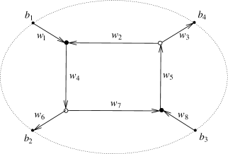
Figure 11. To the definition of the Grassmannian boundary measurement map

Clearly, $X_{N}$ belongs to the cell $G_{k}^{I}(n)=\{X\in G_{k}(n)\ :\ x_{I}\neq 0\}$. Therefore, we can regard matrix entries $m^{I}_{pj}$ as coordinate functions on $G_{k}^{I}(n)$ and rewrite (3.16) as follows:

$$\{m^{I}_{pj},m^{I}_{\bar{p}\bar{\jmath}}\}_{I,J}=(\alpha-\beta)s_{=}(i_{p},j,i_{\bar{p}},\bar{\jmath})m^{I}_{p\bar{\jmath}}m^{I}_{\bar{p}j}+(\alpha+\beta)s_{\times}(i_{p},j,i_{\bar{p}},\bar{\jmath})m^{I}_{pj}m^{I}_{\bar{p}\bar{\jmath}}.$$ (4.5)

Remark 4.2.

If $I=[1,k]$, then the 2-parametric family (4.5) of Poisson brackets on $G_{k}^{I}(n)=G_{k}^{0}(n)$ is defined by (4.3). A computation identical to the one presented in [GSV1] (see Sect. 4.1) shows that (4.3) is the pushforward to $G_{k}^{0}(n)$ of the Sklyanin Poisson-Lie bracket (3.3) on $\operatorname{Mat}_{n}$ associated with the R-matrix $R_{\alpha,\beta}$.

The following result says that the families $\{\cdot,\cdot\}_{I,J}$ on different cells $G^{I}_{k}(n)$ can be glued together to form the unique 2-parametric family of Poisson brackets on $G_{k}(n)$ that makes all maps $X_{N}$ Poisson.

Theorem 4.3.

(i) For any choice of parameters $\alpha$ and $\beta$ there exists a unique Poisson bracket ${\mathcal{P}}_{\alpha,\beta}$ on $G_{k}(n)$ such that for any network $N$ with $k$ sources, $n-k$ sinks and weights defined by (3.6), the map $X_{N}{:\ }{({\mathbb{R}}\setminus 0)}^{|E|}\to G_{k}(n)$ is Poisson provided the parameters $\alpha_{ij}$ and $\beta_{ij}$ defining the bracket $\{\cdot,\cdot\}_{N}$ on ${({\mathbb{R}}\setminus 0)}^{|E|}$ satisfy relations (3.11) and (3.13).

(ii) For any $I\subset[1,n]$, $|I|=k$, and $J=[1,n]\setminus I$, the restriction of ${\mathcal{P}}_{\alpha,\beta}$ to the cell $G^{I}_{k}(n)$ coincides with the bracket $\{\cdot,\cdot\}_{I,J}$ given by (4.5) in coordinates $m^{I}_{pj}$.

Proof.

Both statements follow immediately from Theorems 3.2 and 3.3, the fact that $G_{k}^{0}(n)$ is an open dense subset in $G_{k}(n)$, and the following proposition.

Proposition 4.4.

For any $i_{p},i_{\bar{p}}\in I$ and any $j,\bar{\jmath}\in J$,

$$\{m^{I}_{pj},m^{I}_{{\bar{p}}\bar{\jmath}}\}_{k,n-k}=\{m^{I}_{pj},m^{I}_{{\bar{p}}\bar{\jmath}}\}_{I,J}.$$ (4.6)

Proof.

It is convenient to rewrite (4.5) as

$$\{m^{I}_{pj},m^{I}_{\bar{p}\bar{\jmath}}\}_{I,J}=\{m^{I}_{pj},m^{I}_{\bar{p}\bar{\jmath}}\}^{1}_{I,J}+\{m^{I}_{pj},m^{I}_{\bar{p}\bar{\jmath}}\}^{2}_{I,J}$$

and to treat the brackets $\{\cdot,\cdot\}^{1}_{I,J}$ and $\{\cdot,\cdot\}^{2}_{I,J}$ separately for a suitable choice of parameters $\alpha$ and $\beta$.

Let $I=[1,k]$ and denote $m_{ij}^{[1,k]}$ simply by $m_{ij}$. Then two independent brackets are given by

$$\{m_{ij},m_{\bar{\imath}\bar{\jmath}}\}^{1}_{k,n-k}=\left(\operatorname{sign}(\bar{\imath}-i)-\operatorname{sign}(\bar{\jmath}-j)\right)m_{i\bar{\jmath}}m_{\bar{\imath}j}.$$ (4.7)

(for $\alpha-\beta=2$) that coincides (up to a multiple) with the Poisson bracket (4.2) on $G^{0}_{k}(n)$ and

$$\{m_{ij},m_{\bar{\imath}\bar{\jmath}}\}^{2}_{k,n-k}=\left(\operatorname{sign}(\bar{\imath}-i)+\operatorname{sign}(\bar{\jmath}-j)\right)m_{ij}m_{\bar{\imath}\bar{\jmath}}$$ (4.8)

(for $\alpha+\beta=2$).

Let us start with the first of the two brackets above. For a generic element $X$ in $G_{k}(n)$ represented by a matrix ${\bar{X}}={\bar{X}}_{N}$, consider any two minors, ${\bar{X}}_{\mu}^{\nu}$ and ${\bar{X}}_{\mu^{\prime}}^{\nu^{\prime}}$, with row sets $\mu=(\mu_{1},\ldots,\mu_{l})$, $\mu^{\prime}=(\mu^{\prime}_{1},\ldots,\mu^{\prime}_{l^{\prime}})$, $\mu,\mu^{\prime}\subseteq[1,k]$ and column sets $\nu=(\nu_{1},\ldots,\nu_{l})$, $\nu^{\prime}=(\nu^{\prime}_{1},\ldots,\nu^{\prime}_{l^{\prime}})$, $\nu,\nu^{\prime}\subseteq[k+1,n]$. Using considerations similar to those in the proof of Lemma 3.2 in [GSV1], we obtain from (4.7)

$$\{{\bar{X}}_{\mu}^{\nu},{\bar{X}}_{\mu^{\prime}}^{\nu^{\prime}}\}^{1}_{k,n-k}=\sum_{p=1}^{l}\sum_{q=1}^{l^{\prime}}\left(\operatorname{sign}(\mu^{\prime}_{p}-\mu_{q}){\bar{X}}_{\mu(\mu_{p}\to\mu^{\prime}_{q})}^{\nu}{\bar{X}}_{\mu^{\prime}(\mu^{\prime}_{q}\to\mu_{p})}^{\nu^{\prime}}\right.\\ -\left.\operatorname{sign}(\nu^{\prime}_{p}-\nu_{q}){\bar{X}}_{\mu}^{\nu(\nu_{p}\to\nu^{\prime}_{q})}{\bar{X}}_{\mu^{\prime}}^{\nu^{\prime}(\nu^{\prime}_{q}\to\nu_{p})}\right).$$ (4.9)

Plücker coordinates $x_{I}$ (for $I\subset[1,n]$, $|I|=k$) and minors ${\bar{X}}_{\mu}^{\nu}$ are related via

$${\bar{X}}_{\mu}^{\nu}=(-1)^{l(l-1)/2}\frac{x_{([1,k]\setminus\mu)\cup\{\nu\}}}{x_{[1,k]}}.$$

Denote

$$a_{I}=\frac{x_{I}}{x_{[1,k]}}=(-1)^{l(l-1)/2}{\bar{X}}_{[1,k]\setminus I}^{I\setminus[1,k]},$$

where $l=\left|[1,k]\setminus I\right|$. Then (4.9) gives rise to Poisson relations

$$\{a_{I},a_{I^{\prime}}\}^{1}_{k,n-k} =\sum_{i\in I\cap[1,k]}\sum_{i^{\prime}\in I^{\prime}\cap[1,k]}\operatorname{sign}(i-i^{\prime})a_{I(i\to i^{\prime})}a_{I^{\prime}(i^{\prime}\to i)}$$

$$+\sum_{i\in I\setminus[1,k]}\sum_{i^{\prime}\in I^{\prime}\setminus[1,k]}\operatorname{sign}(i-i^{\prime})a_{I(i\to i^{\prime})}a_{I^{\prime}(i^{\prime}\to i)}$$

$$=\sum_{i\in I}\sum_{i^{\prime}\in I^{\prime}}\varepsilon_{ii^{\prime}}a_{I(i\to i^{\prime})}a_{I^{\prime}(i^{\prime}\to i)},$$

where

$$\varepsilon_{ii^{\prime}}=\left\{\begin{array}[]{cc}0&\mbox{if}\quad i\leq k<\bar{\imath}\quad\mbox{or}\quad\bar{\imath}\leq k<i,\\ \operatorname{sign}(i-i^{\prime})&\mbox{otherwise}.\end{array}\right.$$

Let us fix a $k$-element index set $I=\{1\leq i_{1}<\ldots<i_{k}\leq n\}$ and use (4.3) to compute, for any $p,\bar{p}\in[1,k]$ and $j,\bar{\jmath}\notin I$, the bracket $\{m_{pj}^{I},m_{\bar{p}\bar{\jmath}}^{I}\}^{1}_{k,n-k}$. Taking into account that

$$m^{I}_{pj}=\frac{x_{I(i_{p}\to j)}}{x_{I}}\quad\text{for any $p\in[1,k]$, $j\in J$},$$

we get

$$\{m^{I}_{pj},m^{I}_{{\bar{p}}\bar{\jmath}}\}^{1}_{k,n-k} =\dfrac{1}{a_{I}^{2}}\bigg{(}\{a_{I(i_{p}\to j)},a_{I(i_{\bar{p}}\to\bar{\jmath})}\}^{1}_{k,n-k}-\dfrac{a_{I(i_{p}\to j)}}{a_{I}}\{a_{I},a_{I(i_{\bar{p}}\to\bar{\jmath})}\}^{1}_{k,n-k}$$

$$\qquad\qquad\dfrac{a_{I(i_{\bar{p}}\to\bar{\jmath})}}{a_{I}}\{a_{I(i_{p}\to j)},a_{I}\}^{1}_{k,n-k}\bigg{)}$$

$$=\dfrac{1}{a_{I}^{2}}\big{(}(\varepsilon_{j\bar{\jmath}}+\varepsilon_{i_{\bar{p}}i_{p}})a_{I(i_{p}\to\bar{\jmath})}a_{I(i_{\bar{p}}\to j)}+(\varepsilon_{ji_{p}}+\varepsilon_{i_{\bar{p}}\bar{\jmath}})a_{I}a_{I(i_{p}\to j,i_{\bar{p}}\to\bar{\jmath})}$$

$$\qquad\qquad-(\varepsilon_{ji_{p}}+\varepsilon_{i_{\bar{p}}\bar{\jmath}})a_{I(i_{p}\to j)}a_{I(i_{\bar{p}}\to\bar{\jmath})}\big{)}$$

$$=\dfrac{1}{a_{I}^{2}}(\varepsilon_{j\bar{\jmath}}+\varepsilon_{i_{\bar{p}}i_{p}}-\varepsilon_{ji_{p}}-\varepsilon_{i_{\bar{p}}\bar{\jmath}})a_{I(i_{p}\to\bar{\jmath})}a_{I(i_{\bar{p}}\to j)}$$

$$=(\varepsilon_{j\bar{\jmath}}+\varepsilon_{i_{\bar{p}}i_{p}}-\varepsilon_{ji_{p}}-\varepsilon_{i_{\bar{p}}\bar{\jmath}})m^{I}_{p\bar{\jmath}}m^{I}_{{\bar{p}}j},$$

where in the third step we have used the short Plücker relation.

Relation (4.6) for the first bracket follows from

Lemma 4.5.

For any $i_{p},i_{\bar{p}}\in I$ and any $j,\bar{\jmath}\notin I$,

$$\varepsilon_{j\bar{\jmath}}+\varepsilon_{i_{\bar{p}}i_{p}}-\varepsilon_{ji_{p}}-\varepsilon_{i_{\bar{p}}\bar{\jmath}}=2s_{=}(i_{p},j,i_{\bar{p}},\bar{\jmath}).$$ (4.10)

Proof.

Denote the left hand side of (4.10) by $\varepsilon^{1}(i_{p},j,\bar{\jmath},i_{\bar{p}})$. Let us prove that this expression depends only on the counterclockwise order of the numbers $i_{p}$, $j$, $\bar{\jmath}$, $i_{\bar{p}}$ and does not depend on the numbers themselves.

Assume first that all four numbers are distinct. In this case $\varepsilon^{1}(i_{p},j,\bar{\jmath},i_{\bar{p}})$ is invariant with respect to the cyclic shift of the variables, hence it suffices to verify the identity $\varepsilon^{1}(i_{p},j,\bar{\jmath},i_{\bar{p}})=\varepsilon^{1}(i_{p},j-1\mod n,\bar{\jmath},i_{\bar{p}})$ provided the counterclockwise orders of $i_{p}$, $j$, $\bar{\jmath}$, $i_{\bar{p}}$ and $i_{p}$, $j-1\mod n$, $\bar{\jmath}$, $i_{\bar{p}}$ coincide. This is trivial unless $j=1$ or $j=k$, since all four summands retain their values. In the remaining cases the second and the fourth summands retain their values, and we have to check the identities $\varepsilon_{1\bar{\jmath}}-\varepsilon_{1i_{p}}=\varepsilon_{n\bar{\jmath}}-\varepsilon_{ni_{p}}$ and $\varepsilon_{k\bar{\jmath}}-\varepsilon_{ki_{p}}=\varepsilon_{k-1,\bar{\jmath}}-\varepsilon_{k-1,i_{p}}$. The first of them follows from the identity $\varepsilon_{ni}=\varepsilon_{1i}+1$ for $i\neq 1,n$, and the second one, from the identity $\varepsilon_{k-1,i}=\varepsilon_{ki}+1$ for $i\neq k-1,k$.

If $j=\bar{\jmath}$ or $i_{p}=i_{\bar{p}}$ (other coincidences are impossible since $i_{p},i_{\bar{p}}\in I$, $j,\bar{\jmath}\notin I$), $\varepsilon^{1}$ degenerates to a function of three variables, which is again invariant with respect to cyclic shifts, therefore all the above argument applies as well.

To obtain (4.10) it remains to check that $\varepsilon^{1}(i_{p},1,k,i_{\bar{p}})=2s_{=}(i_{p},1,i_{\bar{p}},k)$, which can be done separately in all the cases mentioned in (3.14). ∎

Next, let us turn to the Poisson bracket (4.8). For any two monomials in matrix entries of ${\bar{X}}_{N}$, $\mathbf{x}=\prod_{p=1}^{l}{\bar{X}}_{\mu_{p}\nu_{p}}$, and $\mathbf{x}^{\prime}=\prod_{q=1}^{l^{\prime}}{\bar{X}}_{\mu^{\prime}_{q}\nu^{\prime}_{q}}$, we have

$$\{\mathbf{x},\mathbf{x}^{\prime}\}^{2}_{k,n-k}=\mathbf{x}\ \mathbf{x}^{\prime}\sum_{p=1}^{l}\sum_{q=1}^{l^{\prime}}\left(\operatorname{sign}(\mu^{\prime}_{p}-\mu_{q})+\operatorname{sign}(\nu^{\prime}_{p}-\nu_{q})\right).$$

Observe that the double sum above is invariant under any permutation of indices within sets $\mu=(\mu_{1},\ldots,\mu_{l})$, $\mu^{\prime}=(\mu^{\prime}_{1},\ldots,\mu^{\prime}_{l^{\prime}})$, $\nu=(\nu_{1},\ldots,\nu_{l})$, $\nu^{\prime}=(\nu^{\prime}_{1},\ldots,\nu^{\prime}_{l^{\prime}})$. This means that for minors ${\bar{X}}_{\mu}^{\nu},{\bar{X}}_{\mu^{\prime}}^{\nu^{\prime}}$ we have

$$\{{\bar{X}}_{\mu}^{\nu},{\bar{X}}_{\mu^{\prime}}^{\nu^{\prime}}\}^{2}_{k,n-k}={\bar{X}}_{\mu}^{\nu}{\bar{X}}_{\mu^{\prime}}^{\nu^{\prime}}\sum_{p=1}^{l}\sum_{q=1}^{l^{\prime}}\left(\operatorname{sign}(\mu^{\prime}_{p}-\mu_{q})+\operatorname{sign}(\nu^{\prime}_{p}-\nu_{q})\right),$$

and the resulting Poisson relations for functions $a_{I}$ are

$$\{a_{I},a_{I^{\prime}}\}^{2}_{k,n-k} =a_{I}a_{I^{\prime}}\left(\sum_{i\in[1,k]\setminus I}\sum_{i^{\prime}\in[1,k]\setminus I^{\prime}}\operatorname{sign}(i-i^{\prime})\right.$$

$$\qquad\qquad\qquad+\left.\sum_{i\in I\setminus[1,k]}\sum_{i^{\prime}\in I^{\prime}\setminus[1,k]}\operatorname{sign}(i-i^{\prime})\right)$$

$$=a_{I}a_{I^{\prime}}\sum_{i\in I}\sum_{i^{\prime}\in I^{\prime}}\varepsilon_{ii^{\prime}},$$

where $\varepsilon_{ii^{\prime}}$ has the same meaning as above. These relations imply

$$\{m^{I}_{i_{p}j},m^{I}_{i_{\bar{p}}\bar{\jmath}}\}^{2}_{k,n-k}=m^{I}_{i_{p}j}m^{I}_{i_{\bar{p}}\bar{\jmath}}\left(\varepsilon_{i_{p}i_{\bar{p}}}-\varepsilon_{i_{p}\bar{\jmath}}-\varepsilon_{qi_{\bar{p}}}+\varepsilon_{j\bar{\jmath}}\right).$$

Relation (4.6) for the second bracket follows now from

Lemma 4.6.

For any $i_{p},i_{\bar{p}}\in I$ and any $j,\bar{\jmath}\notin I$,

$$\varepsilon_{i_{p}i_{\bar{p}}}-\varepsilon_{i_{p}\bar{\jmath}}-\varepsilon_{qi_{\bar{p}}}+\varepsilon_{j\bar{\jmath}}=2s_{\times}(i_{p},j,i_{\bar{p}},\bar{\jmath}).$$ (4.11)

Proof.

The proof of (4.11) is similar to the proof of (4.10). ∎

This proves Proposition 4.4, and hence Theorem 4.3. ∎

∎

4.4. $GL_{n}$-action on the Grassmannian via networks

In this subsection we interpret the natural action of $GL_{n}$ on $G_{k}(n)$ in terms of planar networks.

First, note that any element of $GL_{n}$ can be represented by a planar network built by concatenation from building blocks (elementary networks) described in Fig. 5. To see this, one needs to observe that an elementary transposition matrix $S_{i}=\mathbf{1}-e_{ii}-e_{i+1,i+1}+e_{i,i+1}+e_{i+1,i}$ can be factored as

$$S_{i}=(\mathbf{1}-2e_{i+1,i+1})E_{i+1}^{-}(-1)E_{i+1}^{+}(1)E_{i+1}^{-}(-1),$$

which implies that any permutation matrix can be represented via concatenation of elementary networks. Consequently, any elementary triangular matrices $\mathbf{1}+ue_{ij}$, $\mathbf{1}+le_{ji}$, $i<j$, can be factored as

$$\mathbf{1}+ue_{ij}=W_{ij}E_{i+1}^{+}(u)W^{-1}_{ij},\qquad\mathbf{1}+le_{ji}=W^{-1}_{ij}E_{i+1}^{-}(l)W_{ij},$$

where $W_{ij}$ is the permutation matrix that corresponds to the permutation

$$(1)\cdots(i)(i+1\ldots j)(j+1)\cdots(n).$$

The claim then follows from the Bruhat decomposition and constructions presented in Section 3.1.

Consider now a network $N\in\operatorname{Net}_{I,J}$ and a network $N(A)$ representing an element $A\in GL_{n}$ as explained above. We will concatenate $N$ and $N(A)$ according to the following rule: in $N(A)$ reverse directions of all horizontal paths $i\to i$ for $i\in I$, changing every edge weight $w$ involved to $w^{-1}$, and then glue the left boundary of $N(A)$ to the boundary of $N$ in such a way that boundary vertices with the same label are glued to each other. Denote the resulting net by $N\circ N(A)$. Let ${\bar{X}}_{N}$ and ${\bar{X}}_{N\circ N(A)}$ be the signed boundary measurement matrices constructed according to the recipe outlined at the beginning of Section 4.3.

Lemma 4.7.

Matrices ${\bar{X}}_{N\circ N(A)}$ and ${\bar{X}}_{N}A$ are representatives of the same element in $G_{k}(n)$.

Proof.

To check that ${\bar{X}}_{N\circ N(A)}$ coincides with the result of the natural action of $GL_{n}$ on $G_{k}(n)$ induced by the right multiplication, it suffices to consider the case when $A$ is a diagonal or an elementary bidiagonal matrix, that is when $N(A)$ is one of the elementary networks in Fig. 5. If $N(A)$ is the first diagram in Fig. 5, then the boundary measurements in $N^{\prime}=N\circ N(A)$ are given by $M^{\prime}(i,j)=d_{i}^{-1}M(i,j)d_{j}$, $i\in I,j\in J$, where $M(i,j)$ are the boundary measurements in $N$. This is clearly consistent with the natural $GL_{n}$ action.

Now let $A=E_{i}^{-}(l)$ (the case $A=E_{i}^{+}(u)$ can be treated similarly). Then

$$M^{\prime}(i_{p},j)=\begin{cases}M(i_{p},j)+\delta_{ii_{p}}lM(i_{p-1},j)&\hskip-71.13188pt\text{if $i,i-1\in I$}\\ M(i_{p},j)+\delta_{i-1,j}lM(i_{p},j+1)&\hskip-71.13188pt\text{if $i,i-1\in J$}\\ M(i_{p},j)+\delta_{ii_{p}}\delta_{i-1,j}l&\hskip-71.13188pt\text{if $i\in I$, $i-1\in J$}\\ \dfrac{M(i-1,j)}{1+lM(i-1,i)}(\delta_{i_{p},i-1}\pm(1-\delta_{i_{p},i-1})lM(i_{p},i))&\\ \hskip 28.45274pt+(1-\delta_{i_{p},i-1})M(i_{p},j)&\hskip-71.13188pt\text{if $i\in J$, $i-1\in I$}\end{cases}$$ (4.12)

(in the last line above we used Lemma 3.5).

Recall that for $j\in J$, an entry ${\bar{X}}_{pj}$ of ${\bar{X}}_{N}$ coincides with $M(i_{p},j)$ up to the sign $(-1)^{s(p,j)}$. By the construction in Section 4.3, if $i,i-1\in I$, then $(-1)^{s(p,j)}=-(-1)^{s(p-1,j)}$ for $p$ such that $i_{p}=i$ and for all $j\in J$. Then the first line of (4.12) shows that ${\bar{X}}_{N^{\prime}}=E_{p}^{-}(-l){\bar{X}}_{N}E_{i}^{-}(l)$, where the first elementary matrix is $k\times k$ and the second one is $n\times n$.

If $i,i-1\in J$, then $(-1)^{s(p,i-1)}=(-1)^{s(p,i)}$ for all $p\in[1,k]$, and the second line of (4.12) results in ${\bar{X}}_{N^{\prime}}={\bar{X}}_{N}E_{i}^{-}(l)$. The latter equality is also clearly valid for the case $i\in I$, $i-1\in J$.

Finally, if $i\in J$, $i-1\in I$, let $r\in[1,k]$ be the index such that $i-1=i_{r}$, and let ${\bar{X}}_{N}^{(i)}$ denote the $i$th column of ${\bar{X}}_{N}$. Then the $k\times k$ submatrix of ${\bar{X}}_{N}E_{i}^{-}(l)$ formed by the columns indexed by $I$ is $C=\mathbf{1}_{k}+l{\bar{X}}_{N}^{(i)}e_{r}^{T}$, where $e_{r}=(0,\dots,0,1,0,\dots,0)$ with the only nonzero element in the $r$th position. Therefore,

$$\tilde{X}=C^{-1}{\bar{X}}_{N}E_{i}^{-}(l)=\left(\mathbf{1}_{k}-\frac{1}{1+l{\bar{X}}_{ri}}l{\bar{X}}_{N}^{(i)}e_{r}^{T}\right){\bar{X}}_{N}E_{i}^{-}(l)$$

is the representative of $[{\bar{X}}_{N}E_{i}^{-}(l)]\in G_{k}(n)$ that has an identity matrix as its $k\times k$ submatrix formed by columns indexed by $I$. We need to show that $\tilde{X}={\bar{X}}_{N^{\prime}}$. First note that ${\bar{X}}_{ri}=M(i_{r},i)=M(i-1,i)$ and so, for all $j\in J$,

$$\tilde{X}_{rj}=\frac{{\bar{X}}_{rj}}{1+l{\bar{X}}_{ri}}=\frac{(-1)^{s(r,j)}M(i-1,j)}{1+lM(i-1,i)}=(-1)^{s(r,j)}M^{\prime}(i-1,j)=({\bar{X}}_{N^{\prime}})_{rj}.$$

If $p\neq r$, then

$$\tilde{X}_{pj}={\bar{X}}_{pj}-\frac{l{\bar{X}}_{rj}{\bar{X}}_{pi}}{1+l{\bar{X}}_{ri}}\\ =(-1)^{s(p,j)}\left(M(i_{p},j)-(-1)^{s(p,i)+s(r,j)-s(p,j)}\frac{lM(i_{p},i)M(i-1,j)}{1+lM(i-1,i)}\right).$$

Thus, to see that $\tilde{X}_{pj}=({\bar{X}}_{N^{\prime}})_{rj}$, it is enough to check that the sign assignment that was used in Lemma 3.5 is consistent with the formula

$$-(-1)^{s(p,i)+s(r,j)-s(p,j)}.$$

This can be done by direct inspection and is left to the reader as an exercise. ∎

Recall that if $\mathcal{H}$ is a Lie subgroup of a Poisson-Lie group ${\mathcal{G}}$, then a Poisson structure on the homogeneous space $\mathcal{H}\backslash{\mathcal{G}}$ is called Poisson homogeneous if the action map $\mathcal{H}\backslash{\mathcal{G}}\times{\mathcal{G}}\to\mathcal{H}\backslash{\mathcal{G}}$ is Poisson. Now that we have established that the natural right action of $GL_{n}$ on $G_{k}(n)$ can be realized via the operation on networks described above, Theorems 3.3, 4.1 and 4.3 immediately imply the following

Theorem 4.8.

For any choice of parameters $\alpha,\beta$, the Grassmannian $G_{k}(n)$ equipped with the bracket ${\mathcal{P}}_{\alpha,\beta}$ is a Poisson homogeneous space for $GL_{n}$ equipped with the ”matching” Poisson-Lie bracket (4.4).

Remark 4.9.

It is not difficult to deduce Theorem 4.8 from the general theory of Poisson homogeneous spaces (see, e.g. [ReST]). The proof above illustrates capabilities of the network approach.

5. Compatibility with cluster algebra structure

5.1. Cluster algebras and compatible Poisson brackets

First, we recall the basics of cluster algebras of geometric type. The definition that we present below is not the most general one, see, e.g., [FZ3, BFZ2] for a detailed exposition.

The coefficient group ${\mathfrak{P}}$ is a free multiplicative abelian group of a finite rank $m$ with generators $g_{1},\dots,g_{m}$. An ambient field is the field ${\mathfrak{F}}$ of rational functions in $n$ independent variables with coefficients in the field of fractions of the integer group ring ${\mathbb{Z}}{\mathfrak{P}}={\mathbb{Z}}[g_{1}^{\pm 1},\dots,g_{m}^{\pm 1}]$ (here we write $x^{\pm 1}$ instead of $x,x^{-1}$).

A seed (of geometric type) in ${\mathfrak{F}}$ is a pair $\Sigma=({\bf x},\widetilde{B})$, where ${\bf x}=(x_{1},\dots,x_{n})$ is a transcendence basis of ${\mathfrak{F}}$ over the field of fractions of ${\mathbb{Z}}{\mathfrak{P}}$ and $\widetilde{B}$ is an $n\times(n+m)$ integer matrix whose principal part $B$ (that is, the $n\times n$ submatrix formed by the columns $1,\dots,n$) is skew-symmetric.

The $n$-tuple ${\bf x}$ is called a cluster, and its elements $x_{1},\dots,x_{n}$ are called cluster variables. Denote $x_{n+i}=g_{i}$ for $i\in[1,m]$. We say that $\widetilde{{\bf x}}=(x_{1},\dots,x_{n+m})$ is an extended cluster, and $x_{n+1},\dots,x_{n+m}$ are stable variables. It is convenient to think of ${\mathfrak{F}}$ as of the field of rational functions in $n+m$ independent variables with rational coefficients.

Given a seed as above, the adjacent cluster in direction $k\in[1,n]$ is defined by

$${\bf x}_{k}=({\bf x}\setminus\{x_{k}\})\cup\{x^{\prime}_{k}\},$$

where the new cluster variable $x^{\prime}_{k}$ is given by the exchange relation

$$x_{k}x^{\prime}_{k}=\prod_{\begin{subarray}{c}1\leq i\leq n+m\\ b_{ki}>0\end{subarray}}x_{i}^{b_{ki}}+\prod_{\begin{subarray}{c}1\leq i\leq n+m\\ b_{ki}<0\end{subarray}}x_{i}^{-b_{ki}};$$ (5.1)

here, as usual, the product over the empty set is assumed to be equal to $1$.

We say that ${\widetilde{B}}^{\prime}$ is obtained from ${\widetilde{B}}$ by a matrix mutation in direction $k$ and write ${\widetilde{B}}^{\prime}=\mu_{k}({\widetilde{B}})$ if

$$b^{\prime}_{ij}=\begin{cases}-b_{ij},&\text{if $i=k$ or $j=k$;}\\ b_{ij}+\displaystyle\frac{|b_{ik}|b_{kj}+b_{ik}|b_{kj}|}{2},&\text{otherwise.}\end{cases}$$

Given a seed $\Sigma=({\bf x},\widetilde{B})$, we say that a seed $\Sigma^{\prime}=({\bf x}^{\prime},\widetilde{B}^{\prime})$ is adjacent to $\Sigma$ (in direction $k$) if ${\bf x}^{\prime}$ is adjacent to ${\bf x}$ in direction $k$ and $\widetilde{B}^{\prime}=\mu_{k}(\widetilde{B})$. Two seeds are mutation equivalent if they can be connected by a sequence of pairwise adjacent seeds.

The cluster algebra (of geometric type) ${\mathcal{A}}={\mathcal{A}}(\widetilde{B})$ associated with $\Sigma$ is the ${\mathbb{Z}}{\mathfrak{P}}$-subalgebra of ${\mathfrak{F}}$ generated by all cluster variables in all seeds mutation equivalent to $\Sigma$.

Let ${\{\cdot,\cdot\}}$ be a Poisson bracket on the ambient field ${\mathfrak{F}}$ . We say that it is compatible with the cluster algebra ${\mathcal{A}}$ if, for any extended cluster $\widetilde{{\bf x}}=(x_{1},\dots,x_{n+m})$, one has

$$\{x_{i},x_{j}\}=\omega_{ij}x_{i}x_{j}\ ,$$

where $\omega_{ij}\in{\mathbb{Z}}$ are constants for all $i,j\in[1,n+m]$. The matrix $\Omega^{\widetilde{\bf x}}=(\omega_{ij})$ is called the coefficient matrix of ${\{\cdot,\cdot\}}$ (in the basis $\widetilde{\bf x}$); clearly, $\Omega^{\widetilde{\bf x}}$ is skew-symmetric.

Consider, along with cluster and stable variables ${\widetilde{\bf x}}$, another $(n+m)$-tuple of rational functions denoted $\tau=(\tau_{1},\dots,\tau_{n+m})$ and defined by

$$\tau_{j}=x_{j}^{\varkappa_{j}}\prod_{k=1}^{n}x_{k}^{b_{jk}},$$ (5.2)

where $\varkappa_{j}$ is an integer, $\varkappa_{j}=0$ for $1\leq j\leq n$. We say that the entries $\tau_{i},\,i\in[1,n+m]$ form a $\tau$-cluster. It is proved in [GSV1], Lemma 1.1, that $\varkappa_{j},\ n+1\leq j\leq n+m$ can be selected in such a way that the transformation ${\widetilde{\bf x}}\mapsto\tau$ is non-degenerate, provided $\operatorname{rank}{\widetilde{B}}=n$.

Recall that a square matrix $A$ is reducible if there exists a permutation matrix $P$ such that $PAP^{T}$ is a block-diagonal matrix, and irreducible otherwise.The following result is a particular case of Theorem 1.4 in [GSV1].

Theorem 5.1.

Assume that $\operatorname{rank}{\widetilde{B}}=n$ and the principal part of ${\widetilde{B}}$ is irreducible. Then a Poisson bracket is compatible with ${\mathcal{A}}({\widetilde{B}})$ if and only if its coefficient matrix in the basis $\tau$ has the following property: its $n\times(n+m)$ submatrix formed by the first $n$ rows is proportional to ${\widetilde{B}}$.

In [GSV1] we constructed the cluster algebra ${\mathcal{A}}_{G^{0}_{k}(n)}$ on the open cell $G^{0}_{k}(n)$ in the Grassmannian $G_{k}(n)$. This structure can be viewed as a restriction of the cluster algebra of the coordinate ring of $G_{k}(n)$ described in [S] using combinatorial properties of Postnikov’s construction.

Let us briefly review the construction of [GSV1]. For every $(i,j)$-entry of the matrix $Y$ defined in (4.1), put

$$l(i,j)=\min(i-1,n-k-j)$$

and

$$F_{ij}=Y_{[i-l(i,j),i]}^{[j,j+l(i,j)]}\ .$$ (5.3)

Submatrices of $Y$ whose determinants define functions $F_{ij}$ are depicted in Fig. 12.

Figure 12. To the definition of $F_{ij}$

The initial extended cluster consists of functions

$$f_{ij}=(-1)^{(k-i)(l(i,j)-1)}F_{ij}=\frac{x_{([1,k]\setminus[i-l(i,j),\ i])\cup[j+k,j+l(i,j)+k]}}{x_{[1,k]}},\\ i\in[1,k],\quad j\in[1,m]\ ,$$ (5.4)

where $x_{I}$ denote Plücker coordinates of the element of $G_{k}^{0}(n)$ represented by the matrix $\left[\mathbf{1}_{k}\ Y\right]$. Functions $f_{11},f_{21},\ldots,f_{k1},f_{k2},\ldots,f_{km}$ serve as stable coordinates.

The entries of ${\widetilde{B}}$ are all $0$ or $\pm 1$s. Thus it is convenient to describe ${\widetilde{B}}$ by a directed graph $\Gamma({\widetilde{B}})$. The vertices of $\Gamma({\widetilde{B}})$ correspond to all columns of ${\widetilde{B}}$, and, since ${\widetilde{B}}$ is rectangular, the corresponding edges are either between the cluster variables or between a cluster variable and a stable variable. In our case, $\Gamma({\widetilde{B}})$ is a directed graph with vertices forming a rectangular $k\times m$ array and labeled by pairs of integers $(i,j)$, and edges $(i,j)\to(i,j+1),\ (i+1,j)\to(i,j)$ and $(i,j)\to(i+1,j-1)$ (cf. Fig. 13).

Figure 13. Graph $\Gamma({\widetilde{B}})$ corresponding to $G^{0}_{k}(n)$

The main goal of this section is to use networks in order to show that, in fact, every Poisson structure in the 2-parameter family ${\mathcal{P}}_{\alpha,\beta}$ described in Theorem 4.3 is compatible with ${\mathcal{A}}_{G^{0}_{k}(n)}$.

5.2. Face weights and boundary measurements

Let $N=(G,w)$ be a perfect planar network in a disk. Graph $G$ divides the disk into a finite number of connected components called faces. The boundary of each face consists of edges of $G$ and, possibly, of several arcs bounding the disk. A face is called bounded if its boundary contains only edges of $G$ and unbounded otherwise. In this Section we additionally require that each edge of $G$ belongs to a path from a source to a sink. This is a technical condition that ensures that the two faces separated by an edge are distinct. Clearly, the edges that violate this condition do not influence the boundary measurement map and may be eliminated from the graph.

Given a face $f$, we define its face weight $y_{f}$ as the Laurent monomial in edge weights $w_{e}$, $e\in E$, given by

$$y_{f}=\prod_{e\in\partial f}w_{e}^{\gamma_{e}},$$ (5.5)

where $\gamma_{e}=1$ if the direction of $e$ is compatible with the counterclockwise orientation of the boundary $\partial f$ and $\gamma_{e}=-1$ otherwise. For example, the face weights for the network shown in Figure 11 are $w_{1}w_{2}^{-1}w_{3}$, $w_{3}^{-1}w_{5}^{-1}w_{8}^{-1}$, $w_{6}w_{7}^{-1}w_{8}$, $w_{1}^{-1}w_{4}^{-1}w_{6}^{-1}$ for four unbounded faces and $w_{2}w_{4}w_{5}w_{7}$ for the only bounded face.

Similarly to the space of edge weights ${\mathcal{E}}_{N}$, we can define the space of face weights ${\mathcal{F}}_{N}$; a point of this space is the graph $G$ as above with the faces weighted by real numbers obtained by specializing the variables $x_{1},\dots,x_{d}$ in the expressions for $w_{e}$ to nonzero values and subsequent computation via (5.5) (recall that by definition, $w_{e}$ do not vanish on ${\mathcal{E}}_{N}$). By the Euler formula, the number of faces of $G$ equals $|E|-|V|+1$, and so ${\mathcal{F}}_{N}$ is a semialgebraic subset in ${\mathbb{R}}^{|E|-|V|+1}$. In particular, the product of the face weights over all faces equals $1$ identically, since each edge enters the boundaries of exactly two faces in opposite directions.

In general, the edge weights can not be restored from the face weights. However, the following proposition holds true.

Lemma 5.2.

The weight $w_{P}$ of an arbitrary path $P$ between a source $b_{i}$ and a sink $b_{j}$ is a monomial in the face weights.

Proof.

Assume first that all the edges in $P$ are distinct. Extend $P$ to a cycle $C_{P}$ by adding the arc on the boundary of the disk between $b_{j}$ and $b_{i}$ in the counterclockwise direction. Then the product of the face weights over all faces lying inside $C_{P}$ equals the product of the conductivities over the edges of $P$, which is $w_{P}$. Similarly, for any simple cycle $C$ in $G$, its weight $w_{C}$ equals the product of the face weights over all faces lying inside $C$. It remains to use (2.1) and to care that the cycles that are split off are simple. The latter can be guaranteed by the loop erasure procedure (see [Fo]) that consists in traversing $P$ from $b_{i}$ to $b_{j}$ and splitting off the cycle that occurs when the first time the current edge of $P$ coincides with the edge traversed earlier. ∎

It follows from Lemma 5.2 that one can define boundary measurement maps $M_{N}^{\mathcal{F}}{:\ }{\mathcal{F}}_{N}\to\operatorname{Mat}_{k,m}$ and $X_{N}^{\mathcal{F}}{:\ }{\mathcal{F}}_{N}\to G_{k}(n)$ so that

$$M_{N}^{\mathcal{F}}\circ y=M_{N},\qquad X_{N}^{\mathcal{F}}\circ y=X_{N},$$

where $y{:\ }{\mathcal{E}}_{N}\to{\mathcal{F}}_{N}$ is given by (5.5).

Our next goal is to write down the 2-parametric family of Poisson structures induced on ${\mathcal{F}}_{N}$ by the map $y$. Let $N=(G,w)$ be a perfect planar network. In this section it will be convenient to assume that boundary vertices are colored in gray. Define the directed dual network $N^{*}=(G^{*},w^{*})$ as follows. Vertices of $G^{*}$ are the faces of $N$. Edges of $G^{*}$ correspond to the edges of $N$ with endpoints of different colors; note that there might be several edges between the same pair of vertices in $G^{*}$. An edge $e^{*}$ of $G^{*}$ corresponding to $e$ is directed in such a way that the white endpoint of $e$ (if it exists) lies to the left of $e^{*}$ and the black endpoint of $e$ (if it exists) lies to the right of $e$. The weight $w^{*}(e^{*})$ equals $\alpha-\beta$ if the endpoints of $e$ are white and black, $\alpha$ if the endpoints of $e$ are white and gray and $-\beta$ if the endpoints of $e$ are black and gray. An example of a directed planar network and its directed dual network is given in Fig. 14.

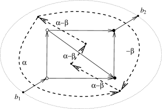
Figure 14. Directed planar network and its directed dual

Lemma 5.3.

The $2$-parametric family $\{\cdot,\cdot\}_{{\mathcal{F}}_{N}}$ is given by

$$\{y_{f},y_{f^{\prime}}\}_{{\mathcal{F}}_{N}}=\left(\sum_{e^{*}:f\to f^{\prime}}w^{*}(e^{*})-\sum_{e^{*}:f^{\prime}\to f}w^{*}(e^{*})\right)y_{f}y_{f^{\prime}}.$$

Proof.

Let $e=(u,v)$ be a directed edge. We say that the flag $(u,e)$ is positive, and the flag $(v,e)$ is negative. The color of a flag is defined as the color of the vertex participating in the flag.

Let $f$ and $f^{\prime}$ be two faces of $N$. We say that a flag $(v,e)$ is common to $f$ and $f^{\prime}$ if both $v$ and $e$ belong to $\partial f\cap\partial f^{\prime}$. Clearly, the bracket $\{y_{f},y_{f^{\prime}}\}_{{\mathcal{F}}_{N}}$ can be calculated as the sum of the contributions of all flags common to $f$ and $f^{\prime}$.

Assume that $(v,e)$ is a positive white flag common to $f$ and $f^{\prime}$, see Fig. 15. Then $y_{f}=\dfrac{x_{v}^{3}}{x_{v}^{2}}\bar{y}_{f}$ and $y_{f^{\prime}}=x_{v}^{1}x_{v}^{2}\bar{y}_{f^{\prime}}$, where $x_{v}^{i}$ are the weights of flags involving $v$ and $\{x_{v}^{i},\bar{y}_{f}\}_{\mathcal{R}}=\{x_{v}^{i},\bar{y}_{f^{\prime}}\}_{\mathcal{R}}=0$, see Section 3.2. Therefore, by (3.7), the contribution of $(v,e)$ equals $(\alpha_{12}-\alpha_{13}-\alpha_{23})y_{f}y_{f^{\prime}}$, which by (3.11) equals $-\alpha y_{f}y_{f^{\prime}}$.

Assume now that $(v,e)$ is a negative white flag common to $f$ and $f^{\prime}$, see Fig. 15. In this case $y_{f}=\dfrac{1}{x_{v}^{1}x_{v}^{3}}\bar{y}_{f}$ and $y_{f^{\prime}}=x_{v}^{1}x_{v}^{2}\bar{y}_{f^{\prime}}$, so the contribution of $(v,e)$ equals $(\alpha_{13}+\alpha_{23}-\alpha_{12})y_{f}y_{f^{\prime}}=\alpha y_{f}y_{f^{\prime}}$.

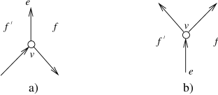
Figure 15. Contribution of a white common flag: a) positive flag; b) negative flag

In a similar way one proves that the contribution of a positive black flag common to $f$ and $f^{\prime}$ equals $-\beta y_{f}y_{f^{\prime}}$, and the contribution of a negative black flag common to $f$ and $f^{\prime}$ equals $\beta y_{f}y_{f^{\prime}}$. Finally, the contributions of positive and negative gray flags are clearly equal to zero.

The statement of the lemma now follows from the definition of the directed dual network. ∎

5.3. Compatibility theorem

Now we can formulate the main theorem of this section.

Theorem 5.4.

Any Poisson structure in the two-parameter family ${\mathcal{P}}_{\alpha,\beta}$ is compatible with the cluster algebra ${\mathcal{A}}_{G^{0}_{k}(n)}$.

Proof.

By Theorem 5.1, it is enough to choose an initial extended cluster and to compare the coefficient matrix of ${\mathcal{P}}_{\alpha,\beta}$ in the basis $\tau$ with the exchange matrix for this cluster.

To find the coefficient matrix of ${\mathcal{P}}_{\alpha,\beta}$ we define a special network $N(k,m)$ with $k$ sources and $m$ sinks. The graph of $N(k,m)$ has $km+1$ faces. Each bounded face is a hexagon; all bounded faces together form a $(k-1)\times(m-1)$ parallelogram on the hexagonal lattice. Edges of the hexagons are directed North, South-East and South-West. Each vertex of degree 2 on the left boundary of this parallelogram is connected to a source, and each vertex of degree 2 on the upper boundary of this parallelogram is connected to a sink. The remaining vertices of degree 2 on the lower and the right boundaries of the parallelogram are eliminated: two edges $u_{1}\to v\to u_{2}$ are replaced by one edge $u_{1}\to u_{2}$ and the intermediate vertex $v$ is deleted. The sources are labelled counterclockwise from 1 to $k$, sinks from $k+1$ to $n$. The faces are labelled by pairs $(ij)$ such that $i\in[1,k]$, $j\in[k+1,n]$. The unbounded faces are labelled $(1j)$ and $(in)$ except for one face, which is not labelled at all. The network $N(k,m)$ is defined by assigning a face weight $y_{ij}$ to each labelled face $(ij)$. Consequently, the directed dual network $N^{*}(k,m)$ forms the dual triangular lattice. All edges of $N^{*}(k,m)$ incident to the vertices $(ij)$, $i\in[2,k]$, $j\in[k+1,n-1]$ are of weight $\alpha-\beta$.

For an example of the construction for $k=3$, $m=4$ see Fig. 16. The edge weights of the dual network that are not shown explicitly are equal to $\alpha-\beta$.

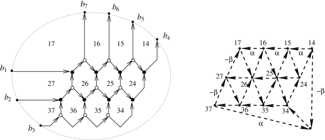
Figure 16. The graph of $N(3,4)$ and its directed dual $N^{*}(3,4)$

As the first step of the proof, we express the cluster variables $f_{ij}$ via the face weights of $N(k,m)$.

Lemma 5.5.

For any $i\in[1,k]$, $j\in[1,m]$, one has

$$f_{ij}=\pm\prod_{p=1}^{i}\prod_{q=j+k}^{n}y_{pq}^{1+\min\{i-p,q-j-k\}}.$$ (5.6)

Proof.

Since the graph of $N(k,m)$ is acyclic, one can use the Lindström lemma [Li] to calculate the minors of the boundary measurement matrix. Assume first that $i+j\leq n+1-k$. By (5.3) and the Lindström lemma, $f_{ij}$ equals to the sum of the products of the path weights for all $i$-tuples of nonintersecting paths between the sources $b_{1},b_{2},\dots,b_{i}$ and the sinks $b_{j+k},b_{j+k+1},\dots,b_{j+k+i-1}$, each product being taken with a certain sign. Note that there exists a unique path from $b_{1}$ to $b_{i+j+k-1}$ in $N(k,m)$. After this path is chosen, there remains a unique path from $b_{2}$ to $b_{i+j+k-2}$, and so on. Moreover, a path from $b_{1}$ to any sink $b_{p}$ with $p<i+j+k-1$ cuts off the sink $b_{i+j+k-1}$. Therefore, there exists exactly one $i$-tuple of paths as required. Relation (5.6) for $i+j\leq n+1-k$ now follows from the proof of Lemma 5.2.

The case $i+j\geq n+1-k$ is similar to the above one and relays on the uniqueness of an $(n+1-k-j)$-tuple of nonintersecting paths between the sources $b_{i+j+k-n},b_{i+j+k-n+1},\dots,b_{i}$ and the sinks $b_{j+k},b_{j+k+1},\dots,b_{n}$. Here we start with the unique path from $b_{i}$ to $b_{n}$, then choose the unique remaining path between $b_{i-1}$ and $b_{n-1}$, and so on. ∎

The next step is the calculation of $\tau$-coordinates for the initial extended cluster (5.4) via face weights.

Lemma 5.6.

The $\tau$-coordinates corresponding to the cluster variables of the initial extended cluster (5.4) are given by

$$\tau_{ij}=\pm y_{i+1,j+k-1},\qquad i\in[1,k-1],\;j\in[2,m].$$ (5.7)

Proof.

Combining the definition of $\tau$-coordinates via (5.2) and the description of the exchange matrix in the basis $\{f_{ij}\}$ provided by Fig. 13, we conclude that

$$\tau_{ij}=\frac{f_{i+1,j-1}f_{i,j+1}f_{i-1,j}}{f_{i,j-1}f_{i+1,j}f_{i-1,j+1}}=\frac{\dfrac{f_{i+1,j-1}}{f_{ij}}\cdot\dfrac{f_{ij}}{f_{i-1,j+1}}}{\dfrac{f_{i+1,j}}{f_{i,j+1}}\cdot\dfrac{f_{i,j-1}}{f_{i-1,j}}},\qquad i\in[1,k-1],\;j\in[2,m];$$

here we assume that $f_{ij}=1$ if $i=0$ or $j=m+1$. Next, by (5.6),

$$\frac{f_{ij}}{f_{i-1,j+1}}=\pm\prod_{p=1}^{i}\prod_{q=j+k}^{n}y_{pq}$$

for $i\in[1,k-1]$, $j\in[2,m]$, and the result follows. ∎

Remark 5.7.

The operation that expresses $\tau$-coordinates in terms of face weights is an analog of the twist studied in [BFZ1, FZ1].

The expressions for the $\tau$-coordinates that correspond to the stable variables of the initial extended cluster (5.4) are somewhat cumbersome. Recall that by (5.2), each stable variable enters the expression for the corresponding $\tau$-coordinate with some integer exponent $\varkappa_{ij}$. Let us denote

$$\tau^{*}_{ij}=\tau_{ij}f_{ij}^{-\varkappa_{ij}}$$

for $i=k$, $j\in[1,m]$ and $i\in[1,k]$, $j=1$.

Lemma 5.8.

The $\tau$-coordinates corresponding to the stable variables of the initial extended cluster (5.4) are given by

$$\tau^{*}_{ij}=\begin{cases}\pm\displaystyle\prod_{p=1}^{k-1}\;\prod_{q=j+k}^{\min\{n,j+k-p-1\}}y_{pq}\qquad&\text{for $i=k$, $j\in[2,m-1]$},\\ \pm\displaystyle\prod_{q=k+2}^{n}\;\prod_{p=i}^{\min\{n,i-q+k+2\}}y_{pq}\qquad&\text{for $i\in[2,k-1]$, $j=1$},\\ \pm\displaystyle\prod_{p=1}^{k-1}y_{pn}\qquad&\text{for $i=k$, $j=m$},\\ \pm\displaystyle\prod_{q=k+2}^{n}y_{1q}\qquad&\text{for $i=1$, $j=1$},\\ \pm\displaystyle\prod_{p=1}^{k}\prod_{q=k+1}^{n}y_{pq}^{-\min\{k-p,q-k-1\}}\qquad&\text{for $i=k$, $j=1$}.\end{cases}$$ (5.8)

Proof.

It suffices to note that

$$\tau^{*}_{ij}=\begin{cases}f_{k-1,j}/f_{k-1,j+1}\qquad&\text{for $i=k$, $j\in[2,m-1]$},\\ f_{i,2}/f_{i-1,2}\qquad&\text{for $i\in[2,k-1]$, $j=1$},\\ f_{k-1,m}\qquad&\text{for $i=k$, $j=m$},\\ f_{12}\qquad&\text{for $i=1$, $j=1$},\\ 1/f_{k-1,2}\qquad&\text{for $i=k$, $j=k+1$},\end{cases}$$

and to apply Lemma 5.5. ∎

To conclude the proof of the theorem we build the network $\Gamma_{\alpha,\beta}$ representing the family of Poisson brackets ${\mathcal{P}}_{\alpha,\beta}$ in the basis $\tau$. The vertices of $\Gamma_{\alpha,\beta}$ are $\tau$-coordinates $\tau_{ij}$, $i\in[1,n]$, $j\in[1,m]$. An edge from $\tau_{ij}$ to $\tau_{pq}$ with weight $c$ means that $\{\tau_{ij},\tau_{pq}\}_{{\mathcal{F}}_{N(k,m)}}=c\tau_{ij}\tau_{pq}$.

It follows immediately from Lemmas 5.3 and 5.6 that the induced subnetwork $\Gamma^{0}_{\alpha,\beta}$ of $\Gamma_{\alpha,\beta}$ spanned by the vertices $\tau_{ij}$, $i\in[1,k-1]$, $j\in[2,m]$ is isomorphic to the subnetwork $N_{0}^{*}(k,m)$ of $N^{*}(k,m)$ spanned by the vertices $(pq)$, $p\in[2,k]$, $q\in[k+1,n-1]$. We thus get an isomorphism between $\Gamma^{0}_{\alpha,\beta}$ and the corresponding induced subgraph of $\Gamma({\widetilde{B}})$, see Fig. 17. Under this isomorphism each edge of weight $\alpha-\beta$ is mapped to an edge of weight 1.

Figure 17. The isomorphisms between induced subgraphs of $\Gamma_{\alpha,\beta}$ and $\Gamma({\widetilde{B}})$

For the remaining vertices of $\Gamma_{\alpha,\beta}$, that is, $\tau_{ij}$, $i\in[1,k]$, $j=1$ or $i=k$, $j\in[1,m]$, we have to check the edges connecting them to the vertices of $\Gamma^{0}_{\alpha,\beta}$. Consider for example the case $i=k$, $j\in[2,m-1]$. Then, by Lemma 5.8, the bracket $\{\tau^{*}_{kj},\tau_{pq}\}_{{\mathcal{F}}_{N(k,m)}}$ for $\tau_{pq}\in\Gamma^{0}_{\alpha,\beta}$ is defined by the edges incident to the vertex subset of $N^{*}(k,m)$ corresponding to the factors in the right hand side of the first formula in (5.8), see Fig. 18. Clearly, any vertex $(p,q)\in N_{0}^{*}(k,m)$ other than $(k,j+k)$ and $(k,j+k-1)$ is connected to this subset by an even number of edges (more exactly, 0, 2, 4 or 6), all of them of weight $\alpha-\beta$. Since exactly half of the edges are directed to $(pq)$, the bracket between $y_{pq}$ and $\tau^{*}_{kj}$ vanishes by Lemma 5.3. The remaining two edges connecting the contracted set to the vertices $(k,j+k)$ and $(k,j+k-1)$ correspond to the two edges connecting the vertex $(k,j)$ to $(k-1,j)$ and $(k-1,j+1)$ in $\Gamma({\widetilde{B}})$, see Fig. 18.

Figure 18. The isomorphisms in the neighborhood of $\tau_{kj}$

Finally, factor $f_{kj}$ commutes with all $\tau_{pq}\in\Gamma^{0}_{\alpha,\beta}$. Indeed, given an edge between $\tau_{pq}\in\Gamma^{0}_{\alpha,\beta}$ and $y_{rs}$, define its degree as the exponent of $y_{rs}$ in expression (5.6) for $f_{kj}$. We have to prove that the sum of the degrees of all edges entering $\tau_{pq}$ equals the sum of the degrees of all edges leaving $\tau_{pq}$. This fact can be proved by analyzing all possible configurations of edges, see Fig. 19 presenting these configurations up to reflection.

Figure 19. Edges incident to $\tau_{pq}$ and their degrees

Other cases listed in Lemma 5.8 are treated in the same way. ∎

6. Acknowledgments

We wish to express gratitude to A. Postnikov who explained to us the details of his construction and to S. Fomin for stimulating discussions. M. G. was supported in part by NSF Grant DMS #0400484. M. S. was supported in part by NSF Grants DMS #0401178 and PHY#0555346. Authors were also supported by the BSF Grant # 2002375. A. V. is grateful to Centre Interfacultaire Bernoulli at École Polytechnique Fédérale de Lausanne for hospitality during his Spring 2008 visit. We are also grateful to the Institute of Advanced Studies of the Hebrew University of Jerusalem for the invitation to the Midrasha Mathematicae in May 2008, during which this paper was completed.

References

- [B] F. Brenti, Combinatorics and total positivity, J. Combin. Theory Ser. A 71 (1995), 175–218.
- [BFZ1] A. Berenstein, S. Fomin, and A. Zelevinsky, Parametrizations of canonical bases and totally positive matrices. Adv. Math. 122 (1996), 49–149.
- [BFZ2] A. Berenstein, S. Fomin, and A. Zelevinsky, Cluster algebras. III. Upper bounds and double Bruhat cells. Duke Math. J. 126 (2005), 1–52.
- [Fa] S. Fallat, Bidiagonal factorizations of totally nonnegative matrices, Amer. Math. Monthly, 108 (2001), 697–712.
- [Fo] S. Fomin, Loop-erased walks and total positivity, Trans. Amer. Math. Soc. 353 (2001), 3563–3583.
- [FG1] L. Faybusovich, M. I. Gekhtman, Elementary Toda orbits and integrable lattices, J. Math. Phys. 41 (2000), 2905–2921.
- [FG2] L. Faybusovich, M. I. Gekhtman, Poisson brackets on rational functions and multi-Hamiltonian structure for integrable lattices, Phys. Lett. A 272 (2000), 236–244.
- [FZ1] S. Fomin and A. Zelevinsky, Double Bruhat cells and total positivity. J. Amer. Math. Soc. 12 (1999), 335–380.
- [FZ2] S. Fomin and A. Zelevinsky, Total Positivity: tests and parametrizations., Math. Inteligencer. 22 (2000), 23–33.
- [FZ3] S. Fomin and A. Zelevinsky, Cluster algebras.I. Foundations. J. Amer. Math. Soc. 15 (2002), 497–529.
- [GSV1] M. Gekhtman, M. Shapiro, and A. Vainshtein, Cluster algebras and Poisson geometry. Mosc. Math. J. 3 (2003), 899–934.
- [GSV2] M. Gekhtman, M. Shapiro, and A. Vainshtein, Cluster algebras and Weil-Petersson forms. Duke Math. J. 127 (2005), 291–311.
- [GSV3] M. Gekhtman, M. Shapiro, and A. Vainshtein, Poisson geometry of directed networks in an annulus, arXiv: 0901.0020.
- [GSV4] M. Gekhtman, M. Shapiro, and A. Vainshtein, Bäcklund-Darboux transformations for Toda flows from cluster algebra perspective, in preparation.
- [GSV5] M. Gekhtman, M. Shapiro, and A. Vainshtein, Inverse problem for 1-1 networks in an annulus, in preparation.
- [GrSh] B. Grünbaum and G. Shephard, Rotation and winding numbers for planar polygons and curves. Trans. Amer. Math. Soc. 322 (1990), 169–187.
- [HKKR] T. Hoffmann, J. Kellendonk, N. Kutz and N. Reshetikhin Factorization dynamics and Coxeter-Toda lattices, Comm. Mat. Phys. 212 (2000), 297–321.
- [KM] S. Karlin, J. McGregor,Coincidence Probabilities, Pacific J. Math. 9 (1959), 1141–1164.
- [LP] T. Lam, P. Pylyavskyy, Total positivity in loop groups I: whirls and curls, arXiv:0812.0840.
- [Li] B. Lindström, On the vector representations of induced matroids, Bull. London Math. Soc. 5 (1973), 85–90.
- [Lu] G. Lusztig, Total positivity in reductive groups. Lie theory and geometry, 531–568, Progr. Math. 123, Birkhäuser, Boston, 1994.
- [M] J. Moser, Finitely many mass points on the line under the influence of the exponential potential - an integrable system. Dynamical systems, theory and applications, 467–497, Lecture Notes in Physics 38, Springer, Berlin, 1975.
- [P] A. Postnikov, Total positivity, Grassmannians and networks, arXiv: math/0609764.
- [R] N. Reshetikhin Integrability of characteristic Hamiltonian systems on simple Lie groups with standard Poisson Lie structure, Comm. Mat. Phys. 242 (2003), 1–29.
- [ReST] A. Reyman and M. Semenov-Tian-Shansky Group-theoretical methods in the theory of finite-dimensional integrable systems Encyclopaedia of Mathematical Sciences, vol.16, Springer–Verlag, Berlin, 1994 pp. 116–225.
- [S] J. Scott, Grassmannians and cluster algebras, Proc. London Math. Soc. 92 (2006), 345–380.
- [T] K. Talaska, A formula for Plücker coordinates associated with a planar network, Int. Math. Res. Not. 2008, 19pp.