ExoFit: orbital parameters of extra-solar planets from radial velocities
Abstract
Retrieval of orbital parameters of extrasolar planets poses considerable statistical challenges. Due to sparse sampling, measurement errors, parameters degeneracy and modelling limitations there are no unique values of basic parameters such as period and eccentricity. Here we estimate the orbital parameters from radial velocity data in a Bayesian framework by utilising Markov Chain Monte Carlo (MCMC) simulations with the Metropolis-Hastings algorithm. We follow a methodology recently proposed by Gregory and Ford. Our implementation of MCMC is based on the object oriented approach outlined by Graves. We make our resulting code, ExoFit, publicly available with this paper. It can search for either one or two planets as illustrated on mock data. As an example we re-analysed the orbital solution of companions to HD 187085 and HD 159868 from the published radial velocity data. We confirm the degeneracy reported for orbital parameters of the companion to HD 187085 and show that a low eccentricity orbit is more probable for this planet. For HD 159868 we obtained slightly different orbital solution and a relatively high ‘noise’ factor indicating the presence of an unaccounted signal in the radial velocity data. ExoFit is designed in such a way that it can be extended for a variety of probability models, including different Bayesian priors.
keywords:
stars:planetary systems - stars: individual: HD 187085, HD 159868 - techniques: radial velocities - methods: data analysis - methods: statistical - methods: numerical.1 Introduction
The study of extra-solar planets is of great importance because it helps us to understand the origin and evolution of the Solar System. The information gained from analysing new stellar systems serves as a sign post towards finding possible life forms outside our Solar System. The first 200 or so detected extra-solar planets has been discovered using the radial velocity method. Other detection methods include astrometric method, transit photometry, gravitational micro-lensing and direct imaging. Astrometric method look for the periodic shifts in the position of star and transit method measures the attenuation of star light caused by the passage of the planet across the star. Gravitational micro-lensing utilises the amplification of light rays from the background object by a an intervening massive object. In a number of cases, existence of the planet has been confirmed by more than one method. The number of multi-planet systems discovered has also increased during the past few years due the improved precision of radial velocity measurements.
In this article, we are concerned with the extraction of orbital parameters from observed radial velocity data. A survey of the literature in this field indicates that orbital parameters and their uncertainties were traditionally obtained by a two step method. Searching for periodicity in the radial velocity data using a Lomb-Scargle (Lomb, 1976; Scargle, 1982) periodogram to fix the orbital period and then estimating other parameters by Levenberg-Marquardt (Levenberg, 1944; Marquardt, 1963) minimisation. Recently, Bayesian methods have been applied (Gregory, 2005a; Ford, 2005; Ford & Gregory, 2007) to find out the best fit orbital parameters and these studies suggest that Bayesian techniques have considerable advantages over the traditional methods; for e.g when the data does not cover a single orbital phase of the planet. In this work we analyse the radial velocity data from a Bayesian point of view and extract the orbital parameters and corresponding uncertainties using Markov Chain Monte Carlo (MCMC) simulations. We make our code, ExoFit, and a detailed documentation available on-line111http://www.star.ucl.ac.uk/lahav/exofit.html.
The outline of the paper is as follows. In Section 2 we summarise the modelling of radial velocities. In Section 3 we discuss the Bayesian approach to the problem. In Section 4 we present the MCMC implementation and the ExoFit software package. ExoFit is then applied to mock and observed data in Sections 5 and 6 respectively. The results are discussed in Section 7.
2 Modelling of Radial Velocity
2.1 Doppler Spectrography
Planets are many times fainter than their host stars because they shine only by reflecting the star light. This makes their direct imaging extremely difficult. However, the gravitational pull of the planet makes the star wobble and this produces measurable periodic shifts in the apparent speed of the parent star. The motion of the star around the centre of mass causes the observed spectrum of the star to be Doppler shifted according its radial velocity, i.e. the velocity along the line of sight of the observer. This is measured over a course of time to obtain the radial velocity data along with the measurement uncertainties.
2.2 Radial Velocity of Star
A single planet model is assumed here to analyse the radial velocity data. The radial velocity of a star can be written as (Murray & Dermott, 2000; Ohta et al., 2005)
| (1) | |||||
where is the th radial velocity entry corresponding to time coordinate and,
the systematic velocity of the system,
the mass of the planet,
the mass of the star,
the mean motion and is orbital period of planet,
the length of the semi-major axis of the planet,
the inclination of the orbital plane with the ecliptic,
the eccentricity of the planet,
the true anomaly at time and
the longitude of periastron.
The radial velocity depends on time via the true anomaly .
The full formalism and comparison with a common approximation is discussed in the User’s Guide to ExoFit.
2.3 Radial velocity data
According to (http://exoplanet.eu) eighteen different radial velocity search programmes are looking for extrasolar planets. Majority of the contributions come from Keck, Lick and Anglo-Australian observatories (the California & Carnegie and Anglo-Australian planet searches) and searches based at l’Observatoire de Haute Provence and La Silla Observatory (the Geneva extrasolar planet search). Radial velocity data for a star consists of time of observation , measured radial velocity and uncertainty associated with each measurement . These uncertainties are a characteristic of the instruments used for measurements. The precision of these instruments have improved from the order of in 1994 to order of (Butler et al, 2006; Pepe et al., 2004) at present.222The measurement method and its uncertainties are discussed in the corresponding planet discovery papers. This is extremely significant for finding low mass companions as well as planets with large s.
3 Bayesian Retrieval of orbital parameters
3.1 Introduction
The extraction of orbital parameters from the radial velocity data poses considerable statistical challenges. Earlier in this article we mentioned the traditional two step method that is generally used to retrieve orbital parameters. Studies by Cumming (2004) and Cumming et al. (1999) have identified two cases where these methods become inefficient in accurately characterising the orbital elements:
-
1.
When the orbital period is extremely short and the eccentricity is high.
-
2.
When the duration of observation does not span at least a single orbital phase.
Incomplete radial velocity data gives rise to a multitude of orbital solutions which is referred to as parameter degeneracy. Since the transit probability of the planet increases for short periods, the orbital parameters predicted by the periodogram method can be verified, in some cases, with the help of transit photometry. Higher eccentricities make the radial velocity curve less sinusoidal. O’Toole et al. (2007) makes use of a 2DKLS periodogram to incorporate the effect of eccentricity of the orbits while searching for orbital periods. Recently Bayesian techniques have been employed by Gregory (2005a), Ford (2005) and Ford & Gregory (2007) to retrieve the orbital parameters of extra-solar planets. The results show that Bayesian methods tackle the difficulties associated with the traditional methods efficiently and transparently. We emphasise that the relative merit of different methods depends on the quality of the data. Broadly speaking the choice of prior distribution may change the inference (posterior distribution) significantly when the quality of data is poor.
3.2 The Bayesian method
The starting point of any Bayesian analysis is Bayes’ theorem (Bayes, 1763). Let be a vector of observations whose probability distribution is conditional on parameters , where represents the background information or the hypothesis by which the probability statements are made. Suppose that the parameter has the probability distribution . Then, Bayes’ theorem says
| (2) |
For a continuous we can write
| (3) |
which is constant for given and a probability distribution . Then Equation [2] can be rewritten as
| (4) |
In the above equation is called prior distribution of since it conveys our knowledge about before the data has been observed. Correspondingly, is known as the posterior distribution of given . The factor is a normalising constant which ensures that the posterior distribution integrates to one. We call the likelihood function of since can be considered as a function of instead of . Then,
| (5) |
Statistical inferences regarding are derived from the posterior distribution of . The posterior distribution encapsulates all information about unknown quantities following the observation of the data . The principal steps in the Bayesian method can be involve the Likelihood , the prior , the posterior , and the resulting inference, e.g. O’Hagan & Forster (2004).
3.3 Likelihood function
Let represent the measured radial velocity data for the th instant of time . Observed radial velocity data can be modelled by the equation (Gregory, 2005a)
| (6) |
where is the true radial velocity of the star and is the uncertainty component arising from accountable but unequal measurement errors which are assumed to be normally distributed. The term explains any unknown measurement errors. There can be multiple reasons for the presence of this uncertainty component (Butler et al, 2006). For example this could be the result of another planet in the system or caused by the intrinsic anomalies in the star spectrum due to the irregularities on the surface of the star (Pepe et al., 2004; Mayor et al., 2003; Bouchy et al., 2005). Thus any noise component that cannot be modelled is described by the term . The probability distribution of is chosen to be a Gaussian distribution with finite variance . Therefore the combination of uncertainties has a Gaussian distribution with a variance equal to .
3.4 Choice of Priors
The choice of priors is extremely important in the Bayesian analysis as senseless choice of priors can produce to misleading results. Physical and geometric conditions govern the selection of prior distributions for most of the parameters. Since the prior distribution in our problem can be written as
| (9) | |||||
on the assumption that they are independent. We will discuss how the above conditions are met for our choice of prior for each parameter in the next few sections.
We follow the choice of priors as given by Ford & Gregory (2007), as summarized in Table 1. Obviously, part of the Bayesian framework is the ability to change priors and to check the sensitivity of the results to them. Our ExoFit package allows this freedom.
| Para. | Prior | Mathematical Form | Min | Max |
|---|---|---|---|---|
| Jeffreys | 0.2 | 15000 | ||
| Mod. Jeffreys | 0.0 | 2000 | ||
| Uniform | -2000 | 2000 | ||
| Uniform | 1 | 0 | 1 | |
| Uniform | 0 | |||
| Uniform | 1 | 0 | 1 | |
| Mod. Jeffreys | 0 |
3.5 Posterior Distribution
Posterior distribution is obtained by applying the Bayes’ theorem given by the equation (4). Useful and interesting features of the posterior distribution should be identified before making summary statements. For example, the posterior distribution may be unimodal but asymmetric or it can be multi-modal with many probability peaks. Any summary statistic(e.g. mean, median and mode) can be expressed in terms of posterior expectations of (Gilks et al., 1996; Berger, 1980).
4 MCMC Implementation
4.1 The MCMC approach
Difficulty in evaluating the multi-dimensional integrals is an inherent inability of any Bayesian formulation. Many techniques have been developed in the last 25 years to deal with this problem. Simulation methods dominate this area and several computational algorithms were developed to numerically integrate the posterior distribution in order to find out the marginal distributions of each parameter. According to Berg (2004) the abundance of computational power has produced a paradigm shift with respect to statistics: Computationally intensive but conceptually simple methods are preferred. Markov Chain Monte Carlo (MCMC) method is one of the most commonly used methods for simulating complex probability distributions333A general form this method given by Metropolis-Hastings (Metropolis et al., 1953; Hastings, 1970) algorithm is explained in ExoFit User Guide.. Our code is based on the concepts outlined by Graves (2007). The emphasis is on the extensibility of the code to accommodate different probability models to a certain extent.
Bayesian MCMC methods have gained popularity in various areas of astrophysics, for example in multi-parameter estimation from cosmological data sets (e.g. CosmoMC; Lewis & Bridle (2002)). We emphasise that the two ingredients, the Bayesian approach and the MCMC tool, are distinct and not necessarily related. One may apply MCMC to a multi-parameter likelihood analysis (i.e. without priors– equivalent to a Bayesian method for uniform priors). On the other hand one may work out a full Bayesian method (with complicated priors) using a grid-based maximisation procedure, without the need for MCMC. Having said that, the combination of the Bayesian and MCMC methods is a very powerful way to tackle our problem.
From a Bayesian point of view analysis of statistical problems requires an efficient tool for simulating posterior densities and MCMC methods are ideally suited for this purpose. In general, one must consider planet-planet interaction while modelling radial velocity of a star. In typical systems the radial velocity of an -planet model can be approximated as a linear combination of single planet radial velocities. With the present version of ExoFit it is possible to search for either one or two planets.
4.2 The ExoFit software package
ExoFit is a step towards achieving the goals mentioned above. It should be considered as a platform to develop MCMC based methods for estimating orbital parameters of a generalised multi-planet model. Object oriented design of ExoFit makes it extremely well suited for extending the analysis to multi-planet systems with prior constraints on several orbital parameters such as eccentricity and length of semi-major axis. Following Graves (2007), our implementation MCMC consists of Data, State, Bond and Update. They are referred to as objects in object oriented analysis. data handles the input data into the MCMC analysis. A state consists of a set of parameters whose posterior distribution is sought. The parameter values at a particular instant defines the state of Markov Chain in the analysis. The parameters in a particular state are connected to each other by a bond. It consists of prior densities and likelihood. For each state there corresponds a bond strength which is equal to . In other words it is the posterior density without the normalisation constant in Bayes’ theorem. An update selects the parameters that should be updated at particular iteration. New values for the parameters are proposed according to the update defined and the new bond strength is then calculated for the proposed state. The new state is accepted or rejected according Metropolis-Hastings method.
The central concept of this approach is that, the MCMC engine remains the same and need not be re-implemented whenever the probability model gets changed. We also take advantage of the commonalities among the different components of MCMC. Our implementation works for variety or prior distributions () and Update methods. The only component that requires to be changed is the likelihood function.
Convergence is an important aspect of any MCMC method and the choice of proposal distribution is absolutely crucial for achieving convergence of the chain. Choosing an effective proposal distribution is very difficult in many cases. ExoFit employs an adaptive Metropolis algorithm described by Haario et al. (1999) to fine tune the proposal distribution step sizes.
5 Application to mock data
We used simulated data sets to test the accuracy of the orbital parameters extracted by ExoFit. The output of ExoFit is analysed with the help of the R statistical environment444http://www.r-project.org/ which is freely available. A number of packages are available in R for checking the convergence of Markov Chains and creating the histograms and density plots of posterior distribution of parameters.
| 1-planet | 2-planets | ||||
|---|---|---|---|---|---|
| 1400.15200 | -17.90 | 2.1 | -25.30 | 2.1 | |
| 1413.87749 | -18.50 | 2.8 | -18.20 | 2.8 | |
| 1434.46573 | -30.00 | 1.4 | -22.50 | 1.4 | |
| 1455.05396 | -33.00 | 2.0 | -26.20 | 2.0 | |
| 1489.36769 | -41.10 | 2.1 | -52.70 | 2.1 | |
| 1496.23043 | -41.30 | 2.4 | -50.80 | 2.4 | |
| 1503.09318 | -45.50 | 1.7 | -51.20 | 1.7 | |
| 1564.85788 | -47.60 | 1.7 | -45.30 | 1.7 | |
| 1571.72063 | -44.20 | 2.0 | -46.80 | 2.0 | |
| 1585.44612 | -39.40 | 1.6 | -50.70 | 1.6 | |
| 1592.30886 | -33.60 | 1.9 | -44.70 | 1.9 | |
| 1612.89710 | -14.50 | 1.9 | -14.70 | 1.9 | |
| 1619.75984 | -6.17 | 1.9 | -3.07 | 1.9 | |
| 1654.07357 | 38.20 | 2.4 | 45.30 | 2.4 | |
| 1688.38729 | 61.90 | 1.6 | 50.30 | 1.6 | |
| 1695.25004 | 64.90 | 1.7 | 54.90 | 1.7 | |
| 1715.83827 | 74.00 | 2.9 | 75.30 | 2.9 | |
| 1722.70102 | 73.70 | 2.7 | 78.00 | 2.7 | |
| 1736.42651 | 70.20 | 1.8 | 78.00 | 1.8 | |
| 1743.28925 | 72.70 | 2.6 | 81.10 | 2.6 | |
| 1770.74024 | 67.30 | 2.3 | 65.50 | 2.3 | |
| 1777.60298 | 65.10 | 2.0 | 57.80 | 2.0 | |
| 1784.46573 | 66.20 | 2.7 | 55.20 | 2.7 | |
| 1798.19122 | 61.90 | 2.4 | 53.40 | 2.4 | |
| 1811.91671 | 56.70 | 1.9 | 56.00 | 1.9 | |
| 1818.77945 | 56.20 | 2.2 | 58.80 | 2.2 | |
| 1832.50494 | 51.00 | 1.7 | 58.20 | 1.7 | |
| 1901.13239 | 32.80 | 1.6 | 25.90 | 1.6 | |
| 1907.99514 | 32.40 | 2.0 | 29.60 | 2.0 | |
| 1921.72063 | 29.80 | 2.2 | 33.70 | 2.2 | |
| 1928.58337 | 33.90 | 3.7 | 40.10 | 3.7 | |
| 1935.44612 | 29.10 | 2.9 | 36.80 | 2.9 | |
| 1962.89710 | 19.00 | 2.2 | 22.40 | 2.2 | |
| 1969.75984 | 17.40 | 2.2 | 16.30 | 2.2 |
| Parameter | Planet 1 | ExoFit | ExoFit | ExoFit | Planet 2 | ExoFit | ExoFit | ExoFit |
|---|---|---|---|---|---|---|---|---|
| Mean | Median | Mode | Mean | Median | Mode | |||
| 12.0 | ||||||||
| 700.00 | ||||||||
| 60.00 | ||||||||
| 0.38 | ||||||||
| 3.10 | ||||||||
| 0.67 | ||||||||
5.1 1-planet data with 1-planet fit
In this The first set of radial velocity entries as shown in Table 2 (columns 1, 2 and 3) is created using a single planet model (equation (2.2)) and adding a Gaussian noise. Table 3 shows the input parameters used to create the data set and the parameters obtained with ExoFit for a single planet search. Three posterior summary statistics are compared in Table 3; where column 2 gives the assumed input values, column 3 contains the mean values of MCMC samples for each parameter along with the sample standard deviation, column 4 shows the median values with 75% and 25% quantiles. We used Hyndman (1996)’s method to calculate Highest Density Regions (HDRs) of the posterior distribution. Column 5 contains posterior modes (maximum a posteriori) and associated 68.3% credible regions. The difference between actual radial velocity curve and the radial velocity curve for the parameters obtained from ExoFit is shown in the Fig. 2. We also plot the deviation of the radial velocities from the actual one for each of these orbital solutions in Fig. 2. We note the deviations between the estimators are smaller than . The noise factor is less than the measurement uncertainties, implying the assumed radial velocity model is “good” and there is no sign of an additional signal present in the data.
5.2 2-planet data with 1-planet fit
A second set of radial velocity entries as shown in column 4 of Table 2 has been created by adding the radial velocity from a second planet with orbital parameters as shown in Table 3 to the radial velocity data of the single planet model in column 2 of Table 2. The results from the application of to this simulated data is shown in columns 7, 8 and 9 of Table 3. Noise factor in this case is clearly higher than the measurement uncertainties, indicating the presence of a signal unaccounted for in the radial velocity model. Note that the noise factor obtained in the previous case was only . Fig. 3 shows the radial velocity curve for the median values of the posterior distribution of orbital parameters from along with the actual radial velocity plot for the 2-planet model.


5.3 A 2-planet fit to 2-planet mock data
has an option to search for two planets in the radial velocity data. We choose the probability model to be similar to that of the single planet model explained in Section 3.3. The observed radial velocity data is again modelled by the equation 6. The radial velocity predicted by the mathematical model at an instant is given by
| (10) |
11 parameters 555Subscripts 1 and 2 indicate planets 1 and 2 respectively., as defined in the Section 2.2 are used to fit the above equation onto the radial velocity data. The likelihood function is again given by equations 7 and 8 respectively, and becomes the parameter in our probability model. The choice of prior distributions for each of these parameters is given in Table 4.
| Para. | Prior | Mathematical Form | Min | Max |
|---|---|---|---|---|
| Uniform | -2000 | 2000 | ||
| Jeffreys | 0.2 | 15000 | ||
| Mod. Jeffreys | 0.0 | 2000 | ||
| Uniform | 1 | 0 | 1 | |
| Uniform | 0 | |||
| Uniform | 1 | 0 | 1 | |
| Jeffreys | 0.2 | 15000 | ||
| Mod. Jeffreys | 0.0 | 2000 | ||
| Uniform | 1 | 0 | 1 | |
| Uniform | 0 | |||
| Uniform | 1 | 0 | 1 | |
| Mod. Jeffreys | 0 |
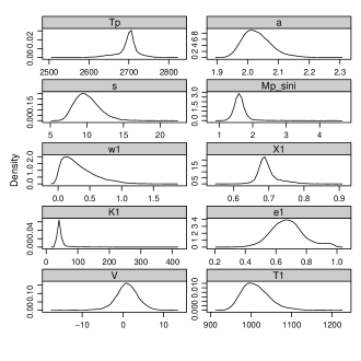
We apply the to the 2-planet mock radial velocity data given in Table 2 (column 4). A comparison of actual orbital parameters with the ones extracted with is given in Table 5. Fig 4 shows the actual radial velocity curve and the one created with the median values of the posterior distribution of orbital parameters obtained from 666We caution that, using median values for orbital parameters with skewed marginal posterior distributions can lead to models that very poor..Note that the noise factor is now compared to in the single planet model. The density plots are shown in Fig 5.
| Parameter | Actual | ExoFit | ExoFit | ExoFit |
|---|---|---|---|---|
| Mean | Median | Mode | ||

Constraining the longitude of periastron becomes increasingly difficult when the eccentricity of planetary system approaches zero. Ford (2006) suggests that, the efficiency of MCMC sampler in this situation can be increased by adopting a new parametrisation with and . For discussions about further improvements in parametrisation, choice of priors and proposal distributions for MCMC, see Ford (2006). These considerations will be implemented in the future version of ExoFit.
6 Application to observed data
In this section we apply ExoFit to published radial velocity data. We choose data sets in which the measurement noise is relatively high and the entries are poorly sampled. The following examples shows that ExoFit does a good job in estimating the posterior distribution orbital parameters.
6.1 The companion to HD 187085
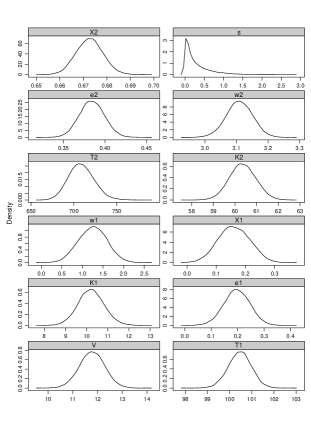
Detection of a planet orbiting HD 187085 was announced in 2006 with 40 epoch of radial velocity measurements between 1998 November and 2005 October (Jones et al., 2006). It has reported that although an orbital solution of period 986 days and eccentricity 0.47 gave the best fit, a solution with low eccentricity also produced similar fit to the observed data. Application of ExoFit revealed the posterior density distribution orbital parameters as shown in Fig. 6.
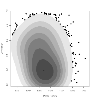
The MCMC values with iterations are shown in the user’s manual. It is evident from Fig. 6 that the posterior density of eccentricity is a heavily skewed . The joint probability distributing of orbital period and eccentricity is shown in Fig. 7 with two dimensional HDRs. From these plots it is reasonable to conclude that the data clearly favours a low eccentricity orbit.
Table 6 shows the summary statistics of the posterior distribution of orbital parameters of HD 187085 along with the published results. The eccentricity is from the mean, median and mode respectively, compared with the published estimate . 777For a posterior distribution that is approximately Gaussian (e.g.. parameter T), estimates like mean, median and mode will yield nearly the same values. However, when the posterior density is not Gaussian and exhibit skewness (e.g.. parameter ) mean, median and mode will differ significantly. Since this is the case for parameter , posterior median and and mode will be a better estimate than posterior mean. If the posterior distribution has more than one peak, posterior modes provide ideal summary of the distribution. Keplerian orbital solutions for HD 187085 from Table 6 shown in Fig. 8.
How sensitive are the results to the assumed priors? In Table 7 we show results based on 10 trial runs of for Gregory’s priors (Table 1) and for Top Hat priors, i.e. uniform between the same lower and upper values as in Gregory’s priors. This indicates the data and assumed model are ‘good’. The role of priors would be more dramatic in the case of poor data.
| Parameter | ExoFit | ExoFit | ExoFit | Jones et al |
|---|---|---|---|---|
| Mean | Median | Mode | ||
| 986 | ||||
| 17 | ||||
| 0.47 | ||||
| 94 | ||||
| (JD -2450000) | 912 | |||
| 0.75 | ||||
| 2.05 |

| HD 187085 | HD 187085 | HD159868 | HD159868 | ||
|---|---|---|---|---|---|
| Parameter | Gregory’s | Top Hat | Gregory’s | Top Hat | |
| T (days) | |||||
| K | |||||
| V | |||||
| e | |||||
| s | |||||
| (JD -2450000) | |||||
| a |
6.2 The companion to HD 159868
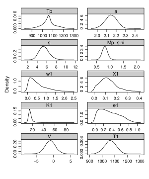
Orbital parameters of a planet orbiting HD 159868 from 28 radial velocity measurements was reported on 2007 by O’Toole et al. (2007). They employed a two-dimensional periodogram to search for the optimum orbital period and the eccentricity for the orbit. The posterior distribution of parameters are shown in Fig. 9 and since they are nearly symmetric, we choose median of the distribution as the point statistic. Table 8 shows the median of samples from and the Keplerian orbit obtained is plotted in Fig. 10 along with the observed data and uncertainties. Table 7 shows the sensitivity to changing the priors to Top Hat. We note that the ‘noise’ factor is 10 times larger than the measurement errors, probably indicating the presence of an unaccounted signal in the radial velocity data.
| Parameter | ExoFit | ExoFit | ExoFit | O’Toole et al |
|---|---|---|---|---|
| Mean | Median | Mode | ||
| T (days) | ||||
| K | ||||
| V | ||||
| e | ||||
| – | ||||
| s | – | |||
| (JD -2450000) | ||||
| a |

7 Discussion
We present a new software package, ExoFit, for estimating the orbital parameters from radial velocity data in a Bayesian framework by utilising Markov Chain Monte Carlo (MCMC) simulations with the Metropolis-Hastings algorithm. ExoFit can search for one or two planets in a given radial velocity data and can easily be extended to search for more planets. We applied to simulated data sets to check the accuracy of the parameters extracted. As an illustration we re-analysed the orbital solution of companions to HD 187085 and HD 159868 from the published radial velocity data. We confirm the degeneracy reported for orbital parameters of the companion to HD 187085 and show that a low eccentricity orbit is more probable for this planet. For HD 159868 we obtained slightly different orbital solution and a relatively high ‘noise’ factor indicating the presence of an unaccounted signal in the radial velocity data. We have also studied the sensitivity of the results to changes in the Bayesian priors. We plan to extend ExoFit to search for more than two planets and to analyse transit photometry data.
8 Acknowledgements
We are grateful to Jean-Philippe Beaulieu, Farah Islam, David Kipping, Yasushi Suto and Giovanna Tinetti for helpful discussions. SB acknowledges a Royal Astronomical Society studentship grant and OL acknowledges a Royal Society Wolfson Research Merit Award.
References
- Bayes (1763) Bayes T., 1763, Philosophical Transactions of the Royal Society, 53, 370
- Berg (2004) Berg B. A., 2004, Markov Chain Monte Carlo Simulations And Their Statistical Analysis: With Web-based Fortran Code. World Scientific
- Berger (1980) Berger J. O., 1980, Statistical Decision Theory and Bayesian Analysis, 2 edn. Springer-Verlag New York Inc, 175 Fifth Avenue, New York, NY10010, USA
- Bouchy et al. (2005) Bouchy F., Bazot M., Santos N. C., 2005, A&A, 440, 609
- Butler et al (2006) Butler et al R. P., 2006, ApJ, 646, 505
- Cumming (2004) Cumming A., 2004, MNRAS, 354, 1165
- Cumming et al. (1999) Cumming A., Marcy G. W., Butler R. P., 1999, ApJ, 526, 890
- Ford (2005) Ford E. B., 2005, AJ, 129, 1706
- Ford (2006) Ford E. B., 2006, ApJ, 642, 505
- Ford & Gregory (2007) Ford E. B., Gregory P. C., 2007, Statistical Challenges in Modern Astronomy IV, ASP Conference Series, 371, 189
- Gilks et al. (1996) Gilks W. R., Richardson S., Spiegelhalter D. J., eds, 1996, Markov Chain Monte Carlo in Practice. Chapman & Hall London
- Graves (2007) Graves T. L., 2007, Journal of Computational & Graphical Statistics, 16, 24
- Gregory (2005a) Gregory P. C., 2005a, ApJ, 631, 1198
- Gregory (2005b) Gregory P. C., 2005b, Bayesian Logical Data Analysis for the Physical sciences: A comparitive Approch with “Mathematica” Support. Cambridge: Cambridge University Press
- Haario et al. (1999) Haario H., Saksman E., Tamminen J., 1999, Computational Statistics, 14, 375
- Hastings (1970) Hastings W. K., 1970, Biometrika, 57, 97
- Hyndman (1996) Hyndman R. J., 1996, The American Statistician, 50, 120
- Jones et al. (2006) Jones H. R. A., Butler R. P., Tinney C. G., Marcy G. W., Carter B. D., Penny A. J., McCarthy C., Bailey J., 2006, MNRAS, 369, 249
- Levenberg (1944) Levenberg K., 1944, Quarterly of Applied Mathematics, 2, 164
- Lewis & Bridle (2002) Lewis A., Bridle S., 2002, Phys. Rev. D, 66, 103511
- Lomb (1976) Lomb N. R., 1976, Ap&SS, 39, 447
- Marquardt (1963) Marquardt D., 1963., SIAM Journal on Applied Mathematics, 11, 431
- Mayor et al. (2003) Mayor M., Pepe F., Queloz D., Bouchy F., Rupprecht G., Lo Curto G., Avila G., Benz W., Bertaux J.-L., Bonfils X., Dall T., Dekker H., 2003, The Messenger, 114, 20
- Metropolis et al. (1953) Metropolis N., Rosenbluth A. W., Rosenbluth M. N., H. T. A., Teller E., 1953, Journal of Chemical Physics, 21, 1087
- Murray & Dermott (2000) Murray C. D., Dermott S. F., 2000, Solar System Dynamics. Cambridge University Press
- O’Hagan & Forster (2004) O’Hagan A., Forster J., 2004, Bayesian Inference, 2 edn. Vol. 2B of Kendall’s Advanced Theory of Statistics, Oxford University Press Inc, 198 Madison Avenue, New York, NY10016
- Ohta et al. (2005) Ohta Y., Taruya A., Suto Y., 2005, ApJ, 622
- O’Toole et al. (2007) O’Toole S. J., Butler R. P., Tinney C. G., Jones H. R. A., Marcy G. W., Carter B., McCarthy C., Bailey J., Penny A. J., Apps K., Fischer D., 2007, ApJ, 660, 1636
- Pepe et al. (2004) Pepe F., Mayor M., Queloz et al D., 2004, A&A, 423, 385
- Scargle (1982) Scargle J. D., 1982, ApJ, 263, 835