New cubature formulae and hyperinterpolation
in three variables

Abstract

A new algebraic cubature formula of degree $2n+1$ for the product Chebyshev measure in the $d$-cube with $\approx n^{d}/2^{d-1}$ nodes is established. The new formula is then applied to polynomial hyperinterpolation of degree $n$ in three variables, in which coefficients of the product Chebyshev orthonormal basis are computed by a fast algorithm based on the 3-dimensional FFT. Moreover, integration of the hyperinterpolant provides a new Clenshaw-Curtis type cubature formula in the 3-cube.

1 Introduction.

A cubature formula with high accuracy is an important tool for numerical computation and has various applications. One of the applications is to construct polynomial hyperinterpolation, introduced by Sloan [17], which is an approximation process constructed by applying the cubature formula on the Fourier coefficients of the orthogonal projection operator.

A cubature formula of degree $2n-1$ with $N$ nodes with respect to a measure $d\mu$ supported on a set $\Omega$ takes the form

$$\int_{\Omega}{p(x)\,d\mu}=\sum_{\xi\in X_{m}}{w_{\xi}\,p(\xi)}\qquad\mbox{for all}\quad p\in\Pi_{2n-1}^{d}(\Omega)\;,$$ (1)

where $\{w_{\xi}\}$, called weights, are (positive) numbers, $X_{n}$ is a set of points, called nodes,

$$\xi:=(\xi_{1},\xi_{2},\ldots,\xi_{d})\in X_{n}\subset\Omega$$ (2)

with $\mathrm{card}(X_{n})=N$, and $\Pi_{m}^{d}$ denoted the subspace of $d$-variate polynomials of total degree $\leq m$ restricted to $\Omega$. For a cubature formula of degree $2n-1$ to exist, it is necessary that

$$N:=\mbox{card}(X_{n})\geq\mbox{dim}(\Pi_{n}^{d}(\Omega))={n+d\choose d}=\frac{n^{d}}{d!}(1+o(1)).$$ (3)

There are improved lower bounds of the same order in terms of $n$. A challenging problem is to construct cubature formulae with fewer nodes, that is, with the number of nodes $N$ close to the lower bound.

In this paper we consider the case that the measure is given by the product Chebyshev weight function

$$d\mu=W_{d}(x)\,dx,\qquad W_{d}(x):=\frac{1}{\pi^{d}}\prod_{i=1}^{d}\frac{1}{\sqrt{1-x_{i}^{2}}}$$ (4)

on the cube $\Omega:=[-1,1]^{d}$. For $d=1$, the Gaussian quadrature formula of degree $2n-1$ needs merely $N=n$ points. Our main result is a new family of cubature formulae that uses $N\approx n^{d}/2^{d-1}$ many nodes. For $d=2$ these formulae are known to have minimal number of nodes. For $d\geq 3$ they are still far from the lower bound, but they appear to be the best ones that are known at this moment. We refer to Section 2 for further discussions. We present numerical tests on these cubature formulae in three variables and also apply them to constructing polynomial hyperinterpolation operator in three variables.

For every function $f\in C(\Omega)$ the $\mu$-orthogonal projection of $f$ on $\Pi_{n}^{d}(\Omega)$ is

$$\mathcal{S}_{n}f(x)=\sum_{|\alpha|\leq n}{a_{\alpha}\,p_{\alpha}(x)},\qquad a_{\alpha}:=\int_{\Omega}{f(x)\,p_{\alpha}(x)\,d\mu}\;,$$ (5)

where $x=(x_{1},x_{2},\ldots,x_{d})$ is a $d$-dimensional point, $\alpha$ is a $d$-index of length $|\alpha|$

$$\alpha=(\alpha_{1},\ldots,\alpha_{d})\in\mathbb{N}^{d},\qquad|\alpha|:=\alpha_{1}+\ldots+\alpha_{d}\;,$$ (6)

and the set of polynomials $\{p_{\alpha}\,,\,0\leq|\alpha|\leq n\}$ is any $\mu$-orthonormal basis of $\Pi_{n}^{d}(\Omega)$ with $p_{\alpha}$ of total degree $|\alpha|$ (concerning the theory of multivariate orthogonal polynomials, we refer the reader to the monograph [9]). Clearly, $\mathcal{S}_{n}p=p$ for every $p\in\Pi_{n}^{d}(\Omega)$. Given a cubature formula (1) of degree $\leq 2n$, we obtain from (5) the polynomial approximation of degree $n$ by the discretized Fourier coefficients $\{{c}_{\alpha}\}$

$$f(x)\approx\mathcal{L}_{n}f(x):=\sum_{|\alpha|\leq n}{{c}_{\alpha}\,p_{\alpha}(x)}\;,\;\;{c}_{\alpha}:=\sum_{\xi\in X_{n}}{w_{\xi}\,f(\xi)\,p_{\alpha}(\xi)}\;,$$ (7)

where ${c}_{\alpha}=a_{\alpha}$ and thus $\mathcal{L}_{n}p=\mathcal{S}_{n}p=p$ for every $p\in\Pi_{n}^{d}(\Omega)$. This is the hyperinterpolation operator. It satisfies the basic estimate: for every $f\in C(\Omega)$,

$$\|f-\mathcal{L}_{n}f\|_{L_{d\mu}^{2}(\Omega)}\leq 2\sqrt{\mu(\Omega)}\,E_{n}(f)\to 0\;,\;\;n\to\infty\;,$$ (8)

where $E_{n}(f):=\inf{\{\|f-p\|_{\infty}\,,\,\,p\in\Pi_{n}^{d}(\Omega)\}}$, so that it converges in mean. The convergence rate can be estimated by a multivariate version of Jackson theorem (see, for example, [15]), which shows that $E_{n}(f)=\mathcal{O}(n^{-p})$ for $f\in C^{p}(\Omega)$, $p\in\mathbb{R}^{+}$. It becomes an effective approximation tool in the uniform norm when its operator norm (the so-called Lebesgue constant) grows slowly (cf. [16, 18, 11, 5]). The hyperinterpolation has been used effectively in several cases: originally for the sphere [16, 18], and more recently for the square [4, 5], the disk [11], and the cube [6]. We will use our new cubature formulae to construct a hyperinterpolation operator of three variables for the Chebyshev weight function on the cube. We show that the computation can be carried out efficiently using the 3-dimensional FFT and that the algorithm can be completely vectorized. We will also present numerical results on hyperinterpolation of several test functions.

The paper is organized as follows. In Section 2 we construct new cubature formulae and report results of numerical tests, where comparisons are made with tensor-product Gauss-Chebyshev formulae. Hyperinterpolation in three variables is considered in Section 3, where we show how to compute it effectively and report the results of numerical tests. Finally in Section 4, we obtain a new (nontensorial) Clenshaw-Curtis type formula in the cube by integrating the hyperinterpolant in Section 3 and show that it has a clear superiority over tensorial Clenshaw-Curtis and Gauss-Legendre cubature on nonentire test integrands, a phenomenon known for 1-dimensional and 2-dimensional Clenshaw-Curtis formulae (see [20, 19]).

2 Algebraic cubature for the $d$-dimensional Chebyshev measure.

We consider cubature formula for the product Chebyshev weight function (4), which is normalized so that its integral over $[-1,1]^{d}$ is $1$. For $d=1$, we write $w(x)=W_{1}(x)$.

Let $\Pi_{n}^{d}$ denote the space of polynomials of total degree $\leq n$ in $d$ variables. We write $\Pi_{n}$ if $d=1$. The Gaussian quadrature formula for $w$ takes the form

$$\int_{-1}^{1}f(x)w(x)dx=\frac{1}{n}\sum_{k=1}^{n}f(\cos\tfrac{(2k-1)\pi}{2n})\;,\qquad\forall f\in\Pi_{2n-1}\;.$$ (9)

For $d=2$, a cubature formula of degree $2n-1$ needs at least (cf. [13])

$$N^{*}=\dim(\Pi_{n-1}^{2})+\left\lfloor\frac{n}{2}\right\rfloor=\frac{n(n+1)}{2}+\left\lfloor\frac{n}{2}\right\rfloor$$ (10)

many nodes. Cubature formulae that attain this lower bound can be constructed for the product Chebyshev weight $W_{2}(x)$ (see [14, 22] and the references therein) by studying common zeros of associated orthogonal polynomials. In [1], these cubature rules were derived by an elementary method which depends on a factorization of the Gauss-Lobatto quadrature into two sums, over even indices and odd indices, respectively. This factorization method was also used for $d>2$ in [1] and yields a cubature formula of degree $2n-1$ for $W_{d}$ with roughly $n^{d}/2^{d/2}$ many nodes.

A close inspection of the factorization method shows that it actually allows us to derive cubature formulae of degree $2n-1$ for $W_{d}$ with roughly $2(n/2)^{d}$ many nodes. This number of nodes is substantially less than $n^{d}$ of the product cubature formula or $n^{d}/2^{d/2}$ of the formulae in [1], although it likely far from optimal as seen from (3).

We start with the Gauss-Lobatto formula for $w$ on $[-1,1]$. It takes the form

$$\int_{-1}^{1}f(x)w(x)dx=\frac{1}{n}\left(\frac{1}{2}f(-1)+\sum_{j=1}^{n-1}f\left(\cos\tfrac{j\pi}{n}\right)+\frac{1}{2}f(1)\right):=I_{n}f\;,$$ (11)

which again holds for all $f\in\Pi_{2n-1}$. We proceed to factor this rule into two terms. The factorization depends on whether $n$ is even or $n$ is odd. Define

$$n=2m:\qquad\begin{split}&I^{E}_{n}f:=\frac{1}{n}\left(\frac{1}{2}f(-1)+\sum_{j=1}^{m-1}f\left(\cos\tfrac{2j\pi}{n}\right)+\frac{1}{2}f(1)\right)\\ &I^{O}_{n}f:=\frac{1}{n}\sum_{j=1}^{m}f\left(\cos\tfrac{(2j-1)\pi}{n}\right)\end{split}$$ (12)

and define

$$n=2m-1:\qquad\,\begin{split}&I^{E}_{n}f:=\frac{1}{n}\left(\sum_{j=1}^{m-1}f\left(\cos\tfrac{2j\pi}{n}\right)+\frac{1}{2}f(1)\right)\\ &I^{O}_{n}f:=\frac{1}{n}\left(\frac{1}{2}f(-1)+\sum_{j=1}^{m-1}f\left(\cos\tfrac{(2j-1)\pi}{n}\right)\right)\;,\end{split}$$ (13)

where we use the superscripts $E$ and $O$ to signify that the sum is taken over even indices or odd indices, respectively. Evidently, the quadrature (11) becomes

$$\int_{-1}^{1}f(x)w(x)dx=I^{E}_{n}f+I^{O}_{n}f\;,\qquad\forall f\in\Pi_{2n-1}\;,$$

by definition.

The Chebyshev polynomials, $T_{n}$, are orthogonal with respect to $w$ on $[-1,1]$,

$$T_{n}(t):=\cos n{\theta}\;,\qquad\quad t=\cos{\theta}\;.$$

The following elementary lemma plays a key role in constructing cubature formulae on $[-1,1]^{d}$.

Lemma 2.1

For $n\geq 0$ and $k\in{\mathbb{Z}}$,

$$I^{E}_{n}T_{k}=\begin{cases}0,&k\neq 0\mod n\\ \frac{1}{2},&k=0\mod n\end{cases}\quad\hbox{and}\quad I^{O}_{n}T_{k}=\begin{cases}0,&k\neq 0\mod n\\ \frac{1}{2},&k=0,2n,4n,\ldots\\ -\frac{1}{2},&k=0,n,3n,\ldots.\end{cases}$$

Proof. The proof follows from elementary trigonometric identities. For example, for $n=2m$, an elementary calculation shows that

$$I^{O}_{n}T_{k}=\frac{1}{n}\sum_{j=1}^{m}\cos k\tfrac{(2j-1)\pi}{2m}=\frac{\sin k\pi}{4m\sin\frac{k\pi}{2m}}=\frac{\sin k\pi}{2n\sin\frac{k\pi}{n}}$$

from which $I^{O}_{n}T_{k}=0$ for $k\neq 0\mod n$ follows immediately. The case when $k$ is a multiple of $n$ follows from the first equal sign of the above equation without summing it up. Similarly,

$$I^{E}_{n}T_{k}=\frac{1}{n}\left(\frac{1}{2}\cos k\pi+\sum_{j=1}^{m-1}\cos k\tfrac{j\pi}{m}+\frac{1}{2}\right)=\frac{\sin k\pi\cos\frac{k\pi}{n}}{2n\sin\frac{k\pi}{n}}\;,$$

from which the stated result follows. The proof for $n=2m-1$ is similar and is omitted for brevity.     q.e.d.

Let ${\sigma}\in\{E,O\}^{d}$, that is,

$${\sigma}=({\sigma}_{1},\ldots,{\sigma}_{d})\;\mbox{with}\;{\sigma}_{i}=E\;\mbox{or}\;{\sigma}_{i}=O.$$

For a function $f:{\mathbb{R}}^{d}\mapsto{\mathbb{R}}$, we define the sum

$$I_{n}^{{\sigma}_{1}}\cdots I_{n}^{{\sigma}_{d}}f$$

as a $d$-fold multiple sum in which $I^{{\sigma}_{k}}$ is applied to the $k$-th variable of $f$. Let us define

$$\tilde{{\sigma}}_{i}=\left\{\begin{array}[]{ll}E&{\sigma}_{i}=O\\ O&{\sigma}_{i}=E\end{array}\right.\;$$ (14)

For each ${\sigma}\in\{E,O\}^{d}$, we then define

$$I_{n,d}^{\sigma}f:=I_{n}^{{\sigma}_{1}}\ldots I_{n}^{{\sigma}_{d}}f+{I}_{n}^{\widetilde{{\sigma}}_{1}}\ldots{I}_{n}^{\widetilde{{\sigma}}_{d}}f\;.$$

Since the sum introduces a symmetry among ${\sigma}\in\{E,O\}^{d}$, there are $2^{d-1}$ distinct $I_{n,d}^{\sigma}f$ sums.

Theorem 2.2

For $d\geq 1$ and each ${\sigma}\in\{E,O\}^{d}$, the cubature formula

$$\int_{[-1,1]^{d}}f(x)W_{d}(x)dx=2^{d-1}I_{n,d}^{\sigma}f$$ (15)

is exact for $f\in\Pi_{2n-1}^{d}$ and its number of nodes, $N$, satisfies

$$N=2\left(\left\lfloor\frac{n}{2}\right\rfloor\right)^{d}(1+o(n^{-1}))\;.$$

Proof. For $k=(k_{1},\ldots,k_{d})\in{\mathbb{N}}_{0}^{d}$ let $T_{k}(x):=T_{k_{1}}(x_{1})\cdots T_{k_{d}}(x_{d})$, which is a polynomial of total degree $|k|:=k_{1}+\cdots+k_{d}$. It suffices to establish (15) for $f\in\{T_{k}:|k|\leq 2n-1\}$, since this set is an orthogonal basis of $\Pi_{n}^{d}$. In this case we have

$$\int_{[-1,1]^{d}}T_{k}(x)W_{d}(x)dx=2^{d-1}\left[I_{n}^{{\sigma}_{1}}T_{k_{1}}\cdots I_{n}^{{\sigma}_{d}}T_{k_{d}}+I_{n}^{\widetilde{{\sigma}}_{1}}T_{k_{1}}\cdots I_{n}^{\widetilde{{\sigma}}_{d}}T_{k_{d}}\right]\;.$$

By the orthogonality of $T_{k}$, the left hand side is equal to 1 if $k=(0,\ldots,0)$ and zero if $k\neq(0,\ldots,0)$. From the definition of $I^{E}_{n}$ and $I^{O}_{n}$, it is evident that $I^{E}_{n}1=I^{O}_{n}1=1/2$. Hence, for $k=(0,\ldots,0)$, the right hand side is equal to $2^{d-1}(2^{-d}+2^{-d})=1$, verifying the equation for $k=(0,\ldots,0)$.

Assume now $0<|k|\leq 2n-1$. If one of $k_{i}\neq 0\mod n$, then $I_{n,d}^{{\sigma}}T_{k}=0$ by Lemma 2.1. We are left with the case that $k_{i}=0\mod n$ for all $i$. Since $|k|\leq 2n-1$, there can be at most one $k_{i}=n$. Furthermore, $|k|>0$ shows that there is exactly one $k_{i}=n$. Thus the right hand side becomes $I_{n}^{{\sigma}_{i}}T_{n}+I_{n}^{\widetilde{{\sigma}}_{i}}T_{n}=I^{E}_{n}T_{n}+I^{O}_{n}T_{n}$, which is zero as $I^{E}_{n}T_{n}=1/2$ and $I^{O}_{n}T_{n}=-1/2$ according to the Lemma 2.1.     q.e.d.

For the case of $d=2$, Theorem 2.2 contains two distinct cubature formulae for ${\sigma}=(E,E),\,(E,O)$, respectively, whose number of nodes are either equal to $N^{*}$ in (10) or $N^{*}+1$, those are the ones that have appeared in [14, 22], and later in [1], as mentioned earlier. For $d=3$, there are 4 distinct formulae for ${\sigma}=(E,E,E),\,(E,E,O),\,(E,O,E),\,(O,E,E)$, respectively. For $n=2m$, the number of nodes is

$$N=\frac{(n+1)^{3}+(n+1)}{4}$$

for ${\sigma}=(E,E,E)$ and

$$N=\frac{(n+1)^{3}-(n+1)}{4}$$

for ${\sigma}=(E,E,O),\,(E,O,E),\,(O,E,E)$, respectively.

In order to demonstrate the effectiveness of the new cubature formula, we present in Figures 1-2 numerical results of (15) with $\sigma=(E,E,E)$ on the integrals of six text functions with respect to the product Chebyshev measure on the 3-cube. The first three functions are analytic entire (a polynomial, an exponential and a gaussian), whereas the other three are less smooth: one analytic but not entire (a 3-dimensional version of the Runge test function), one $C^{\infty}$ nonanalytic, and one $C^{2}$. These functions are analogues of test functions for algebraic cubature in dimension 1 and 2, see [20, 19]. We compare them with two natural choices for cubature on a tensor product domain: the tensor-product Gauss-Chebyshev and Gauss-Chebyshev-Lobatto formulae. The results, obtained with Matlab (cf. [10]), demonstrate the superiority of the new formula in all cases, especially for the less smooth functions, in terms of number of function evaluations. It should be pointed out that, however, the superiority for the less smooth functions arises for even $n$ (a sort of parity phenomenon). Other numerical tests (not reported for brevity) have shown that the cubature formula has the same behavior for ${\sigma}=(E,E,O),\,(E,O,E),\,(O,E,E)$.

A natural question associated with cubature formulae is polynomial interpolation. Let $X_{n-1}$ denote the set of the nodes of the cubature formula (15). The interpolation problem looks for a polynomial subspace, ${\mathcal{S}}$, of the lowest degree such that

$$P(x)=f(x),\qquad x\in X_{n-1},\quad\forall f\in C({\mathbb{R}}^{d})$$

has a unique solution in ${\mathcal{S}}$. In the case of $d=2$, this problem is completely solved in [22], where ${\mathcal{S}}$ is a subspace of $\Pi_{n}^{2}$ which includes $\Pi_{n-1}^{2}$, and compact formulae of the fundamental interpolation polynomials are also given there. For $d>2$, however, the problem is much harder, since the number of nodes of our cubature is far from $\dim(\Pi_{n}^{d})$. For example, if $d=3$, then $\dim(\Pi_{n-1}^{d})=n(n+1)(n+2)/6\approx n^{3}/6$, whereas our cubature has $\approx n^{3}/4$ many nodes. The problem essentially comes down to study the polynomial ideal that has $X_{n-1}$ as its variety (see [23]).

A simpler approach to polynomial approximation via these new nodes is given by hyperinterpolation, as described in the Introduction. In the next section we shall apply such a method in the 3-dimensional case.

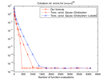
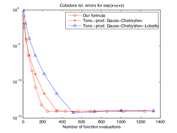
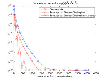
Figure 1: Relative cubature errors versus the number of function evaluations for three test functions.

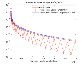
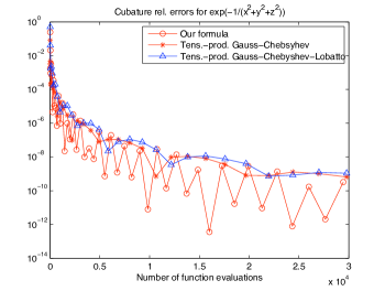
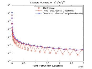
Figure 2: Relative cubature errors versus the number of function evaluations for three test functions.

3 Implementing hyperinterpolation in the 3-cube.

We now use cubature formula (15) to construct hyperinterpolation as in (7) for the 3-cube $\Omega=[-1,1]^{3}$. In this case, $\{p_{\alpha}\}$ is the product Chebyshev orthonormal basis (cf. [9]), i.e.

$$p_{\alpha}(x)=\hat{T}_{\alpha_{1}}(x_{1})\hat{T}_{\alpha_{2}}(x_{2})\hat{T}_{\alpha_{3}}(x_{3})\;,$$ (16)

where $\hat{T}_{k}(\cdot)=\sqrt{2}\cos(k\arccos(\cdot)),\;k>0$ and $\hat{T}_{0}(\cdot)=1$. Moreover, let

$$C_{n}=\left\{\cos{k\pi\over n},\;k=0,...,n\right\}\;$$

be the set of $n+1$ Chebyshev-Lobatto points, and $C_{n}^{E}$, $C_{n}^{O}$ its restriction to even and odd indices, respectively. Then,

$$X_{n}=\left(C_{n+1}^{{\sigma}_{1}}\times C_{n+1}^{{\sigma}_{2}}\times C_{n+1}^{{\sigma}_{3}}\right)\;\cup\;\left(C_{n+1}^{\tilde{{\sigma}}_{1}}\times C_{n+1}^{\tilde{{\sigma}}_{2}}\times C_{n+1}^{\tilde{{\sigma}}_{3}}\;\right)\,,$$ (17)

with $({\sigma}_{1},{\sigma}_{2},{\sigma}_{3})\in\{E,O\}^{3}$, see (14). The weights of the cubature formula (15) for $\xi\in X_{n}$, are

$$w_{\xi}=\frac{4}{(n+1)^{3}}\cdot\left\{\begin{array}[]{ll}1&\mbox{if}\;\xi\;\mbox{is an interior point}\\ {1/2}&\mbox{if}\;\xi\;\mbox{is a face point}\\ {1/4}&\mbox{if}\;\xi\;\mbox{is an edge point}\\ {1/8}&\mbox{if}\;\xi\;\mbox{is a vertex point}\\ \end{array}\right.$$ (18)

Note that, since

$$\mbox{dim}(\Pi_{n}^{3}(\Omega))={(n+1)(n+2)(n+3)/6}<N=\mbox{card}(X_{n})\approx n^{3}/4\;,$$

the polynomial $\mathcal{L}_{n}f$ in (7) is not interpolant.

Now, defining

$$F(\xi)=F(\xi_{1},\xi_{2},\xi_{3})=\left\{\begin{array}[]{ll}w_{\xi}f(\xi)&\xi\in X_{n}\\ \\ 0&\xi\in(C_{n+1}\times C_{n+1}\times C_{n+1})\backslash X_{n}\end{array}\right.$$ (19)

we can write

$$c_{\alpha} = \sum_{\xi\in X_{n}}w_{\xi}f(\xi)p_{\alpha}(\xi)$$

$$= \sum_{\xi_{1}\in C_{n+1}}\left(\sum_{\xi_{2}\in C_{n+1}}\left(\sum_{\xi_{3}\in C_{n+1}}F(\xi_{1},\xi_{2},\xi_{3})\,\hat{T}_{\alpha_{1}}(\xi_{1})\right)\hat{T}_{\alpha_{2}}(\xi_{2})\right)\hat{T}_{\alpha_{3}}(\xi_{3})$$

$$= \left(\prod_{s=1}^{3}{\beta_{\alpha_{s}}}\right)\,\sum_{i=0}^{n+1}\left(\sum_{j=0}^{n+1}\left(\sum_{k=0}^{n+1}F_{ijk}\cos{k\alpha_{1}\pi\over n+1}\right)\cos{j\alpha_{2}\pi\over n+1}\right)\cos{i\alpha_{3}\pi\over n+1}\;,$$

where

$$\alpha=(\alpha_{1},\alpha_{2},\alpha_{3})\in\{0,1,\dots,n\}^{3}\;,\;\;\beta_{\alpha_{s}}=\left\{\begin{array}[]{ll}\sqrt{2}&\alpha_{s}>0\\ 1&\alpha_{s}=0\end{array}\right.\;,\;\;s=1,2,3\;.$$

This shows that the 3-dimensional coefficients array $\{c_{\alpha}\}$ is a scaled Discrete Cosine Tranform of the 3-dimensional array

$$F_{ijk}=F\left(\cos{i\pi\over n+1},\cos{j\pi\over n+1},\cos{k\pi\over n+1}\right)\;,\;\;0\leq i,j,k\leq n\;,$$ (20)

where we eventually pick up only the $(n+1)(n+2)(n+3)/6\approx n^{3}/6$ hyperinterpolation coefficients corresponding to $|\alpha|=\alpha_{1}+\alpha_{2}+\alpha_{3}\leq n$.

A fast implementation of hyperinterpolation is now feasible (for example in Matlab), via the FFT. Indeed, we have written a Matlab code (see [8]), completely vectorized by several implementation tricks, whose kernel can be summarized as follows: Algorithm: Fast total degree hyperinterpolation in the 3-cube

• construct the hyperinterpolation point set $X_{n}$ as union of the two subgrids in (17);

• compute the cubature weights in (18);

• compute the 3-dimensional array $\{F_{ijk}\}$ at the complete grid $C_{n+1}\times C_{n+1}\times C_{n+1}$ by (19) (notice that $f$ is evaluated only at $X_{n}$);

• compute the 3-dimensional array of coefficients $\{c_{\alpha}\}$ by three nested applications of the 1-dimensional $\mbox{Real}(\mbox{FFT}(\cdot))$ operator;

• select the coefficients $\{c_{\alpha}\}$ corresponding to the triples $\alpha=(\alpha_{1},\alpha_{2},\alpha_{3})$ such that $|\alpha|=\alpha_{1}+\alpha_{2}+\alpha_{3}\leq n$.

We recall that there is a simple way to approximate a function in the 3-cube by tensor-product of polynomials of degree $n$, that is, by a tensor-product discrete Chebyshev series (ultimately a tensor-product hyperinterpolant). Such an approximation uses $(n+1)^{3}$ function evaluations, and $(n+1)^{3}$ coefficients. In contrast, let us stress again the following facts on our total-degree hyperinterpolation of degree $n$ in the 3-cube: Remark

• the number of hyperinterpolation nodes, or function evaluations, is equal to $\mbox{card}(X_{n})\approx n^{3}/4$;

• the number of hyperinterpolation coefficients is $\mbox{dim}(\Pi_{n}^{3})\approx n^{3}/6$.

In order to compare the performances of total-degree and tensor-product hyperinterpolation in the 3-cube, we show, in the following figures, the hyperinterpolation errors versus both the number of nodes and the number of coefficients on the six test functions already used in Section 2, and we choose again $({\sigma}_{1},{\sigma}_{2},{\sigma}_{3})=(E,E,E)$, see (17). The errors are relative to the maximum deviation of the function from its mean and are computed on a uniform control grid. Since the computation of the coefficients via the FFT has roughly the same cost for both kinds of hyperinterpolation, we have chosen the number of function evaluations as a measure of computational cost for the construction, and the number of coefficients as a measure of the compression capability of the algorithms.

The situation here is in some sense opposite to that of Figures 1-2. Indeed, total-degree appears superior to tensor-product hyperinterpolation on the smoothest functions, but not on the less smooth ones. As it is natural from the observation above, the behavior of total-degree hyperinterpolation in terms of number of coefficients is better than that in terms of number of nodes (function evaluations).

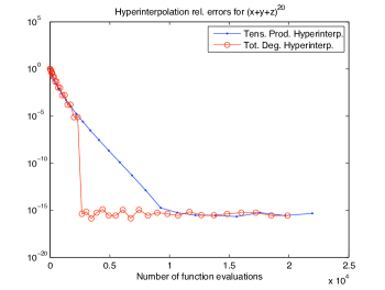
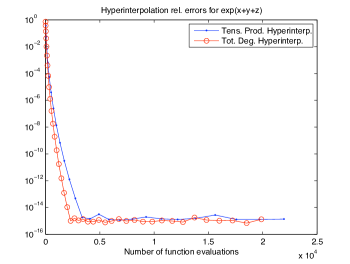
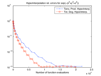
Figure 3: Hyperinterpolation relative errors versus the number of function evaluations for three entire test functions.

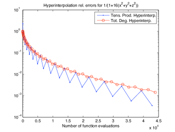
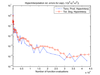
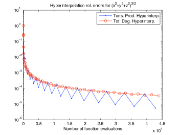
Figure 4: Hyperinterpolation relative errors versus the number of function evaluations for three nonentire test functions.

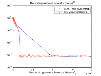
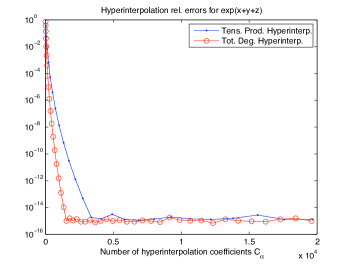
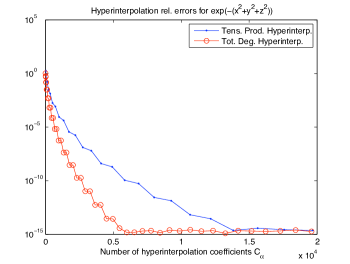
Figure 5: Hyperinterpolation relative errors versus the number of hyperinterpolation coefficients for three entire test functions.

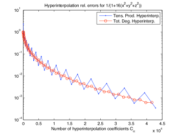
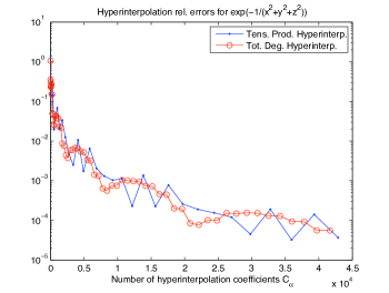
Figure 6: Hyperinterpolation relative errors versus the number of hyperinterpolation coefficients for three nonentire test functions.

4 A Clenshaw-Curtis-like formula in the cube.

In the recent paper [19], perusing an idea already present in [17], it has been shown how hyperinterpolation allows us to construct new cubature formulae. Given $h\in L^{2}_{d\mu}(\Omega)$ and $f\in C(\Omega)$, we can approximate the integral of $hf$ in $d\mu$ as

$$\int_{\Omega}{h(x)\,f(x)\,d\mu} \approx\int_{\Omega}{h(x)\,\mathcal{L}_{n}f(x)\,d\mu}$$

$$=\sum_{|\alpha|\leq n}{c_{\alpha}\,m_{\alpha}}=\sum_{{\xi}\in X_{n}}{\lambda_{\xi}\,f({\xi})}\;,$$ (21)

where the generalized “orthogonal moments” $\{m_{\alpha}\}$ and the cubature weights $\{\lambda_{\xi}\}$ are defined by

$$m_{\alpha}:=\int_{\Omega}{h(x)\,p_{\alpha}(x)\,d\mu}\;,\;\;\lambda_{\xi}:=w_{\xi}\sum_{|\alpha|\leq n}{p_{\alpha}(\xi)\,m_{\alpha}}\;.$$ (22)

Observe that the cubature formula (4) is exact for every $f\in\Pi_{n}^{d}(\Omega)$, and that $\{m_{\alpha}\}$ are just Fourier coefficients of $h$ with respect to the $\mu$-orthonormal basis $\{p_{\alpha}\}$.

Concerning stability and convergence of such cubature formulae, the following result has been proved in [19]:

Theorem 4.1

Let all the assumptions for the construction of the cubature formula (4) be satisfied, and in particular let $h\in L^{2}_{d\mu}(\Omega)$. Then the sum of the absolute values of the cubature weights has a finite limit

$$\lim_{n\to\infty}{\sum_{{\xi}\in X_{n}}{\left|\lambda_{\xi}\right|}}=\int_{\Omega}{|h(x)|\,d\mu}\;.$$ (23)

Notice that (23) ensures that the sum of absolute values of the weights is bounded, and thus by recalling that $\mathcal{L}_{n}$ is a projection operator on $\Pi^{d}_{n}(\Omega)$ we obtain the Polya-Steklov type (cf. [12]) convergence estimate

$$\left|\int_{\Omega}{h(x)\,f(x)\,d\mu}-\sum_{{\xi}\in X_{n}}{\lambda_{\xi}\,f({\xi})}\right|\leq\left(\int_{\Omega}{|h(x)|\,d\mu}+\sup_{n}{\sum_{{\xi}\in X_{n}}{\left|\lambda_{\xi}\right|}}\right)\,E_{n}(f)\;,$$ (24)

where $E_{n}(f)$ denotes the error of the best polynomial approximation of degree $n$ to $f$ in the uniform norm.

Now, applying (4)-(22) in the case

$$d\mu=w(x)\,dx\;,\;\;w\in L^{1}_{dx}(\Omega)\;,\;\;\mbox{with}\;\;h=\frac{1}{w}\in L^{1}_{dx}(\Omega)\;,$$ (25)

(since then $h^{2}=1/w^{2}\in L^{1}_{d\mu}(\Omega)$) we obtain, via hyperinterpolation, a cubature formula for the standard Lebesgue measure from an algebraic cubature formula for another measure (absolutely continuos with respect to the former). The specialization of this approach to the $1$-dimensional Chebyshev measure gives ultimately the popular Clenshaw-Curtis quadrature formula [7]. An extension to dimension 2 has been studied in [19]. Here we apply the method in dimension 3, obtaining a new nontensorial Clenshaw-Curtis-like cubature formula in the 3-cube.

In Figures 7-8 we display the relative errors of such a formula for $({\sigma}_{1},{\sigma}_{2},{\sigma}_{3})=(E,E,E)$ (cf. (17)) on the six test functions already used above, compared with those of the tensor-product Clenshaw-Curtis, Gauss-Legendre, and Gauss-Legendre-Lobatto formulae. The numerical results have been obtained with Matlab, using [10] for the Gaussian formulae and [21] for the tensor-product Clenshaw-Curtis formula.

In particular, we see that with the entire test functions nontensorial Clenshaw-Curtis cubature is more accurate than the tensor-product version, but less accurate than the other two tensor-product formulae. On the other hand, in the less smooth cases the nontensorial Clenshaw-Curtis formula is better than all the other three, especially for odd hyperinterpolation degrees $n$, which correspond to use $n+1$ even in (15) (again a sort of parity phenomenon, cf. Figure 2). This behavior echos that of 1-dimensional and 2-dimensional Clenshaw-Curtis formulae (see [20, 19]). Other numerical tests (not reported for brevity) have shown that the other versions of the nontensorial Clenshaw-Curtis formula, corresponding to $(\sigma_{1},\sigma_{2},\sigma_{3})=(E,E,O),\,(E,O,E),\,(O,E,E)$ in (17), produce essentially the same results.

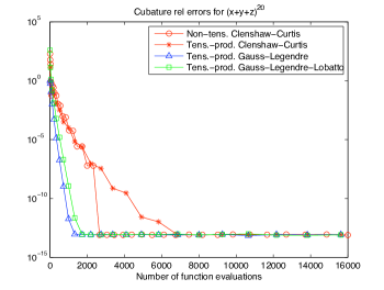
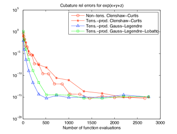
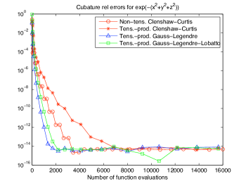
Figure 7: Relative cubature errors versus the number of cubature points for three test functions.

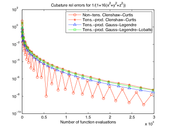
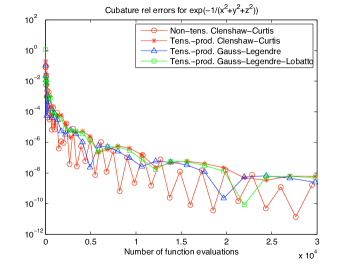
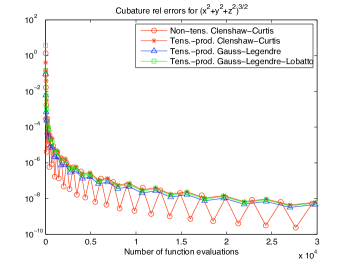
Figure 8: Relative cubature errors versus the number of cubature points for three test functions.

References

- [1] B. Bojanov and G. Petrova, On minimal cubature formulae for product weight functions, J. Comp. Appl. Math. 85 (1997), 113–121.
- [2] L. Bos, M. Caliari, S. De Marchi, M. Vianello and Y. Xu, Bivariate Lagrange interpolation at the Padua points: The generating curve approach, J. Approx. Theory 143 (2006), 15–25.
- [3] L. Bos, S. De Marchi, M. Vianello and Y. Xu, Bivariate Lagrange interpolation at the Padua points: The ideal theory approach, Numer. Math. 108 (2007), 43–57.
- [4] M. Caliari, S. De Marchi, R. Montagna and M. Vianello, HYPER2D: a numerical code for hyperinterpolation at Xu points on rectangles, Appl. Math. Comput. 183 (2006), 1138-1147.
- [5] M. Caliari, S. De Marchi and M. Vianello, Hyperinterpolation on the square, J. Comput. Appl. Math. 210 (2007), 78–83.
- [6] M. Caliari, S. De Marchi and M. Vianello, Hyperinterpolation in the cube, Comput. Math. Appl. 55 (2008), 2490–2497.
- [7] C.W. Clenshaw and A.R. Curtis, A method for numerical integration on an automatic computer, Numer. Math. 2 (1960), 197–205.
- [8] S. De Marchi and M. Vianello, Hyper3: a Matlab code for fast polynomial hyperinterpolation in the 3-cube (preliminary version available at: http://profs.sci.univr.it/demarchi/software.html).
- [9] C.F. Dunkl and Y. Xu, Orthogonal Polynomials of Several Variables, Encyclopedia of Mathematics and its Applications, vol. 81, Cambridge University Press, Cambridge, 2001.
- [10] W. Gautschi, Orthogonal Polynomials: Computation and Approximation, Numerical Mathematics and Scientific Computation, Oxford Science Publications, Oxford University Press, New York, 2004.
- [11] O. Hansen, K. Atkinson and D. Chien, On the norm of the hyperinterpolation operator on the unit disk and its use for the solution of the nonlinear Poisson equation, IMA J. Numer. Anal., published online 20 March 2008.
- [12] V.I. Krylov, Approximate Calculation of Integrals, The Macmillan Co., New York-London, 1962.
- [13] H.M. Möller, Kubaturformeln mit minimaler Knotenzahl, Numer. Math. 25 (1976), 185–200.
- [14] C.R. Morrow and T.N.L. Patterson, Construction of algebraic cubature rules using polynomial ideal theory, SIAM J. Numer. Anal. 15 (1978), 953–976.
- [15] W. Plésniak, Remarks on Jackson’s theorem in , East J. Approx. 2 (1996), 301–308.
- [16] M. Reimer, Multivariate Polynomial Approximation, International Series of Numerical Mathematics, vol. 144, Birkhäuser, 2003.
- [17] I.H. Sloan, Interpolation and Hyperinterpolation over General Regions, J. Approx. Theory 83 (1995), 238–254.
- [18] I.H. Sloan and R. Womersley, Constructive polynomial approximation on the sphere, J. Approx. Theory 103 (2000), 91–118.
- [19] A. Sommariva, M. Vianello and R. Zanovello, Nontensorial Clenshaw-Curtis cubature, Numer. Algorithms, to appear.
- [20] L.N. Trefethen, Is Gauss quadrature better than Clenshaw-Curtis?, SIAM Rev. 50 (2008), 67–87.
- [21] G. von Winckel, flencurt.m - Fast Clenshaw-Curtis Quadrature, available online at Matlab Central File Exchange: http://www.mathworks.com/matlabcentral/fileexchange.
- [22] Y. Xu, Lagrange interpolation on Chebyshev points of two variables, J. Approx. Theory 87 (1996), 220–238.
- [23] Y. Xu, Polynomial interpolation in several variables, cubature formulae, and ideals, Adv. Comput. Math. 12 (2000), 363–376.