Reliability of Layered Neural Oscillator Networks

Abstract

We study the reliability of large networks of coupled neural oscillators in response to fluctuating stimuli. Reliability means that a stimulus elicits essentially identical responses upon repeated presentations. We view the problem on two scales: neuronal reliability, which concerns the repeatability of spike times of individual neurons embedded within a network, and pooled-response reliability, which addresses the repeatability of the total synaptic output from the network. We find that individual embedded neurons can be reliable or unreliable depending on network conditions, whereas pooled responses of sufficiently large networks are mostly reliable. We study also the effects of noise, and find that some types affect reliability more seriously than others.

The replicability of a system’s response to external stimuli has practical implications. For example, if a sensory stimulus is presented to a neural network multiple times, how similar are the spike trains that it evokes? The answer to this question, i.e., the reliability of the system, impacts the precision of neural codes based on temporal patterns of spikes coding . Reliability issues are important in the biological sciences, in optics, and in electronic circuit theory.

This Letter discusses the reliability of networks in the context of neuroscience, where a number of studies have been conducted via analysis, simulations, and laboratory experiments. To summarize, there is strong evidence that single neurons are typically reliable onecellexp ; onecellphase ; onecellother . However, for neurons embedded within large networks, a range of behavior from reliable to unreliable is seen networkrel1 ; networkrel2 ; teramae ; networkrelexp .

From a theoretical standpoint, under what conditions is a network reliable? We answer this question for a class of neural oscillator networks that are idealized models of commonly occurring situations in neuroscience, namely networks with layers layered . Specifically, we consider networks with either one or two layers, with sparse intra-layer and inter-layer connections. Reliability of individual neurons and their pooled responses are studied. To make transparent the mechanisms involved, we first neglect the effects of noise, introducing it only later on.

The setup above can be seen as a driven dynamical system. Because we are interested in large networks, the accompanying dynamical systems have many degrees of freedom, making a statistical approach desirable. For this reason, and to describe rapidly fluctuating stimuli and noise, we have chosen to cast the problem in the framework of random dynamical systems theory. Our findings are based on a combination of qualitative theory and numerical simulations.

I. Model details. Individual neurons are modeled as phase oscillators or “Theta neurons”; this is a common model for neurons in intrinsically active, “mean-driven” firing regimes model ; EI . We study pulse-coupled networks described by equations of the form

$$\dot{\theta}_{i}=\omega_{i}+z(\theta_{i})~{}\Big{[}\sum_{j\neq i}a_{ji}\ g(\theta_{j})+\epsilon_{i}I(t)\Big{]}~{},$$ (1)

$i=1,\cdots N$, where $N\gg 1$ (see e.g. model ). The variables $\theta_{i}$ are the states of the neurons, i.e. they are angles parameterized by $[0,1]$ with periodic boundary conditions. The $\omega_{i}$ are intrinsic frequencies, and the $a_{ji}$ are synaptic coupling strengths, mediated by a smooth function $g\geq 0$ with $\int_{0}^{1}g(\theta)\ d\theta=1$ and $g(\theta)>0$ for $\theta\in[-\frac{1}{20},\frac{1}{20}]$ g . That is to say, neuron $j$ “spikes” when $\theta_{j}=0$, exciting or inhibiting neuron $i$ depending on whether $a_{ji}$ is $>0$ or $<0$ ($a_{ji}=0$ means neuron $i$ does not receive direct input from neuron $j$). The phase response curve is given by $z(\theta)=\frac{1}{2\pi}[1-\cos(2\pi\theta)]$, as for “Type I” neurons. The stimulus is represented by $I(t)$, which we take to be a “frozen” or quenched white noise, i.e., $I(t)\ dt=dW_{t}$ where $W_{t}$ is a realization of standard Brownian motion; we have found that the addition of low-frequency components to $I(t)$ does not substantially change our results.

We now explain how the parameters $\omega_{i},a_{ji}$ and $\epsilon_{i}$ in Eq. (1) are chosen. In a reliability study of a fixed network, these parameters remain frozen, as does $I(t)$, and each trial corresponds to a randomly-chosen initial condition in the system defined by (1).

To incorporate some of the heterogeneity that occurs biologically, we assume a $20\%$ variability in $\omega_{i}$ and in the $a_{ji}$. Specifically, the $\omega_{i}$ are drawn randomly and independently from the uniform distribution on the interval $[0.9,1.1]$. (The $a_{ji}$ are discussed below.)

We study two types of layered network structures:

Single-layer networks. We set $\epsilon_{i}\equiv\epsilon$ for all $i$, so that all neurons receive the same input $I(t)$ at the same amplitude $\epsilon$. We assume a $20\%$ connectivity with mean synaptic strength $a$, i.e., each neuron receives input from $\kappa=0.2~{}N$ other neurons (chosen randomly in simulations), and the nonzero $a_{ji}$ are drawn independently and uniformly from $[0.9a,1.1a]$. The two main network parameters are thus $\epsilon$ and $a$.

Two-layer networks. We divide the neurons into two groups of size $\frac{N}{2}$ each, referred to as Layer 1 and Layer 2. We set $\epsilon_{i}\equiv\epsilon$ for all neurons $i$ in Layer 1, and $\epsilon_{i}\equiv 0$ in Layer 2. Each neuron receives connections from $\kappa=0.2~{}N$ other neurons, with $\frac{\kappa}{2}$ from its own layer and $\frac{\kappa}{2}$ from the other layer. Intra-layer connections within Layer 1 (resp. Layer 2) have mean strength $a_{1}$ (resp. $a_{2})$. For inter-layer connections, Layer $1\to 2$ connections have mean strength $a_{\rm ff}$, while Layer $2\to 1$ connections have mean strength $a_{\rm fb}$. (Here, “ff” and “fb” refer to “feedforward” and “feedback”.) Actual, heterogeneous coupling constants are randomly chosen to lie within $1\pm 0.1$ of their mean values as before. The main system parameters here are $\epsilon$, $a_{1}$, $a_{2}$, $a_{\rm ff}$, and $a_{\rm fb}$.

II. Neuronal reliability. This refers to the repeatability of spike times from trial to trial for individual neurons within a network when the same stimulus $I(t)$ is presented over multiple trials. Fig. 1 shows raster plots for two arbitrarily chosen neurons drawn from two different networks. The top panel shows repeatable spike times; this is our definition of neuronal reliability. The bottom shows unreliability: spike times persistently differ from trial to trial. The latter cannot happen for single Theta neurons in isolation, as they are always reliable onecellphase ; onecellother .

$t$

$t$

Figure 1: Raster plots of single oscillators drawn randomly from two different networks. Spike times are recorded for 20 trials. We set $\epsilon=2.5$ and $N=100$ in both numerical simulations. Top: Single-layer model, $A=1$; $\lambda_{\rm max}=-0.57$. Bottom: Two-layer, $A_{\rm ff}=2.8,A_{\rm fb}=2.5,A_{1}=A_{2}=1$; $\lambda_{\rm max}=0.53$.

Neuronal reliability is closely related to stability properties of the dynamical system defined by Eq. (1) onecellphase ; onecellother ; teramae ; networkrel1 ; networkrel2 . Recall that Lyapunov exponents measure the rates of divergence of nearby orbits. These numbers make sense for deterministic as well as random dynamical systems. For the latter, under mild assumptions they are independent of initial condition or realization of Brownian path (see rds ). Let $\lambda_{\rm max}$ denote the largest Lyapunov exponent of (1). The following are known mathematical facts LJ : If $\lambda_{\rm max}<0$, then regardless of the state of the network at the onset of the stimulus, all trajectories coalesce into a small region of phase space; this scenario, referred to as a random sink, is equated with entrainment to the stimulus and neuronal reliability. Conversely, if $\lambda_{\rm max}>0$, the trajectories organize themselves around a complicated object called a random strange attractor. This means that at a given point in time, the network may be in many different states depending on its initial condition, i.e., it is unreliable.

Our challenge here is to understand network reliability in terms of the system parameters introduced above. Measuring reliability using a single quantity, $\lambda_{\rm max}$, has the advantage that large parts of the landscape can be seen at a glance, as in Fig. 2 lyap .

Single-layer networks. We find that it is fruitful to view $\lambda_{\rm max}$ as a function of the quantity $A=\kappa a$, which has the following interpretation: Focus on an arbitrary neuron, say neuron $i$. In the absence of any knowledge of the dynamics (e.g. firing rates), we expect each of its $\kappa$ presynaptic neighbors to spike once per unit time ($\omega\approx 1$), with average strength $a$, and for $z(\theta_{i})$ to be at its mean value $\langle z\rangle=\frac{1}{2\pi}$, i.e., we expect neuron $i$ to be pushed (forwards if $A>0$ and backwards if $A<0$) by $\frac{A}{2\pi}$ of a cycle per unit time. If the dynamics are to approach a meaningful limit as $N\to\infty$, it is necessary to stabilize the total synaptic input received by a typical neuron. Thus $A=\kappa a$ is a natural scaling parameter.

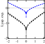
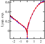
$A$		$A_{\rm fb}$

Figure 2: Lyapunov exponents $\lambda_{\rm max}$. Left: Single-layer, $N=100$, $\epsilon=1.5$ (top curve), $2.5$ (bottom curve). Right: Two-layer, $N=100$, $A_{\rm ff}=2.8,A_{1}=|A_{2}|=1$ (with $\mbox{sign}(A_{2})=\mbox{sign}(A_{\rm fb})$), $\epsilon=2.5$. Three realizations of network graphs are used in each case with their plots superimposed.

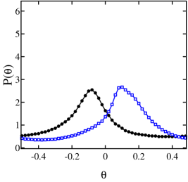
Figure 3: Phase distributions of neurons at the instant they receive an incoming spike. Left: Single-layer, $A=1.8$; all spikes. Right: Two-layer, $A_{\rm ff}=2.8$, $A_{\rm fb}=0.8$, $A_{1}=A_{2}=1$; for inter-layer spikes only – right peak for phases of Layer $1$ neurons, left peak for Layer $2$.

Fig. 2 (left) shows the basic relationship between $\lambda_{\rm max},A$, and $\epsilon$ (stimulus amplitude). Plots for $1.5<\epsilon<2.5$ interpolate between the two curves in a straightforward way. When $A=0$, i.e., when the oscillators are uncoupled, we have $\lambda_{\rm max}<0$ as expected. When $A\neq 0$, $\lambda_{\rm max}$ can be positive or negative. Notice that (i) it increases with $|A|$ for fixed $\epsilon$ (the sign of $A$ matters little), and (ii) it decreases with $\epsilon$ for fixed $A$. Item (ii) is due to the entraining effects of the stimulus; (i) suggests that the couplings here are intrinsically destabilizing. We find the value of $\lambda_{\rm max}$ to depend strongly on $A$, but only weakly on the underlying balance of $N$, $\kappa$, and $a$ for large $N$. Moreover, $\lambda_{\rm max}$ varies little among specific choices of connection graph consistent with a given $\kappa$.

At first sight, the single-layer network may appear unexpectedly reliable: At $A=2$, each neuron is expected to be perturbed by $\frac{1}{3}$ of a cycle per unit time, yet Fig. 2 (left) shows $\lambda_{\rm max}$ can still be negative. This is due to the tendency of the network to synchronize, i.e., to spike at roughly the same times (see Fig. 3, left). Because $z(\theta)=z^{\prime}(\theta)=0$ when $\theta=0$, near-synchronization means that $z(\theta)$ is typically quite small when a spike arrives, so that the effective total coupling strengths are considerably smaller than the a priori strength $A$. Perfect synchrony is not possible here due to heterogeneity in the $\omega_{i}$ and $a_{ji}$. For a given network topology, greater homogeneity in $\omega_{i}$ and $a_{ji}$ will lead to greater synchrony and smaller effective coupling paper3 .

$t$

Figure 4: The bulk synaptic output function $S(t)$; one trial each for the two sets of parameters in Fig. 1.

Two-layer networks. We again express $\lambda_{\rm max}$ in terms of $A_{1}$, $A_{2}$, $A_{\rm ff}$, and $A_{\rm fb}$, defined to be $\frac{\kappa}{2}=0.1~{}N$ times $a_{1}$, $a_{2}$, $a_{\rm ff}$, and $a_{\rm fb}$, respectively. The interpretations are as before, e.g., $A_{\rm ff}$ is the a priori total kick received per unit time by each neuron in Layer 2 from neurons in Layer 1.

Fig. 2 (right) shows $\lambda_{\rm max}$ as a function of $A_{\rm fb}$ with $A_{\rm ff}=2.8$, $A_{1}=A_{2}=\pm 1$ (we give $A_{1}$ and $A_{2}$ the same signs as $A_{\rm ff}$ and $A_{\rm fb}$, respectively, as each neuron is either excitatory or inhibitory), and $\epsilon=2.5$. At $A_{\rm fb}=0$, the system is definitively reliable. As $|A_{\rm fb}|$ increases, however, we find that the network loses its reliability almost immediately, even before $|A_{\rm fb}|\approx\frac{1}{10}A_{\rm ff}$.

This rather surprising fact is also partially explained by the phase distributions of Layer 1 and Layer 2 neurons at the instants when they receive inputs from the other layer (see Fig. 3, right). The distributions are more spread out than in the single-layer case; moreover, their peaks are centered away from $\theta=0$. This can be predicted from reduced two-neuron models paper3 . Thus at the same numerical values, $A_{\rm ff}$ and $A_{\rm fb}$ in the two-layer model are significantly more destabilizing than $A$ in the single-layer model. See also feedback .

We expect the ideas above, i.e., the tendency to synchronize within each layer, and the dominant effects of inter-layer interactions, to extend to multi-layer systems.

Figure 5: Mean across-trial variances $\bar{V}$. Left: $\bar{V}/N^{2}$ as function of $N$ for $A_{\rm ff}=2.8,A_{\rm fb}=2.5$. Right: $\bar{V}$ as function of $A_{\rm fb}$. The setup is identical to that in Fig. 2 (right); $N=100$.

III. Reliability of pooled responses. Bulk measurements have arguably greater impacts than the behavior of individual neurons. A function representing the total synaptic output of a system is defined by (cf. maz ; knight )

$$S(t)=\sum f(t-T_{i})~{};\quad f(t)=\tau^{-1}e^{-t/\tau}~{},$$

where $T_{i}$ are spike times of any neuron in the network, the summation is over all $T_{i}<t$, $f$ is a postsynaptic current, and $\tau\approx\frac{1}{15}$. Pooled-response reliability describes how repeatable $S(t)$ is in response to $I(t)$. Clearly, neuronal reliability implies pooled-response reliability. On the other hand, one would expect individual neurons to be more volatile than the network as a whole.

Two time courses for $S(t)$ are shown in Fig. 4. The first is for a reliable single-layer system; tall, well-defined spikes are generated when the system is in partial synchrony. The second is for an unreliable, 2-layer model. Here the floor of $S(t)$ is strictly positive, i.e., some neurons in the system are spiking at nearly all times.

For each $t$, we measure the repeatability of $S(t)$ by its time-dependent, across-trial variance $V(t)$; this information can be distilled further to give a single number $\bar{V}$ by time averaging $V(t)$. Our main finding is that $\bar{V}/N^{2}$ decreases as $N$ gets larger; see Fig. 5 (left). Though beyond the reach of ergodic theorems, it is apparent that due to the effects of averaging, total synaptic outputs of sufficiently large networks tend to be reliable, even as individual neurons behave unreliably.

Next, we fix $N$. As parameters are varied, we find strong correlation between $\lambda_{\rm max}$ and $\bar{V}$; compare Figs. 2 (right) and 5 (right). This confirms that the two different ways of measuring unreliability we have proposed are in good qualitative agreement.

IV. Effects of noise. By “noise”, we refer to trial-to-trial fluctuations not modeled by Eq. (1). For a clear conceptual understanding of its impact on reliability, we find it useful to distinguish between (i) noise that affects each neuron differently (e.g. synaptic or membrane noise), and (ii) noise that affects the entire population in essentially the same way (e.g., noise associated with the stimulus $I(t)$) maz ; noise . As an idealization, we add to Eq. (1) two noise terms:

$$\dot{\theta}_{i}=\omega_{i}+z(\theta_{i})\cdot\Big{[}\sum_{j\neq i}a_{ji}\ g(\theta_{j})+\epsilon_{i}I(t)+\sigma_{\ell}\eta_{i}(t)+\sigma_{g}\zeta(t)\Big{]}$$

Here $\zeta(t)$ and $\eta_{i}(t)$ are white noise realizations which vary independently from trial to trial; additionally, the $\eta_{i}(t)$ are independent for each $i$. We refer to $\eta_{i}(t)$ and $\zeta(t)$ as “local” and “global” noise; their respective amplitudes are denoted by $\sigma_{\ell}$ and $\sigma_{g}$.

Our simulations show that neuronal reliability persists under some level of local and global noise (although a gradual degradation of spike time precision from trial to trial is unavoidable). As expected, pooled responses can tolerate higher-amplitude noise terms.

Since local noise is more varied, one might expect it to lead to greater unreliability. This, however, is not true. We find that local noise has only a limited effect on pooled-response reliability for large networks, likely due to averaging effects. In contrast, the effects of global noise can be much more severe. The table below shows $\bar{V}/N^{2}$ in two representative cases:

			Noise amp. $(\sigma_{\ell},\sigma_{g})$
			(0, 0)	(0.3, 0)	(0, 0.3)
Case 1: Reliable			0.0	0.016	0.37
Case 2: Unreliable			0.090	0.076	0.36

Cases 1 and 2 are respectively the reliable and unreliable cases in Fig. 1. The loss of reliability (in a neuronally reliable system) due to global noise can be understood as follows: Recall from Sec. II that reliability means all trajectories independent of initial condition coalesce into a “random sink” for each $t$. Within each trial, since $\zeta(t)$ is a term of the same type as $I(t)$, its presence strengthens the effects of the stimulus, leading to more robust entrainment (see Fig. 2, left). Recall, however, that $\zeta(t)$ varies from trial to trial, so the trajectories entrain to a different stimulus, and therefore coalesce to a different state on each trial. When $\sigma_{g}$ is large enough, this provides a mechanism for destroying reliability.

Conclusion: We have carried out a systematic study of stimulus-response reliability for heterogeneous, layered networks of neural oscillators. Our findings – all of which are new in the present context and are consistent with results of earlier studies of different models – are of a very basic nature and thus are likely to shed light on situations beyond those considered here:

(1) On the neuronal level, single-layer networks are fairly reliable due to a tendency to synchronize, while recurrent connections can be strongly destabilizing in two-layer systems. In general, individual neurons can behave reliably or unreliably as a result of the competition between entrainment to the stimulus or upstream layer and the perturbative effects of other synaptic events.

(2) Pooled responses of large enough networks are mostly reliable even when individual neurons within it are not. In a fixed-size network, they have similar reliability properties as individual neurons but with lower volatility.

(3) Global noise, i.e., noise that affects the entire population in roughly the same way, can seriously jeopardize even pooled-response reliability, while local noise has only limited effect.

E.S-B. is supported by a Burroughs-Wellcome Fund Career Award; L-S.Y. is supported by a grant from the NSF. The authors thank D. Cai and J. Rinzel for helpful discussions.

References

- (1) F. Rieke et al., Spikes (MIT Press, 1996); D. Perkel & T. Bullock, Neurosci. Res. Program Bull. 6 221 (1968).
- (2) H. Bryant & J. Segundo, J. Physiol. 260 279 (1976); Z. Mainen & T. Sejnowski, Science 268 1503 (1995).
- (3) J. Teramae & D. Tanaka, Phys. Rev. Lett. 93 204103 (2004); J. Ritt, Phys. Rev. E 68 041915 (2003).
- (4) H. Nakao et al., Phys. Rev. E 72 026220 (2005); C. Zhou & J. Kurths, Chaos 13 401 (2003); K. Pakdaman & D. Mestivier, Phys. Rev. E 64 030901 (2001); A. Pikovsky, M. Rosenblum, & J. Kurths, Synchronization (Cambridge U. Press, 2001).
- (5) K. K. Lin & E. Shea-Brown & L.-S. Young, aXiv nlin.CD/0708.3061; ibid. 0708.3063.
- (6) C. van Vreeswijk, C. & H. Sompolinsky, Science 274 1724 (1996); A. Banerjee, J. Comp. Neurosci. 20 321 (2006); M. Bazhenov et al, Phys. Rev. E 72 041903 (2005).
- (7) J. Teramae & T. Fukai, arXiv nlin.CD/0708.0862
- (8) M.Berry, D.Warland, M.Meister, PNAS 94 5411 (1997); G. Murphy, F. Rieke, Neuron 52 511 (2006); R. de Ruyter van Steveninck et al., Science 275 1805 (1997);P. Kara, P. Reinagel, R. Reid, Neuron 27 635 (2000).
- (9) G. Shepard, The Synaptic Organization of the Brain, Oxford Univ. Press, 2004; E. Douglas & K. Martin, Annu. Rev. Neurosci. 27 (2004).
- (10) A. Winfree, Geometry of Bio. Time (Springer, 2001)
- (11) G.B. Ermentrout, Neural Comp. 8 979 (1996).
- (12) Specifically, we set for .
- (13) L. Arnold, Random Dyn. Sys., (Springer, 2003); P. H. Baxendale, Progr. Probab. 27 (Birkhäuser, 1992).
- (14) Y. Le Jan, Z. Wahr. Verw. Geb. 70 (1985); F. Ledrappier & L.-S. Young, Probab. Th. & Rel. Fields 80 217 (1988).
- (15) We compute by solving the variational equation for the SDE (1) using the Milstein scheme.
- (16) K. K. Lin, E. Shea-Brown, & L.-S. Young. In preparation.
- (17) Y. Aviel, C. Mehring, M. Abeles, & D. Horn, Neural Comp. 15 (2003); V. Litvak, H. Sompolinsky, I. Segev, & M. Abeles, J. Neurosci 23 (2003); T. P. Vogels & L. F. Abbott, J. Neurosci 25 (2005).
- (18) M. Mazurek & M. Shadlen, Nat. Neursci. 5 463 (2002); M. Shadlen & W. Newsome, J. Neurosci. 18 3870 (1998).
- (19) B. Knight, Neural Comp. 12 473 (2000).
- (20) A. A. Faisal, L. P. J. Selen, & D. M. Wolpert, Nat. Rev. Neurosci. 9 (2008).