Non-equilibrium of Ionization and the Detection of Hot Plasma in Nanoflare-heated Coronal Loops
Abstract
Impulsive nanoflares are expected to transiently heat the plasma confined in coronal loops to temperatures of the order of 10 MK. Such hot plasma is hardly detected in quiet and active regions, outside flares. During rapid and short heat pulses in rarified loops the plasma can be highly out of equilibrium of ionization. Here we investigate the effects of the non-equilibrium of ionization (NEI) on the detection of hot plasma in coronal loops. Time-dependent loop hydrodynamic simulations are specifically devoted to this task, including saturated thermal conduction, and coupled to the detailed solution of the equations of ionization rate for several abundant elements. In our simulations, initially cool and rarified magnetic flux tubes are heated to 10 MK by nanoflares deposited either at the footpoints or at the loop apex. We test for different pulse durations, and find that, due to NEI effects, the loop plasma may never be detected at temperatures above MK for heat pulses shorter than about 1 min. We discuss some implications in the framework of multi-stranded nanoflare-heated coronal loops.
1 Introduction
Nanoflares – small scale highly transient heating episodes – are among the main candidates as source of coronal loop heating (e.g., Parker 1988; Cargill 1994; Klimchuk 2006 and references therein). The conjecture is still under debate because nanoflares have been hardly detected so far. There are many possible reasons for this difficult detection. For instance, a very frequent occurrence may inhibit the resolution of the single event. Also the efficient thermal conduction and low emission measure during the pulses can reduce and delay the signatures of the heating (e.g., Peres et al. 1987; Reale & Peres 1995). Also very small pulses distributed in a very finely structured loop may be difficult to detect. One of the main arguments invoked as crucial evidence of nanoflare heating is the detection of high temperature ( MK) plasma components in observations of coronal loops (Cargill & Klimchuk 1997; Klimchuk 2006), outside of proper flares. The presence of such hot component is often predicted by hydrodynamic modeling of coronal loops heated by transient pulses (Patsourakos & Klimchuk 2005; Patsourakos & Klimchuk 2006; Cargill & Klimchuk 2004). In particular any heat spike able to bring the loop to the observed brightness should be so intense as to heat the plasma to temperatures of the order of MK at least for a transient time interval. In the hypothesis of a finely structured loop where a whole distribution of heat pulses occur continuously, such plasma might be detectable, at least as a hot tail in the emission measure distribution. The evidence of hot plasma has been difficult so far. For instance, a dominant plasma component at about 3 MK is shown by recent thermal maps of active regions obtained from wide-band multi-filter imaging observations (Reale et al. 2007) with the X-Ray Telescope (XRT, Golub et al. 2007) on board the Hinode mission (Kosugi et al. 2007).
There are possible explanations also for the difficult detection of hot plasma. The most immediate one is linked to the inertia of the plasma dynamics. A heat pulse deposited in a coronal loop drives evaporation of chromospheric plasma. The loop is filled with hot and dense plasma which makes it bright in the X-rays. For short heat pulses, the plasma may evaporate from the chromosphere on time scales longer than the heat duration. Therefore the heated strand may only later acquire enough emission measure to become visible, while it is cooling. However, in short loops ( cm) the sound crossing time is of the order of one minute (e.g., Reale 2007) and we may expect to detect hot spots within less than half a minute.
There is another less obvious effect which may make the detection of hot plasma harder: the time lag of the plasma to change its ionization from a cool to a hot state. An impulsive energy input drives plasma thermal and dynamic changes on relatively short timescales. Electron excitation, de-excitation, ionization and recombination processes of the ion species have other timescales. If the timescale, for instance, of the temperature evolution is much shorter than the ionization and recombination timescales, the degree of ionization can be very different from the equilibrium conditions corresponding to the local electron temperature (Shapiro & Moore 1977; Orlando et al. 1999; Klimchuk 2006). So, during a fast temperature increase, the plasma ions can be at a lower ionization state than the equilibrium state corresponding to the instantaneous temperature. Such non-equilibrium of ionization (NEI) effects may become important in the interpretation of what we observe. If the heat pulse is sufficiently short, the ions and their emitted radiation may not even have enough time to “sense” the hot temperature status, they would adjust to the temperature variations deep in the cooling phase, and we would detect radiation from cooler ion conditions at any time.
NEI effects in nanoflare-heated loops have already been investigated in the past. Mariska et al. (1982) found that NEI can significantly alter the relative ionic abundances in the quiet corona. Golub et al. (1989) examine the effect of NEI on the observability of coronal variations. Bradshaw & Mason (2003) found that NEI can modify considerably the radiative losses function. Müller et al. (2003) investigated the role of NEI in the transition region brightenings driven by loop condensations. Bradshaw & Cargill (2006) model nanoflare heating in coronal loops and remark the importance of NEI effects, the presence of hot plasma with low emission measure, and Doppler-shifts as possible diagnostics of the heating.
Here we investigate the effect of NEI during nanoflaring activity on the detectability of hot plasma in coronal loops. We will model a coronal loop strand heated by nanoflares of different durations, compute the corresponding evolution of the relevant ion species, and compare it with the evolution in full ionization equilibrium. We will evaluate the effects on the expected temperature distribution of the loop emission measure, which will tell us about the existence of significantly emitting hot plasma components. This will allow us to put constraints on the nanoflare characteristics which lead to the observability of hot plasma and indirectly also on the fine loop structuring. In Sec.2 the modeling is described, in Sec.3 the results are illustrated and discussed in Sec.4.
2 Modeling
Our model is set up to explore the conditions for plasma confined in a coronal magnetic flux tube and heated to MK by nanoflares to be detectable as hot plasma considering the effects of NEI. The coronal loop contains low plasma, and, as customary for standard loop models, we assume that plasma moves and transports energy only along the magnetic field lines, so that a one-dimensional description is adequate (e.g., Peres et al. 1982). The model takes into account the gravity stratification, the thermal conduction (including the effects of heat flux saturation), the radiative losses, an external heating input, and the NEI effects. The following fluid equations of mass, momentum, and energy conservation are solved, considering only the relevant components along the loop magnetic field lines:
| (1) |
| (2) |
| (3) | |||||
is the total gas energy (internal energy, , and kinetic energy), is the time, is the coordinate along the loop, is the mass density, is the mean atomic mass (assuming solar abundances), is the mass of the hydrogen atom, is the hydrogen number density, is the electron number density, v the plasma flow speed, the pressure, g the gravity, the temperature, the conductive flux, a function describing the transient input heating, is the radiative losses per unit emission measure (e.g. Raymond & Smith 1977; Mewe et al. 1985; Kaastra & Mewe 2000). Here we consider the radiative losses function in equilibrium of ionization. Although this assumption makes our description not entirely self-consistent, it does not affect significantly our results, because in the critical evolution phases the energy losses are dominated by transport by thermal conduction (see Sec.3.1). We use the ideal gas law, , where is the ratio of specific heats.
The set of the continuity equations for each ion species is expressed as:
| (4) |
is the number density of the -th ion of the element , is the number of elements, the number of ionization states of element , are the collisional and dielectronic recombination coefficients, and the collisional ionization coefficients (Summers 1974).
Given the importance of rapid transients, fast dynamics and steep thermal gradients in this work, we consider both the classical and saturated conduction regimes. To allow for a smooth transition between them, we follow Dalton & Balbus (1993) and define the conductive flux as
| (5) |
Here represents the classical conductive flux (Spitzer 1962)
| (6) |
where the thermal conductivity is erg s-1 K-1 cm-1. The saturated flux, , is (Cowie & McKee 1977)
| (7) |
where is the isothermal sound speed, and is a correction factor of the order of unity. We set according to the values suggested for the coronal plasma (Giuliani 1984; Borkowski et al. 1989, Fadeyev et al. 2002, and references therein).
The transient input heating is described empirically as a separate function of space and time:
| (8) |
where is a Gaussian function:
| (9) |
and is a pulse function:
| (10) |
The calculations described in this paper were performed using the 1-D version of the flash code (Fryxell et al. 2000), an adaptive mesh refinement multiphysics code. For the present application, the code has been extended by additional computational modules to handle the plasma thermal conduction (see Orlando et al. 2005 for details of the implementation), the NEI effects, the radiative losses, and the heating function. The implementation of the description of the ionization balance in the flash code is described in the Appendix.
We consider an initially cool and rarified semicircular magnetic flux tube (loop or loop strand) with half-length cm, and uniform cross-section area. The area appears only as a multiplicative factor in this description and the size is typical of active region loops. The loop is initially at equilibrium according to loop scaling laws (Rosner et al. 1978) and to hydrostatic conditions (Serio et al. 1981) assuming it lies on a plane vertical to the solar surface. The initial base pressure is dyn/cm2, corresponding to a maximum temperature MK, at the loop apex. The corona is linked with a steep transition region to an isothermal chromosphere uniformly at K and cm thick. We assume that the loop is symmetric with respect to the vertical axis across the apex, and therefore we simulate only half of the loop, with a total extension of cm. All the ion species are assumed initially in equilibrium of ionization in the whole computational domain.
At the coarsest resolution, the adaptive mesh algorithm used in the flash code (paramesh; MacNeice et al. 2000) uniformly covers the computational domain with a mesh of blocks, each with cells. We allow for 3 levels of refinement, with resolution increasing twice at each refinement level. The refinement criterion adopted (Löhner 1987) follows the changes in density and temperature. This grid configuration yields an effective resolution of cm at the finest level, corresponding to an equivalent uniform mesh of grid points. We use fixed boundary conditions at and reflecting boundary conditions at (consistent with the adopted symmetry).
3 Results
3.1 The Simulations
In the loop outlined above we inject one nanoflare as intense as to heat the plasma and keep it at MK, if the heating were steady. The choice of the parameters is dictated by our scope of exploring the influence of NEI on the detectable thermal conditions. In this perspective, the pulse duration becomes the critical parameter: if the heat pulse is short enough, the plasma may not have enough time to adjust to ionization conditions appropriate of 10 MK, before the heating is off. Therefore, we consider longer and longer heat pulse durations with a logarithmic sampling, i.e. s, 30 s, 180 s. For each of these durations we consider two possible locations of the pulse depositions: at the footpoints, namely cm from the base of the chromosphere (i.e. cm from the base of the corona) and at the apex, namely cm. The spatial width of the pulse is smaller at the footpoints ( cm) and larger at the apex ( cm). To have the same total energy deposition rate, the maximum volume deposition rates are erg cm-3 s-1 and erg cm-3 s-1, respectively.
We come out with a total of six simulations. They are carried out for a time which covers the pulse duration and a couple of loop cooling times:
| (11) |
where is in units of cm and is the loop maximum temperature in units of MK (Serio et al. 1991). All simulations then span a time interval of about 800 s.
The evolution of nanoflaring plasma confined in coronal loops is well-known from previous work (Peres et al. 1993;Warren et al. 2002;Warren et al. 2003;Patsourakos & Klimchuk 2005;Testa et al. 2005) and is on a smaller scale similar to that of properly flaring loops (e.g. Nagai 1980;Peres et al. 1982;Doschek et al. 1983;Nagai & Emslie 1984;Fisher et al. 1985;Peres et al. 1987;Reale & Peres 1995). As additional feature, our simulations include the effect of saturated thermal conduction, which might be important here since we study the evolution on small time scales (see also Klimchuk et al. 2003). In the following, we just draw a basic outline of the results adapted to our simulations.
Let’s consider the simulation with s and heat pulses deposited at the footpoints (Fig. 1). The sudden heat deposition determines a local increase of temperature (to MK) and pressure (to dyn/cm2). A fast thermal front propagates upwards along the loop. The cool chromosphere is heated and expands upwards with a strong evaporation front. By the time the thermal front has reached cm and the evaporation front cm, the heat pulse is already over. Due to efficient thermal conduction, the plasma then immediately begins to cool, already during the propagation of the thermal front, and the maximum temperature rapidly decreases to MK in less than a minute. The thermal front reaches the apex, and therefore the loop thermalizes, in s. The impulsive evaporation front moves at velocity of about 300 km/s (Fig.3D) and fills the loop in s. The density keeps on increasing throughout the loop with more gentle fronts (the peak velocity rapidly decreases to less than 200 km/s) for further tens of seconds. Meanwhile the plasma accumulates at the apex reaching a density of about cm-3. The compression heats the plasma again above 3 MK at the apex. Then the plasma begins to drain and the density to decrease (not shown), following the radiation cooling time (Cargill & Klimchuk 2004; Reale 2007).

The overall evolution does not change much in the other simulations. Longer heat pulses drive more and longer plasma evaporation. Pulses deposited at the apex produce downward thermal fronts but as soon as the thermal front hits the chromosphere, it drives an evaporation front similar to that driven by the pulses at the footpoints.
3.2 Non-equilibrium of Ionization
The importance of highly transient processes such as NEI is basically dictated by their timescales related to the timescales of the dynamics and heating/cooling driven by the nanoflares. Fig. 2 shows the combined ionization/recombination timescale for the i-th ion species of the element , derived from Eq.(4) as
| (12) |
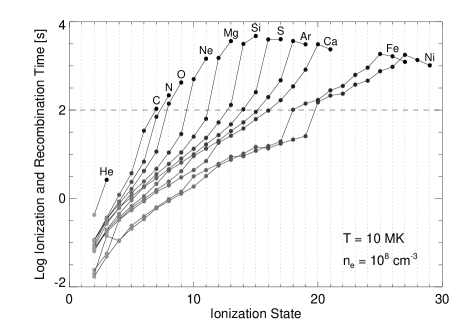
for twelve important elements, computed for a temperature MK and a density cm-3. Analogous timescales have been provided, in tabular form, by Golub et al. (1989) in the study of observable variability of spectral lines in soft X-ray and XUV regions of the solar corona.
Clearly, increases with the ion species and becomes larger than 100 s for the highest ion species of C, N, O, Ne, Mg, Si, S, Ar and Ca. More species are involved in high ionization times for Fe and Ni. The modeling shows that the plasma immediately cools down considerably as soon as the heat pulse stops. As a consequence, from Fig. 2 we expect that the high ion species will have no time to adjust to high temperature status if the heat pulse lasts significantly less than 100 s.
The ionization and recombination timescale is dominated by either ionization or recombination rate, depending on the sign of the temperature jump and on the ionization state of the element considered: in general, is dominated by the ionization rate for the lowest ion species and by the recombination rate for the highest ion species. The ionization state for which ionization and recombination rates are comparable depends on the temperature: the higher the temperature, the higher is this ionization state. In the case considered here, is dominated by the ionization rate for most of the ion populations (see also Patsourakos & Klimchuk 2006) and by recombination rate for the top ionization states (e.g. Si XV, S XVI, Ca 20, Fe XXVI). As shown later, we found the effective ionization temperature generally lower than the electron temperature, even when the plasma is cooling; as a consequence, in the case of nanoflares discussed here, is generally dominated by the ionization rate for most of the ion populations.
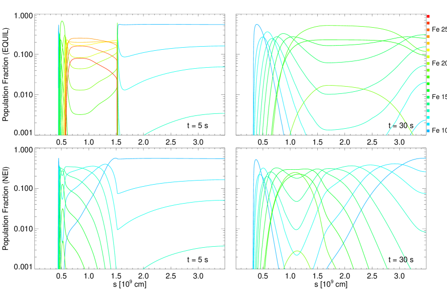
As an example, Fig. 3 shows the distribution of population fractions of Fe along the loop derived assuming equilibrium ionization (upper panels) and considering the deviations from equilibrium ionization (lower panels) for the simulation with heat pulses deposited at the footpoints lasting s (see also Fig. 1). During the early phase of the evolution, the deviations from equilibrium of ionization are very large at the loop footpoints due to the sudden local increase of temperature to MK (see left panels of Fig. 3). Whereas significant populations are expected above Fe XX low in the loop (below cm, reddish lines in the upper left panel), no such highly ionized Fe species appears when NEI is taken into account. As expected, the high ion species are not able to adjust to the plasma temperature before the heat pulse is over. Then the plasma cools down reducing the deviations from equilibrium ionization. The deviations are still significant later at s, when the loop has thermalized (see Fig. 1) and the maximum temperature is MK. At this time, no highly ionized Fe species is present both considering and not considering NEI, because of the effective cooling.
This time lag of the evolution of the ion species has important implications on the temperature diagnostics of the plasma from its emission. To address this issue, from the modeled population fractions, we derive the temperature which best matches the actual ionization state of the ion species for each of the elements in our simulations: operatively this is found as the one of the equilibrium temperatures with the most similar three most populated ionized states. It is worth noting that at least two population fractions are necessary to find a unique value of temperature and that this “NEI” temperature should not be intended as an exact temperature but as the temperature which best describes the ionization state. This is done at each time and position along the loop. Fig. 4 shows the evolution (on a logarithmic time scale) of the plasma maximum temperature and of the maximum NEI temperature for five representative elements (C, O, Mg, S, Fe). In the same figure the evolution of the coronal emission measure at the maximum plasma temperature is also shown for comparison. The ion species adjust to a hotter status very gradually, on a time scale of about 100 s (Fig. 2). Since this time is slightly longer than the time taken by the emission measure to increase significantly (as shown by the bottom panels), we expect observable effects in the X-ray band. For s, despite the maximum electron temperature is above 10 MK, all the ion species are never represented by a temperature larger than about 3 MK all over the event, for any pulse location. For s, Fe (and Ni) reaches a temperature about MK for pulses located at the footpoints and about 6 MK for pulse deposited at the apex. This occurs for a very limited time range (between 100 and 200 s). The other elements mostly stay at temperatures well below 5 MK. The results change quite substantially for s. Although with delay ( s), here many elements have enough time to adjust to ionization stages typical of higher temperatures, between 7 MK and 10 MK, for both heat pulse locations. The high ionization state is maintained for longer time intervals (more than 200 s).

The effect of long-lasting NEI is illustrated synthetically in Figs. 5-7 which shows the total loop emission measure distribution with temperature, EM(), averaged over different time intervals. The figure compares EM() obtained either taking or not taking the deviations from equilibrium ionization into account; the former is obtained using the average “NEI” temperature among those of all the elements considered, the latter using directly the electron temperature.
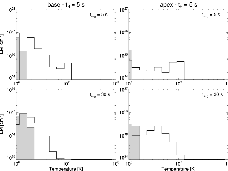
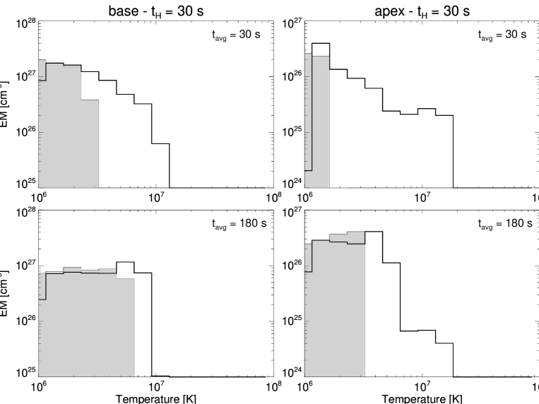
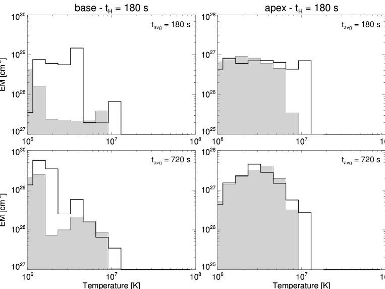
Averaging over the heat pulse duration only, we can see that EM() with and without NEI are invariably very different. The shorter the pulse duration, the more the hot components are missing from the NEI EM() distributions. For the hottest components including NEI are only at about 1 MK, which increases to 3 MK for s. The difference is less considerable for s, but even in this case the hot components are hardly above 5 MK, against 10 MK without NEI. The differences are unsurprisingly reduced when we average over longer times, which should approach a situation closer to the realistic observations. Over a few durations of the heat pulses the differences are still significant for the shortest heat pulses: for s, with NEI we do not find components above 2 MK, whereas without NEI there are components almost to 10 MK. For s the two EM() distributions are more similar, but with NEI we do not find components hotter than 6 MK. For the longest pulse duration, the EM(T) distributions almost coincide.
4 Discussion and conclusions
The target of this work is to explore the effect of non-equilibrium of ionization (NEI) in nanoflare-heated loops. The importance of NEI effects on coronal observations had been already pointed out and evaluated by Golub et al. (1989). That study was devoted more specifically to the diagnostics of rapid variability. Here, we focus on the effects on the detection of hot plasma in nano-flaring loops. To this purpose we set up hydrodynamic simulations of plasma confined in an active region loop heated to MK by more or less long nanoflares. As new achievements specifically set up for this study, we have included the effect of the saturated thermal conduction in the modeling (Klimchuk et al. 2003), and computed the evolution of the ion population fractions of several important elements driven by a short heat pulse. Each ion species takes a characteristic time to reach equilibrium conditions for a certain plasma temperature and density. If the plasma conditions vary on very small time scales, the ions are unable to adjust to the new and rapidly changing conditions and the emitted spectrum during the plasma variations can become very different from the one expected in equilibrium conditions. If the variation is a sudden heating followed by a sudden cooling, the emission may never or only partially adapt to the transient hot conditions. To evaluate the importance of this effect and its dependence on the heat pulse parameters, we have computed the actual temperature of the plasma as it would appear in the radiation spectrum according to the effective ionization state.
We find that the effects are significant if the heat pulses last less than a minute or so. For durations of a few seconds the spectra will never show temperatures higher than 2-3 MK even though the electron temperature overcomes 10 MK. This effect is little dependent on the location of the heat pulse, except for details. These results can be considered valid in wide generality in spite of some limitations of our approach. Our assumption of pulses leading to 10 MK is, of course, arbitrary, although this has been taken as possible typical temperature in other works (Patsourakos & Klimchuk 2006). Conclusions are certainly valid for less intense pulses, which heat less the plasma. We do not expect dramatic differences also for more intense pulses (e.g. 20 MK), because the thermal conduction becomes even more efficient and the plasma initial cooling (after the end of the pulse) will be faster. Also the details of the shape of the heat pulse should not have much influence, provided that the overall duration is the same. In general, of course, more gentle heating should make plasma reach equilibrium conditions more easily, while the opposite occurs for more spiky pulses. More important is instead our assumption of a single pulse inside a given thread. With it, we are excluding a repetition of the pulse inside the same thread, or, at least, a very long repetition time, so long as to have a rarified loop ( cm-3) again before the new ignition. More frequent pulses would be released in a denser plasma which is faster to adjust to ionization equilibrium, and in which, therefore, we expect less NEI effects. The ionization times in fact scale inversely with plasma density. Heat pulses released in a cm-3 dense plasma, i.e. about ten times denser than our initially rarified flux tube, would excite highly ionized element species about ten times more rapidly, with typical times of about ten seconds (Fig. 2).
In the range MK the plasma emits radiation mostly in the X-ray band and the spectra are dominated by the emission lines produced by the recombination and deexcitation of highly ionized atoms (e.g., Tucker & Koren 1971, Kato 1976). For instance, hundreds of lines of at least ten Fe ion species populate the spectra of plasma in that range of temperature. For this reason, the ionization status of the emitting ions becomes extremely important in the thermal “appearance” of the plasma, which we detect through its radiation with remote sensing, while the continuum electron bremsstrahlung emission – which adjusts immediately to thermal and dynamic plasma variations – becomes more important at much higher temperatures. Our results therefore apply both to the analysis of single lines through high resolution spectroscopy, and to the diagnostics from wideband multi-filter instruments in the X-ray and EUV bands, e.g. Hinode/XRT or the Atmospheric Imaging Assembly (AIA) on board the forthcoming Solar Dynamic Observatory.
According to these considerations, a hard detection of hot plasma may point to a scenario of coronal loops heated by single short and relatively intense nanoflares. Very short durations and very long repetition times naturally imply that the pulses should be deposited always in different strands and that, therefore, the strands involved should be a very large number, i.e. the loop must have a very fine transversal structure. A scenario of loops heated by short nanoflares has some important implications. Hot plasma may be difficult to detect not because of a limitation of the telescopes, detectors and filters, but due to an intrinsic property of the plasma emission. The critical parameter for detectability of hot plasma is the duration of the heat pulse and minute is the critical duration value, a useful indication for detailed models of nanoflaring mechanisms. The fine temporal structure would also automatically imply a very fine spatial structure, difficult to resolve.
This picture is fully compatible with the current scenario of nanoflaring multi-stranded coronal loops. For instance, it naturally involves the hot-underdense/cool-overdense loop cycle (Warren et al. 2002,Cargill & Klimchuk 2004, Klimchuk 2006). Less trivial is the effect on the diagnostics of the detailed thermal structure along and across the loops (e.g., Cargill & Klimchuk 2004, Aschwanden & Nightingale 2005, Reale & Ciaravella 2006, Schmelz et al. 2007), which we defer to later work.
In conclusion, we have investigated in detail the effect of the non-equilibrium of ionization driven by nanoflares in finely structured coronal loops on the detection of hot plasma in the loops, and provided constraints on the heat pulse duration which may make or make not the detection difficult. Further more detailed information and diagnostics are expected from high resolution spectroscopy such as that from EUV Imaging Spectrometer on board the Hinode mission or from the Extreme Ultraviolet Variablity Experiment (EVE) on board the forthcoming Solar Dynamic Observatory.
Appendix A Non-equilibrium ionization in the FLASH code
The non-equilibrium ionization is added to the FLASH code using a method of time splitting between the hydrodynamic and the NEI numerical modules. A fractional step method is required to integrate the equations and in particular to decouple the NEI solver from the hydrodynamic solver. For each timestep, the homogeneous hydrodynamic transport equations given by Eqs. 1–4 are solved using the FLASH hydrodynamic solver with R = 0. After each transport step, the stiff system of ordinary differential equations for the NEI problem with the form:
| (A1) |
are integrated. This step incorporates the reactive source terms. Within each grid cell, the above equations can be solved separately with a standard ODE method. Since this system is stiff, it is solved using the Bader-Deuflhard time integration solver111The variable-order Bader-Deuflhard routine used here is a combination of the routine METANI given by Bader & Deuflhard (1983) and the routine STIFBS given by Press et al. (1996) (see also Timmes 1999). with the MA28 sparse matrix package. Timmes (1999) has shown that these two algorithms together provide the best balance of accuracy and overall efficiency. Note that the source term in the NEI module is adequate to solve the problem for optically thin plasma in the coronal approximation; just collisional ionization, auto-ionization, radiative recombination, and dielectronic recombination are considered.
References
- Aschwanden & Nightingale (2005) Aschwanden, M. J., & Nightingale, R. W. 2005, ApJ, 633, 499
- Bader & Deuflhard (1983) Bader, G., & Deuflhard, P. 1983, Numer. Math., 41, 373
- Borkowski et al. (1989) Borkowski, K. J., Shull, J. M., & McKee, C. F. 1989, ApJ, 336, 979
- Bradshaw & Cargill (2006) Bradshaw, S. J., & Cargill, P. J. 2006, A&A, 458, 987
- Bradshaw & Mason (2003) Bradshaw, S. J., & Mason, H. E. 2003, A&A, 407, 1127
- Cargill (1994) Cargill, P. J. 1994, ApJ, 422, 381
- Cargill & Klimchuk (1997) Cargill, P. J., & Klimchuk, J. A. 1997, ApJ, 478, 799
- Cargill & Klimchuk (2004) —. 2004, ApJ, 605, 911
- Cowie & McKee (1977) Cowie, L. L., & McKee, C. F. 1977, ApJ, 211, 135
- Dalton & Balbus (1993) Dalton, W. W., & Balbus, S. A. 1993, ApJ, 404, 625
- Doschek et al. (1983) Doschek, G. A., Cheng, C. C., Oran, E. S., Boris, J. P., & Mariska, J. T. 1983, ApJ, 265, 1103
- Fadeyev et al. (2002) Fadeyev, Y. A., Le Coroller, H., & Gillet, D. 2002, A&A, 392, 735
- Fisher et al. (1985) Fisher, G. H., Canfield, R. C., & McClymont, A. N. 1985, ApJ, 289, 414
- Fryxell et al. (2000) Fryxell, B. et al. 2000, ApJS, 131, 273
- Giuliani (1984) Giuliani, J. L. 1984, ApJ, 277, 605
- Golub et al. (2007) Golub, L. et al. 2007, Sol. Phys., 243, 63
- Golub et al. (1989) Golub, L., Hartquist, T. W., & Quillen, A. C. 1989, Sol. Phys., 122, 245
- Kaastra & Mewe (2000) Kaastra, J. S., & Mewe, R. 2000, in Atomic Data Needs for X-ray Astronomy, p. 161
- Kato (1976) Kato, T. 1976, ApJS, 30, 397
- Klimchuk (2006) Klimchuk, J. A. 2006, Sol. Phys., 234, 41
- Klimchuk et al. (2003) Klimchuk, J. A., Patsourakos, S., & Winebarger, A. R. 2003, in Bulletin of the American Astronomical Society, Vol. 35, Bulletin of the American Astronomical Society, 825–+
- Kosugi et al. (2007) Kosugi, T. et al. 2007, Sol. Phys., 243, 3
- Löhner (1987) Löhner, R. 1987, Comp. Meth. Appl. Mech. Eng., 61, 323
- MacNeice et al. (2000) MacNeice, P., Olson, K. M., Mobarry, C., de Fainchtein, R., & Packer, C. 2000, Comp. Phys. Comm., 126, 330
- Mariska et al. (1982) Mariska, J. T., Doschek, G. A., Boris, J. P., Oran, E. S., & Young, Jr., T. R. 1982, ApJ, 255, 783
- Mewe et al. (1985) Mewe, R., Gronenschild, E. H. B. M., & van den Oord, G. H. J. 1985, A&AS, 62, 197
- Müller et al. (2003) Müller, D. A. N., Hansteen, V. H., & Peter, H. 2003, A&A, 411, 605
- Nagai (1980) Nagai, F. 1980, Sol. Phys., 68, 351
- Nagai & Emslie (1984) Nagai, F., & Emslie, A. G. 1984, ApJ, 279, 896
- Orlando et al. (1999) Orlando, S., Bocchino, F., & Peres, G. 1999, A&A, 346, 1003
- Orlando et al. (2005) Orlando, S., Peres, G., Reale, F., Bocchino, F., Rosner, R., Plewa, T., & Siegel, A. 2005, A&A, 444, 505
- Parker (1988) Parker, E. N. 1988, ApJ, 330, 474
- Patsourakos & Klimchuk (2005) Patsourakos, S., & Klimchuk, J. A. 2005, ApJ, 628, 1023
- Patsourakos & Klimchuk (2006) —. 2006, ApJ, 647, 1452
- Peres et al. (1993) Peres, G., Reale, F., & Serio, S. 1993, in Physics of Solar and Stellar Coronae: G. S. Vaiana Memorial Symposium, held 22-26 June, 1992, in Palermo, Italy. Edited by Jeffrey L. Linsky and Salvatore Serio. Astrophysics and Space Science Library, Vol. 183. Published by Kluwer Academoc Publishers, P. O. Box 17, 3300 AA Dordrecht, The Netherlands, 1993., p.151, ed. J. L. Linsky & S. Serio, 151–+
- Peres et al. (1987) Peres, G., Reale, F., Serio, S., & Pallavicini, R. 1987, ApJ, 312, 895
- Peres et al. (1982) Peres, G., Serio, S., Vaiana, G. S., & Rosner, R. 1982, ApJ, 252, 791
- Press et al. (1996) Press, W. H., Teukolsky, S. A., Vetterling, W. T., & Flannery, B. P. 1996, Numerical recipes in FORTRAN 90 (Cambridge: University Press)
- Raymond & Smith (1977) Raymond, J. C., & Smith, B. W. 1977, ApJS, 35, 419
- Reale (2007) Reale, F. 2007, A&A, 471, 271
- Reale & Ciaravella (2006) Reale, F., & Ciaravella, A. 2006, A&A, 449, 1177
- Reale et al. (2007) Reale, F. et al. 2007, Science, 318, 1582
- Reale & Peres (1995) Reale, F., & Peres, G. 1995, A&A, 299, 225
- Rosner et al. (1978) Rosner, R., Tucker, W. H., & Vaiana, G. S. 1978, ApJ, 220, 643
- Schmelz et al. (2007) Schmelz, J. T., Nasraoui, K., Del Zanna, G., Cirtain, J. W., DeLuca, E. E., & Mason, H. E. 2007, ApJ, 658, L119
- Serio et al. (1981) Serio, S., Peres, G., Vaiana, G. S., Golub, L., & Rosner, R. 1981, ApJ, 243, 288
- Serio et al. (1991) Serio, S., Reale, F., Jakimiec, J., Sylwester, B., & Sylwester, J. 1991, A&A, 241, 197
- Shapiro & Moore (1977) Shapiro, P. R., & Moore, R. T. 1977, ApJ, 217, 621
- Spitzer (1962) Spitzer, L. 1962, Physics of Fully Ionized Gases (New York: Interscience, 1962)
- Summers (1974) Summers, H. P. 1974, Internal Mem., Vol. 367 (Astrophysics Research Div., Appleton Lab., Abingdon, Oxon)
- Testa et al. (2005) Testa, P., Peres, G., & Reale, F. 2005, ApJ, 622, 695
- Timmes (1999) Timmes, F. X. 1999, ApJS, 124, 241
- Tucker & Koren (1971) Tucker, W. H., & Koren, M. 1971, ApJ, 168, 283
- Warren et al. (2002) Warren, H. P., Winebarger, A. R., & Hamilton, P. S. 2002, ApJ, 579, L41
- Warren et al. (2003) Warren, H. P., Winebarger, A. R., & Mariska, J. T. 2003, ApJ, 593, 1174