$S$–pairing in neutron matter
I. Correlated Basis Function Theory

Adelchi Fabrocini Adelchi.Fabrocini@df.unipi.it Dipartimento di Fisica “Enrico Fermi”, Università di Pisa INFN, Sezione di Pisa, I-56100 Pisa, Italy    Stefano Fantoni fantoni@sissa.it International School for Advanced Studies, SISSA INFM DEMOCRITOS National Simulation Center, I-34014 Trieste, Italy    Alexey Yu. Illarionov illario@sissa.it International School for Advanced Studies, SISSA, I-34014 Trieste, Italy INFN, Sezione di Pisa, I-56100 Pisa, Italy    Kevin E. Schmidt Kevin.Schmidt@asu.edu Department of Physics and Astronomy, Arizona State University, Tempe, AZ, 85287 International School for Advanced Studies, SISSA, I-34014 Trieste, Italy
Abstract

$S$–wave pairing in neutron matter is studied within an extension of correlated basis function (CBF) theory to include the strong, short range spatial correlations due to realistic nuclear forces and the pairing correlations of the Bardeen, Cooper and Schrieffer (BCS) approach. The correlation operator contains central as well as tensor components. The correlated BCS scheme of Ref. Fantoni (1981), developed for simple scalar correlations, is generalized to this more realistic case. The energy of the correlated pair condensed phase of neutron matter is evaluated at the two–body order of the cluster expansion, but considering the one–body density and the corresponding energy vertex corrections at the first order of the Power Series expansion. Based on these approximations, we have derived a system of Euler equations for the correlation factors and for the BCS amplitudes, resulting in correlated non linear gap equations, formally close to the standard BCS ones. These equations have been solved for the momentum independent part of several realistic potentials (Reid, Argonne $v_{14}$ and Argonne $v_{8^{\prime}}$) to stress the role of the tensor correlations and of the many–body effects. Simple Jastrow correlations and/or the lack of the density corrections enhance the gap with respect to uncorrelated BCS, whereas it is reduced according to the strength of the tensor interaction and following the inclusion of many–body contributions.

nuclear forces, nuclear matter, nuclear cluster models, nuclear pairing, superfluidity
pacs:
02.70.Ss, 2.70.Uu, 03.75.Hh, 03.75.Kk, 03.75.Mn, 05.10.Ln, 05.30.Fk, 05.70.Fh, 21.30.-x, 21.60.-n, 21.60.Gx, 21.60.Ka, 21.65.+f, 26.60.+c, 67.40.Db

I Introduction

Superfluidity in neutron matter has been a fascinating topic in many–body physics and astrophysics ever since Migdal Migdal (1960) proposed the possibility of superfluid matter in neutron stars. In the inner crust of the star, ${}^{1}S_{0}$ pairing in the low density neutron gas permeating the lattice of neutron rich nuclei may occur and peak at densities much lower than the empirical nuclear matter saturation density, $\rho_{0}=0.16~{}\text{fm}^{-3}$. A similar pairing may take place for the low concentration proton component in the highly asymmetrical nuclear matter in the star’s interior. At higher interior densities, neutrons may also pair in the anisotropic ${}^{3}P_{2}$ ${}^{3}F_{2}$ partial wave. A realistic evaluation of the density regimes where superfluidity takes place and of the strength of the connected energy gaps is needed for a quantitative understanding of important features of neutron stars, such as the cooling rateTsuruta (1998); Heiselberg and Hjorth-Jensen (2000) and the post–glitch relaxation times Sauls (1989); Alpar and Pines (1993).

The qualitative aspects of superfluidity were shown to be describable in nuclei Bohr et al. (1958) and in infinite systems of interacting fermions Cooper et al. (1959) by the extension of the theory of superconductivity of Bardeen, Cooper and Schrieffer Bardeen et al. (1957) (BCS). In terms of the nucleon–nucleon (NN) interaction, it is the long range attraction of the ${}^{1}S_{0}$ NN potential that dominates in the inner crust density regime, allowing for $S$–wave pairing. The gap closes with rising density since the short range repulsion is more and more effective. Proton superfluidity (or superconductivity) has a similar origin in the interior, while higher density ${}^{3}P_{2}$ ${}^{3}F_{2}$ neutron pairing is traced back to non central, tensor and spin–orbit, components. In BCS theory Cooper–like pairs allow for superfluidity even in presence of the short range repulsion of modern potentials.

On the other hand, the strong nuclear interaction induces short range correlations in the wave function, which also largely screen the repulsion and introduce many–body contributions. These two features have competing effects, since the former is expected to increase the gap, whereas the latter may diminish it. Modern many–body theories, such as the method of correlated basis functions Feenberg (1969) (CBF), the Bethe–Brueckner–Goldstone expansion Baldo (1999) (BBG), the self–consistent Green’s functions theory Vonderfecht et al. (1993) (SCGF), and lately quantum Monte Carlo Wiringa et al. (2000) (QMC), can, with efficiency and accuracy, deal with short range correlations in normal phase nucleonic matter. It can be reasonably expected that these methods also may be able to provide a similarly realistic description of the superfluid phase, especially when modern NN potentials are used.

Within CBF the short range correlations are introduced by acting with a many–body correlation operator on a set of model functions, so defining a correlated basis to be used in a perturbative expansion where the highly non perturbative short range correlation effects are already embedded in the basis. The zeroth order of the correlated perturbative expansion corresponds to a variational approach, since the correlation operator (and the ground-state model wave function) can be derived applying the Ritz variational principle. The variational level may already give reliable results if the correlation operator is chosen in an appropriate way. Because realistic NN potentials have important spin– and isospin–dependent components, both central and non central (e.g the tensor potential, mainly originating from one–pion exchange), a good variational choice for the pair correlation $\widehat{f}(ij)$ must include at least six components,

$$\widehat{f}_{6}(ij)\ =\ \sum_{p=1,6}f^{(p)}(r_{ij})\widehat{O}^{(p)}(ij)\ ,$$ (1)

where $\widehat{O}^{(p=1,2,3)}(ij)=1$, $\mathbf{\sigma}(i)\cdot\mathbf{\sigma}(j)$, $\widehat{S}(ij)=(3\hat{r}_{\alpha}(ij)\hat{r}_{\beta}(ij)-\delta_{\alpha\beta})\sigma_{\alpha}(i)\sigma_{\beta}(j)$, and $\widehat{O}^{(p^{\prime}=p+3)}(ij)=\widehat{O}^{(p)}(ij)\otimes\mathbf{\tau}(i)\cdot\mathbf{\tau}(j)$. The greek indices denote the Cartesian components. This choice of the operatorial dependence of the correlation is consistent with the use of the non central and momentum independent $v_{6}$ potentials of the form,

$$\widehat{v}_{6}(ij)\ =\ \sum_{p=1,6}v^{(p)}(r_{ij})\widehat{O}^{(p)}(ij)\ .$$ (2)

However, $\widehat{f}_{6}(ij)$ is in general a very good variational choice for all the realistic potentials. The introduction of such structures directly in the correlation operators allows the variational approach to describe microscopically the structure of nuclear matter Wiringa et al. (1988) and finite nuclei Fabrocini et al. (2000) with a good accuracy.

In this paper we are only dealing with pure neutron matter (PNM), therefore $\mathbf{\tau}(i)\cdot\mathbf{\tau}(j)\equiv 1$ and the 6–operator algebra underlying $\widehat{v}_{6}(ij)$ and $\widehat{f}_{6}(ij)$ reduces to the first 3 components $p=1,2,3$, where $f_{\text{PNM}}^{(p)}=f^{(p)}+f^{(p+3)}$ and $v_{\text{PNM}}^{(p)}=v^{(p)}+v^{(p+3)}$.

Since the operators in (1) do not commute, the many–body correlation operator, $\widehat{F}_{6}(1,2,..N)$, is given by the symmetrized product,

$$\widehat{F}_{6}(1,2,..N)\ =\ \mathcal{S}\left[\prod_{i<j=1,N}\widehat{f}_{6}(ij)\right]\ .$$ (3)

In CBF theory such operators are kept fixed for all the intermediate states. The correlated CBF intermediate states are obtained by acting with $\widehat{F}_{6}(1,2,..N)$ on the corresponding uncorrelated Slater determinant.

An alternative approach, hereafter denoted as CBF-J, consists in starting with a simpler Jastrow correlation Feenberg (1969), depending only on the interparticle distance,

$$F_{J}(1,2,..N)\ =\ \prod_{i<j=1,N}f_{J}(r_{ij})\ ,$$ (4)

and introducing the spin/isospin dependence via a Jastrow–correlated perturbative expansion Chen et al. (1986). This choice may not be very efficient since the whole spin-isospin dependence must be perturbatively included. However, the terms of the CBF-J expansion have a much simpler structure than those of the CBF expansion, based on spin dependent correlation operators, and can be computed by Fermi hypernetted chain (FHNC) resummation Fantoni (1981). A possible drawback of the CBF-J perturbative expansion is the complexity of going beyond the second order perturbation level which may be insufficient in the Jastrow-like CBF theory.

Variational CBF theory has been applied to the $S$–wave nucleonic superfluid in Ref. Chen et al. (1993) using central potentials and correlations, without tensor components,

$\displaystyle\widehat{v}_{4}(ij)\ =\ \sum_{S,T=0,1}v^{(ST)}(r_{ij})\widehat{P}^{(ST)}(ij)\ ,$ (5)
$\displaystyle\widehat{f}_{4}(ij)\ =\ \sum_{S,T=0,1}f^{(ST)}(r_{ij})\widehat{P}^{(ST)}(ij)\ ,$ (6)

where $\widehat{P}^{(ST)}(ij)$ are projectors onto the two–body subspace of total spin–isospin $ST$. The $N$–body correlation operator is then given by:

$$\widehat{F}_{4}(1,2,..N)\ =\ \mathcal{S}\left[\prod_{i<j=1,N}\widehat{f}_{4}(ij)\right]\ .$$ (7)

Lowest order cluster expansion was used to derive a correlated gap equation with the $\widehat{v}_{4}$ version of the Reid soft core NN interaction Reid (1968); Pandharipande and Wiringa (1979). This correlated theory was developed within the independent Cooper pairs approximation and does not consider the dependence of the correlation on the BCS amplitudes. The approach takes essentially into account the screening of the core repulsion due to the repulsive part of the correlation, and leads to a larger gap than BCS. Chen et al. Chen et al. (1986) studied $S$–pairing with the Reid ${v}_{6}$ potential, including the interaction tensor components, using the independent Cooper pairs approximation. They considered a simple Jastrow correlation rather then the correlation operator $\widehat{F}_{6}$ of Eq. 1, but computed the variational energy at a higher level of the cluster expansion through FHNC theory Fantoni and Rosati (1975) . A reduction of the BCS gap of about $30\%$ was found, attributable, however, to a rather poor choice of the Jastrow factor. The authors of Ref. Chen et al. (1986) also computed the second order perturbative CBF correction to the pairing matrix element on top of the Jastrow estimate. This approach, which should take into account medium polarization, led to a dramatic reduction of the gap by $\sim 80\%$, much larger than all the other estimates of the polarization effects, and inconsistent with X–ray observations Alpar et al. (1990). Inspite of the fact that the matrix elements of CBF perturbation theory are easier to compute in a Jastrow correlated basis, its convergence for large non–central potentials in such a basis is still to be assessed.

The independent Cooper pairs approximation was overcome in ref. Fantoni (1981), hereafter denoted as I, with a Jastrow fully correlated BCS theory. In this work we begin to extend the work of I to the case of correlations having spin–isospin dependent, with both central and tensor components ($f_{6}$ model).

The use of a $f_{6}$ correlation does not allow for a complete sum of the FHNC diagrams, very much the same as for the case of normal phase. Similarly to that case the massive resummations of diagrams can be performed using the single operator chain (SOC) approximation of Ref. Pandharipande and Wiringa (1979).In this paper we limit our attention to study pure neutron matter at the two–body level plus vertex corrections of the cluster expansion of $\langle\hat{H}-\mu\hat{N}\rangle$, where $\mu$ is the chemical potential determined by fixing the correct mean value of the particle number operator (or the density, for infinite systems) $\langle\hat{N}\rangle=\sum_{m}\langle a^{\dagger}_{m}a_{m}\rangle$.

The one–body density $\rho=\langle\hat{N}\rangle/\Omega$, and consequently the vertex corrections in $\langle\hat{H}\rangle$, will be here computed at the first order of the Power Series expansion Fantoni and Rosati (1975). This approximation guarantees in the normal phase the correct density normalization, order by order, and introduces a first flavor of many–body effects. The expectation value $\langle\hat{H}\rangle$ will be computed at the second order of the cluster expansion, which provides a sufficiently good description of the short–range correlations.

Minimization of $\langle\hat{H}-\mu\hat{N}\rangle_{2}$ with respect to the correlation functions $f_{6}$ and to the BCS amplitudes leads to a coupled set of Euler and gap equations, which we denote as correlated BCS equation. The solution of such equation is a preliminary, very important step towards a full calculation, which will include higher order effects in the evalution of both $\langle\hat{N}\rangle$ and $\langle\hat{H}\rangle$ and second order perturbative corrections following orthogonal CBF theory of ref. Fantoni and Pandharipande (1984). A second approach consists in using the Auxiliarly Field Diffusion Monte Carlo (AFDMC) method to calculate the gap energy of a finite number of neutrons in the superfluid phase. Such a method has been used to simulate up to $114$ neutrons in a periodical box to evaluate the equation of state at zero temperature in neutron matter in the normal phase Sarsa et al. (2003). The extension to superfluid phases can be done using the method developed in the recent work Carlson et al. (2003) in the study of low density Fermi gas in the regime of large scattering length interaction. AFDMC simulations of this type crucially depend upon the choice of a guiding function to fix the nodes and the phases of the wave function. Therefore, the BCS amplitudes resulting from solving the correlated BCS equation are a fundamental input to the AFDMC simulations. Preliminary results of that simulations performed with $14$ neutrons have already been published Fabrocini et al. (2005). Besides the derivation of the correlated BCS equation and its solution for several potentials of the $v_{6}$ type (like the truncated versions of the Reid Reid (1968), Argonne $v_{14}$ and Argonne $v_{8}$ Lagaris and Pandharipande (1981) potentials) we have evaluated the gap energy with and without vertex corrections. The latter to compare with BBG Baldo (1999) and SCGF Vonderfecht et al. (1993), the former to estimate the effect of the three–body terms of which the vertex corrections are the main part.

The plan of the paper is as follows: in Section 2 the correlated BCS theory for a $f_{6}$ correlation is presented; Section 3 contains the Euler and correlated gap equations; numerical results and details on the solution of the equations are given in Section 4; Section 5 will briefly discuss our results and give conclusions and perspectives

II Correlated BCS theory

A correlated wave function for the neutron matter superfluid phase is constructed as

$$|\Psi_{s}\rangle\ =\ \hat{F}\ |\text{BCS}\rangle\ ,$$ (8)

where the model BCS–state vector is

$$|\text{BCS}\rangle\ =\ \prod_{\bm{k}}(u_{\bm{k}}+v_{\bm{k}}a^{\dagger}_{{\bm{k}}\uparrow}a^{\dagger}_{-{\bm{k}}\downarrow})|0\rangle\ .$$ (9)

$u_{\bm{k}}$ and $v_{\bm{k}}$ are the real variational BCS amplitudes, satisfying the relation $u^{2}_{\bm{k}}+v^{2}_{\bm{k}}=1$, $|0\rangle$ is the vacuum state and $a^{\dagger}_{m}$ is the fermion creation operator in the single–particle state $|m=\bm{k},\sigma\rangle$ whose wave function is

$$\langle x\equiv\bm{r},s|a_{m}^{\dagger}|0\rangle=\phi_{m\equiv{\bm{k}},\sigma}(x\equiv{\bm{r}},s)\ =\ \dfrac{1}{\sqrt{\Omega}}\ \eta_{\sigma}(s)\exp(\imath{\bm{k}}\cdot{\bm{r}})\ .$$ (10)

$\Omega$ is the normalization volume and $\eta_{\sigma=\uparrow,\downarrow}(s)$ is the spin wave function with spin projection $\sigma$. The second–quantized correlation operator $\hat{F}$ is written in terms of the N–particle correlation operators, $\hat{F}_{N}$, as

$$\hat{F}\ =\ \sum_{N,m_{N}}\ \hat{F}_{N}\ |\Phi_{N}^{m_{N}}\rangle\langle\Phi_{N}^{m_{N}}|\ ,$$ (11)

where $m_{N}$ specifies a set of $N$ single–particle states with $N=0,2,4,\dots$ In coordinate representation and for a $f_{6}$–type correlation we have:

$$\langle x_{1},x_{2},..x_{N}|\hat{F}_{N}|\Phi_{N}^{m_{N}}\rangle\ \ =\ \widehat{F}_{6}(1,2,..N)\left\{\phi_{m_{1}}(x_{1})\phi_{m_{2}}(x_{2})..\phi_{m_{N}}(x_{N})\right\}_{A}\ .$$ (12)

The suffix $A$ stands for an antisymmetrized product of single–particle wave functions and $\widehat{F}_{6}(1,2,..N)$ is the $f_{6}$ N–particle correlation operator (3).

In I the cluster expansions of the two–body distribution function, $g(r_{12})$,

$$g(r_{12})\ =\ \dfrac{1}{{\mathcal{N}}\rho^{2}}\ \sum_{\sigma_{1},\sigma_{2}}\ \langle\Psi_{s}|\Psi^{\dagger}_{\sigma_{1}}({\bm{r}}_{1})\Psi_{\sigma_{1}}({\bm{r}}_{1})\Psi^{\dagger}_{\sigma_{2}}({\bm{r}}_{2})\Psi_{\sigma_{2}}({\bm{r}}_{2})|\Psi_{s}\rangle\ ,$$ (13)

and of the one–body density matrix, $n(r_{11^{\prime}})$,

$$n(r_{11^{\prime}})\ =\ \dfrac{1}{\mathcal{N}}\,\sum_{\sigma_{1},\sigma_{1^{\prime}}}\ \langle\Psi_{s}|\Psi^{\dagger}_{\sigma_{1}}({\bm{r}}_{1})\Psi_{\sigma_{1^{\prime}}}({\bm{r}}_{1^{\prime}})|\Psi_{s}\rangle\ ,$$ (14)

in the Jastrow correlated case were studied. In the above equations, $\cal N$ are normalization constants, $\Psi_{\sigma}({\bm{r}})$ and $\Psi^{\dagger}_{\sigma}({\bm{r}})$ are the destruction and creation field operators.

In I it was proved that $g(r_{12})$ and $n(r_{11^{\prime}})$ are given by the sum of all the linked cluster diagrams, constructed by the dynamical correlation lines ($h_{J}=f_{J}^{2}-1$ for the Jastrow correlation) and the BCS statistical correlations,

$\displaystyle l_{v}(r)=$ $\displaystyle\dfrac{\nu}{\rho_{0}}\int\dfrac{d^{3}k}{(2\pi)^{3}}\ \exp({\imath{\bm{k}}\cdot{\bm{r}}})\ v^{2}(k)\ ,$ (15)
$\displaystyle l_{u}(r)=$ $\displaystyle\dfrac{\nu}{\rho_{0}}\int\dfrac{d^{3}k}{(2\pi)^{3}}\ \exp({\imath{\bm{k}}\cdot{\bm{r}}})\ u(k)v(k)\ ,$ (16)

where $\nu$ is the spin–isospin degeneracy ($\nu=2$ for PNM) and $\rho_{0}$ is the average density of the uncorrelated BCS model, given by

$$\rho_{0}\ =\ \nu\int\dfrac{d^{3}k}{(2\pi)^{3}}v^{2}(k)\ .$$ (17)

The FHNC equations, derived in I, sum at all orders the cluster diagrams contributing to $g(r_{12})$ and $n(r_{11^{\prime}})$ in the Jastrow case. Here we are dealing with a spin–dependent correlation operator of the type $\widehat{F}_{6}$ of Eq. (3), reduced to the PNM case.

In addition to the complexity introduced by the spin–dependence, the noncommutativity of $\hat{f}(ij)$ with $\hat{f}(ik)$ implies that any given cluster diagram generates as many clusters as the number of possible ordering of the operators presented in the diagram. This is a formidable task, which is not been yet solved. Reasonable approximations have been devised Pandharipande and Wiringa (1979); Akmal et al. (1998) to sum up the leading cluster terms. Instead of following such schemes we calculate exactly the lowest order correlated cluster terms of $g(r_{12})$ and $n(r_{12}=0)$. This is justified be the fact that we consider short–range correlations and a low density system. Moreover, we are mainly interested to derive the correlated BCS equations.

It is well known that normalization properties are better approximated by the succesive terms of the power series expansion Fantoni and Fabrocini (1998) namely the expansion in the number of correlation lines. The energy expectation value is instead better evaluated using the expansion in the number of particles, or, equivalently, in the density. Such inconsistency can be partionaly resolved by performing a full FHNC summation of both quantities in the case if the elementary diagrams give the negligible contributions. Here we will calculate $n(r_{12}=0)$ up to the first orger of PS expansion and $g(r_{12})$ at the two–body cluster level plus the vertex corrections, evaluated at the first order of the PS expansion, to be consistent with $n(r_{12}=0)$.

II.1 One–body density and vertex corrections

For a BCS–type trial function the density is given by:

$$\rho=\dfrac{\langle\hat{N}\rangle}{\Omega}\ =\dfrac{\sum_{m}<a^{\dagger}_{m}a_{m}>}{\Omega}\ .$$ (18)

Fluctuations with respect to this average vanish in the thermodynamic limit. We stress that the actual density, $\rho$, differs from $\rho_{0}$ because the correlation operator affects $\langle\hat{N}\rangle$ (see I). Therefore, $\rho_{0}$ has to be considered as a variational parameter, and $\rho$ has to be computed self–consistently.

The calculation of $\rho$ follows the FHNC scheme of I. We limit our attention to the FHNC diagrams with zero and one correlation lines, e.g. those belonging to the first order of the Power Series cluster expansion, Fig. (1) shows the first order diagrams.

Refer to caption
Figure 1: The lowest order diagrams that contribute to the vertex corrections.

The external point, denoted as $1$, is represented by an open dot, whereas the internal points are given as black dots. The oriented lines represent exchange $l_{u}$ or $l_{v}$ functions, composed as in I, whereis the dashed ones are dynamical correlations $\widehat{F}^{2}-1$. Diagram $D4$ has an overall $1/2$ symmetry factor, canceling the $2$ factor coming from the two exchange loops with oposite orientations.

In the standard FHNC theory for the normal phase, diagrams $D1$ $D4$ add up to give zero contribution: $D1$ is canceled by $D3$ and $D2$ by $D4$. We are left with the uncorrelated zeroth order diagrams, given rise to the Fermi gas momentum distribution, $n_{k}=\Theta(k_{\text{F}}-k)$, $k_{\text{F}}=(6\pi^{2}\rho/\nu)^{1/3}$ being the Fermi momentum. The total density correctly coincides, at any order of the power series, with that of the uncorrelated Fermi sea, $\rho=\rho_{0}$.

In correlated BCS theory this cancellation no longer holds, and corrections to the uncorrelated $\rho_{0}$ are found, namely $\rho\neq\rho_{0}$.

Following the notation of I, diagram $D1$ is the first order of the vertex correction of the $U_{d}$ type, and the other three diagrams are included into the vertex correction of the $U_{e}$ type. Keeping only the linear terms, the density $\rho$ is given by

$$\rho\sim\rho_{1}\ =\ c_{d}\rho_{0}\ ,$$ (19)

where $c_{d}$ is given, in terms of the cluster terms $U_{d}$ and $U_{e}$, by the following equations:

$\displaystyle c_{e}=$ $\displaystyle\ 1+U_{d}\ ,$
$\displaystyle c_{d}=$ $\displaystyle\ c_{e}+U_{e}=1+U_{d}+U_{e}\ .$ (20)

Accordingly, $c_{e}$ is the correction to vertices which are arrival points of some exchange lines, whereas the complete $c_{d}$ is the correction for vertices only connected to dynamical lines.

It is straightforward to extend the algebraic methods given in I to the case of the spin–dependent correlations.

We will now discuss the terms associated with the diagrammatic structures ($D1$ $D4$), contributing to $U_{d}$ and $U_{e}$. For $D1$ we get:

$$D1\rightarrow U_{d}=\rho_{0}\int d^{3}r\sum_{i,j}K^{ij1}\left(f^{(i)}(r)f^{(j)}(r)-\delta_{i1}\delta_{j1}\right)\ .$$ (21)

The $K^{ijk}$ matrix is given by

$$\displaystyle K^{ij1}=\left(\begin{array}[]{ccc}1&0&0\\ 0&3&0\\ 0&0&6\\ \end{array}\right)\ ,\ K^{ij2}=\left(\begin{array}[]{ccc}0&1&0\\ 1&-2&0\\ 0&0&2\\ \end{array}\right)\ ,\ K^{ij3}=\left(\begin{array}[]{ccc}0&0&1\\ 0&0&1\\ 1&1&-2\\ \end{array}\right)\ .$$ (31)

Two terms are associated to $D3$: the first term has both $l_{v}$-type exchange lines; in the second term one line is of the $l_{u}$-type. The total contribution is:

$$D3\rightarrow U_{e3}=-U_{d}\dfrac{\nu}{\rho_{0}}\int\dfrac{d^{3}k}{(2\pi)^{3}}\left(v^{4}(k)-u^{2}(k)v^{2}(k)\right)\ .$$ (32)

In the normal phase, $u(k)v(k)=0$ and $v^{2}(k)=\Theta(k_{\text{F}}-k)$, and $U_{d}+U_{e3}=0$.

Similarly to $D3$, $D2$ has two analogous terms:

$$D2\rightarrow U_{e2}=U_{e2}^{v}+U_{e2}^{u}\ ,$$ (33)

where

$\displaystyle U_{e2}^{v}=$ $\displaystyle-\dfrac{\rho_{0}}{\nu}\int d^{3}r\ l^{2}_{v}(r)\sum_{i,j,k}K^{ijk}A^{k}P_{k}\left(f^{(i)}(r)f^{(j)}(r)-\delta_{i1}\delta_{j1}\right)\ ,$ (34)
$\displaystyle U_{e2}^{u}=$ $\displaystyle\dfrac{\rho_{0}}{\nu}\int d^{3}r\ l^{2}_{u}(r)\sum_{i,j,k}K^{ijk}A^{k}B_{k}\left(f^{(i)}(r)f^{(j)}(r)-\delta_{i1}\delta_{j1}\right))\ ,$ (35)

with $A^{k}=(1,3,6)$, $P_{k}=(1,1,0)$ and $B_{k}=(1,-1,0)$ (note that the factor $1/2$ of the spin–exchange operator is included in the factor in front of the integrals).

Diagram D4 has three different exchange patterns giving the contributions:

  • (i)

    $U_{e4}^{vv}$, having all $l_{v}$–type exchanges,

    $$U_{e4}^{vv}=\dfrac{\rho_{0}}{\nu}\int d^{3}r\ l_{v}(r)\,l_{vv}(r)\ \sum_{i,j,k}K^{ijk}A^{k}P_{k}\left(f^{(i)}(r)f^{(j)}(r)-\delta_{i1}\delta_{j1}\right)\ ,$$ (36)

    with,

    $$l_{vv}(r)=\dfrac{\nu}{\rho_{0}}\int\dfrac{d^{3}k}{(2\pi)^{3}}\exp(\imath{\bm{k}}\cdot{\bm{r}})v^{4}(k)\ .$$ (37)

    Again, if $v^{2}(k)=\theta(k_{\text{F}}-k)$, then $U_{e2}^{v}+U_{e4}^{vv}=0$.

  • (ii)

    $U_{e4}^{uu}$, having two $l_{u}$ exchanges joining at the external point $1$, while the third exchange line is of the $l_{v}$–type,

    $$U_{e4}^{uu}\ =\ -U_{e2}^{v}-U_{e4}^{vv}$$ (38)
  • (iii)

    $U_{e4}^{uv}$, having a $l_{u}$ exchange joining with a $l_{v}$ one at point $1$, the third line being of the $l_{u}$–type,

    $$U_{e4}^{uv}=\dfrac{\rho_{0}}{\nu}\int d^{3}r\ l_{u}(r)\,l_{uv}(r)\ \sum_{i,j,k}K^{ijk}A^{k}B_{k}\left(f^{(i)}(r)f^{(j)}(r)-\delta_{i1}\delta_{j1}\right)\ ,$$ (39)

    with,

    $$l_{uv}(r)=\dfrac{\nu}{\rho_{0}}\int\dfrac{d^{3}k}{(2\pi)^{3}}\exp(\imath{\bm{k}}\cdot{\bm{r}})u(k)v^{3}(k)\ .$$ (40)

The total $U_{e4}$ term is the sum

$$U_{e4}=U_{e4}^{vv}+U_{e4}^{uu}+2U_{e4}^{uv}\ .$$ (41)

In conclusion, $U_{e}$ is given by:

$$U_{e}=U_{e2}+U_{e3}+U_{e4}=U_{e2}^{u}+U_{e3}+2U_{e4}^{uv}\ .$$ (42)

II.2 Potential energy

We perform the calculation of the expectation value of a $v_{6}$ potential at the two-body order for the cluster expansion, but including also the vertex corrections at the interaction points, $1$ and $2$. The reason for going beyond the simple two–body approximation in the superfluid phase lies in the correlation driven modification of the expectation value of the number operator with respect to BCS, as discussed in the previous subsection.

The vertex corrections lead to a fully factorized term, similiar to that in the Jastrow correlated BCS case of I, plus commutator correction terms,

$\displaystyle\dfrac{\langle\hat{V}\rangle_{2}}{\langle\hat{N}\rangle_{1}}=V_{2}=$ $\displaystyle\dfrac{\rho}{2}\int d^{3}r_{12}\left[V_{d}(r_{12})-\dfrac{1}{\nu}\left(\dfrac{c_{e}}{c_{d}}\right)^{2}\left[V_{ev}(r_{12})l_{v}^{2}(r_{12})-V_{eu}(r_{12})l_{u}^{2}(r_{12})\right]\right]$
$\displaystyle+$ $\displaystyle\Delta C_{d}+\Delta C_{ev}+\Delta C_{eu}\ ,$ (43)

where the $\Delta C$ terms are the commutator corrections.

The $V_{d}$ and $V_{ev}$ functions coincide with the direct and exchange terms of the normal phase of PW,

$\displaystyle V_{d}(r)\ =$ $\displaystyle\ \sum_{i,j,k}f^{(i)}(r)v^{(j)}(r)f^{(k)}(r)K^{ijk}A^{k}\ ,$
$\displaystyle V_{ev}(r)\ =$ $\displaystyle\ \sum_{i,j,j^{\prime},k,l}f^{(i)}(r)v^{(j)}(r)f^{(k)}(r)K^{ijj^{\prime}}K^{j^{\prime}kl}A^{l}P_{l}\ .$ (44)

After performing the spin algebra corresponding to the last term of the first line of (43), we obtain

$$V_{eu}(r)\ =\ \sum_{i,j,j^{\prime},k,l}f^{(i)}(r)v^{(j)}(r)f^{(k)}(r)K^{ijj^{\prime}}K^{j^{\prime}kl}A^{l}B_{l}\ .$$ (45)

All the vertex structures $D1$ $D4$ contribute to $c_{d}$, as discussed in the previous subsection. However, only $D1$ and $D2$ originate commutator contributions.

The commutator terms $\Delta C$ are calculated following the algebraic methods of ref. Pandharipande and Wiringa (1979). After some lengthy calculations we obtain:

$\displaystyle\Delta C_{d}$ $\displaystyle=-(\bar{U}_{d}-\bar{U}_{e2}^{v}+\bar{U}_{e2}^{u})\rho_{0}\int d^{3}r_{12}$
$\displaystyle\times\sum_{i,j,k}K^{ijk}A^{k}(3-\delta_{i1}-\delta_{j1}-\delta_{k1})f^{(i)}(r_{12})v^{(j)}(r_{12})f^{(k)}(r_{12})\ ,$ (46)
$\displaystyle\Delta C_{ev}$ $\displaystyle=\bar{U}_{d}\dfrac{\rho_{0}}{\nu}\int d^{3}r_{12}l_{v}^{2}(r_{12})$
$\displaystyle\times\sum_{i,j,j\prime,k,l}K^{ijj\prime}K^{j\prime kl}A^{l}P_{l}(4-2\delta_{j\prime 1}-\delta_{j1}-\delta_{l1})f^{(i)}(r_{12})v^{(j)}(r_{12})f^{(k)}(r_{12})\ ,$ (47)
$\displaystyle\Delta C_{eu}$ $\displaystyle=-\bar{U}_{d}\dfrac{\rho_{0}}{\nu}\int d^{3}r_{12}l_{u}^{2}(r_{12})$
$\displaystyle\times\sum_{i,j,j\prime,k,l}K^{ijj\prime}K^{j\prime kl}A^{l}B_{l}(4-2\delta_{j\prime 1}-\delta_{j1}-\delta_{l1})f^{(i)}(r_{12})v^{(j)}(r_{12})f^{(k)}(r_{12})\ .$ (48)

where

$\displaystyle\bar{U}_{d}$ $\displaystyle=\dfrac{\rho_{0}}{3}\int d^{3}r_{13}\sum_{i=2,3}A^{i}f^{(i)}(r_{13})f^{(i)}(r_{13})\ ,$ (49)
$\displaystyle\bar{U}_{e2}^{v}$ $\displaystyle=-\dfrac{\rho_{0}}{\nu}\int d^{3}r_{13}l_{v}^{2}(r_{13})\left(f^{(1)}(r_{13})f^{(2)}(r_{13})-f^{(1)}(r_{13})f^{(1)}(r_{13})+4f^{(3)}(r_{13})f^{(3)}(r_{13})\right)\ ,$ (50)
$\displaystyle\bar{U}_{e2}^{u}$ $\displaystyle=-\dfrac{3\rho_{0}}{\nu}\int d^{3}r_{13}l_{u}^{2}(r_{13})f^{(2)}(r_{13})f^{(2)}(r_{13})\ .$ (51)

These expressions sum the commutator corrections which are linear in the vertex corrections $D1$ and $D2$. The much smaller higher order terms have been disregarded.

II.3 Kinetic energy

We will adopt the Jackson–Feenberg (JF) identity to evaluate the kinetic energy Wiringa et al. (1988). The advantage of using this form lies in the fact that the JF kinetic energy operator is mainly constructed by the sum of one– and two–body operators, the three–body operators being almost negligable. Other forms, like the Pandharipande–Bethe or the Clark–Westhaus ones, have large three–body pieces, and need to go beyond our two–body plus vertex corrections approximation.

The kinetic energy expectation value per particle is given by the sum of a one– and a two-body term:

$$\dfrac{\langle\hat{T}\rangle_{2}}{\langle\hat{N}\rangle_{1}}=T_{1}+T_{2}\ ,$$ (52)

where $T_{1}$ gives the uncorrelated BCS kinetic energy per particle,

$$T_{1}=\dfrac{\hbar^{2}}{2m}\dfrac{\nu}{\rho}\int\dfrac{d^{3}k}{(2\pi)^{3}}k^{2}v^{2}(k)\ .$$ (53)

The JF $T_{2}$ energy is given by:

$\displaystyle T_{2}$ $\displaystyle=-\dfrac{\hbar^{2}}{4m}\rho\int d^{3}r_{12}\left[T_{d}^{JF}(r_{12})-\dfrac{1}{\nu}\left(\dfrac{c_{e}}{c_{d}}\right)^{2}\left[T_{ev}^{JF}(r_{12})l_{v}^{2}(r_{12})-T_{eu}^{JF}(r_{12})l_{u}^{2}(r_{12})\right.\right.$
$\displaystyle-\left.\dfrac{1}{2}\left(T_{2v}^{JF}(r_{12})\nabla^{2}l^{2}_{v}(r_{12})-T_{2u}^{JF}(r_{12})\nabla^{2}l^{2}_{u}(r_{12})\right)]\right]+\Delta T_{d}+\Delta T_{ev}+\Delta T_{eu}\ .$ (54)

$T_{d}$ and $T_{ev}$, corresponding to the direct and exchange terms of the normal case, are:

$\displaystyle T_{d}^{JF}(r_{12})$ $\displaystyle=\sum_{i}A^{i}\left(f^{(i)}(r_{12})\nabla^{2}f^{(i)}(r_{12})-(\vec{\nabla}f^{(i)}(r_{12}))^{2}\right)\ ,$
$\displaystyle T_{ev}^{JF}(r_{12})$ $\displaystyle=\sum_{i,k,l}K^{ikl}A^{l}P_{l}\left(f^{(i)}(r_{12})\nabla^{2}f^{(k)}(r_{12})-\vec{\nabla}f^{(i)}(r_{12})\cdot\vec{\nabla}f^{(k)}(r_{12})\right)\ ,$
$\displaystyle T_{2v}^{JF}(r_{12})$ $\displaystyle=\sum_{i,k,l}K^{ikl}A^{l}P_{l}\left(f^{(i)}(r_{12})f^{(k)}(r_{12})-\delta_{i1}\delta_{k1}\right)\ .$ (55)

Similarly, the $u$–terms are:

$\displaystyle T_{eu}^{JF}(r_{12})$ $\displaystyle=\sum_{i,k,l}K^{ikl}A^{l}B_{l}\left(f^{(i)}(r_{12})\nabla^{2}f^{(k)}(r_{12})-\vec{\nabla}f^{(i)}(r_{12})\cdot\vec{\nabla}f^{(k)}(r_{12})\right)\ ,$
$\displaystyle T_{2u}^{JF}(r_{12})$ $\displaystyle=\sum_{i,k,l}K^{ikl}A^{l}B_{l}\left(f^{(i)}(r_{12})f^{(k)}(r_{12})-\delta_{i1}\delta_{k1}\right)\ .$ (56)

The commutators terms are calculated as for the potential:

$\displaystyle\Delta T_{d}$ $\displaystyle=\dfrac{\hbar^{2}}{2m}(\bar{U}_{d}-\bar{U}_{e2}^{v}+\bar{U}_{e2}^{u})\rho_{0}\int d^{3}r_{12}\sum_{i=2,3}A^{i}\left(f^{(i)}(r_{12})\nabla^{2}f^{(i)}(r_{12})-(\vec{\nabla}f^{(i)}(r_{12}))^{2}\right)\ ,$ (57)
$\displaystyle\Delta T_{ev}$ $\displaystyle=-\dfrac{\hbar^{2}}{2m}\bar{U}_{d}\dfrac{\rho_{0}}{\nu}\int d^{3}r_{12}\sum_{i,k,l}K^{ikl}A^{l}P_{l}(3-\delta_{i1}-\delta_{k1}-\delta_{l1})$ (58)
$\displaystyle\times\left(\left(f^{(i)}(r_{12})\nabla^{2}f^{(k)}(r_{12})-\vec{\nabla}f^{(i)}(r_{12})\cdot\vec{\nabla}f^{(k)}_{k}(r_{12})\right)l_{v}^{2}(r_{12})-\dfrac{1}{2}f^{(i)}(r_{12})f^{(k)}(r_{12})\nabla^{2}l_{v}^{2}(r_{12})\right)\ ,$
$\displaystyle\Delta T_{eu}$ $\displaystyle=\dfrac{\hbar^{2}}{2m}\bar{U}_{d}\dfrac{\rho_{0}}{\nu}\int d^{3}r_{12}\sum_{i,k,l}K^{ikl}A^{l}B_{l}(3-\delta_{i1}-\delta_{k1}-\delta_{l1})$ (59)
$\displaystyle\times\left(\left(f^{(i)}(r_{12})\nabla^{2}f^{(k)}(r_{12})-\vec{\nabla}f^{(i)}(r_{12})\cdot\vec{\nabla}f^{(k)}(r_{12})\right)l_{u}^{2}(r_{12})-\dfrac{1}{2}f^{(i)}_{i}(r_{12})f^{(i)}_{k}(r_{12})\nabla^{2}l_{u}^{2}(r_{12})\right).$

We disregard the small three–body contributions to the JF kinetic energy. As for the potential energy, the commutator terms include only cluster diagrams which are linear in the vertex corrections.

The energy expectation value, at the two–body order of the cluster expansion, is:

$$E_{2}=\dfrac{\langle\hat{H}\rangle_{2}}{\langle\hat{N}\rangle_{1}}=T_{1}+T_{2}+V_{2}\ .$$ (60)

III Euler and correlated gap equations

The Euler and the correlated gap equations form a set of coupled equations, whose solution determines the correlation functions and the correlated BCS amplitudes. They result from the variational requirement:

$$\delta_{v,f^{(i)}}\langle\hat{H}-\lambda\hat{N}\rangle\ =\ 0\ .$$ (61)

In deriving the equations we will use the two–body approximation previously discussed,

$$\displaystyle\langle\hat{H}\rangle\ \sim\ \langle\hat{H}\rangle_{2}\ ,$$
$$\displaystyle\langle\hat{N}\rangle\ \sim\ \langle\hat{N}\rangle_{1}\ =\ \Omega\rho\ ,$$ (62)

where $E_{2}$ and $\rho_{1}$ are given in Eqs. (60) and (19), respectively.

We will make further approximations, which we believe are accurate enough, but that can be eventually released. They consist of:

  • (i)

    neglecting the commutator terms in the derivation of the Euler equation, while keeping them in the calculation of $E_{2}$ and $\rho_{1}$;

  • (ii)

    decoupling the BCS amplitude, $v(q)$, from the correlation functions, $f^{(i)}(r)$. As a consequence, we neglect the implicit dependence on $f^{(i)}(r)$ in the functional variation with respect to $v(q)$, and viceversa in the derivation of the Euler equations for $f^{(i)}(r)$.

In this way we arrive at an Euler equation of precisely the same algebraic structure as that of the bare BCS scheme, with the Hamiltonian containing paired terms only Leggett (1975). However, with respect to the ordinary BCS treatment, there is the crucial distinction that the pairing force and the single-particle energies are now renormalized by the dynamical correlations. Correlations also affect the mean density through the vertex corrections of the BCS/FHNC theory. The explicit formulae are given below.

III.1 Euler equations for the correlation functions

Following the PW notation for standard nuclear matter, where the Schrödinger–like equations are written in the $T,S$ channels (here we consider the isospin $T=1$ channel only), the following changes are made with respect to the normal phase equations:

  • ($S=0$) : 

    in the singlet channel, eq. (3.12) of PW,

    $$\Phi_{S=0,T=1}\rightarrow\sqrt{1+\left(\dfrac{c_{e}}{c_{d}}\right)^{2}\left(l_{v}^{2}(r)+2l_{u}^{2}(r)\right)}\ .$$ (63)
  • ($S=1$) : 

    in the triplet channel, eq. (3.14) of PW,

    $$\Phi_{S=1,T=1}\rightarrow\sqrt{1-\left(\dfrac{c_{e}}{c_{d}}\right)^{2}l_{v}^{2}(r)}\ .$$ (64)

The modifications to the spin–orbit equations are not included since we are dealing with a $v_{6}$ model.

III.2 Correlated gap equation

The correlated gap equations is derived from:

$$\delta_{v(k)}(\rho E_{2}-\rho\lambda)\ =\ 0\ .$$ (65)

The functional variation of the density is given by:

$$\delta_{v(k)}\rho\ =\ (1+U_{d}+U_{e})\delta_{v(k)}\rho_{0}+\rho_{0}\delta_{v(k)}(U_{d}+U_{e})\ ,$$ (66)

where

$$\delta_{v(k)}\rho_{0}=\rho_{0}\dfrac{\nu k^{2}}{2\pi^{2}\rho_{0}}\left(2v(k)\delta v_{k}\right)\ .$$ (67)

After performing the tedious variations of the vertex terms, $U_{d}$ and $U_{e}$, we arrive at the expression:

$$\delta_{v(k)}\rho=\tilde{E}_{0}(k)\left(\delta_{v(k)}\rho_{0}\right)\ ,$$ (68)

where

$\displaystyle\tilde{E}_{0}(k)\ =$ $\displaystyle\ \dfrac{\delta_{v(k)}\rho}{\delta_{v(k)}\rho_{0}}=1+U_{d}(3-4v^{2}(k))+U_{e3}$
$\displaystyle\ +$ $\displaystyle\ \dfrac{2-v^{2}(k)-4v^{4}(k)}{2u(k)v(k)}\int\dfrac{d^{3}q}{(2\pi)^{3}}F_{u}(q)u(|{\bm{k}}-{\bm{q}}|)v(|{\bm{k}}-{\bm{q}}|)$
$\displaystyle\ +$ $\displaystyle\ \dfrac{1-2v^{2}(k)}{2u(k)v(k)}\int\dfrac{d^{3}q}{(2\pi)^{3}}F_{u}(q)u(|{\bm{k}}-{\bm{q}}|)v^{3}(|{\bm{k}}-{\bm{q}}|)\ ,$ (69)

and $F_{u}(q)$ is

$$F_{u}(q)=\int d^{3}r\exp(\imath{\bm{q}}\cdot{\bm{r}})\sum_{i,k,l}K^{ikl}A^{l}B_{l}\left(f_{i}(r)f_{k}(r)-\delta_{i1}\delta_{k1}\right)\ .$$ (70)

The variation of $\rho$ plays a role in:

  • (i)

    the term $\rho\lambda$ of Eq. (66), giving rise to $\lambda\tilde{E}_{0}(q)\left(\delta_{v(k)}\rho_{0}\right)$;

  • (ii)

    the direct term of $\ \rho E_{2}\rightarrow\rho E_{d}$, where

    $$\rho E_{d}=\dfrac{\rho^{2}}{2}\int d^{3}r_{12}\left(V_{d}(r_{12})-\dfrac{\hbar^{2}}{2m}T_{d}(r_{12})\right)\ .$$ (71)

    In this case we get: $2E_{d}\tilde{E}_{0}\left(\delta_{v(k)}\rho_{0}\right)$;

  • (iii)

    the exchange term of $\rho E_{2}\rightarrow\rho E_{e}$, where

    $\displaystyle\rho E_{e}=$ $\displaystyle-\dfrac{1}{2\nu}(c_{e}\rho_{0})^{2}\int d^{3}r_{12}\Bigl{\{}\left(V_{ev}(r_{12})l_{v}^{2}(r_{12})-V_{eu}(r_{12})l_{u}^{2}(r_{12})\right)$
    $\displaystyle-$ $\displaystyle\dfrac{\hbar^{2}}{2m}\Bigl{[}T_{ev}(r_{12})l_{v}^{2}(r_{12})-T_{eu}(r_{12})l_{u}^{2}(r_{12})$
    $\displaystyle-$ $\displaystyle\dfrac{1}{2}\left(T_{2v}(r_{12})\nabla^{2}l^{2}_{v}(r_{12})-T_{2u}(r_{12})\nabla^{2}l^{2}_{u}(r_{12})\right)\Bigr{]}\Bigr{\}}\ .$ (72)

    This variation applies to the $l_{v}(r)$ and $l_{u}(r)$ functions appearing in $E_{e}$, with the result

    $$\delta_{v(k)}(\rho E_{e})=\left\{\Sigma(k)-\Delta(k)\dfrac{1-2v^{2}(k)}{2u(k)v(k)}\right\}\left(\delta_{v(k)}\rho_{0}\right)\ ,$$ (73)

    where

    $\displaystyle\Sigma(k)\ =$ $\displaystyle\ -c_{e}^{2}\int\dfrac{d^{3}q}{(2\pi)^{3}}v^{2}(|{\bm{k}}-{\bm{q}}|)\left(V_{ev}^{T}(q)-\dfrac{\hbar^{2}}{2m}\left(T_{ev}^{T}(q)+\dfrac{q^{2}}{2}T_{2v}^{T}(q)\right)\right)$
    $\displaystyle\ +$ $\displaystyle\ 2\dfrac{c_{e}-1}{c_{e}}(c_{d}E_{e})\ ,$ (74)
    $\displaystyle\Delta(k)\ =$ $\displaystyle\ -c_{e}^{2}\int\dfrac{d^{3}q}{(2\pi)^{3}}u(|{\bm{k}}-{\bm{q}}|)v(|{\bm{k}}-{\bm{q}}|)\left(V_{eu}^{T}(q)-\dfrac{\hbar^{2}}{2m}\left(T_{eu}^{T}(q)+\dfrac{q^{2}}{2}T_{2u}^{T}(q)\right)\right)\ ,$ (75)

    where $V_{ev}^{T}(q)$ and $V_{eu}^{T}(q)$ are the Fourier transforms of $V_{ev}(r)$ and $V_{eu}(r)$ of Eqs. (44) and (45), respectively. Similarly, $T_{ev}^{T}(q)$ and $T_{2v}^{T}(q)$ are the Fourier transforms of $T_{ev}^{JF}(r)$ and $T_{2v}^{JF}(r)$ of Eq. (55); $T_{eu}^{T}(q)$ and $T_{2u}^{T}(q)$ are the Fourier transforms of $T_{eu}^{JF}(r)$ and $T_{2u}^{JF}(r)$ of Eq. (56).

Notice that $\Sigma(k)$, of Eq. (74), includes the constant term provided by the functional variation of the vertex correction.

After collecting all the terms, we may write a correlated gap equation, or Euler equation for the correlated BCS amplitudes, in the form:

$$\left(\dfrac{\hbar^{2}k^{2}}{2m}-\bar{\lambda}\tilde{E}_{0}(k)\right)v(k)+\Sigma(k)v(k)-\Delta(k)\dfrac{1-2v^{2}(k)}{2\sqrt{1-v^{2}(k)}}\ =\ 0\ ,$$ (76)

which resembles that obtained in standard BCS theory Leggett (1975). The solution for $v^{2}(k)$ of the correlated gap equation can be written as:

$$v^{2}(k)=\dfrac{1}{2}\left(1-\dfrac{\epsilon(k)}{E(k)}\right)\ ,$$ (77)

with

$$\displaystyle\epsilon(k)\ =\ \dfrac{\hbar^{2}k^{2}}{2m}+\Sigma(k)-\bar{\lambda}\tilde{E}_{0}(k)\ ,$$ (78)
$$\displaystyle E(k)\ =\ \sqrt{\Delta^{2}(k)+\epsilon^{2}(k)}\ ,$$ (79)
$$\displaystyle\bar{\lambda}\ =\ \lambda-2E_{d}\ ,$$ (80)

where $\Delta(k)$ has to be interpreted as the correlated gap function. Its value at $k=k_{\text{F}}$, $\Delta_{\text{F}}$, is the energy gap, namely the energy required to break a pair at the Fermi surface. In the present case, the functions $\tilde{E}_{0}(k)$, $\Sigma(k)$ and $\Delta(k)$ all depend upon $v^{2}(k)$, making the correlated gap equation (77) highly non linear.

III.3 Correlated versus standard BCS equation

The correlated BCS equation (77) has the same algebraic structure as the uncorrelated one (see ref. Leggett (1975), Eqs. (5.29) and (5.30)). However, the standard BCS equations do not contain the $\Sigma(k)$ term, whereas in our approach $\Sigma(k)\neq 0$, even if the correlation operator is set equal to $1$. In fact, in this case the quantities $\tilde{E}_{0}(k)$, $\Sigma(k)$ and $\Delta(k)$ become:

$\displaystyle\tilde{E}_{0}(k)\ \rightarrow$ $\displaystyle\ 1\ ,$
$\displaystyle\Sigma(k)\ \rightarrow$ $\displaystyle\ -\int\dfrac{d^{3}q}{(2\pi)^{3}}v^{2}(|{\bm{k}}-{\bm{q}}|)\left[v_{c}(q)+3v_{\sigma}(q)\right]\ ,$
$\displaystyle\Delta(k)\ \rightarrow$ $\displaystyle\ -\int\dfrac{d^{3}q}{(2\pi)^{3}}u(|{\bm{k}}-{\bm{q}}|)v(|{\bm{k}}-{\bm{q}}|)\left[v_{c}(q)-3v_{\sigma}(q)\right]\ .$ (81)

In correlated BCS, $\Sigma(k)$ dresses the single particle energies $\hbar^{2}k^{2}/2m$, and $\tilde{E}_{0}(k)$ renormalizes the mass.

Similarly, $\Delta(k)$ assumes the role of the gap function. From Eq. (5.32) of ref. Leggett (1975)

$$\Delta(k)=-\sum V_{{\bm{k}}{\bm{q}}}\dfrac{\Delta(q)}{2E(q)}\ ,$$ (82)

where

$$V_{{\bm{k}}{\bm{q}}}=\int d^{3}r\ \exp({\imath({\bm{k}}-{\bm{q}})\cdot{\bm{r}}})V(r)\,.$$ (83)

From Eq. (77) and the normalization relation, $u^{2}(k)+v^{2}(k)=1$, it follows that

$$u(k)v(k)=\dfrac{1}{2}\sqrt{1-\dfrac{\epsilon^{2}(k)}{E^{2}(k)}}=\dfrac{\Delta(k)}{2E(k)}\ .$$ (84)

Therefore

$$\Delta(k)=-\sum V_{{\bm{k}}{\bm{q}}}u(q)v(q)\ ,$$ (85)

coincides with Eq. (75).

The comparison with the uncorrelated BCS theory allows identifying $E(k)$ with the excitation energy of the broken pair (BP) with respect to the ground–state, as defined in Ref. Leggett (1975),

$$E_{\text{BP}}-E_{\text{GS}}\ \equiv\ E(k)\ .$$ (86)

IV Results

We have solved the BCS and correlated BCS equations for neutron matter with a variety of potentials, namely the Reid (R), Argonne $v_{14}$ (A14) and Argonne $v_{8^{\prime}}$ (A8) ones. In solving the gap equations we have generalized the method described by Khodel et al. in Ref. Khodel et al. (1996). According to this method the original gap equation is identically replaced by a set of coupled equations: a non-singular quasilinear integral equation for the dimensionless profile function, $\chi(k)$, defined by $\Delta(k)=\chi(k)\,\Delta_{\text{F}}$ and a non-linear algebraic one for the gap, $\Delta_{\text{F}}=\Delta(k_{\text{F}})$, at the Fermi surface. After integrating Eq. (75) over the angle , we obtain

$$\Delta(k)\ =\ -c_{e}^{2}\int_{0}^{\infty}\dfrac{q^{2}dq}{2\pi^{2}}\dfrac{V(k,q)\,\Delta(q)}{2\sqrt{\Delta^{2}(q)+\epsilon^{2}(q)}}\,,$$ (87)

with,

$\displaystyle V(k,q)\,=$  $\displaystyle\,4\pi\int_{0}^{\infty}r^{2}drj_{0}(kr)\left\{V_{eu}(r)-\dfrac{\hbar^{2}}{2m}\left[T_{eu}(r)+\dfrac{k^{2}+q^{2}}{2}T_{2u}(r)\right]\right\}j_{0}(qr)$
$\displaystyle+$ $\displaystyle\,\dfrac{\hbar^{2}kq}{2m}4\pi\int_{0}^{\infty}r^{2}drj_{1}(kr)T_{2u}(r)j_{1}(qr)\,.$ (88)

It is assumed that the interaction $V(k,q)$ is different from zero at the Fermi surface, $V(k_{\text{F}},k_{\text{F}})\neq 0$. To solve the gap equation we decompose the potential, $V(k,q)$, into a separable part and a remainder, $W(k,q)$, that vanishes when either argument is at the Fermi surface:

$$V(k,q)\ =\ V_{\text{F}}\phi(k)\phi(q)+W(k,q)\ ,$$ (89)

where $W(k_{\text{F}},k)=W(k,k_{\text{F}})\equiv 0$ and $\phi(k)=V(k,k_{\text{F}})/V_{\text{F}}$. Then, the gap equation (87) is readily seen to be equivalent to an integral equation for the shape function, $\chi(k)$,

$$\chi(k)+c_{e}^{2}\int_{0}^{\infty}\dfrac{q^{2}dq}{2\pi^{2}}\dfrac{W(k,q)\,\chi(q)}{2\sqrt{\Delta_{\text{F}}^{2}\chi^{2}(q)+\epsilon^{2}(q)}}=\phi(k)\ ,$$ (90)

together with the algebraic equation,

$$1+c_{e}^{2}V_{\text{F}}\int_{0}^{\infty}\dfrac{q^{2}dq}{2\pi^{2}}\dfrac{\chi(q)\,\phi(q)}{2\sqrt{\Delta_{\text{F}}^{2}\chi^{2}(q)+\epsilon^{2}(q)}}=0\ ,$$ (91)

for the gap amplitude $\Delta_{\text{F}}$ (assumed nonzero). Since $W(k,k_{\text{F}})$ is zero by construction, the integral equation (90) has a nonsingular kernel, the log-singularity of the BCS equation having been isolated in the amplitude equation (91). An iterative solution of this set of equations converges very rapidly.

The correlated gap equations are solved using the BCS solution at a given $k_{\text{F}}$ as an input. We find that the final density, $\rho$, is always very close to the initial one, $\rho_{0}$. The maximum difference between $k_{\text{F}}^{input}$ and $k_{\text{F}}^{final}$ is well below one percent. In Table (1) we show the input and output values of $k_{\text{F}}$, of the density, $\rho$, of the chemical potentials, $\lambda_{\text{F}}$, of the effective mass, $m^{\star}/m$, defined by the relation:

$$\left(\dfrac{m^{\star}}{m}\right)^{-1}\,=\,\dfrac{m}{\hbar^{2}}\left(\dfrac{1}{k}\dfrac{de(k)}{dk}\right)_{k=k_{\text{F}}}\,\,,\,\,e(k)\,=\,\dfrac{\hbar^{2}k^{2}}{2m}+\Sigma(k)\,,$$ (92)

and of the gap $\Delta_{F}$ obtained with the A8 model for the uncorrelated BCS, and for the Jastrow (J) and $f_{6}$ correlated (CO) cases.

It is evident that the introduction of the correlations very slightly affects the total density. On the contrary the chemical potential is reduced by the Jastrow correlations by $\sim 20$ to $\sim 30\%$. Spin dependent correlations provide a further, even if small, decrease of $\lambda_{F}=\hbar^{2}k_{\text{F}}^{2}/2m$. The effective mass, computed via the self–energy $\Sigma(k)$, considerably decreases after the introduction of the correlations. The normal phase effective mass, computed microscopically in CBF, at $k_{F}=0.8~{}\text{fm}^{-1}$ is $\sim 0.8$.

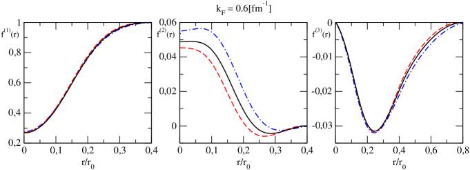
In Figure (2) we show the Jastrow, spin and tensor correlations at $k_{\text{F}}=0.6~{}\text{fm}^{-1}$ for the A8 potential. The dash-dotted lines are the normal phase correlations, whereas the solid lines give the correlations after solving the correlated gap equations. For the $S$–pairing case Jastrow and tensor correlations do not change from the normal to the BCS phases. Instead, the spin correlation shows some sensitivity to the environmental phase. It is reasonable to expect that for the ${}^{3}P_{2}$ ${}^{3}F_{2}$ pairing the tensor correlation also will depend on the phase.
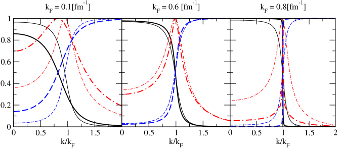
The $u^{2}$, $2uv$ and $v^{2}$ amplitudes, both for the pure and correlated BCS cases, are shown in Figure (3) at three Fermi momenta. At the lowest value, $k_{\text{F}}=0.1~{}\text{fm}^{-1}$, the uncorrelated and correlated amplitudes substantially differ among each other, the correlated ones showing a larger deviation from the step function, consistent with the larger gap value ($\Delta^{0}_{\text{F}}=0.07~{}\text{MeV}$ and $\Delta^{\textrm{CO}}_{\text{F}}=0.14~{}\text{MeV}$). At $k_{\text{F}}=0.6~{}\text{fm}^{-1}$ the amplitudes are very close in both approaches, yielding similar gaps ($\Delta^{0}_{\text{F}}=2.27~{}\text{MeV}$ and $\Delta^{\textrm{CO}}_{\text{F}}=2.25~{}\text{MeV}$). At the largest value, $k_{\text{F}}=0.8~{}\text{fm}^{-1}$, the correlated amplitudes are practically step functions. In fact this is almost the highest density for which we find solution to the correlated BCS equations.
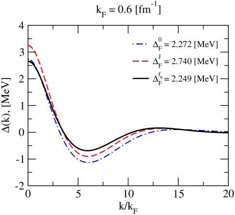
The gap function, $\Delta(k)$, at $k_{\text{F}}=0.6~{}\text{fm}^{-1}$ is given in Figure (4). In addition to the pure and correlated BCS functions, we show the one obtained by a simple Jastrow–correlated wave–function. At low $k$–values, $k/k_{\text{F}}<2.5$, the effects of the Jastrow and spin–dependent correlations compensate, providing a gap function close to the BCS result. At larger momenta they add and the correlated gap function departs from the uncorrelated one, up to $k/k_{\text{F}}\sim 15$, where all functions have essentially vanished.
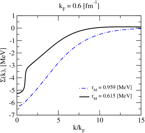
The self–energy, $\Sigma(k)$, is depicted in Figure (5) at $k_{\text{F}}=0.6~{}\text{fm}^{-1}$. The main difference between the BCS and correlated BCS cases lies in the sharp rising of the correlated $\Sigma(k)$ at $k\sim k_{\text{F}}$, which produces the much lower effective mass given in Table (1), $(m^{\star}/m)^{0}=0.96$ and $(m^{\star}/m)^{\textrm{CO}}=0.62$. The mass renormalization, caused by short-range correlations, enhanced the dispersive effect of the mean field, which leads to quenching of the energy gap, which is enhanced by the screening effect of the neutron pairing potential.

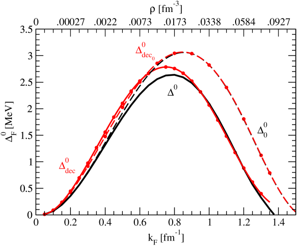
Figure (6) displays the energy gap at the Fermi surface, $\Delta_{\text{F}}^{(0)}$, as a function of the Fermi momentum for the A8 potential in the uncorrelated BCS case. The curves correspond to the full and to the decoupling approximation solutions of Ref. Kennedy (1968); Chen et al. (1986), with and without the self–energy insertions of eq. (81). The two gaps are very close for $\Sigma(k)=0$, whereas, after the introduction of the self–energy, the decoupling approximation appears to slightly overestimate the full solution.

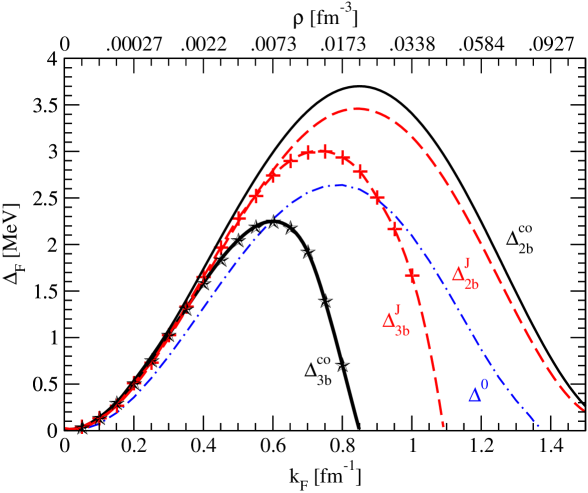
Figure (7) gives the gaps for different types of correlations (Jastrow and $f_{6}$) and at various levels of the cluster expansion for the same potential. The $\Delta^{0}$ gaps are the standard BCS results, those with the superscript ‘J’ are obtained within the Jastrow correlated theory and the ‘CO’ superscript denotes the corresponding correlations. The $2b$ and $3b$ subscripts in the correlated gaps refer to the pure two–body cluster case and to the one in which the density and the vertex corrections are computed at the first order of the power series expansion of Fig. (1). The inclusion of the Jastrow and $f_{6}$ correlations in the $2b$ case enhance the gap, because the short–range repulsion of the potential is renormalized by the short–range correlations. The $3b$ cases include medium modification effects via higher order cluster terms. Their effect is quite sizeable and reverse the behavior, both reducing the density region where we find a BCS solution and decreasing the maximum gap with respect to the standard case for the spin–dependent correlations. In fact, $\Delta^{0}(\text{max})\sim 2.6~{}\text{MeV}$ at $k_{\text{F}}\sim 0.9~{}\text{fm}^{-1}$, while $\Delta^{3b}_{f_{6}}(\text{max})\sim 2.2~{}\text{MeV}$ at $k_{\text{F}}\sim 0.6~{}\text{fm}^{-1}$. These results indicate that higher order many–body cluster terms may be relevant to estimate the gap.

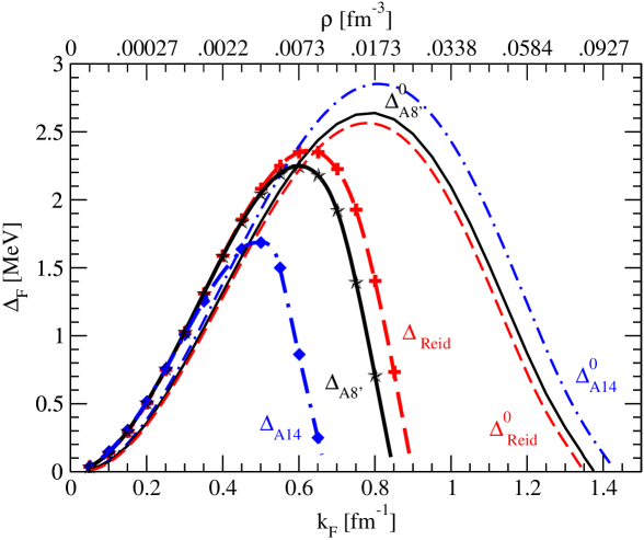
Finally, in Figure (8) we show the gaps for different potentials in the BCS and $f_{6}$–correlated theories. We have used, besides the Argonne $v_{8^{\prime}}$ model, also the Reid and Argonne $v_{14}$ (A14) potentials. These potentials differ mostly for the strength of the one–pion exchange induced components. In fact, A14 has much stronger spin and tensor potentials than Reid and A8. This difference shows up in the gaps, in both approaches. The BCS gap is larger in A14 than for the other potentials, and more drastically reduced in the correlated case, where $\Delta_{\text{A14}}(\text{max})\sim 1.7~{}\text{MeV}$ at $k_{\text{F}}\sim 0.5~{}\text{fm}^{-1}$.

Our results for the A14 potential are qualitatively similar to those of Ref. Lombardo and Schulze (2001) (see also Ref. Cao et al. (2006), where the more recent calculations was done), where the medium polarization was included via Landau theory. The authors found an analogous decrease of the BCS gap, with $\Delta_{\text{A14}}^{\textrm{Landau}}(\text{max})\sim 1.5-2~{}\text{MeV}$ at $k_{\text{F}}\sim 0.8~{}\text{fm}^{-1}$, but with a wider density region allowing for a superfluid solution.

V Conclusions and perspectives

The problem of an accurate determination of the BCS gap in a strongly interacting matter of nucleons is a longstanding one. Medium modification effects are expected to be important, but of difficult quantitative evaluation. We have used FHNC/BCS theory to take care of the short range correlations induced by the interaction in neutron matter at zero temperature. We have adopted the realistic Argonne $v_{8^{\prime}}$ two–nucleon potential and a correlation factor having central, spin and tensor dependent components. The density has been computed at the first order of the power series expansion, since this expansion provides at each order the correct density normalization in the normal phase. Consistently, the matrix elements of the hamiltonian in the correlated BCS state are evaluated at the two–body cluster level plus vertex corrections at the interacting pair. This treatment, in conjunction with the use of spin and tensor correlations lowers the maximum gap at $k_{\text{F}}$ by $\sim 20\%$ with respect to the uncorrelated BCS case. Moreover, $\Delta_{\text{F}}$ is shifted to a lower density. It is clear from our results the relevance of state dependent correlations for a reliable estimate of $\Delta_{\text{F}}$ in neutron matter, as well as the need for inserting medium modifications via higher order terms of the cluster expansion. Simple Jastrow, spin independent correlations always enhance $\Delta_{\text{F}}$, even if massive summations of cluster diagrams are performed. This effect is due to the screening of the short–range repulsive interaction provided by the Jastrow correlations. Similar conclusions are drawn when the short–range correlations are introduced by medium effects within the Brueckner G–matrix theory. State dependent correlations reverse this scenario and, after the inclusion of the vertex corrections, reduce $\Delta_{\text{F}}$. A qualitatively analogous result is found when state dependence is introduced by a CBF based perturbative expansion theory on top of Jastrow correlated states, but with spin dependent interactions.

In conclusion, we have stressed in this paper the importance of state dependent correlations and medium effects in superfluid neutron matter. Both of these tend to reduce the ${}^{1}S_{0}$ pairing gap, confirming previous studies.

The large effects found either by extending the study to the full FHNC/SOC calculations or after the introduction of the vertex corrections, strongly point to the need of a realistic estimate of many body effects. This can be done by using the calculated correlated BCS amplitudes as the guiding function of an AFDMC calculation. In the latter approach it is crucial to have a realistic guiding function in the path constraint. An extension of AFDMC to deal with the superfluid phases of neutron matter has been recently made and preliminary results, obtained for $14$ neutrons, are given in Ref. Fabrocini et al. (2005). A full description of both the AFDMC/BCS method and the corresponding results obtained for large systems will be given in a forthcoming paper Fantoni et al. (2007). An important issue is the role of the long range correlations. This can be most easily done in a Jastrow correlated BCS case. Work in this direction is in progress.

Acknowledgments

This work has been partially supported by the Italian MIUR through the PRIN: Fisica Teorica del Nucleo Atomico e dei Sistemi a Molti Corpi. K.E.S. acknowledges partial support by the US National Science Foundation via grant PHY-0456609. A.Yu.I. is grateful to INFN and to the Dipartimento di Fisica “E.Fermi” of the University of Pisa and acknowledges partial support from the PRIN 2006 Quantum noise in mesoscopic systems.

Refer to caption
Figure 2: (colored online) The central, spin and tensor correlation functions at the $k_{\text{F}}=0.6~{}\text{fm}^{-1}$ for the A8 potential. The dash-dotted, blue lines are the normal phase correlations. The dashed and solid, black lines are the BCS correlations without and with vertex corrections, correspondingly.
Refer to caption
Figure 3: (colored online) $v^{2}(k)$ (solid, black lines), $2v(k)u(k)$ (dash-dotted, red lines) and $u^{2}(k)$ (dashed, blue lines) amplitudes obtained from the A8 potential at three densities. The thin lines are the pure BCS results; the thick ones represent the correlated BCS amplitudes.
Refer to caption
Figure 4: (colored online) $\Delta(k)$, in MeV, obtained for the A8 model at $k_{\text{F}}=0.6~{}\text{fm}^{-1}$. The dash-dotted, blue line is the pure BCS solution; the dashed, red line represents the Jastrow correlates BCS case; the solid, black line is the fully correlated BCS solution.
Refer to caption
Figure 5: (colored online) The self-energy $\Sigma(k)$, in MeV, for the BCS (dash-dotted, blue line) and correlated BCS (solid, black line) cases for the A8 model at $k_{\text{F}}=0.6~{}\text{fm}^{-1}$.
Refer to caption
Figure 6: ${}^{1}S_{0}$ pairing gaps obtained from the A8 potential in the uncorrelated BCS case. The curves labeled $\Delta^{0}_{\text{dec}_{0}}$ and $\Delta^{0}_{\text{dec}}$ are calculated in the decoupling approximation, without and with self–energy insertions, respectively. The remaining curves refer to the full solution ($\Delta^{0}_{0}$ with $\Sigma(k)=0$ and $\Delta^{0}$ with $\Sigma(k)\neq 0$).
Refer to caption
Figure 7: A8 ${}^{1}S_{0}$ pairing gaps for different correlations and levels of the cluster expansions. See text.
Refer to caption
Figure 8: ${}^{1}S_{0}$ pairing gaps for different nucleon-nucleon potentials.
$k_{\text{F}}^{0}$ $[\text{fm}^{-1}]$ 0.1 0.2 0.3 0.4 0.5 0.6 0.7 0.8 0.9 1.0 1.1 1.2 1.3
$\rho_{0}$ $[\text{fm}^{-3}]$ .000034 .00027 .00091 .00216 .00422 .00730 .01158 .01729 .02462 .03377 .04495 .05836 .07420
$\lambda_{\text{F}}^{0}$ $[\text{MeV}]$ .1780 .6615 1.4771 2.6628 4.2509 6.2696 8.7478 11.721 15.239 19.379 24.254 30.030 36.907
$(m^{\star}/m)^{0}$ .9994 .9960 .9897 .9811 .9708 .9589 .9452 .9296 .9120 .8926 .8716 .8496 .8270
$\Delta_{\text{F}}^{0}$ $[\text{MeV}]$ .0719 .3568 .7986 1.3188 1.8359 2.2719 2.5576 2.6391 2.4850 2.0963 1.5209 .8713 .3247
$k_{\text{F}}^{\text{J}}$ $[\text{fm}^{-1}]$ .1001 .2002 .3006 .4011 .5020 .6030 .7041 .8049 .9048 1.0032
$\rho_{\text{J}}$ $[\text{fm}^{-3}]$ .000034 .00027 .00092 .00218 .00427 .00741 .01179 .01761 .02502 .03410
$\lambda_{\text{F}}^{\text{J}}$ $[\text{MeV}]$ .1289 .5100 1.1721 2.0775 3.2336 4.6656 6.3312 8.2222 10.3590 12.737
$(m^{\star}/m)^{\text{J}}$ .9774 .9480 .9072 .8609 .8065 .7370 .6516 .5426 .4035 .2591
$\Delta_{\text{F}}^{\text{J}}$ $[\text{MeV}]$ .1319 .5067 1.0236 1.6511 2.2785 2.7398 2.9884 2.9373 2.5069 1.6666
$k_{\text{F}}^{\text{CO}}$ $[\text{fm}^{-1}]$ .1001 .2002 .3006 .4011 .5017 .6022 .7020 .8004
$\rho_{\text{CO}}$ $[\text{fm}^{-3}]$ .000034 .00027 .00092 .00218 .00427 .00738 .01168 .01732
$\lambda_{\text{F}}^{\text{CO}}$ $[\text{MeV}]$ .1204 .4808 1.0709 1.8602 2.8082 3.8527 4.9220 5.9532
$(m^{\star}/m)^{\text{CO}}$ .9787 .9470 .9023 .8409 .7533 .6146 .3997 .2476
$\Delta_{\text{F}}^{\text{CO}}$ $[\text{MeV}]$ .1379 .5104 1.0291 1.5861 2.0471 2.2487 1.9257 0.7098
Table 1: Fermi momentum, $k_{\text{F}}$, density, $\rho$, chemical potential, $\lambda_{\text{F}}$, effective mas, $m^{\star}/m$, and gap value, $\Delta_{\text{F}}$, in different approximations (see text).

References

  • Fantoni (1981) S. Fantoni, Nucl. Phys. A363, 381 (1981).
  • Migdal (1960) A. B. Migdal, Sov. Phys. JETP 10, 176 (1960), [Zh. Eksp. Theor. Fiz., 37, 249 (1960)].
  • Tsuruta (1998) S. Tsuruta, Phys. Rept. 292, 1 (1998).
  • Heiselberg and Hjorth-Jensen (2000) H. Heiselberg and M. Hjorth-Jensen, Phys. Rept. 328, 237 (2000), eprint [nucl-th/9902033].
  • Sauls (1989) J. A. Sauls, in Cesme Lectures on “Timing Neutron Stars”, NATO-ASI, Series C, April 1988, edited by H. Ögelman, E. P. J. van den Heuvel, and J. van Paradis (Kluwer Academic Press, 1989), vol. 262, pp. 441–490.
  • Alpar and Pines (1993) M. A. Alpar and D. Pines, in Proc. The Los Alamos Workshop “Isolated Pulsars”, edited by K. A. Van Riper, R. Epstein, and C. Ho (Cambridge University Press, 1993).
  • Bohr et al. (1958) N. Bohr, B. R. Mottelson, and D. Pines, Phys. Rev. 110, 936 (1958).
  • Cooper et al. (1959) L. N. Cooper, R. L. Mills, and A. M. Sessler, Phys. Rev. 114, 1377 (1959).
  • Bardeen et al. (1957) J. Bardeen, L. N. Cooper, and J. R. Schrieffer, Phys. Rev. 108, 1175 (1957).
  • Feenberg (1969) E. Feenberg, in Theory of Quantum Fluids (Academic Press, 1969).
  • Baldo (1999) M. Baldo, in Nuclear Methods and the Nuclear Equation of State, edited by M. Baldo (World Scientific, 1999).
  • Vonderfecht et al. (1993) A. Vonderfecht, W. Dickhoff, and A. Polls, Nucl. Phys. A555, 1 (1993).
  • Wiringa et al. (2000) R. B. Wiringa, S. C. Pieper, J. Carlson, and V. R. Pandharipande, Phys. Rev. C62, 044310 (2000).
  • Wiringa et al. (1988) R. B. Wiringa, F. Ficks, and A. Fabrocini, Phys. Rev. C38, 1010 (1988).
  • Fabrocini et al. (2000) A. Fabrocini, F. Arias de Saavedra, and G. Co’, Phys. Rev. C61, 044302 (2000).
  • Chen et al. (1986) J. M. C. Chen, J. W. Clark, E. Krotscheck, and R. A. Smith, Nucl. Phys. A451, 509 (1986).
  • Chen et al. (1993) J. M. C. Chen, J. W. Clark, R. D. Davé, and V. V. Khodel, Nucl. Phys. A555, 59 (1993).
  • Reid (1968) R. V. J. Reid, Ann. of Phys. 50, 411 (1968).
  • Pandharipande and Wiringa (1979) V. R. Pandharipande and R. B. Wiringa, Rev. Mod. Phys. 51, 821 (1979).
  • Fantoni and Rosati (1975) S. Fantoni and S. Rosati, Nuovo Cim. A25, 593 (1975).
  • Alpar et al. (1990) M. A. Alpar, W. Brinkmann, Ü. Kizilogo, H. Ögelman, and D. Pines, Astron. Astrophys. 229, 133 (1990).
  • Fantoni and Pandharipande (1984) S. Fantoni and V. R. Pandharipande, Nucl. Phys. A427, 473 (1984).
  • Sarsa et al. (2003) A. Sarsa, S. Fantoni, K. E. Schmidt, and F. Pederiva, Phys. Rev. C68, 024308 (2003).
  • Carlson et al. (2003) J. Carlson, S.-Y. Chang, V. R. Pandharipande, and K. E. Schmidt, Phys. Rev. Lett. 91, 050401 (2003).
  • Fabrocini et al. (2005) A. Fabrocini, S. Fantoni, A. Y. Illarionov, and K. E. Schmidt, Phys. Rev. Lett. 95, 192501 (2005).
  • Lagaris and Pandharipande (1981) I. E. Lagaris and V. R. Pandharipande, Nucl. Phys. A359, 331 (1981).
  • Akmal et al. (1998) A. Akmal, V. R. Pandharipande, and D. G. Ravenhall, Phys. Rev. C58, 1804 (1998), eprint nucl-th/9804027.
  • Fantoni and Fabrocini (1998) A. Fantoni and A. Fabrocini, Lecture Notes in Phys. Vol. 510, 119 (1998).
  • Leggett (1975) A. J. Leggett, Rev. Mod. Phys. 47, 331 (1975), [Erratum: Rev. Mod. Phys. 48, 357 (1976).].
  • Khodel et al. (1996) V. A. Khodel, V. V. Khodel, and J. W. Clark, Nucl. Phys. A598, 390 (1996).
  • Kennedy (1968) R. C. Kennedy, Nucl. Phys. A118, 189 (1968).
  • Lombardo and Schulze (2001) U. Lombardo and H.-J. Schulze, in Physics of neutron Stars Interior, edited by D. Blaschke, N. K. Glendenning, and A. Sedrakian (Springer (Berlin), 2001), vol. 578, p. 30.
  • Cao et al. (2006) L. G. Cao, U. Lombardo, and P. Schuck, Phys. Rev. C74, 064301 (2006).
  • Fantoni et al. (2007) S. Fantoni, A. Y. Illarionov, and K. E. Schmidt, in preparation (2007).