How complex a complex network of equal nodes can be?

Abstract

Positive Lyapunov exponents measure the asymptotic exponential divergence of nearby trajectories of a dynamical system. Not only they quantify how chaotic a dynamical system is, but since their sum is an upper bound for the entropy by the Ruelle inequality, they also provide a convenient way to quantify the complexity of an active network. We present numerical evidences that for a large class of active networks, the sum of the positive Lyapunov exponents is bounded by the sum of the positive Lyapunov exponents of the corresponding synchronization manifold, the last quantity being in principle easier to compute than the latter. This fact is a consequence of the property that for an active network considered here, the amount of information produced is more affected by the interactions between the nodes than by the topology of the network. Using the inequality described above, we explain how to predict the behavior of a large active network only knowing the information provided by an active network consisting of two coupled nodes.

1 Introduction

The relation between topology and function in active networks, networks composed by nodes described by some intrinsic deterministic dynamics, is a fundamental question whose answer may help understand the collective behavior [1] of a variety of complex systems ranging from particle-like chemical waves [2], light propagation in dieletric structures [3], neural networks [4] and metabolic networks [5].

The work of Kuramoto [6] and the works of Pecora and collaborators [7, 8] laid the foundations of a theoretical framework for studying the relation between topology and function in active networks. In particular, the latter opened up a new way to study the onset of complete synchronization in active networks [9, 10, 11] composed of equal node dynamics.

At the present moment, it is important to understand from a theoretical perspective the relation between the structure of a network (topology) and the behavior of it (function) in active networks whose nodes are not only far away from complete synchronization (desynchronous) but also nodes that interact among themselves simultaneously by linear and nonlinear means.

In this work, we conjecture that an upper (or lower) bound for the sum of the Lyapunov exponents of an active network with some special properties [12] and an arbitrary size, formed by nodes possessing equal dynamics, can be analytically calculated by only using information coming from the behavior of two coupled nodes. We recall that by the Ruelle Formula [13], the sum of the positive Lyapunov exponents is an upper bound for the entropy. Hence, the sum of the positive Lyapunov exponents represent a convenient way to quantify the behavior of the network and therefore to measure how complex a network is.

To describe our conjecture, we first introduce some concepts and ideas, illustrated by Fig. 1. This figure represents the trajectory of two nodes $X$ and $Y$ of a large network. The networks considered here admit a synchronous solution [see Eq. (1)] and a desynchronous one. The position where this synchronous solution lies is pictorially represented by the dashed black line that represents a projection of the synchronization manifold of the network. The desynchronous solution is represented by the filled red regions localed off the diagonal. This solution represents a chaotic desynchronous trajectory.

If the synchronous solution is unstable, initial conditions close to the synchronization manifold leave its neighborhood, eventually arriving at a desynchronous (stable) solution, a chaotic attractor. If the synchronous solution is stable, it is to be expected that complete synchronization takes place, when all nodes have equal trajectories.

The Lyapunov exponents of the desynchronous solutions (a chaotic attractor) are calculated from Eq. (2), and the sum of the positive ones is denoted by $\Lambda$. The Lyapunov exponents of the synchronous solution are refered to as conditional Lyapunov exponents, and the sum of the positive ones is denoted by $\Lambda_{C}$. [16].

Roughly speaking, our conjecture states that if for two ($N=2$) coupled nodes with equal dynamics and coupling strengths, the quantity $\Lambda$ is greater (smaller) than $\Lambda_{C}$, then this inequality remains valid for $N>2$ coupled nodes (with the same dynamics) with coupling strengths obtained by properly rescaling.

Accordingly, given an interval for each coupling strength, the collection of all networks considered here can be classified in two classes : The class LOWER for which $\Lambda\geq\Lambda_{C}$ ($\Lambda_{C}$ is a lower bound for $\Lambda$) and the class UPPER for which $\Lambda\leq\Lambda_{C}$ ($\Lambda_{C}$ is an upper bound for $\Lambda$). While for the first class, a node forces another not to do what it is doing, inducing the nodes to stay out of synchrony, in the second class a node forces another to do what it is doing, inducing all the nodes to become synchronous.

Naturally, if the nodes in the network becomes completely synchronous, then the synchronous solution becomes stable and $\Lambda=\Lambda_{C}$.

It is often considered that the complexity of a network can be quantified by typical characteristics as the average degree, the network’s connecting topology, the minimal and maximal degree, the average or minimal path length connecting two nodes, and others. But these characteristics are a measure of the structure of the network and not of the behavior of it. In this work, at least for the class of networks considered here, we can state that these active networks behave in only two ways, regardless the many characteristics that quantify the network’s structure: the behaviors UPPER and LOWER. In other words, if nodes of an active network with equal nodes interact by a coupling function that induces an LOWER (or UPPER) character, this character will not be modified by the use of other connecting topologies.

To justify our conjecture, we use complex networks of linear and nonlinear maps coupled by linear terms, and neural networks of highly non-linear neurons (Hindmarsh-Rose (HR) neurons [17]) connected simultaneously by linear couplings (electrical synapses) and non-linear couplings (chemical synapses).

We finally discuss how our conjecture can be used to predict whether a network formed by nodes that when isolated are chaotic (periodic) will maintain such a chaotic behavior, then predicting how complex larger networks can be.

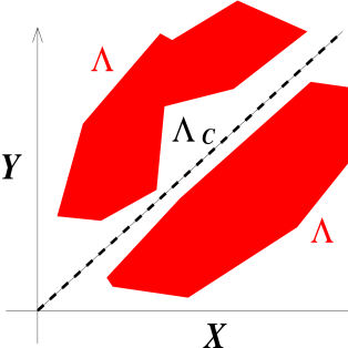
Figure 1: [Color online] Illustration of the two most relevant types of solutions we expect to find in the networks here considered. A synchronous solution whose trajectory is represented by the black dashed line, which lies on the synchronization manifold, and the desynchronous solution whose trajectory is represented by the red filled regions. The sum of the positive Lyapunov exponents of the synchronous solution is denoted by $\Lambda_{C}$ and the sum of the positive Lyapunov exponents of the desynchronous solution is denoted by $\Lambda$.

2 Active networks

Consider an active network formed by $N>0$ equal nodes $\mathbf{x_{i}}\in\mathbb{R}^{d}$ with $d>2$. The network is described by

$$\dot{\mathbf{x_{i}}}=\mathbf{F(x_{i})}+\sigma\sum_{j=1}^{N}\mathcal{G}_{ij}\mathbf{H(x_{j})}+g\sum_{j=1}^{N}\mathcal{C}_{ij}\mathbf{S(x_{i},x_{j})},$$ (1)

where $g\in\mathbb{R}$ and $\sigma>0$, $\mathcal{G}=\{\mathcal{G}_{ij}\}$ is a Laplacian matrix ($\sum_{j}\mathcal{G}_{ij}=0$) describing the way nodes are linearly coupled, $\mathcal{C}=\{\mathcal{C}_{ij}\}$ is the the adjacent matrix representing the way the nodes are connected by linear and non-linear function, and $\mathbf{H}:\mathbb{R}^{d}\to\mathbb{R}^{d}$ and $\mathbf{S}:\mathbb{R}^{d}\times\mathbb{R}^{d}\to\mathbb{R}^{d}$ are arbitrary differentiable transformations. We also assume that $\mathcal{G}$ and $\mathcal{C}$ commute.

A solution of (1) is called synchronous if $\mathbf{x_{1}}(t)=\cdots=\mathbf{x_{N}}(t)$. To guarantee the existence of such solutions, we assume that every node of the network receives the same number $k$ of incoming connections. In other words, we require that $\sum_{j}\mathcal{C}_{ij}=k$ for any $i$. It is easy to see that this condition not only guarantees the existence of synchronous solution, but also implies that the $d$-dimensional linear subspace $\mathcal{S}=\{\mathbf{x_{1}=x_{2}=\ldots=x_{N}}\}$ is invariant. The set $\mathcal{S}$ is called synchronization manifold. Note that a synchronous solution $\mathbf{x}_{i}(t)=\mathbf{x}(t)$ for $i=1,\ldots,N$ satisfies the following ordinary differential equation

$$\dot{\mathbf{x}}=F(\mathbf{x})+gk\mathbf{S(x,x)}.$$ (2)

The way small perturbations $\mathbf{\delta x}_{1},\mathbf{\delta x}_{2},\ldots,\mathbf{\delta x}_{N}$ propagate in the network is described by the variational equations [7] associated to (1)

$$\dot{\mathbf{\delta x}}_{i} = DF(\mathbf{x}_{i})\mathbf{\delta x}_{i}+\sigma\sum_{j=1}^{N}\mathcal{G}_{ij}D{\mathbf{H}}(\mathbf{x}_{j})\mathbf{\delta x}_{j}+$$

$$g\sum_{j=1}^{N}\mathcal{C}_{ij}D_{1}\mathbf{S}(\mathbf{x}_{i},\mathbf{x}_{j})\mathbf{\delta x}_{i}+g\sum_{j\neq i}\mathcal{C}_{ij}D_{2}\mathbf{S}(\mathbf{x}_{i},\mathbf{x}_{j})\mathbf{\delta x}_{j},$$

where $D_{1}S(x,y)$ and $D_{2}S(x,y)$ denote the differential of $S(x,y)$ with respect to $x$ and $y$, respectively. From (2), we can calculate the Lyapunov exponents of every solution of (1). The network is assumed to be ergodic, and so the Lyapunov exponents $\lambda_{1}\leq\lambda_{2}\leq\cdots\leq\lambda_{m}$ for $m=1,\ldots,Nd$ are constant almost everywhere, and can be obtained by typical initial conditions. The $Nd$ Lyapunov exponents of the synchronous solutions are called conditional Lyapunov exponents. We also assume that the dynamics restricted to the synchronization manifold $\mathcal{S}$ is ergodic. Hence, also the conditional Lyapunov exponents along synchronous solutions are constant almost everywhere on $\mathcal{S}$. The ergodic invariant measure of (1) and that of the dynamics restricted to $\mathcal{S}$ (not necessarely the same) are assumed to be unique (singular) and different than a point (non-atomic).

3 Conjecture

Here, we describe our proposed conjecture in a more friendly way. For a more rigorous presentation of it, one should read the Appendix 9.1.

Let $\mathbf{H,S,\mathcal{G},\mathcal{C}},\sigma,g,N$ as in (1) to be the parameters which define the active network. $\mathbf{H}$ represents the function under which the nodes connect among themselves in a linear fashion, $\mathbf{S}$ the function under which the nodes connect among themselves in a non-linear fashion, $\mathbf{\mathcal{G}}$ a Laplacian connecting matrix, $\mathbf{\mathcal{C}}$ an adjacent connecting matrix, $\mathbf{\sigma}$ the strength of the linear coupling and $g$ the strength of the non-linear coupling. Finally, $N$ is the number of nodes.

We say that a network is of the class UPPER if $\Lambda\geq\Lambda_{C}$ and of the class LOWER if $\Lambda\leq\Lambda_{C}$.

We consider that the UPPER and LOWER property holds for a properly rescaled coupling strength intervals $\sigma(N,\mathcal{G},\mathcal{C})$ $\in$ $[\sigma_{m}(N,\mathcal{G},\mathcal{C}),\sigma^{*}(N,\mathcal{G},\mathcal{C})]$ and $g(N,\mathcal{G},\mathcal{C})$ $\in$      $[g_{m}(N,\mathcal{G},\mathcal{C}),g^{*}(N,\mathcal{G},\mathcal{C})]$.

Conjecture: The LOWER or UPPER character of a network described by Eq. (1) is independent of the number of nodes for a properly rescaled coupling strength interval.

In simple words, this conjecture states that as long as one preserves the coupling functions $\mathbf{H,S}$ under which nodes connect among themselves, there will be coupling strengths $\sigma,g$ for which the LOWER or UPPER character of an active network will be preserved, regardless of the number of nodes $N$.

4 Defining the coupling strength intervals

For simplicity in the notation, we ommit in the representation of the constants $\sigma_{m},\sigma^{*}$ and $g_{m},g^{*}$ the reference to their dependence on $\mathbf{\mathcal{G},\mathcal{C}}$.

Our conjecture only states that whenever there is a network with $N_{1}$ nodes with a structure defined by $\mathbf{H,S,\mathcal{G},\mathcal{C}}$ and this network has an UPPER (or lower) character for the coupling strength intervals $[\sigma_{m}(N_{1}),\sigma^{*}(N_{1})]$ and $[g_{m}(N_{1}),g^{*}(N_{1})]$ then if a network with $N_{2}$ nodes is constructed preserving the coupling functions $\mathbf{H,S}$ then there exists coupling strength intervals $[\sigma_{m}(N_{1}),\sigma^{*}(N_{1})]$ and $[g_{m}(N_{1}),g^{*}(N_{1})]$ for which the network behaves with the same UPPER (or lower) character.

To make this conjecture more practical, we make in the following some assumptions.

The value of the constants $\sigma_{m}(N),\sigma^{*}(N)$ and $g_{m}(N),g^{*}(N)$ are such that either      $|\sigma_{m}(N)/g_{m}(N)|$ $>>$ 1 or $|\sigma_{m}(N)/g_{m}(N)|$ $<<$ 1 and $|\sigma^{*}(N)/g^{*}(N)|$ $>>$ 1 or $|\sigma^{*}(N)/g^{*}(N)|$ $<<$ 1. The reason is because for such conditions, the values for these constants for a network with $N>2$ nodes can be calculated from the values of these constants from the reference network, in here assumed to have $N=2$ nodes.

The network with $N_{1}$ nodes is regarded to be the reference network and we consider that $N_{2}>N_{1}$. For simplicity, we further consider that $N_{1}=2$. In addition, to make our analyses simpler, we consider in our numerical simulations a constant $g_{m}(N)=g^{*}(N)$, and we choose either $|\sigma_{m}(N)/g_{m}(N)|>>$1 or $|\sigma_{m}(N)/g_{m}(N)|<<$1.

Then, we choose the constant $\sigma^{*}(N)$ such that its value is a little bigger than the smallest coupling values for which complete synchronization is reached and when $\Lambda=\Lambda_{C}$. However, other intervals could be considered. The reason again is that $\sigma^{*}(N)$ can be analytical calculated from $\sigma^{*}(N=2)$, the linear coupling strength, for which complete synchronization is found in two mutually coupled systems.

The constants that define the coupling strength interval for a network with $N$ nodes can be calculated from the constants that define the coupling strength interval for a network with $N=2$ nodes using

$$\sigma(N)=\frac{2\sigma(N=2)}{|\gamma_{2}(N)|}$$ (4)

$$g(N)=\frac{g(N=2)}{k}$$ (5)

where $\gamma_{2}$ is the second largest eigenvalue of $\mathcal{G}$, and $k$ is the number of incoming connections of each node of the network.

As an example of how we use Eq. (4), we do the following. Having defined that two mutually linearly coupled systems (so, $g$=0) have a LOWER character for the linear coupling strength interval $[\sigma_{m}(N=2),\sigma^{*}(N=2)]$,then we construct a network using the same linear coupling function composed of $N$ nodes, but considering now the linear coupling strength interval $[\sigma_{m}(N),\sigma^{*}(N)]$ calculated using Eq. (4). According to our conjecture, such a network will have a lower character.

For a more detailed analysis of how we derive Eqs. (4) and (5), one should read Appendix 9.2.

5 Networks of coupled maps

Here, we consider only linear couplings. Then $g=g_{m}$=0, and therefore, $\sigma_{m}=0$.

For general networks (discrete or continuous descriptions) whose nodes are completely synchronous, one always have that $\Lambda=\Lambda_{C}$, a non generic case for which our conjecture can be proved.

For networks of coupled maps, there is another trivial example when $\Lambda=\Lambda_{C}$. That happens for networks whose Jacobian is constant as networks formed by linear maps of the type $x^{(i)}_{n+1}=\alpha x^{(i)}_{n}+2\sigma\sum_{j=1}^{N}\mathcal{G}_{ij}x^{(j)}_{n}$ (mod 1) and when there exists complete synchronization, and the attractor lays on the synchronization manifold. These results concern arbitrary connecting Laplacian matrices $\mathcal{G}_{ij}$, for example, they would apply for map lattice with a coupling whose strength decreases with the distance as a power-law [19].

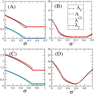
Figure 2: Results for the network in Eq. (6), for $\rho$=0.5. For (A) and (C), N=2, and for (B) and (D), $N$=16. An inhibitory (UPPER) network is shown in (A) and (B), for $s$=-1, and an excitable (LOWER) network is shown in (C) and (D), for $s$=1. The horizontal axis in (B) and (D) were rescaled by $\sigma^{\prime}$=$\sigma*|\gamma_{2}(N=16)|/2$, so that one can compare Figs. (B) and (D) with (A) and (C).$|\gamma_{2}(N=16)|$=4.1542.

Now, imagine the following network

$$x_{n+1}^{(i)}=2x_{n}^{(i)}+s\rho{x_{n}^{(i)}}^{2}+2\sigma\sum_{j=1}^{N}\mathcal{G}_{ij}x^{(j)}_{n}\text{ (mod 1)}$$ (6)

with $\rho\geq 0$ and $s=\pm 1$. The synchronization manifold is defined by $x_{n}^{(1)}=x_{n}^{(2)}=\ldots=x_{n}^{(N)}$, and in an all-to-all connecting topology, the Lyapunov exponent of the synchronization manifold can be calculated by $\lambda^{(1)}=\ln{(2)}+1/t\sum_{n}\ln{|1+s\rho x_{n}|}$, with $n=(1,\ldots,t)$, and the others $N-1$ equal exponents associated to the transversal directions by $\lambda^{(i)}=\ln{(2)}+1/t\sum_{n}\ln{|1+s\rho x_{n}-2\sigma|}$, for $i\geq 2$. In Fig. 2, we show the values of $\Lambda$ and $\Lambda_{C}$ as we vary $\sigma$, for $\rho=0.5$. In (A) and (C), we consider $N$=2 (all-to-all topology), and in (B) and (D) we consider a random networks formed by $N$=16 nodes. The coupling strength interval used for two coupled nodes was rescaled to the proper coupling strength interval for the larger random network, using in the denominator of Eq. (4) the value of $|\gamma_{2}|=4.1542$, relative to the second largest eigenvalue (in absolute value) of the random network. One can check that if two coupled nodes have an UPPER [LOWER] character for a given coupling interval as can be seen in Fig. 2(A) [in Fig. 2(C)], larger networks will behave in the same UPPER [LOWER] character as can be seen in Fig. 2(B) [in Fig. 2(D)].

The conjecture describes a relationship between the conditional exponents and the Lyapunov exponents. To see that, notice that, typically for the UPPER networks of linearly connected maps, we have $\lambda_{1}\approx\lambda^{(1)}$, a consequence of the fact that the largest Lyapunov exponent can be calculated using the same directions as the ones along the synchronization manifold. Thus, using our conjecture, if the network is of the UPPER type, $\lambda_{1}+\lambda_{2}\leq\lambda^{(1)}+\lambda^{(2)}$, which provides $\lambda_{2}\leq\lambda^{(2)}$. Otherwise, if the network is of the LOWER type, $\lambda_{2}\geq\lambda^{(2)}$. That can be checked in Figs. 2(A)-(C). Since the approaching of the transversal conditional exponents to negative values are associated with the stabilization of a certain oscillation mode, close to a coupling strength for which a transversal conditional exponent approaches zero, there will also be a Lyapunov exponent which approaches zero, meaning that some oscillation in the attractor becomes stable.

6 Networks of Hindmarsh-Rose neurons

Let us illustrate our conjecture in networks composed of $N$ coupled Hindmarsh-Rose neurons [17] electrically and chemically coupled [20]:

$$\dot{x}_{i} = y_{i}+3x_{i}^{2}-x_{i}^{3}-z_{i}+I_{i}+g\sum_{j=1}^{N}\mathcal{C}_{ij}S(x_{i},x_{j})$$ (7)

$$+\sigma\sum_{j=1}^{N}\mathcal{G}_{ij}x_{j}$$

$$\dot{y}_{i} = 1-5x_{i}^{2}-y_{i};\>\>\>\dot{z}_{i}=-rz_{i}+4r(x_{i}+1.6),$$

The parameter $r$ modulates the slow dynamics and is set equal to 0.005, such that each neuron is chaotic. The synaptic chemical coupling is modeled by $S(x_{i},x_{j})=(x_{i}-V_{syn})\Gamma(x_{j})$ where $\Gamma(x_{j})=\displaystyle\frac{1}{1+e^{-\theta(x_{j}-\Theta_{syn})}}$ with $\Theta_{syn}=-0.25$, $\theta=10$ and $V_{syn}=2.0$. $\sigma{\bf\mathcal{G}}_{ji}$ is the strength of the electrical coupling between the neurons, and $I_{i}=3.25$. In order to simulate the neuron network and to calculate the Lyapunov exponents through Eq. (11), we use for the node $i$ the initial conditions $x_{i}$=-1.3078+$\omega_{i}$, $y_{i}$=-7.3218+$\omega_{i}$, and $z_{i}$=3.3530+$\omega_{i}$, where $\omega_{i}$ is an uniform random number within [0,0.02]. To calculate the conditional exponents $\lambda^{(i)}$, we use in Eq. (12) the initial conditions, $x$=-1.3078, $y$=-7.3218, and $z$=3.3530, but any other set of typical equal initial conditions can be used [21].

We study three types of neural networks. (i) $g<0$ [Figs. 3(A-C)]. The coupling (synapses) is said to be of the excitatory type, since $x_{i}-V_{syn}<0$ and the nodes $j$ contribute positively in the equations for the first derivative of $x_{i}$. In other words, the postsynaptic neuron ($x_{i}$) is forced to opposite the presynaptic ones ($x_{j}$); (ii) $g=0$ [Figs. 3(D-F)]. The network has nodes coupled to other nodes only electrically. From the biological point of view, neurons only make electrical connections with their nearest neighbors. Here, we also consider long-range correlations. Since $\sigma\geq 0$, this coupling contributes negatively to the first derivative of $x_{i}$, which results in an inhibitory effect to the oscillatory motion of the neuron $x_{i}$. (iii) $g>0$ [Figs. 3(G-I)]. The coupling (synapses) is said to be of the inhibitory type, since the nodes $j$ contribute negatively in the equations for the first derivative of $x_{i}$. For such a case, the postsynaptic neuron ($x_{i}$) is forced to synchronize its rithmus to the rithmus of the presynaptic ones ($x_{j}$).

In Fig. 3, we show the values of $\Lambda$ and $\Lambda_{C}$ for the three types of neural networks being considered, case (i) in Figs. 3(A-C), case (ii) in Figs. 3(D-F), and case (iii) in Figs. 3(G-I). Networks whose results are represented in Figs. 3(A-C) and (G-I) are constructed by neurons connected simultaneously electrically ($\sigma>0$) and chemically ($g>0$) in the all-to-all topology, while networks whose results are represented in Figs. 3(D-F) are constructed by neurons connected only electrically ($\sigma>0$ and $g$=0) in the all-to-all topology.

In (A) [case (i)], for $N$=2 and $g=-0.01$, $\Lambda\leq\Lambda_{C}$, for $\sigma=[0.1,0.7]$. So, $\sigma_{m}(N=2)$=0.1 which leads to $\sigma_{m}(N=2)/g_{m}(N=2)|>>1$, as we wish. From our conjecture, for larger networks as the ones shown in Figs. 3(B) [$N=4$] and 3(C) [$N$=8], we must have $\Lambda\leq\Lambda_{C}$, for the rescaled coupling interval. From Eqs. (4) and (5), we have for the network with $N=4$ [Fig. 3(B)], the rescaled coupling strength interval should be $\sigma=[0.1/2,0.7/2]$ and $g=-0.01/3$, and for the network with $N=8$ [Fig. 3(C)], the rescaled coupling strength interval should be $\sigma=[0.1/4,0.7/4]$ and $g=-0.01/7$. In fact, as one sees in Figs. 3(B-C), we indeed see that these networks have the same UPPER character as the network with $N$=2, for the considered coupling strength intervals.

In (D) [case (ii)], for $N$=2 and $g=0$, $\Lambda\leq\Lambda_{C}$ for $\sigma=[0,0.6]$. So, $g_{m}(N=2)=0$ and consequently $\sigma_{m}(N=2)=0$. From our conjecture, for larger networks as the ones shown in Figs. 3(E) [$N=4$] and 3(F) [$N$=8], we must have $\Lambda\leq\Lambda_{C}$ for the rescaled coupling interval. From Eqs. (4) and (5), we have for $N=4$ [Fig. 3(E)], the rescaled coupling interval should be $\sigma=[0,0.6/2]$ and for $N=8$ [Fig. 3(F)], the rescaled coupling interval should be $\sigma=[0,0.6/4]$. In fact, as one sees in Figs. 3(E-F), we indeed have that these networks have the same UPPER character of the network with $N$=2.

Finally, In (G) [case (iii)], for $N$=2 and $g$=10, $\Lambda\geq\Lambda_{C}$ for $\sigma=[0.01,1]$. So, $|g_{m}(N=2)/\sigma_{m}(N=2)|>>1$ as we wish. From our conjecture, for larger networks, as the ones shown in Figs. 3(H) [$N=4$] and 3(I) [$N$=8], we must have $\Lambda\geq\Lambda_{C}$ for the rescaled coupling interval. From Eqs. (4) and (5), and $N=4$ [Fig. 3(H)], the rescaled coupling interval should be $\sigma=[0.01/2,1/2]$ and $g$=10/3, and for $N=8$ [Fig. 3(I)], the rescaled coupling interval should be $\sigma=[0.01/4,1/4]$ and $g$=10/7. In fact, as one see in Figs. 3(G-I), we indeed have that these networks have the same LOWER character of the network with $N$=2.

An inhibitory chemical coupling inhibits the nodes of the network, which means that such a coupling forders an increase in the level of synchronization. On the other hand, an excitatory chemical coupling excites the nodes, which means that such a coupling forders an increase in the level of desynchrony.

It is intuitive to imagine that an excitatory network (as defined exclusively in terms of the chemical coupling) would have a LOWER characteristic and an inhibitory network (as defined exclusively in terms of the chemical coupling) would have an UPPER characteristic. That is why excitation would mean an increase of desorganization (more entropy) and inhibition an increase of synchronization (less entropy). However, we have previously shown in Figs. 3(A-C) that an excitatory network (as usually defined in terms of the chemical coupling) has the UPPER characteristic and in Figs. 3(G-I) that an inhibitory network (as usually defined in terms of the chemical coupling) has the LOWER characteristic. This aparent contradiction is simple to be explained.

In the excitatory networks [Figs. 3(A-C)], the absolute strength of the non-linear (chemical) coupling (0.01) is smaller than the strength of the linear (electrical) coupling. As a consequence, the linear coupling prevails on the non-linear coupling. In the inhibitory networks [Figs. 3(A-C)], the strength of the non-linear (chemical) coupling (10) is much larger than the strength of the linear coupling. However, such a large strength effectively forders an excitatory behavior in the network. Notice that while in Fig. 3(A) complete synchronization appears for $\sigma\approx 0.5$, in Fig. 3(G) complete synchronization appears for $\sigma\approx 0.95$, and therefore, complete synchronization in the inhibitory network appears only for a larger linear coupling than the one for which complete synchronization appears in the excitatory networks.

It is not the scope of this work to determine for which conditions an inhibitory (or excitatory) non-linear (chemical) couplings in networks of neurons simultaneously connected by linear and non-linear means determines the UPPER or LOWER character of a network. For that one should check Ref. [18]. Had we consider that the neurons were connected exclusively by non-linear (chemical) means ($\sigma=0$), then it is to be expected that inhibitory networks would present an UPPER character and excitatory networks would present a LOWER character.

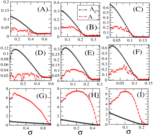
Figure 3: The values of $\Lambda$ and $\Lambda_{C}$ for neural networks described by Eq. (7) of nodes connected in an all-to-all topology. In (A),(D), and (G), $N$=2. In (B),(E), and (H), $N=4$. In (C), (F), (I), $N$=8. Results for networks with an UPPER character are shown in (A-F), and for networks with an LOWER character are shown in (G-I).

7 Application of our conjecture to predict the chaotic behavior of large networks

In the following, we discuss how our conjecture can be used to make general statements about active networks. Consider the UPPER networks formed by neurons connected only electrically ($g$=0). For such cases, $\Lambda_{C}(N)$ is an upper bound for the Kolmogorov-Sinai (KS) entropy $H_{KS}$ (see [13]) and also an upper bound for $\Lambda$. Since networks formed by nodes connected in an all-to-all topology produce Laplacian matrices whose eigenvalues are $\gamma_{1}=0$, and $\gamma_{i}$=$-N$, for $i=2,\ldots,N$, it is clear from Eq. (4) that $\max{[\Lambda_{C}(N)]}$ for the considered coupling strengths of a network with the all-to-all topology, is larger or equal to $\max{[\Lambda_{C}(N)]}$ for any other topology. Defining the network capacity, $c(N)$, to be equal to $\max{[\Lambda_{C}(N)]}$, calculated for the all-to-all topology (and the considered coupling intervals), since $\Lambda_{C}(N)\geq\Lambda(N)$ (as well as $\Lambda_{C}(L)\geq H_{KS}(N)$ [22]) for UPPER networks, we conclude that for these networks not only

$$c(N)\geq\max{[\Lambda(N)]}$$ (8)

but also

$$c(N)\geq\max{[H_{KS}(N)]}$$ (9)

where the $\max$ of $\Lambda(N)$ in taken considering ”any” possible topologies (described in Fig. 4) and the considered coupling intervals.

Figure 4: Representation of a few network topologies with 8 neurons, considered in this work. The filled balls represent neurons and the lines indicate an electric bidirectional coupling. In (A) the neurons are only coupled with its nearest neighbors, forming a ring. From (B) to (D) it is added to the network long-range bidirectional connections, The average number of connections that each neuron receives (network degree), $\omega$, is $\omega$=2, in (A), $\omega$=3, in (B), $\omega$=5, in (C), and $\omega$=7, in (D). In a network with $N$ neurons, long-range connections are introduced in the initial ring by connecting each neuron to its N/2-th (B) neighbors, then to its ($N/2$-1)-th neighbors (C), then to its ($N/2-l$)-th neighbors, till each neuron is connected to its second neighbors, when the network has the all-to-all coupling topology.

The value of $c(N)$ for neural networks electrically connected can be approximately calculated by $\max{(\lambda^{(1)})}+(N-1)\max{(\lambda^{2})}$ (notice that since ${\lambda^{(1)}}$ does not depend on $\sigma$, then, $\max{(\lambda^{(1)})}$ happens for the same coupling strength for which $\max{(\lambda^{(2)})}$ is found), which leads to $c(N)\cong 0.01362+0.1013(N-1)$ bits/(time unit). By doing simulations considering networks as the ones represented in Fig. 4, (with $10\leq N\leq 40$), we obtain that $\max{[\Lambda(N)]}\cong 0.0830+0.0230(N-1)$bits/(time unit), which agrees with Eq. (8).

For a network with the all-to-all topology [as in Fig. 4(D)], for $N\geq 10$, we obtain $\max{[\Lambda(N)]}\cong 0.158447+0.031537(N-1)$, which agrees with Eq. (8), because $c(N)\geq\max{[\Lambda(N)]}$ (where the maximum is taken considering the all-to-all topology). Finally, if we construct a network with nodes connecting to their nearest neighbors forming a closed ring [as in Fig. 4(A)], we find $\max{[\Lambda(N)]}\cong 0.197125+0.034865(N-1)$bits/(time unit). Equation (8) is once again verified.

Thus, $c(N)$ for electrically connected networks does not depend on the network topology. That is not the case for chemically connected neural networks, for which $c(N)$ might be achieved for different topologies, since the curve for $\lambda^{(1)}$ and $\lambda^{(i)}$ achieve their maximal values for different values of the coupling strength.

Further, consider two coupled LOWER-type systems and $\Lambda$ is null (positive) for some coupling strength, meaning a periodic behavior (meaning chaos). It might be that, for a proper rescaled coupling strength, as more nodes are added to the network, $\Lambda$ becomes positive, meaning chaos (for sure there will be chaos). We can also use our conjecture to predict the behavior of a network constructed with nodes that are either chaotic or periodic, by only having information about two coupled nodes. Considering only linear couplings [$g$=0, in Eq. (1)]. For $\sigma\leq\epsilon$, the two coupled nodes have a periodic dynamics, and thus, $\Lambda=0$, but $\Lambda_{C}>0$ (UPPER character). That implies that as we add more nodes in the network, it might be that after the proper rescaling of the coupling strength the network becomes chaotic.

8 Conclusions

In conclusion, we have presented arguments to suggest that for a class of dynamical systems, the sum of all the positive Lyapunov exponents of an active network is bounded by the sum of all the positive Lyapunov exponents of the synchronization manifold. In practical terms, the entropy production of the synchronization manifold and its transversal directions ($\Lambda_{C}$) of a system of two coupled equal dynamical systems determines the upper (LOWER character) or lower (UPPER character) bound for the sum of the positive Lyapunov exponents of a large network. This fact enables one to predict the behavior of a large network by using information provided by only two coupled nodes.

Our results indicate that the behavior (synchronization and information) of an active network with nodes possessing equal dynamics and especial properties [21] does not strongly depend on the coupling topology (${\mathcal{G}}$ and ${\mathcal{C}}$) and the size of the network ($N$) but rather on the nature of the coupling functions ($S$ and $H$).

At first glance, this result seems to be in direct conflict with what one would expect to find in realistic neural networks, as the mammalian brain, whose topology is possibly responsible for intelligence. But one should have in mind that the here considered networks are constructed with nodes that possess equal dynamics being connected using always the same coupling function. In realistic brain networks, the coupling functions largely differ along different brain areas as well as the coupling strength depends on time. Therefore, in order for the topology to play an important role in the behavior of a network one needs to consider networks with non-equal nodes and/or that possess coupling functions that change in space and time.

Naturally, the large class of networks for which our conjecture applies are far from being realistic. However, we believe our conjecture can contribute to the understanding of much more complex networks. For example, for the UPPER networks, a large series of numerical results show that more realistic networks constructed with non-equal nodes (or networks of equal nodes but with random coupling strengths [23]) have a KS entropy smaller than the networks with equal nodes. Therefore, even though networks with equal nodes might not be realistic, their entropy production is an upper bound for the entropy production of more realistic networks.

Excitability and inhibition is a concept usually used to classify the way non-linear (chemical) synapses between two neurons are done. When an inhibitory neuron spikes (the pre-synaptical neuron) a neuron connected to it (the post-synaptical neuron) is prevented to spike. When an excitatory neuron spikes it induces the post-synaptical neuron to spike. Intuitively, one should expect that an inhibitory (excitatory) coupling forders (prevents) synchronization, but we have shown two cases for which an excitatory network had an UPPER character and an inhibitory network had a LOWER character. The reason is that only the non-linear couplings (chemical synapses) are not sufficienty to define the LOWER and UPPER character of the network. One should consider the combined effect of the linear (electrical) and of the non-linear couplings (chemical). For more details about that, see Ref. [18]

For UPPER networks, the entropy of the attractors cannot be larger than the entropy of the synchronous set, which therefore imposes a clear limit in the complex character of these networks. On the hand, for LOWER networks, our conjecture states that such a limit is unknown.

This conjecture might be a consequence of the fact that the attractors and behaviors that appear in two coupled nodes for a given coupling strength are similar to the ones that appear for larger networks, to parameters rescaled according to Eqs. (4) and (5). In fact, as one can see in the work [24], that is indeed the case for the coupling strengths for which burst phase synchronization (BPS) or phase synchronization (PS) appear in networks of electrically coupled HR-neurons.

9 Appendix

9.1 The conjecture

Let $\mathbf{H,S,\mathcal{G},\mathcal{C}},\sigma,g,N$ as in (1) to be the parameters which defines the active network. $\mathbf{H}$ represents the function under which the nodes connects among themselves in a linear fashion, $\mathbf{S}$ the function under which the nodes connects among themselves in a non-linear fashion, $\mathbf{\mathcal{G}}$ a Laplacian connecting matrix, $\mathbf{\mathcal{C}}$ an adjacent connecting matrix, $\mathbf{\sigma}$ the strength of the linear coupling and $\mathbf{g}$ the strength of the non-linear coupling. Finally, $N$ is the number of nodes.

Denote by $\Lambda(\mathbf{H,S,\mathcal{G},\mathcal{C}},\sigma,g,N)$ and $\Lambda_{C}(\mathbf{H,S,\mathcal{G},\mathcal{C}},\sigma,g,N)$ the sum of the posititve Lyapunov exponents and the sum of the positive conditional Lyapunov exponents of the network whose structure is specified by $(\mathbf{H,S,\mathcal{G},\mathcal{C}})$, respectively. We say that the couple $(\mathbf{H,S})$ makes the network to be of the LOWER class if for every $(\mathbf{\mathcal{G},\mathcal{C}})$ there exist four positive constants $\sigma_{m}$, $g_{m}$, $\sigma^{*}$ and $g^{*}$ such that

$$\Lambda_{C}(\mathbf{H,S,\mathcal{G},\mathcal{C}},\sigma,g)\geq\Lambda(\mathbf{H,S,\mathcal{G},\mathcal{C}},\sigma,g)$$ (10)

for all $\sigma_{m}\leq\sigma\leq\sigma^{*}$ and all $g_{m}\leq g\leq g^{*}$. An UPPER class active network is defined similarly by reversing the direction of inequality (10).

Conjecture: Given a network with a LOWER (UPPER) character [as defined in (10)] specified by $(\mathbf{H,S,\mathcal{G},\mathcal{C}})$, and $(\mathbf{\mathcal{G},\mathcal{C}})$ with $N_{1}$ nodes, there exist coupling strength intervals $\tilde{\sigma_{m}}\leq\sigma\leq\tilde{\sigma^{*}}$ and $\tilde{g_{m}}\leq g\leq\tilde{g^{*}}$ for which a network specified by $(\mathbf{H,S,\mathcal{\tilde{G}},\mathcal{\tilde{C}}})$ and $(\mathcal{\tilde{G}},\mathcal{\tilde{C}})$ with $N_{2}$ nodes has also a LOWER (UPPER) character.

9.2 Derivation of the coupling strength constants

The variational equation (2) for the synchronous solution can be written as follows

$$\delta\mathbf{\dot{X}} = \{\mathbf{I}\otimes D\mathbf{F(\mathbf{x})}+\sigma{\mathcal{G}}\otimes D\mathbf{H(\mathbf{x})}+g{\mathcal{C}}\otimes D_{1}\mathbf{S(\mathbf{x},\mathbf{x})}$$ (11)

$$+ gk\mathcal{C}\otimes D_{2}\mathbf{S(\mathbf{x},\mathbf{x})}\}\delta\mathbf{X},$$

where $\mathbf{\delta X}$ is the column vector of $\mathbb{R}^{Nd}$ with components $\mathbf{\delta x}_{1},\mathbf{\delta x}_{2},\ldots,\mathbf{\delta x}_{N}$, and $\otimes$ stands for the Kronecker product of matrices. Since $\mathcal{G}$ and ${\mathcal{C}}$ commute, they can be simultaneously diagonalized. Let $\mathbf{u}_{1},\ldots,\mathbf{u}_{N}$ be their eigenvectors, and denote by $\gamma_{1},\ldots,\gamma_{N}$ and $\tilde{\gamma}_{1},\ldots,\tilde{\gamma}_{N}$ the corresponding eigenvalues for $\mathcal{G}$ and $\mathcal{C}$, respectively. We order $\{\gamma_{i}\}$ so that $\gamma_{1}=0$. If we write $\mathbf{\delta X}(t)=\sum_{1\leq i\leq N}\mathbf{u}_{i}\otimes\mathbf{y}_{i}(t)$ with $\mathbf{y}_{i}(t)\in\mathbb{R}^{d}$, and substitute it in (11), then a straightforward computation gives

$$\dot{\mathbf{y}_{i}}=\{D\mathbf{F(\mathbf{x})}+\sigma\gamma_{i}D\mathbf{H}(\mathbf{x})+gkD_{1}\mathbf{S(\mathbf{x},\mathbf{x})}+g\tilde{\gamma}_{i}D_{2}\mathbf{S(\mathbf{x},\mathbf{x})}\}\mathbf{y}_{i}.$$ (12)

While Eq. (11) describes how perturbations are propagated or damped along a particular node of the network ($\bf{x}_{i}$) Eq. (12) describes how perturbations are propagated along an eigenmode ($\mathbf{y}_{i}$). While Eq. (11) is valid for networks with nodes initially set in typical initial conditions Eq. (12) is only valid for networks with nodes initially set with equal initial conditions, the assumption done in order to place Eq. (11) in the eigenmode form in Eq. (12).

Calculating the Lyapunov exponents from Eq. (2) assuming equal initial conditions for every node provides the same exponents than the conditional ones obtained from Eq. (12). An advantage of using Eq. (12) for the calculation of the conditional exponents is that while Eq. (11) requires the employement of $Nd\times Nd$ dimensional matrices, the conditional exponents by Eq. (12) requires the use of $N$ matrices of dimensionality $d$. A mode $i$ in equation in Eq. (12) provides a set of $d$ conditional exponents, denoted by $\lambda^{(i)}_{j}$, $j=1,\ldots,d$. Since we are only interested in positive exponents, we simplify the notation by making $\lambda^{(i)}=\sum_{j=1}^{d}\lambda^{(i)}_{j}$. So, $\lambda^{(1)}$ refers to the sum of the positive conditional Lyapunov exponents of the synchronization manifold while $\lambda^{(i)}$ ($i\geq 2$) refer to the sum of the positive Lyapunov exponents of the transversal directions to the synchronization manifold.

From Eq. (12) it becomes clear that once the conditional exponents are calculated using two bidirectionally coupled nodes, for the considered coupling interval, the conditional exponents of the mode $i$ ($\lambda^{(i)}$) for larger networks with arbitrary topology can be calculated from the exponents for $N$=2, by $\lambda^{(1)}(N=2,\sigma,g)=\lambda^{(1)}(N,\sigma,g/k)$ and $\lambda^{(2)}(N=2,\sigma,g)=\lambda^{(i)}(N,2\sigma/|\gamma_{i}(N)|,g/k)$.

To understand why, just make in Eq. (12) $g=0$. The only term that changes in these equations as one considers networks with different topologies and sizes is $\gamma_{i}(N)$, the $i-th$ eigenvalue of the connecting Laplacian matrix ${\mathcal{G}}$ with size $N$. Denoting $\gamma_{i}(N=2)$ and $\sigma(N=2)$ to be the $i-th$ eigenvalue of the Laplacian matrix ${\mathcal{G}}$ and the coupling strength, respectivelly, for two mutually coupled nodes then the mode $i$ of Eqs. (12) for a network with a number $N$ of nodes will preserve the form of the mode $i$ in Eqs. (12) for the network with $N=2$ if $\sigma(N)=2\sigma(N=2)/|\gamma_{i}(N)|$. For practical purposes, this relation can be expressed in terms of only the coupling strengths. Denoting $\tilde{\sigma}$ as the strength value for the linear coupling for which $\lambda^{(2)}(N=2)$ reaches a given value, then the coupling strengths for which $\lambda^{(i)}(N)$ reaches the same value is given by the rescaling [18]

$$\tilde{\sigma}(N)=\frac{2\tilde{\sigma}(N=2)}{|\gamma_{i}(N)|}$$

A similar analysis can be done assuming that $\sigma$=0. Once that $D_{2}\mathbf{S(\mathbf{x},\mathbf{x})}<<D_{1}\mathbf{S(\mathbf{x},\mathbf{x})}$ in Eq. (12), then the only term that changes in these equations as one considers networks with different topologies and sizes is $k(N)$, the number of connections a node within a network of $N$ nodes receives from the other nodes. So, denoting $\tilde{g}$ as the strength values for the non-linear coupling for which $\lambda^{(2)}(N=2)$ reaches a given value, then the coupling strength for which $\lambda^{(i)}(N)$ reaches the same value is given by the rescaling [18]

$$\tilde{g}(N)=\frac{\tilde{g}(N=2)}{k}$$

As shown in Ref. [18], Eqs. (4) and (5) remain valid if either $|\tilde{\sigma}/\tilde{g}|>>1$ or $|\tilde{g}/\tilde{\sigma}|>>1$, which means that one can consider the linear coupling as a perturbation ($|\tilde{g}/\tilde{\sigma}|>>1$) or the nonlinear coupling as a perturbation ($|\tilde{\sigma}/\tilde{g}|>>1$).

Further in this work, the coupling interval is rescaled using as a reference the second largest conditional exponent $\lambda^{(2)}$ computed for the network with $N$=2.

Acknowledgment MSB acknowledges the partial financial support of ”Fundação para a Ciência e Tecnologia (FCT), Portugal” through the programmes POCTI and POSI, with Portuguese and European Community structural funds. This work is also supported in part by the CNPq and FAPESP (MSH). MSH is the Martin Gutzwiller Fellow 2007/2008.

References

- [1] S. Strogatz, SYNC: the Emerging science of Spontaneous Order (Hyperium, New York, 2003).
- [2] O.-U. Kheowan, E. Mihaliuk, B. Blasius, et al., Phys. Rev. Lett. 98, 074101 (2007).
- [3] F. Biancalana, A. Amann, A. V. Uskov, et al., Phys. Rev. E 75, 046607 (2007)
- [4] E. Fuchs, A. Ayali, A. Robinson A, et al. Developmental Neurobiology, 13, 1802 (2007).
- [5] R. Steuer, A. N. Nesi, A. R. Fernie, et al., Bioinformatics, 23, 1378 (2007).
- [6] Y. Kuramoto, Chemical Oscillations, Waves and Turbulence (Springer, New York, 1984).
- [7] L. M. Pecora and T. L. Carroll, Phys. Rev. Lett. 80, 2109 (1998); M. Barahona and L. M. Pecora, Phys. Rev. Lett., 89, 054101 (2002).
- [8] J. F. Heag, T. L. Carrol, and L. M. Pecora, Phys. Rev. Lett. 74, 4185 (1995).
- [9] M. Chavez, D. U. Hwang, J. Martinerie, S. Boccaletti, Phys. Rev. E, 74 066107 (2006).
- [10] C. S. Zhou, J. Kurths, Phys. Rev. Lett., 96, 164102 (2006).
- [11] I. Belykh, E. de Lange, and M. Hasler, Phys. Rev. Lett. 94, 188101 (2005).
- [12] We consider networks of nodes possessing equal dynamics connected simultaneously by linear and nonlinear means. The connecting Laplacian matrix that describes the topology under which the nodes are connected linearly and nonlinearly are denoted by and , respectivelly. The strengths of the linear and nonlinear couplings are and respectivelly. If the nodes in the network are connected by only linear couplings (=0), can be an arbitrary Laplacian matrix. If nodes are simultaneously connected by linear and nonlinear couplings then and must commute and every node must receive the same number of nonlinear connections comming from other nodes.
- [13] According to the Ruelle formula, for ergodic differentiable systems on compact spaces, the Kolmogorov-Sinai entropy is bounded above by the sum of the positive Lyapunov exponents of the system. If the systems admits an SRB measure, then the Kolmogorov-Sinai entropy is exactly equal to the sum of the positive Lyapunov exponents of the system [14, 15]. For the networks here considered formed by dissipative systems that possess an attractor whose measure is completely supported by an unstable manifold, such an equality should be satisfied. In any case, if it is not certain that such an equality holds, notice that the sum of the positive Lyapunov exponents will be always a measure of entropy production per unit time, since it measures the ratio with which partitions should be created in order to define proper states in a dynamical system.
- [14] Y. B. Pesin Russian Math. Surveys, 32, 55 (1977).
- [15] L.-S. Young, J. Stat. Phys. 108, 733 (2002).
- [16] While the Lyapunov exponents are obtained for typical initial conditions (it does not exist two nodes with the same set of initial conditions), the conditional Lyapunov exponents are obtained considering that every node has equal initial conditions.
- [17] J. L. Hindmarsh and R. M. Rose, Proc. R. Soc. Lond. B, 221, 87 (2984).
- [18] M. S. Baptista and F. M. Moukam Kakmeni, ”The combined effect of chemical and electrical couplings on the transmission of information in Hindmarsch-Rose neural networks.”, manuscript in preparation.
- [19] A. M. Batista and R. L. Viana, Phys. Lett. A, 286, 134 (2001).
- [20] It is interesting to observe here that this widely employed synaptic chemical coupling function can be written as , with . In this way, one may interpret the term as a Fermi distribution with acting as a temperature and as the chemical potential. Such a distribution is a commonality in quantum statistics of Fermion particles obeying the exclusion principal: no more than one particle (here a neuron) can occupy the same state.
- [21] Our conjecture applies to networks for which for every chaotic attractor that possesses a basin of attraction with a positive measure there exists also an unstable chaotic saddle (the synchronous solution) associated to this chaotic attractor. In the case there exists multiple chaotic attractors, the coupling strengths and (as well as and ) would be a function of the chosen basin of attraction. The requirement we make is that any initial condition belonging to an open neighborhood around the unstable chaotic saddle goes to only one chaotic attractor. These initial conditions are regarded as the typical ones. Therefore, in our simulations we consider initial conditions that are small perturbations around the unstable synchronous solution. Nevertheless, most of the attractors obtained are completely out of synchrony. The identification of possible many coexisting attractors is a technical matter. In a very general situation, there will be hopefully only a few coexisting attractors and one can clearly identify the functions and (as well as and ).
- [22] D. Ruelle, Bol. Soc. Bras. Mat., 9, 83 (1978).
- [23] M. S. Baptista, J. X. de Machado, M. S. Hussein, PloSONE, 3, e3479 (2008).
- [24] M. S. Baptista and J. Kurths, Phys. Rev. E., 77, 026205 (2008);