Boundaries of Siegel disks – numerical studies of their dynamics and regularity

Abstract

Siegel disks are domains around fixed points of holomorphic maps in which the maps are locally linearizable (i.e., become a rotation under an appropriate change of coordinates which is analytic in a neighborhood of the origin). The dynamical behavior of the iterates of the map on the boundary of the Siegel disk exhibits strong scaling properties which have been intensively studied in the physical and mathematical literature.

In the cases we study, the boundary of the Siegel disk is a Jordan curve containing a critical point of the map (we consider critical maps of different orders), and there exists a natural parameterization which transforms the dynamics on the boundary into a rotation. We compute numerically this parameterization and use methods of harmonic analysis to compute the global Hölder regularity of the parameterization for different maps and rotation numbers.

We obtain that the regularity of the boundaries and the scaling exponents are universal numbers in the sense of renormalization theory (i.e., they do not depend on the map when the map ranges in an open set), and only depend on the order of the critical point of the map in the boundary of the Siegel disk and the tail of the continued function expansion of the rotation number. We also discuss some possible relations between the regularity of the parameterization of the boundaries and the corresponding scaling exponents.

According to a celebrated theorem by Siegel, under certain arithmetic conditions, the dynamical behavior of the iterates of a holomorphic map around a fixed point of the map is very simple – the iterates of the map fill densely analytic topological circles around the critical point. In the domain around the critical behavior where the iterates exhibit such behavior – called Siegel disks, – there exists a complex analytic change of variables that makes the map locally a multiplication by a complex number of modulus 1. On the boundary of a Siegel disk, however, the dynamical behavior of the iterates of the map is dramatically different – for example, the boundary is not a smooth curve. The iterates on the boundary of the Siegel disk exhibit scaling properties that have motivated the development of a renormalization group description. The dynamically natural parameterization of the boundary of the Siegel disk has low regularity. We compute accurately the natural parameterization of the boundary and apply methods from Harmonic Analysis to compute the Hölder exponents of the parameterizations of the boundaries for different maps with different rotation numbers and with different orders of criticality of their critical points.

I Introduction

Siegel disks – the domains around fixed points of holomorphic maps in which the map is locally linearizable (defined in more detail in Section II) – are among the main objects of interest in the dynamics of holomorphic maps. Their boundaries have surprising geometric properties which have attracted the attention of both mathematicians and physicists. Notably, it was discovered in Manton and Nauenberg (1983); Widom (1983) that in some cases there were scaling relations for the orbit, which suggested that the boundary was a fractal object. Since then this phenomenon has been a subject of extensive numerical and mathematical studies Osbaldestin (1992); Stirnemann (1994a); Burbanks and Stirnemann (1995); Bishop and Jones (1997); McMullen (1998); Burbanks et al. (1998a, b); Graczyk and Jones (2002); Gaidashev and Yampolsky (2007); Gaidashev (2007).

In this paper, we report some direct numerical calculations of the Hölder regularity of these boundaries for different rotation numbers of bounded type and for different maps.

The main conclusion of the numerical calculations in this paper, is that, for the cases we consider, the boundaries of the Siegel disks are $C^{\kappa}$ curves for some ${\kappa}>0$, and we can compute numerically the value of ${\kappa}$. Even if we – obviously – consider only a finite number of cases, we expect that the results are significative for the Siegel disks of polynomials with rotation numbers which have an eventually periodic continued fraction.

The values of the Hölder regularity ${\kappa}$ are, up to the error of our computation, universal in the sense of renormalization group analysis, namely that they are independent of the map in a small neighborhood in the space of maps. We also performed computations for maps whose rotation numbers have the same “tail” of their continued fraction expansion, and found that our numerical results depend only on the tail.

Our computation of the Hölder regularity are based on the method introduced in de la Llave and Petrov (2002), which is a numerical implementation of several constructions in Littlewood-Paley theory. This method was also used in Carletti (2003); Apte et al. (2005); Fuchss et al. (2006); Olvera and Petrov (to appear, 2008).

For the case of the golden mean rotation number, the fact that the boundaries of Siegel disks are Hölder was proved in Burbanks and Stirnemann (1995) assuming the existence of the fixed point of the renormalization operator conjectured in Widom (1983). The existence of a fixed point of a slightly different (and presumably equivalent) renormalization operator was proved in Stirnemann (1994a). It seems that a similar argument will work for other rotation numbers with periodic continued fraction expansion provided that one has a fixed point of the appropriate renormalization operator. These arguments provide bounds to the Hölder regularity ${\kappa}$, based on properties of the fixed point of the renormalization operator.

Our computations rely on several rigorous mathematical results in complex dynamics. Notably, we will use that that for bounded type rotatation numbers and polynomial maps, the boundary of the Siegel disk is a Jordan curve, and contains a critical point Graczyk and Świa̧tek (2003). See also Ghys (1984); Rogers (1998a) for other results in this direction. We recall that a number is bounded type means that the entries in the continued fraction of this number are bounded. Equivalently, a number $\sigma$ is of constant type if and only if for every natural $n$ and integer $m$ we have $|\sigma n-m|^{-1}\leq\nu n^{-1}$ Herman (1979).

It is also known in the mathematical literature that for non-Diophantine rotation numbers (a case we do not consider here and which indeed seems out of reach of present numerical experiments), it is possible to make the circle smooth Pérez Marco (1999); Avila et al. (2004); Buff and Chéritat (2007) or, on the contrary, not a Jordan curve Herman (1985); Rogers (1995).

The plan of this paper is the following. In Section II we give some background on Siegel disks and explain how to parameterize their boundaries, Section III is devoted to the numerical methods used and the results on the regularity of the boundaries of the Siegel disks and the scaling properties of the iterates. In Section IV we consider some connections with geometric characteristics of the Siegel disk (in particular, its area), in Section V we derive an upper bound on the regularity, and in the final Section VI we recapitulate our results.

II Siegel disks and their boundaries

II.1 Some results from complex dynamics

In this section we summarize some facts from complex dynamics, referring the reader to Milnor (2006); Lyubich (1986) for more details.

We consider holomorphic maps of ${\mathbb{C}}$ that have a fixed point, and study their behavior around this point. Without loss of generality, in this section we assume that the fixed point is the origin, so that the maps have the form

$$f(z)=az+O(z^{2})\ .$$ (1)

(For numerical purposes, we may find more efficient to use another normalization.) We are interested in the case that $|a|=1$, i.e., $a={\mathrm{e}}^{2\pi i\sigma}$, where $\sigma\in[0,1)$ is called the rotation number of $f$. In our case, we take $f$ to be a polynomial, so that the domain of definition of the map $f$ is not an issue.

The stability properties of the fixed point depend crucially on the arithmetic properties of $\sigma$. The celebrated Siegel’s Theorem Siegel (1942); Moser (1966); Zehnder (1977) guarantees that, if $\sigma$ satisfies some arithmetic properties (Diophantine conditions), then there is a unique analytic mapping $h$ (called “conjugacy”) from an open disk of radius $r$ (called the Siegel radius) around the origin, $B(0,r)$, to ${\mathbb{C}}$ in such a way that $h(0)=0$, $h^{\prime}(0)=1$, and

$$f\circ h(z)=h(az)\ .$$ (2)

We note that the Siegel radius is a geometric property of the Siegel disk. It is shown in Siegel and Moser (1995) that $h$ can be characterized as the conformal mapping from $B(0,r_{s})$ to the Siegel disk mapping $0$ to $0$ and having derivative $1$. Later in Section IV.1, we will show how the Siegel disk can be computed effectively in the cases we consider.

We refer to Herman (1986); Douady (1987) for some mathematical developments on improving the arithmetic conditions of the Siegel theorem. In this paper we only consider rotation numbers that satisfy the strongest possible Diophantine properties. Namely, we assume that $\sigma$ is of bounded type and, in particular, perform our computations for numbers with eventually periodic continued fraction expansions (see Section II.3 for definitions). In this case, there is an elementary proof of Siegel’s Theorem de la Llave (1983).

Let $r_{\mathrm{S}}$ stand for the radius of the largest disk for which the map $h$ exists. The image under $h$ of the open disk $B(0,r_{\mathrm{S}})$ is called the Siegel disk, ${\mathcal{D}}$, of the map $f$. For $r<r_{\mathrm{S}}$, the image of each circle $\{w\in{\mathbb{C}}:|w|=r\}$ under $h$ is an analytic circle. The boundary, $\partial{\mathcal{D}}$, of the Siegel disk, however, is not a smooth curve for the cases considered here.

The paper Manton and Nauenberg (1983) contains numerical observations that suggest that the dynamics of the map $f$ on $\partial{\mathcal{D}}$ satisfies some scaling properties. These scaling properties were explained in certain cases by renormalization group analysis Widom (1983); Stirnemann (1994b, a); Gaidashev and Yampolsky (2007); Gaidashev (2007). These scaling properties suggest that the boundaries of Siegel disks can be very interesting fractal objects.

Clearly, the Siegel disk cannot contain critical points of the map $f$. It was conjectured in Manton and Nauenberg (1983) that the boundary of the Siegel disk contains a critical point. The existence of critical points on the boundary depends on the arithmetic properties of $\sigma$ and it may be false Herman (1985), but it is true under the condition that the rotation number is of bounded type Graczyk and Świa̧tek (2003), which is the case we consider in this paper. See also Rogers (1998b).

In Figure 1 we show the Siegel disks of the map

$$f(z)={\mathrm{e}}^{2\pi i\sigma}z+z^{2}$$ (3)

for different rotation numbers $\sigma$ (for the notations for $\sigma$ see Section II.3).

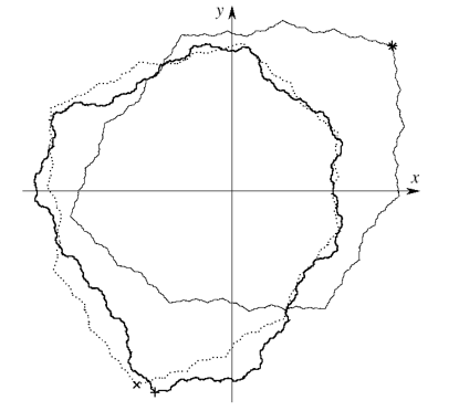
Figure 1: Critical points $c$ and Siegel disks of the map (3) for $\sigma=\langle 1^{\infty}\rangle=\frac{1}{2}(\sqrt{5}-1)$ ($*$ and a thin line), $\sigma=\langle 5^{\infty}\rangle=\frac{1}{2}(\sqrt{29}-5)$ ($+$ and a thick line), and $\sigma=\langle 51^{\infty}\rangle=\frac{1}{38}(9-\sqrt{5})$ ($\times$ and a dotted line).

In all cases the only critical point, $c=-\frac{1}{2}{\mathrm{e}}^{2\pi i\sigma}$, is simple: $f^{\prime}(c)=0$, $f^{\prime\prime}(c)=2\neq 0$.

In this paper we study maps of the form

$$f_{m,\sigma,\beta}(z)=\frac{1}{\beta}{\mathrm{e}}^{2\pi i\sigma}\left[g_{m+1}(z)-(1-\beta)g_{m}(z)\right]\ ,$$ (4)

where $m\in{\mathbb{N}}$, $\beta$ is a complex parameter, and the function $g_{m}:{\mathbb{C}}\to{\mathbb{C}}$ is defined as

$$g_{m}(z)=\frac{1}{m+1}\left[1-(1-z)^{m+1}\right]\ .$$

Let $f$ be a map of the form (1), and $c$ be its critical point that belongs to the boundary of the Siegel disk of this map (we will only consider cases where $\partial{\mathcal{D}}$ contains one critical point). Let $d$ be the multiplicity of the critical point $c$, i.e., $f^{(k)}(c)=0$ for $k=1,2,\ldots,d$, and $f^{(d+1)}(c)\neq 0$. We will call $d$ the order of the critical point.

Noticing that, for the map (4),

$$f^{\prime}_{m,\sigma,\beta}(z)={\mathrm{e}}^{2\pi i\sigma}(1-z)^{m}\left(1-\frac{z}{\beta}\right)\ ,$$

we see that $f_{m,\sigma,\beta}(0)=0$, $f^{\prime}_{m,\sigma,\beta}(0)={\mathrm{e}}^{2\pi i\sigma}$, and, more importantly, if $\beta\neq 1$, the point $z=1$ is a zero of $f^{\prime}_{m,\sigma,\beta}$ of multiplicity $m$, while, for $\beta=1$, the point $z=1$ is a zero of $f^{\prime}_{m,\sigma,\beta}$ of multiplicity $m+1$. As long as the critical point $z=\beta$ is outside the closure of the Siegel disk, the scaling properties of the iterates on $\partial{\mathcal{D}}$ in the case of Diophantine $\sigma$ are determined by the order $d$ of the critical point $z=1$. Below by “critical point” we will mean the critical point that belongs to $\partial{\mathcal{D}}$. One of the goals of this paper is to study how the regularity and the scaling properties depend on the order of the critical point.

In Figure 2 we show about 16 million iterates

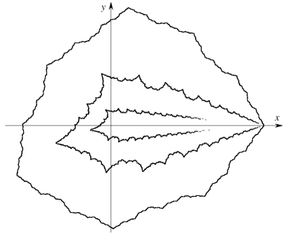
Figure 2: Siegel disks of the maps $f_{d,\langle 2^{\infty}\rangle,1+3i}$ (given by (4)) with critical point $c=1$ of order $d=1$ (outermost curve), $d=5$, and $d=20$ (innermost curve) – see text for details.

of the critical point $c=1$ of the maps $f_{d,\langle 2^{\infty}\rangle,1+3i}$ for order $d=1$, 5, and 20, of the critical point $c=1$ (the other critical point, $\beta=1+3i$, is not in the closure of the Siegel disks, so is irrelevant for the problem studied). Note that, especially for highly critical maps, the iterates approach the critical point very slowly because the modulus of the scaling exponent becomes close to 1 (see Table 2).

II.2 Parameterization of the boundary of a Siegel disk

In the cases considered here, the boundaries of Siegel disks cannot be written in polar coordinates as $r=R(\theta)$ (because some rays $\theta=\mathrm{const}$ intersect $\partial{\mathcal{D}}$ more than once). In this section we explain how to parameterize $\partial{\mathcal{D}}$, and define the functions whose regularity we study numerically.

Once we know that a critical point $c$ is in the boundary of the Siegel disk ${\mathcal{D}}$ (which in the cases we consider is guaranteed by the results of Graczyk and Świa̧tek (2003)), it is easy to obtain a parameterization of the boundary which semiconjugates the map $f$ to a rotation.

It is known from the mathematical theory that $h$ – which is univalent in the open disk $B(0,r_{\mathrm{S}})$ – can be extended to the boundary of $B(0,r_{\mathrm{S}})$ as a continuous function thanks to the Osgood-Taylor-Carathéodory Theorem (see, e.g., (Henrici, 1974, Section 16.3) or (Burckel, 1979, Section IX.4)).

A dynamically natural parameterization $\chi$ of $\partial{\mathcal{D}}$ is obtained by setting

$$\chi(t)=h\left(r_{\mathrm{S}}\,{\mathrm{e}}^{2\pi i(t+\theta)}\right)\ ,$$ (5)

where $\theta$ is a constant to be chosen later. From (2), it follows that

$$f\circ\chi(t)=\chi(t+\sigma)$$ (6)

with $\chi(0)=c$. Since we know that in our cases the critical point $c$ is in $\partial{\mathcal{D}}$, $|h^{-1}(c)|=r_{\mathrm{S}}$, and we can choose $\theta$ so that

$$\chi(0)=h(r_{\mathrm{S}}\,{\mathrm{e}}^{2\pi i\theta})=c\ .$$ (7)

In summary, the function $\chi:{\mathbb{T}}\to{\mathbb{C}}$ defined by (5) and (7) is a parameterization of $\partial{\mathcal{D}}$ such that the dynamics of the map $f$ on $\partial{\mathcal{D}}$ is a rotation by $\sigma$ on the circle ${\mathbb{T}}$, and $\chi(0)$ is the critical point.

Iterating $n$ times (6) for $t=0$, and using (7), we obtain

$$\chi(n\sigma)=f^{n}(c)\ .$$ (8)

Since the rotation number $\sigma$ of $f$ is irrational, the numbers $n\sigma$ (taken mod 1) are dense on the circle ${\mathbb{T}}$, and the iterates $f^{n}(c)$ of the critical point $c$ are dense on $\partial{\mathcal{D}}$ as well. Hence, using equation (8), we can compute a large number of values of $\chi$ by simply iterating $f$.

Our main object of interest are the real, $\Re\chi$, and imaginary, $\Im\chi$, parts of the function $\chi$. In Figure 3 we have shown the graphs of the real and imaginary parts of $\chi$ parameterizing the boundary of the Siegel disk of the map (3) for two different rotation numbers.

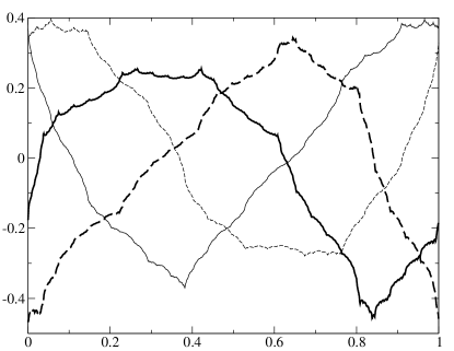
Figure 3: Graphs of the real (solid lines) and the imaginary (dashed lines) parts of the map $\chi$ corresponding to $\partial{\mathcal{D}}$ of the map (3) for $\sigma=\langle 1^{\infty}\rangle$ (thin lines) and $\sigma=\langle 5^{\infty}\rangle$ (thick lines) – cf. Figure 1.

II.3 Continued fraction expansions and rational approximations

In this section, we collect some of the notation on continued fraction expansions.

Let ${\mathsf{A}}=(a_{1},a_{2},\ldots,a_{p})$ be a finite sequence of $p$ natural numbers $a_{j}\in{\mathbb{N}}$; for brevity, we will usually omit the commas and write ${\mathsf{A}}=(a_{1}a_{2}\ldots a_{p})$. Let ${\mathsf{B}}=(b_{1}b_{2}\ldots b_{q})$ be another sequence of natural numbers $b_{j}\in{\mathbb{N}}$, $j=1,2,\ldots,q$, ${\mathsf{A}}{\mathsf{B}}:=(a_{1}a_{2}\ldots a_{p}b_{1}b_{2}\ldots b_{q})$ stand for the concatenation of ${\mathsf{A}}$ and ${\mathsf{B}}$, and ${\mathsf{A}}^{n}$ stand for ${\mathsf{A}}{\mathsf{A}}\cdots{\mathsf{A}}$ ($n$ times). Let $|{\mathsf{A}}|=p$ denote the length of ${\mathsf{A}}$.

For $a\in{\mathbb{N}}$ define the function ${\mathcal{F}}_{a}:(0,1)\to(0,1)$ by ${\mathcal{F}}_{a}(x):=\displaystyle{\frac{1}{a+x}}$. Similarly, for ${\mathsf{A}}=(a_{1}a_{2}\ldots a_{p})$, define the function ${\mathcal{F}}_{\mathsf{A}}:(0,1)\to(0,1)$ as the composition

$${\mathcal{F}}_{\mathsf{A}}(x):={\mathcal{F}}_{a_{1}}\circ{\mathcal{F}}_{a_{2}}\circ\cdots\circ{\mathcal{F}}_{a_{p}}(x)\ .$$

Let $\langle{\mathsf{B}}\rangle$ stand for the number whose continued fraction expansion (CFE) is given by the numbers in the sequence ${\mathsf{B}}$:

$$\langle{\mathsf{B}}\rangle=\langle b_{1}b_{2}\ldots b_{q}\rangle:=\displaystyle{\frac{1}{b_{1}+\displaystyle{\frac{1}{b_{2}+\displaystyle{\frac{1}{\ddots+\displaystyle{\frac{1}{b_{q}}}}}}}}}\ ;$$

the numbers $b_{j}$ are called the (partial) quotients of $\langle{\mathsf{B}}\rangle$. A number $\sigma=\langle a_{1}a_{2}\ldots\rangle$ is of bounded type if all numbers $a_{i}$ ($i\in{\mathbb{N}}$) are bounded above by some constant $M$.

We are especially interested in studying numbers with CFEs of the form

$$\langle{\mathsf{A}}{\mathsf{B}}^{\infty}\rangle:=\lim_{n\to\infty}\langle{\mathsf{A}}{\mathsf{B}}^{n}\rangle\ ,$$

which are called eventually periodic (or preperiodic). Since each number of this type is a root of a quadratic equation with integer coefficients (see (Hardy and Wright, 1990, Theorem 176)), such numbers are also called quadratic irrationals. We will call ${\mathsf{A}}$ the head and ${\mathsf{B}}^{\infty}$ the tail, ${\mathsf{B}}$ the period, and $|{\mathsf{B}}|$ the length of the period of the CFE.

If two quadratic irrationals have the same tail, they are said to be equivalent. One can prove that $\sigma$ and $\rho$ are equivalent if and only if $\sigma=(\iota\rho+\lambda)/(\mu\rho+\nu)$, where the integers $\iota$, $\lambda$, $\mu$ and $\nu$ satisfy $\iota\nu-\lambda\mu=\pm 1$ (Hardy and Wright, 1990, Theorem 175).

II.4 Scaling exponents

Let $f$ be a map of the form (1) with an eventually periodic rotation number $\sigma=\langle{\mathsf{A}}{\mathsf{B}}^{\infty}\rangle$ with length of its period $q=|{\mathsf{B}}|$, and let $c$ be the critical point of $f$ on $\partial{\mathcal{D}}$ (and there are no other critical points on $\partial{\mathcal{D}}$). Let

$$\frac{P_{m}}{Q_{m}}=\langle{\mathsf{A}}{\mathsf{B}}^{m}\rangle\ ,$$ (9)

where $P_{m}$ and $Q_{m}$ are natural numbers that have no common factors. Define the scaling exponent

$$\alpha:=\lim_{m\to\infty}\displaystyle{\frac{f^{Q_{m+1}}(c)-c}{f^{Q_{m}}(c)-c}}\ .$$ (10)

This exponent is a complex number that depends on the tail ${\mathsf{B}}$ of the CFE of $\sigma$ and on the order of the critical point $c$, but does not depend on the head ${\mathsf{A}}$ or on details about the map $f$.

If the length $|{\mathsf{B}}|$ of the tail ${\mathsf{B}}$ of the CFE of the rotation number of the map is more than 1, then ${\mathsf{B}}$ is determined only up to a cyclic permutation, and the argument of the complex number $\alpha$ is different for different choices. That is why we give our data only for $|\alpha|$.

III Hölder regularity and scaling properties of the boundaries of Siegel disks – numerical methods and results

III.1 Some results from harmonic analysis

Let ${\kappa}=n+{\kappa}^{\prime}$, where $n\in\{0,1,2,\ldots\}$, and ${\kappa}^{\prime}\in(0,1)$. We say that a function $\phi:{\mathbb{T}}\to{\mathbb{T}}$ has (global) Hölder regularity ${\kappa}$ and write $\phi\in C^{{\kappa}}({\mathbb{T}})$ if ${\kappa}=n+{\kappa}^{\prime}$ is the largest number for which $\phi^{(n)}$ exists and for some constant $C>0$ satisfies

$$\left|\phi^{(n)}(t)-\phi^{(n)}\left(s\right)\right|\leq C\,\left|t-s\right|^{{\kappa}^{\prime}}\qquad\forall\ t,s\in{\mathbb{T}}\ .$$

We call attention to the fact that we do not allow ${\kappa}$ to be an integer since otherwise the definition of Hölder so that the characterizations we discuss later must be modified. In our problem, ${\kappa}$ turns out to be non-integer, so that the characterizations we discuss apply.

In the mathematical literature, there are many characterizations of the Hölder regularity of functions. Some surveys that we have found useful are Stein (1970); Krantz (1983).

In the paper de la Llave and Petrov (2002), we developed implementations of several criteria for determining Hölder regularity numerically based on harmonic analysis, and assessed the reliability of these criteria. In this paper, we only use one of them, namely the method that we called the Continuous Littlewood-Paley (CLP) method which has been used in Carletti (2003); Apte et al. (2005); Fuchss et al. (2006); Olvera and Petrov (to appear, 2008). The CLP method is based on the following theorem Stein (1970); Krantz (1983):

Theorem III.1.

A function $\phi\in C^{{\kappa}}(\mathbb{T})$ if and only if for some $\eta>0$ there exists a constant $C>0$ such that for all $\tau>0$ and $\eta\geq 0$

$$\left\|\left(\frac{\partial}{\partial\tau}\right)^{\eta}\mathrm{e}^{-\tau\sqrt{-\Delta}}\,\phi\right\|_{L^{\infty}({\mathbb{T}})}\leq C\,\tau^{{\kappa}-\eta}\ ,$$ (11)

where $\Delta$ stands for the Laplacian: $\Delta\phi(t)=\phi^{\prime\prime}(t)$.

Note that one of the consequences of Theorem III.1 is that if the bounds (11) hold for some $\eta$, they hold for any other $\eta$. Even if from the mathematical point of view, all values of $\eta$ would give the same result, it is convenient from the numerical point of view to use several to assess the reliability of the method.

III.2 Algorithms used

The algorithm we use is based on the fact that $\left(\frac{\partial}{\partial\tau}\right)^{\eta}\mathrm{e}^{-\tau\sqrt{-\Delta}}$ is a diagonal operator when acting on a Fourier representation of the function: if

$$\phi(t)=\sum_{k\in{\mathbb{N}}}\widehat{\phi}_{k}\,{\mathrm{e}}^{-2\pi ikt}\ ,$$

then

$$\left(\frac{\partial}{\partial\tau}\right)^{\eta}\mathrm{e}^{-\tau\sqrt{-\Delta}}\phi(t)=\sum_{k\in{\mathbb{N}}}(-2\pi|k|)^{\eta}\,{\mathrm{e}}^{-2\pi\tau|k|}\,\widehat{\phi}_{k}\,{\mathrm{e}}^{-2\pi ikt}\ .$$

The Fourier transform of the function $\phi$ can be computed efficiently if we are given the values of $\phi(t)$ on a dyadic grid, i.e., at the points $t_{m}=2^{-M}m$, where $M$ is some natural number and $m=0,1,\ldots,2^{M}-1$. Unfortunately, the computation indicated in (8) gives the values of the function $\chi=\Re\chi+i\,\Im\chi$ on the set $\{n\sigma\}_{n=0}^{N}$ of translations by the irrational number $\sigma$. Therefore, we need to perform some interpolation to find the approximate values of $\chi$ on the dyadic grid, after which we Fast Fourier Transform (FFT) can be computed efficiently.

Hence, the algorithm to assess the regularity is the following.

1. Locate the critical point $c$ (such that $f^{\prime}(c)=0$).

2. Use equation (8) to obtain the values of the function $\chi$ at the points $\{n\sigma\}_{n=0}^{N}$ for some large $N$.

3. Interpolate $\Re\chi$ and $\Im\chi$ to find their approximate values on the dyadic grid $\{2^{-M}m\}_{m=0}^{2^{M}-1}$.

4. For a fixed value of $\eta$, compute the value of the left hand side of (11) for several values of $\tau$ by using FFT (for $\phi=\Re\chi$ and separately for $\phi=\Im\chi$); do this for several values of $\eta$.

5. Fit the decay predicted by (11) to find the regularity ${\kappa}$.

Let us estimate the cost in time and storage of the algorithm above keeping $2^{M}$ values of the function. Of course, locating the critical point $c$ is trivial. Iteration and interpolation require $O(2^{M})$ operations. Then, each of the calculations of (11) requires two FFT, which is $O(2^{M}\ln(2^{M}))=O(M\,2^{M})$. In the computers we used (with about $1\,\mathrm{GB}$ of memory) the limiting factor was the storage, but keeping several million iterates of $f$ and computing $2^{23}\approx 8\times 10^{6}$ Fourier coefficients of $\Re\chi$ and $\Im\chi$ was quite feasible. (Note that a double precision array of $2^{23}$ double complex numbers takes $2^{27}$ bytes $=128\,{\rm MB}$ and one needs to have several copies.)

The iterates $f^{n}(c)$ were computed by using extended precision with GMP – an arbitrary-precision extension of $C$ language GMP (2008). This extra precision is very useful to avoid that the orbit scales. Note that the critical points are at the boundary of the domains of stability, so that they are moderately unstable.

The extended precision is vitally important in computing the scaling exponents $\alpha$. To obtain each value in Table 2, we computed several billion iterates of the critical point of the map. To reduce the numerical error, we used several hundred digits of precision.

III.3 Visual explorations

In Figures 4 and 5

Figure 4: Plot of $\log_{10}|\,(\widehat{\Re\chi})_{k}|$ vs. $\log_{10}|k|$ for the map (3) with $\sigma=\langle 1^{\infty}\rangle$ – see text for details.

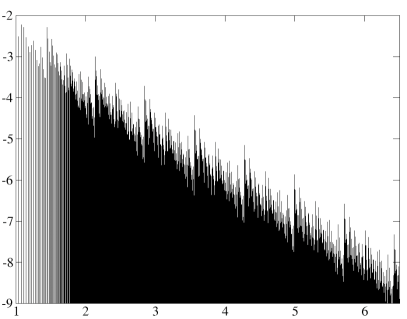
Figure 5: Plot of $\log_{10}|\,(\widehat{\Re\chi})_{k}|$ vs. $\log_{10}|k|$ for the map (3) with $\sigma=\langle 5^{\infty}\rangle$ – see text for details.

we have plotted (with impulses) the modulus of the Fourier coefficients $(\widehat{\Re\chi})_{k}$ versus $|k|$ on a log-log scale (for several million values of $k$) for the boundary of the Siegel disk corresponding to the map (3) for rotation numbers $\sigma$ equal to $\langle 1^{\infty}\rangle$ and $\langle 5^{\infty}\rangle$, and order of the critical point $d=1$ (the same cases as the ones in Figures 1 and 3). The self-similar structure of the boundary of the Siegel disk is especially clearly visible in the “straightened-out” graph of the spectrum – in Figure 6 we plotted $\log_{10}|k\,(\widehat{\Re\chi})_{k}|$ vs. $\log_{10}|k|$ for the same spectra as in Figures 4 and 5.

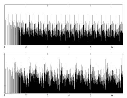
Figure 6: Plot of $\log_{10}|k\,(\widehat{\Re\chi})_{k}|$ vs. $\log_{10}|k|$ for the map (3) with $\sigma=\langle 1^{\infty}\rangle$ (top), $\sigma=\langle 5^{\infty}\rangle$ (bottom) – see text for details.

The width of each of the periodically repeating “windows” in the figure (i.e., the distance between two adjacent high peaks) is approximately equal to $|\log_{10}\sigma|$, where $\sigma$ is the corresponding rotation number. The periodicity in the Fourier series has been related to some renormalization group analysis in phase space Shraiman (1984).

To illustrate the effect of the order of criticality on the Fourier spectrum of $\Re\chi$, we showed in Figure 7 the “straightened-out” graphs of the spectra, $\log_{10}|k\,(\widehat{\Re\chi})_{k}|$ versus $\log_{10}|k|$, of the function $\Re\chi$ corresponding to the maps $f_{d,\langle 2^{\infty}\rangle,1+3i}$ for orders $d=1,5,20$ (the Siegel disks of these maps were shown in Figure 2). For all plots in this figure we used the same scale in vertical direction. An interesting observation – for which we have no conceptual explanation at the moment – is that the variability of the magnitudes of the Fourier coefficients decreases as the order of the critical point increases.

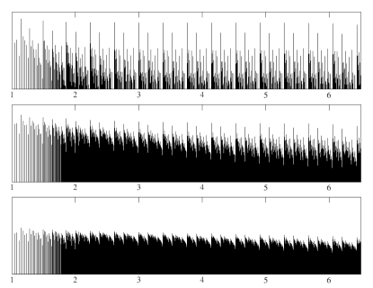
Figure 7: Plot of $\log_{10}|k\,(\widehat{\Re\chi})_{k}|$ vs. $\log_{10}|k|$ for the maps $f_{d,\langle 2^{\infty}\rangle,1+3i}$ with $d=1,5,20$.

Figures 8 and 9 illustrate the CLP method (Theorem III.1) in practice.

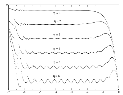
Figure 8: Top: Plot of $\log_{10}N_{\eta}(\tau)$ vs. $\log_{10}\tau$ for the map (3) with $\sigma=\langle 1^{\infty}\rangle$. Bottom: Plot of the first differences between the vertical coordinates of adjacent points in the top figure.

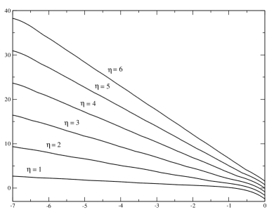
Figure 9: Top: Plot of $\log_{10}N_{\eta}(\tau)$ vs. $\log_{10}\tau$ for the map (3) with $\sigma=\langle 5^{\infty}\rangle$. Bottom: Plot of the first differences between the vertical coordinates of adjacent points in the top figure.

In the top part of each figure we have plotted on a log-log scale the norms in the left-hand side of (11),

$$N_{\eta}(\tau):=\left\|\left(\frac{\partial}{\partial\tau}\right)^{\eta}\,{\mathrm{e}}^{-\tau\sqrt{-\Delta}}\,\Re\chi\right\|_{L^{\infty}({\mathbb{T}})}\ ,$$ (12)

as functions of $\tau$, for $\eta=1,2,\ldots,6$ for the map (3) with for rotation numbers $\langle 1^{\infty}\rangle$ and $\langle 5^{\infty}\rangle$, respectively. For each value of $\eta$, the “line” consists of 400 points corresponding to 400 different values of $\tau$ for which we have computed the corresponding norm.

The bottom parts of Figures 8 and 9 show the behavior of the first differences between the vertical coordinates of adjacent points from the top parts of the figures. Clearly, the points in the top parts do not lie on exact straight lines but have small periodic (as functions of $\log\tau$) displacements. To make this more clear in the bottom part of Figure 9, we have plotted the points for $\eta=6$ with larger circles, and have connected them with lines.

We would like to point out that the bound (11) is only an upper bound. However, the discrete scaling invariance of the Siegel disk at small scales – manifested also by the existence of the “periodic windows” in Figure 6 – implies that the leading behavior of $\log_{10}N_{\eta}(\tau)$ as a function of $\log_{10}\tau$ is indeed linear, and that (11) is close to being saturated.

The discrete scaling invariance at small scales allows for $\log_{10}N_{\eta}(\tau)$ as a function of $\log_{10}\tau$ to have small periodic corrections superimposed on the leading linear behavior. Our calculations are precise enough that these corrections to the leading behavior are clearly visible. The bottom parts of Figures 8 and 9 show exactly these corrections.

The form of these small periodic corrections depends in a complicated way on the the behavior of the Fourier coefficients in the “periodic windows” in the Fourier spectrum. The presence of this periodic corrections is a good indicator of the ranges of $t$ which are large enough that the asymptotic behaviour has started to take hold, but small enough so that they are not dominated by the round-off and truncation error. In our previous works de la Llave and Petrov (2002); Apte et al. (2005), we have also found periodic corrections to the scaling in other conjugacies related to the regularity of conjugacies of other critical objects.

III.4 Numerical values of the Hölder regularity

In Table 1 we give the computed values

Table 1: Global Hölder regularity ${\kappa}$ for maps with rotation numbers $\sigma=\langle k^{\infty}\rangle$ ($k=1,2,3,4,5$) and critical point of order $d$.

$d$	$\langle 1^{\infty}\rangle$	$\langle 2^{\infty}\rangle$	$\langle 3^{\infty}\rangle$	$\langle 4^{\infty}\rangle$	$\langle 5^{\infty}\rangle$
1	0.621	0.617	0.607	0.596	0.578
2	0.432	0.427	0.417	0.404	0.388
3	0.328	0.324	0.313	0.300	0.291
4	0.263	0.260	0.252	0.244	0.232
5	0.220	0.217	0.210	0.203	0.193
6	0.189	0.186	0.180	0.174	0.163
10	0.121	0.120	0.115	0.111	0.105
15	0.084	0.082	0.079	0.077	0.074
20	0.064	0.063	0.061	0.058	0.055

of the global Hölder regularities of the real and imaginary parts of the dynamically natural parameterizations $\chi$ (5), (7) of the boundaries of the Siegel disks. We studied maps of the form (4), with different values of $\beta$, and with different orders $d$ of the critical point in $\partial{\mathcal{D}}$; some runs with the map (3) (for which the critical point is simple) were also performed.

To obtain each value in the table, we performed the procedure outlined in Section III.2 for at least two maps of the form (4). For each map we plotted the points from the CLP analysis for $\eta=1,2,\ldots,6$ as in the top parts of Figures 8 and 9, looked at the differences between the vertical coordinates of adjacent points (i.e., at graphs like in the bottom parts of Figures 8 and 9), and selected a range of values of $\log_{10}\tau$ for which the differences oscillate regularly. For this range of $\log_{10}\tau$, we found the rate of decay of the norms $N_{\eta}(\tau)$ (12) by measuring the slopes, ${\kappa}-\eta$, from which we computed the regularity ${\kappa}$.

The accuracy of these values is difficult to estimate, but a conservative estimate on the relative error of the data in Table 1 is about 3%.

We have also computed the regularity ${\kappa}$ and the scaling exponent $\alpha$ of several maps with rotation numbers with the same tails of the continued fraction expansion but with different heads.

Within the accuracy of our computations, the results did not depend on the head, which is consistent with the predictions of the renormalization group picture.

III.5 Importance of the phases of Fourier coefficients

In Figure 6 we saw that the modulus of the Fourier coefficients of $\Re\chi$ and $\Im\chi$ decreases very approximately as

$$\left|(\widehat{\Re\chi})_{k}\right|\leq\frac{C}{|k|}\ ,\qquad\left|(\widehat{\Im\chi})_{k}\right|\leq\frac{C}{|k|}\ .$$ (13)

and that these bounds come close to be saturated infinitely often. This seems to be true independent of what the rotation number is.

This rate of decay of the Fourier coefficients would be implied by $\Re\chi$ and $\Im\chi$ being $C^{1}$, but from (13) we cannot conclude that $\Re\chi$ and $\Im\chi$ are even continuous (note, for example, that the function $f(x)=\sum_{k=1}^{\infty}\frac{1}{k}\cos kx$ is discontinuous at $x=0$). It is well-known from harmonic analysis that the phases of the Fourier coefficients play a very important role, and changing the phases of Fourier coefficients changes the regularity of the functions (see, e.g., Zygmund (2002))

$$\sum_{k=2}^{\infty}\,\frac{1}{k^{1/4}}\,\,e^{2\pi ikx}\sim\frac{1}{|x|^{3/4}}\quad\mbox{as}\ |x|\to 0\ ,$$

while

$$\sum_{k=2}^{\infty}\,\frac{e^{i\sqrt{k}}}{k^{1/4}}\,\,e^{2\pi kx}\sim\frac{1}{|x|^{2}}\quad\mbox{as}\ |x|\to 0\ .$$

In Figure 10 we depict the phases of the Fourier coefficients of $\Re\chi$ for the map $f_{0,\langle 1^{\infty}\rangle,1}$ whose only critical point, $c=1$, is simple (i.e., of order $d=1$).

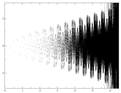
Figure 10: Plot of the phases of the Fourier coefficients (vs. $\log_{10}|k|$) of $\Re\chi$ for the map $f_{0,\langle 1^{\infty}\rangle,1}$.

We see that, for small $k$, the phases have a repeated pattern. If we consider $k\in I_{j}:=[\sigma^{-j},\sigma^{-j-1}]$ (where $\sigma=\langle 1^{\infty}\rangle$ is the golden mean), we see that the phase restricted to $I_{j}$ has a pattern very similar to $I_{j+1}$, except that the latter is reversed and amplified. Of course, since the phase only takes values between $-\pi$ and $\pi$, the amplification of the patterns can only be carried out a finite number of times until the absolute values of the phases reach $\pi$, after which they will start “wrapping around” the interval $[-\pi,\pi]$. Unfortunately, to see this effect numerically, we would need hundreds of millions of Fourier coefficients, which at the moment is out of reach.

Given the above observation, it is natural to study the distribution of the phases of the Fourier coefficients in an interval of self-similarity. In Figure 11 we present the histogram

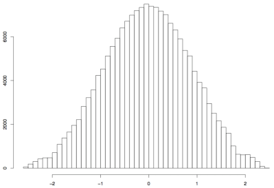
Figure 11: Histogram of some of the phases shown in Figure 10 (from $I_{24}\cup I_{25}$).

of the phases in the interval $k\in I_{24}\cup I_{25}=[\sigma^{-24},\sigma^{-26}]$ (i.e., of about 170,000 phases). We note that the histogram is very similar to a Gaussian. This visual impression is confirmed by using the Kolmogorov-Smirnov test, shown in Figure 12.

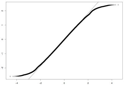
Figure 12: Kolmogorov-Smirnov test for normality of the phases in $I_{24}\cup I_{25}$.

Recall that the Kolmogorov-Smirnov test consists in plotting the empirical distribution versus the theoretical one (for details see, e.g., (Sheskin, 2007, Chapter 7)). If indeed the empirical distribution was a sample of the theoretical distribution, we would get a set of points close the diagonal. The Kolmogorov-Smirnov test is available in many statistical packages (we used the package R, in which the command qqnorm gives a KS-test and the command qqline displays the result of a fitted Gaussian). The Kolmogorov-Smirnov test reveals that, as expected (since the variable is an angle), the distribution of the phases has discrepancies with a Gaussian near the edges, $-\pi$ and $\pi$. Nevertheless, there is a remarkably good fit away from these edges. For the intervals we chose, most of the data points are indeed out of the edges.

III.6 Data on the scaling exponents

In Table 2

Table 2: Values of $|\alpha|$ for maps of the form $f_{d,\sigma,\beta}$ (4) with different rotation numbers $\sigma$ and orders $d$ of the critical point.

$d$	$\langle 1^{\infty}\rangle$	$\langle 2^{\infty}\rangle$	$\langle 3^{\infty}\rangle$	$\langle 4^{\infty}\rangle$	$\langle 5^{\infty}\rangle$
1	0.74193223170	0.5811130545	0.484541021	0.424632459	0.385769294
2	0.81215810740	0.686013947	0.607281233	0.55822367	0.5268809
3	0.853450202	0.7508249	0.6852424	0.6441419	0.6179964
4	0.88014575	0.793968	0.738015	0.7027580	0.680345
5	0.8987131	0.824557	0.775859	0.7450319	0.725425
6	0.912340	0.847314	0.804246	0.7768796	0.759458
10	0.943087	0.89962	0.87026	0.851416	0.839375
15	0.960463	0.92977	0.90881	0.895266	0.88658
20	0.969717	0.94601	0.92971	0.919149	0.91236
40	0.984450	0.97211	0.96356	0.9579	0.9544
60	0.989504	0.981138	0.975314	0.97151	0.96906
80	0.9920788	0.98575	0.981334	0.97845	0.97658
100	0.993638	0.98854	0.98499	0.98267	0.98116
200	0.996793	0.99422	0.99242	0.991241	0.99048
300	0.997857	0.99613	0.99493	0.994140	0.99363

we give the values of the modulus of the scaling exponent $\alpha$ for maps of the form (3) with orders $d=1,\ldots,6,10,15,20,40,60,80,100$ of the critical point and rotation numbers $\sigma=\langle k^{\infty}\rangle$ with $k=1,\ldots,5$. We believe that the numerical error in these values does not exceed 2 in the last digit.

In Osbaldestin (1992), the author computed the scaling exponents for maps with rotation number $\langle 1^{\infty}\rangle$ and critical point of different orders $d$, and suggested that the behavior of $\alpha$ for large $d$ is

$$|\alpha_{\langle 1^{\infty}\rangle,d}|\sim 1-\frac{A_{\langle 1^{\infty}\rangle}}{d}\qquad\mbox{ as }\ d\to\infty\ .$$ (14)

We studied the same problem for other rotation numbers and, taking advantage of the extended precision, we carried out the computation for rather high degrees of criticality ($\approx 300$), see Table 2. In Figure 13 we plotted $1/(1-|\alpha|)$ versus $d$ for five rotation numbers. Our data that for high values of $d$ the modulus of $\alpha$ tends to 1 for any rotation number. The values of the constants $A_{\sigma}$ in (14) for rotation numbers $\langle k^{\infty}\rangle$ with $k=1,2,3,4,5$ are approximately $0.646$, $1.168$, $1.531$, $1.960$, $1.925$, respectively (the linear regression was based on the values for $d=40,\ldots,300$).

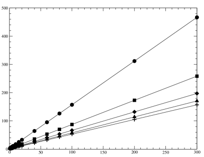
Figure 13: Plot of $1/(1-|\alpha|)$ vs. $d$ for rotation numbers $\langle 1^{\infty}\rangle$ (circles), $\langle 2^{\infty}\rangle$ (squares), $\langle 3^{\infty}\rangle$ (diamonds), $\langle 4^{\infty}\rangle$ (triangles), $\langle 5^{\infty}\rangle$ (pluses).

IV Calculation of the Siegel radius and the area of the Siegel disk

As a byproduct of our calculations we can obtain rather precise values of two quantities of mathematical interest: the area of the Siegel disk and the Siegel radius.

IV.1 Calculation of Siegel radius

We note that the parameterization, $\chi$, of the boundary $\partial{\mathcal{D}}$ is related to the conjugacy $h$ (2) by (5). Then, the Fourier coefficients of $\chi$ satisfy $|\hat{\chi}_{-k}|=|h_{k}|\,r_{\mathrm{S}}^{k}$ for $k\in{\mathbb{N}}$, where $h_{k}$ are the Taylor coefficients of $h$ (recall that $h_{0}=0$ and $h_{1}=1$). As shown in Siegel and Moser (1995); de la Llave (2001), one can get the all the coefficients $h_{k}$ by equating terms of like powers in (2), and this gives infinitely many different ways to compute $r_{\mathrm{S}}$. In particular, since $h_{1}=1$, we have $r_{\mathrm{S}}=|\hat{\chi}_{-1}|$. Since we also have $h_{2}=f_{2}/[a(a-1)]$ and $|a|=1$, we obtain $r_{\mathrm{S}}^{2}=|a-1||\hat{\chi}_{-2}|/|f_{2}|$ (where $f_{1}=a$, $f_{2}$, $\ldots$ are the Taylor coefficients of the function $f$). Similar formulas for higher order terms are also available.

IV.2 Calculation of the area of the Siegel disk

Since $h(r_{\mathrm{S}}z)$ is a univalent mapping from the unit disk to the Siegel disk, we can use the area formula Rudin (1987)

$${\rm Area}=\pi\sum_{k=1}^{\infty}k|h_{k}|^{2}=\pi\sum_{k=1}^{\infty}kr_{\mathrm{S}}^{-2k}|\hat{\chi}_{-k}|^{2}\ .$$ (15)

For polynomials, the Siegel disk is bounded so that the sum in (15) is finite. This is compatible with the observation (13), but it shows that the bound cannot be saturated very often.

In Table 3

Table 3: Areas of the Siegel disks for maps of the form $f_{d,\langle k^{\infty}\rangle,1+3i}$ (see (4)) with different rotation numbers $\sigma$ and orders $d$ of the critical point.

$d$	$\langle 1^{\infty}\rangle$	$\langle 2^{\infty}\rangle$	$\langle 3^{\infty}\rangle$	$\langle 4^{\infty}\rangle$	$\langle 5^{\infty}\rangle$
1	1.3603361	1.3586530	1.3611085	1.3652030	1.3693337
2	0.895659	0.893442	0.893605	0.89408	0.89367
3	0.65986	0.65766	0.65664	0.6553	0.65308
4	0.5190	0.5170	0.51550	0.5133	0.5104
5	0.4262	0.4244	0.4226	0.4200	0.4170
6	0.3607	0.3591	0.3573	0.354	0.3515
10	0.2214	0.2203	0.2187	0.2163	0.2137
15	0.148	0.147	0.146	0.144	0.1421
20	0.111	0.110	0.109	0.107	0.106

we give the values of the areas of the Siegel disks of the map $f_{d,\sigma,\beta}$ (4) (we believe that the error does not exceed 2 in the last digit). Since the series (15) converges slowly, we computed the partial sums of the first $Q_{n}$ terms in (15), where $Q_{n}$ are the denominators of the best rational approximants, $P_{m}/Q_{m}=\langle k^{m}\rangle$, to the rotation number $\sigma=\langle k^{\infty}\rangle$ (cf. (9)), and then performed Aitken extrapolation on these values. Because of the repeating “periodic windows” in the Fourier spectra (shown in Figures 4, 5, 6, 7), these partial sums tend to the area of the Siegel disk geometrically, and Aitken extrapolation gives good results. In our computations we used $2^{23}\approx 8\times 10^{6}$ Fourier coefficients of $\chi$.

Clearly, the area of a Siegel disk depends on the particular choice of the map $f$, i.e., is non-universal. Perhaps the only universal characteristic that can be extracted is the rate of convergence in the Aitken extrapolation, but we have not studied this problem in detail.

V An upper bound of the regularity of the conjugacy

As pointed out in (de la Llave and Petrov, 2002, Section 8.2), one can find upper bounds for the regularity in terms of the scaling exponents.

Recall that $\chi:{\mathbb{T}}\to\partial{\mathcal{D}}$ conjugates (the restriction to $\partial{\mathcal{D}}$ of) the map $f:\partial{\mathcal{D}}\to\partial{\mathcal{D}}$ to the rigid rotation $r_{\sigma}:{\mathbb{T}}\to{\mathbb{T}}:t\mapsto t+\sigma$ (where $\sigma$ is the rotation number of $f$), namely, $\chi\circ r_{\sigma}=f\circ\chi$. Let us consider only rotation numbers of the form $\sigma=\langle k^{\infty}\rangle$, and let the natural numbers $Q_{m}$ and the scaling exponent $\alpha$ be defined by (9) and (10). Then closest returns of the iterates of $0\in{\mathbb{T}}$ of $r_{\sigma}$ and the iterates of $c\in\partial{\mathcal{D}}$ to the starting points $0$ and $c$, respectively, are governed by the scaling relations

$$r_{\sigma}^{Q_{m}}(0) = C_{1}\sigma^{m}+o(\sigma^{m})\ ,$$

$$|f^{Q_{m}}(c)-c| = C_{2}|\alpha|^{m}+o(|\alpha|^{m})\ .$$

So that we obtain that $h(C_{1}\sigma^{m})\approx C_{2}|\alpha|^{m}$.

This is impossible if $h$ is $C^{\kappa}$ with

$${\kappa}>{\kappa}_{\mathrm{max}}\equiv\log|\alpha|/\log\sigma$$ (16)

and the right-hand side of (16) is not an integer.

In Table 4,

Table 4: Upper bounds on the Hölder regularity ${\kappa}_{\mathrm{max}}$ (16) for maps of the form $f_{d,\sigma,\beta}$ (4) with rotation numbers $\sigma=\langle k^{\infty}\rangle$ ($k=1,2,3,4,5$) and critical point of order $d$.

$d$	$\langle 1^{\infty}\rangle$	$\langle 2^{\infty}\rangle$	$\langle 3^{\infty}\rangle$	$\langle 4^{\infty}\rangle$	$\langle 5^{\infty}\rangle$
1	0.6203	0.6159	0.6064	0.5933	0.5783
2	0.4324	0.4276	0.4175	0.4039	0.3890
3	0.3293	0.3252	0.3164	0.3047	0.2922
4	0.2653	0.2618	0.2543	0.2443	0.2338
5	0.2219	0.2189	0.2124	0.2039	0.1949
6	0.1906	0.1880	0.1823	0.1749	0.1670
10	0.1218	0.1200	0.1163	0.1114	0.1063
15	0.0838	0.0826	0.0800	0.0766	0.0731
20	0.0639	0.0630	0.0610	0.0584	0.0557

we give the values of the upper bound to the regularity ${\kappa}_{\mathrm{max}}$ (16) for maps with rotation numbers and order of the critical point. To compute these values, we used the values for $|\alpha|$ from Table 2 (and the exact values for the rotation numbers). We have kept only four digits of accuracy, although the error of these numbers is smaller (their relative error is the same as the relative error of the values of $|\alpha|$).

Clearly, within the numerical error, the values of the regularities from Table 1 (obtained from applying the CLP method) are equal to the upper bounds on the regularity from Table 4 (obtained from the scaling exponents).

This is in contrast with the results in de la Llave and Petrov (2002), where similar bounds based on scaling were found to be saturated by some conjugacies but not by the inverse conjugacy.

For maps with highly critical points, if (16) holds, then the asymptotic behavior of $|\alpha|$ (14) implies that the asymptotic behavior of the limit on the regularity becomes

$${\kappa}_{\mathrm{max},\sigma}\sim\frac{\log\left|1-\frac{A_{\sigma}}{d}\right|}{\log\sigma}\approx\frac{A_{\sigma}}{|\log|\sigma||}\,\frac{1}{d}\qquad\mbox{ as }\ d\to\infty\ .$$ (17)

VI Conclusions

We have considered Siegel disks of polynomials with some quadratic fields and with different degrees of critical points.

We have made extended precision calculations of scaling exponents and a parameterization of the boundary. This allows us to compute the regularity of the boundary using methods of harmonic analysis.

The regularity of the boundary seems to be universal, depend only on the tail of the continued fraction expansion and saturate some easy bounds in terms of the continued fraction expansion.

We have identified several regularities of the Fourier series of the conjugacy. Namely, it seems that, irrespective of the rotation number, we have $0<\limsup|k\hat{\chi}_{k}|<\infty$. There seems to be a regular distribution of the phases of the Fourier coefficients which follows a Gaussian law.

We have also extended the results of Osbaldestin (1992) on the dependence of scaling exponents on the degree of the critical point to higher degrees and to other rotation numbers.